Prototype Downscaling Algorithm for MODIS Satellite 1 km Daytime Active Fire Detections


1
ASRC Federal Data Solutions contractor to United States Geological Survey (USGS) Earth Resources Observation and Science (EROS) Center, Sioux Falls, SD 57198, USA
2
USGS EROS Center, Sioux Falls, SD 57198, USA
*
Author to whom correspondence should be addressed.
Fire 2019, 2(2), 29; https://0-doi-org.brum.beds.ac.uk/10.3390/fire2020029
Submission received: 18 April 2019
/
Revised: 19 May 2019
/
Accepted: 21 May 2019
/
Published: 23 May 2019
Abstract
:This work presents development of an algorithm to reduce the spatial uncertainty of active fire locations within the 1 km MODerate resolution Imaging Spectroradiometer (MODIS Aqua and Terra) daytime detection footprint. The algorithm is developed using the finer 500 m reflective bands by leveraging on the increase in 2.13 μm shortwave infrared reflectance due to the burning components as compared to the non-burning neighborhood components. Active fire presence probability class for each of the 500 m pixels within the 1 km footprint is assigned by locally adaptive contextual tests against its surrounding neighborhood pixels. Accuracy is assessed using gas flares and wildfires in conjunction with available high-resolution imagery. Proof of concept results using MODIS observations over two sites show that under clear sky conditions, over 84% of the 500 m locations that had active fires were correctly assigned to high to medium probabilities, and correspondingly low to poor probabilities were assigned to locations with no visible flaming fronts. Factors limiting the algorithm performance include fire size/temperature distributions, cloud and smoke obscuration, sensor point spread functions, and geolocation errors. Despite these limitations, the resulting finer spatial scale of active fire detections will not only help first responders and managers to locate actively burning fire fronts more precisely but will also be useful for the fire science community.
1. Introduction
Vegetation fires are routinely monitored from space using satellite data that detect the location of burned and actively burning locations at the time of over pass. Heritage active fire detection methodologies have been developed for different sensors using algorithms that take advantage of the elevated radiance of fire at longer middle infrared (MIR) wavelengths [1,2,3,4,5]. Satellite active fire detections have found applications in diverse fields including fire characterization studies [6,7,8,9,10,11], studies of human activity [12,13], examination of the ecological responses to fire [14,15], studies of active volcanism [16,17], estimation of pyrogenic emissions of greenhouse gases and aerosols [18,19] for wildfire fire monitoring, control, and natural resource management [20,21,22], and have also been used in burned area mapping algorithms [23,24,25,26].
Currently, satellite sensors with operational active fire sensing capabilities (Advanced Very High-Resolution Radiometer (AVHRR), MODerate resolution Imaging Spectroradiometer (MODIS), Sentinel 3, Visible Infrared Imaging Radiometer Suite (VIIRS), Geostationary Operational Environmental Satellite system (GOES), etc.) use geostationary and polar orbiting platforms and their spatial resolutions range from 375 m to over a few kilometers with temporal frequency ranging from every 15 min to about twice daily. However, sensors with high spatial resolution have low temporal resolution and conversely sensors with low temporal resolution have higher spatial resolution. It is well established that the ~1 km spatial resolution of currently available active fire products is too coarse to identify the landcover that is burning [27,28,29,30]. Fire is spatially and temporally ephemeral, thereby necessitating finer spatial and temporal resolution observations for monitoring. The recently available twice daily VIIRS 750 and 375 m active fire product [31,32] is a step in the right direction, and data since 20 January 2012 to current are available. Among the currently operational satellites with fire detection capabilities, the MODIS Aqua and Terra satellites [2] and Sentinel 3 A and B [33,34] have finer spatial resolution in the reflective visible-shortwave infrared (VIS-SWIR) bands that can be readily used to downscale the nominal 1 km active fire detections for observations going back to 1999.
In this paper, we present a straightforward approach with proof of concept results, and accuracy assessments to downscale the MODIS 1 km active fire detections to estimate the active fire location probabilities within the 500 m subpixels. The downscaling algorithm is based on established satellite-based active fire detection capabilities using VIS-SWIR reflectance [10,17,35,36,37,38]. These algorithms leverage on the increased radiance/reflectance in the 2 μm (SWIR) bands relative to the shorter (0.8 μm near-infrared (NIR)) wavelengths and elevated SWIR radiance/reflectance, to identify pixels that have actively burning components.
The downscaling algorithm adapts established work [10,17,35,36,37,38] to assign the probability of active fire presence to those 500 m subpixels within the 1 km active fire detection footprint. A downscaled 500 m active fire product from 1 km can potentially reduce the location and area uncertainty by one half and one quarter, respectively. Algorithm accuracy assessments are inferred by using concurrent Advanced Spaceborne Thermal Emission and Reflection Radiometer (ASTER) and available Google Earth™ imagery over two sites. Higher spatial resolution of active fire detections will not only help first responders and managers to more precisely locate actively burning fire fronts but will also be useful to the fire science community engaged in studies that consider the spatial patterns of fire and fire spread rates [9,20,39,40,41].
2. Data
2.1. MODIS Sensor
The MODIS sensor is onboard two polar-orbiting satellites (Terra: 10.30 a.m. Equatorial overpass time and Aqua: 1.30 p.m. Equatorial overpass time) that provide up to two daytime and two nighttime over passes at the equator [2]. MODIS land surface products are produced in a sinusoidal tile grid system covering the global land area in 460 tiles with each tile covering 10 degrees by 10 degrees at the equator. The MODIS sensor is a whiskbroom sensor and hence its observation footprint increases as a function of the scan angle [42,43]. Observations resampled to a uniform gridded product using nearest neighbor resampling is available as the Level 3 gridded product [43].
MODIS is a multispectral sensor with 36 bands spanning 0.4 μm to 14 μm. The nominal nadir spatial resolutions range from 250 m for the 0.85 μm (NIR) and 0.64 μm (red) bands to 500 m for the 0.46 μm, 0.55 μm, 1.24 μm, 1.64 μm and 2.13 μm reflective bands, and 1 km for midinfrared and thermal bands [44]. In this work, the Collection 6 [45] Level 3 MODIS sinusoidal equal area projected and gridded to 1 km MODIS Terra-based MOD14A1 and the MODIS Aqua-based MYD14A1 data products [46] available from the National Aeronautical and Space Administration (NASA) Land Processes Distributed Active Archive Center LPDAAC [47] are used. Specifically, the 0.85 μm (NIR) and 2.13 μm (SWIR) reflective bands are used in this work. The MOD/MYD active fire product identifies 1 km pixels with active fires by their increased radiances in the 4 μm band relative to non-burning pixels using locally adaptive contextual tests [2,45]. Each 1 km MODIS pixel in the active fire product is labeled as fire if a fire is detected, otherwise the pixel is assigned a value for land, cloud, water, or unknown/no data. The MODIS active fire product has commission and omission errors that have been well characterized. Commission errors are typically due to increased thermal contrast of hotter bare earth adjacent to cooler forests [38] and also due to overlapping sensor point spread functions [42,48]. Omissions are largely due to insufficient size and temperature of active fires encompassed in the pixel [2].
Along with the MODIS active fire data, the corresponding MOD/MYD 09 GA 500 m Collection 6 Level 3 atmospherically corrected reflectance data product available from the NASA Land Processes Distributed Active Archive Center LPDAAC [47] is also used in this study. This product defines the surface reflectance of seven spectral bands spanning 0.47 μm (blue) to 2.13 μm (SWIR) wavelengths with 500 m spatial resolution. The seven spectral bands also include the 250 m 0.64 μm red and the 0.85 μm NIR bands aggregated to 500 m spatial resolution.
2.2. ASTER Sensor
The ASTER is a high spatial (15 m–90 m) resolution on-demand sensor on board the polar orbiting Terra platform with 14 multispectral bands [49] spanning the visible to thermal infrared (TIR) bands, and a 16-day possible revisit frequency. The spatial resolutions of the visible to NIR (Channels 1, 2, 3N, 3B), SWIR (Channels 4, 5, 6, 7, 8) and TIR (Channels 10, 11, 12, 13, 14) bands are 15 m, 30 m, and 90 m, respectively. Calibrated and terrain-corrected ASTER data AST L1T available from LPDAAC [47] is used in this work. Specifically, we use the Channel 3N 15 m NIR and the Channel 9 30 m SWIR. The fact that MODIS and ASTER sensors are on board the same Terra satellite platform provides the unique potential for concurrent observation of fires using the coarse resolution MODIS Terra and higher spatial resolution ASTER data for fire validation studies.
3. Methods
3.1. Algorithm
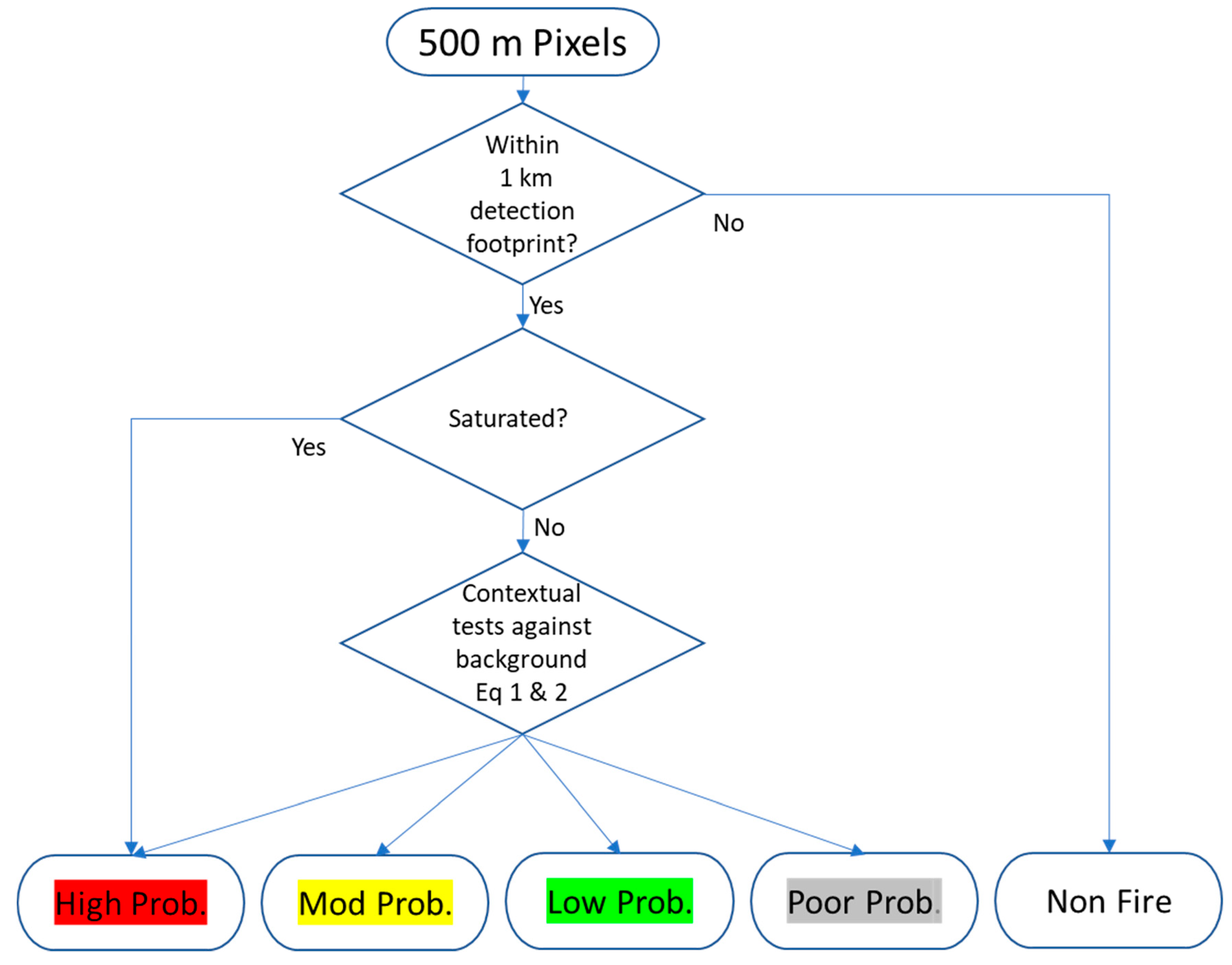
The downscaling algorithm is a straightforward adaptation of the established active fire detection techniques using reflective bands [10,35,36,37,38]. Initially, all 500 m pixels that are encompassed within the 1 km detection pixel footprint are considered fire candidates. The 500 m pixels that are outside the detection footprint but within 1 km are considered to be adjacent to fire pixels that may be contaminated with non-detected active fire components. All 500 m pixels encompassed by a 1 km pixel identified as water are all conservatively labeled as water and cloudy pixels are ignored [35,37]. The probability classes for each of the 500 m candidate fire pixels are assigned using the Figure 1 flowchart and the following tests.
If the fire candidate pixel’s 2.13 μm band 7 reflectance is saturated ( it is assigned the highest probability class for presence of active fire. Saturation of the 2 μm bands in moderate resolution satellites such as Landsat occurs only over fires or over highly reflective surfaces that can cause sun glint under the right illumination geometry [35,37,50]. Since the saturated candidate 500 m pixel is within a 1 km pixel already known to encompass an actively burning fire, it is assigned the highest probability class and is not a bright reflective surface.
All remaining 500 m candidate fire pixels are further examined through a contextual test to assign their probability class for presence of active fires, by comparing their reflectance values with their corresponding background pixel value, similar to the approach used in the MODIS active fire detection algorithm [2,35,37]. The background pixels are selected from a square window centered on the candidate fire pixel. The window starts as a 7 × 7 pixel square ring and is grown spirally to include 9 × 9, 11 × 11, 13 × 13 ….to a maximum of 31 × 31 pixels until at least 25% of the pixels within the window are non-fire, non-candidate, non-saturated, not adjacent to fire and non-water pixels, and the selected number is at least 32 [2,35]. The mean and standard deviation values are calculated using the selected background pixel’s 2.13 μm band reflectance values and the ratio of 2.13 μm band reflectance to the 0.87 μm band reflectance. These are compared [35,37] to the candidate’s 2.13 μm band reflectance and the ratio of 2.13 μm band reflectance to the 0.87 μm band reflectance as Equations (1) and (2).
And
where the is the reflectance in the spectral band noted in the subscripts of the candidate 500 m fire pixel, and x represent the mean and standard deviation respectively of the selected × neighbors. The n in the above equations define the breaks for the probability classes.
For example, the (highest probability) criterion is when and . Similarly, the < (moderate) < (low) and < (poor) 500 m active fire probability is assigned.
Downscaling coarse resolution to finer resolution is often not encouraged [51] due to band-to-band registration mismatches. However, since the downscaling algorithm presented in this work is only a relative comparison of ratios between candidate pixel and their neighborhood with locally adaptive thresholds, errors due to resampling and band-to-band misregistration are expected to be minimal. Furthermore, more recent research [52] reported the band-to-band registration error was expected to be less than 0.1% for MODIS.
3.2. Accuracy Assessment
Validation of satellite active fire detection is challenging due to difficulties in obtaining independent reference data at the time of over pass. Past satellite active fire detection validation studies [36,38,53] used concurrent high-resolution (30 m) ASTER satellite active fire detections for validations. Satellite reflectance-based active fire detections have been validated by examining higher resolution imagery of active fire locations and expert opinion [35,37]. In this work we follow a similar methodology for accuracy assessments of the algorithm performance over two test sites. We use available ASTER and Google Earth™ images and examine 500 m locations for the presence/absence of active fire for accuracy assessments. Results of this analysis are not representative of global performance of the algorithm.
3.2.1. Gas Flares
Gas flares are typically hotter (>1600 K) [54] compared to ~1000 K flaming vegetation fires [2,55] and hence are easily identifiable in thermal imagery. Gas flare stacks (active and inactive) are also easily visible in high-resolution visual band imagery, enabling the pinpointing of the exact location of the source. However, not all gas flares are detected by MODIS [56,57], as the MODIS daytime active fire algorithm is more sensitive to larger biomass fires. Therefore, only those MODIS tiles on specific dates when active fires were detected over the gas flare sites by the MODIS daytime active fire algorithm and that were also cloud free were selected. We selected Iraqi gas stack locations as they are numerous and are surrounded by desert with sparse vegetation. The locations of gas flares are visually identified and are compared to their assigned probabilities for assessment. Gas flares are expected to be located predominantly within the highest probability pixels, while pixels with low probabilities may occur around high probability pixels but away from known gas flare locations. However, construction development (commissioning and/or decommissioning of existing gas flares with respect to base imagery and date of active fire detection), prevailing wind direction, physical size of the fire and viewing geometry depending on the height of the fire stack and point spread function of the MODIS sensors may cause more than one 500 m pixel to be flagged as high probability. Considering all these sources of error, the distribution of probabilities and the presence or absence of gas flares in the 500 m pixels is visually judged, tabulated, and discussed. Table 1 presents the data used for examining the gas flares.
3.2.2. Wildfire
Quantitative validation of MODIS active fire products for detecting wildfire has been demonstrated using concurrent 30 m ASTER observations [36,38]. We follow a similar methodology and use MODIS Terra observations and concurrent observations by ASTER over an African savanna fire. A simple thresholding algorithm [36] on the 30 m Channel 9 ASTER, where 2 μm radiance > 6.33 W m2 sr−2 μm−1, to classify 30 m ASTER active fire pixels as burning. The 30 m ASTER fire pixels in each of the 500 m MODIS subpixels are examined considering their assigned probabilities.
Accuracy was also qualitatively inferred by visual examination of the distribution of 500 m pixels within the 1 km detector footprint and their active fire presence probabilities over the largest and recent (27 July 2018 Ranch fire in California) wildfire in the United States using available high-resolution imagery. Accuracy of 500 m pixel probabilities and the wildfire perimeter that is visible within high-resolution imagery (see Table 1 for high-resolution imagery sources) is visually evaluated.
4. Results
4.1. Gas Flares Results
The 2019 MOD14A2 H22V05 tile had a total of 116 (1 km) active fire detections on 1 February (DOY 32) that could be visually grouped as 29 contiguous clusters. Clusters over agricultural fields and industrial units that are spread over multiple 500 m pixels with no obvious distinct source such as a flare stack or active gas flare are excluded from this study. These are not MODIS commission errors but are detections where the fire could have occurred anywhere, and its location cannot be reliably determined by using non-concurrent imagery. Out of the 29 clusters only 19 had obvious flare stacks (active and inactive in the time of base imagery) in the most recent images (2010 base imagery compared to 2019 active fire detection) available on Google Earth™. Table 2 shows the number of 500 m pixels that belong to a particular probability class for each of the 19 cluster of detections over gas flares after the application of the downscaling algorithm. Downscaled 500 m pixels that had more than one flare stack (active or inactive) are shown in bold. It is evident that flare stacks were seen mostly in the pixels that are assigned the highest probability classes and conversely the lower probability classes have the least chance of containing a flare stack within their footprint. No visual evidence of flare stacks in any of the poor probability pixels in all 19 clusters analyzed is seen. However, there were few (Table 2: cluster id 7, 9, 13, 19) instances where flare stacks were visually identified outside the high probability class 500 m pixels. In all of these cases, at least one flare stack is seen within 150 m of high probability pixel boundaries. Over the Iraqi gas flare test site 84% (16/19) of the highest and moderate probability contiguous 500 pixels had at least one flare stack in them while 16% (3/19) of clusters had evident flare stacks in the low probability pixels
An illustrative example of the performance of the downscaling algorithm over a gas flare (Cluster ID #2: Table 2) is shown in Figure 2. It is evident that the highest probability pixels encompass the visibly burning flare stacks. High probability pixels with no flare stacks evident are also seen adjacent to high probability pixels with no evident flare stack. This may be due to a combination of effects including the height of the flare stack and view angle, newer construction, geolocation errors, sensor point spread functions, and atmospheric effects [35,37], including prevailing wind. No flare stacks (either active or inactive) are visible in the lower probability pixels. A pixel with no flare stack has also been assigned a moderate probability by the algorithm. However, as discussed above, such commission errors for adjacent pixels are expected.
4.2. Wildfire Results
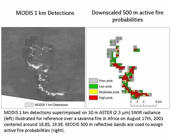
MODIS 1 km active fire detections overlapping with ASTER imagery over a savanna in Africa on 17 August 2001 are illustrated in Figure 3. A total of 72 MODIS 1 km active fire detections were observed over the overlapping region. Application of the downscaling algorithm resulted in consideration of 290 candidate 500 m pixels. Out of these 85 were assigned the highest probability, 27 moderate, 77 low, and 101 poor probability class by the downscaling algorithm. The 30 m ASTER fire detections and the 30 m ASTER Channel 9 (2 μm) along with the 15 m ASTER NIR Channel 3N (0.8 μm) to highlight the smoke in the southwest (Figure 3) are also shown for reference. The high and medium probability 500 m pixels encompass obvious actively flaming fire fronts within the ASTER active fire detections. Similar to the observations over the Iraqi gas flares, the high and medium probability pixels evidently show actively flaming fire fronts. In fact, 73/85 (85%) high and 22/27 (81%) and moderate probability pixels had at least one ASTER detection pixel, respectively. Overall about 85% of the high and moderate pixels had at least one ASTER 30 m active fire detection pixel. Low and poor probability pixels do not exhibit any visually obvious actively flaming fronts within the reflective band observations. About 42% and 6% of the low and poor probability pixels, respectively had at least one ASTER 30 m detection. Omission errors are also visually evident in the imagery that may be due to the difference in the fractional fire size as compared to the observation pixel, or from smoke/cloud obscuration. These results and summaries are image-specific and are not representative of global performance of the algorithm or MODIS active fire detection sensitivity.
Figure 4 illustrates application of the downscaling algorithm over the Ranch wildland fire in the United States on 4 August 2018, superimposed on a high-resolution base imagery that was acquired before and after the fire. The fire continued to burn beyond the illustrated day of detection and continued to move towards the northwest. It is evident that the area under the high probability pixels exhibit visible burn scars, while areas with lower probabilities over the dry riverbed show no burn scar. Visible burn scars in the low probability pixels perhaps resulted from fires that occurred after 4 August 2018 and before 15 August 2018 when the base imagery was acquired
The performance of the downscaling algorithm under clear versus cloudy sky conditions on different days is shown in Figure 5. This is the same wildland fire shown in Figure 4 but covering a larger spatial extent (150 × 150 km) and encompassing the whole fire. Left panels show a false color image using red (2.13 μm), green (0.85 μm), and blue (0.64 μm) band combinations. Top left panel shows MODIS acquisitions are on a clear day. As expected the highest probability pixels are clustered near the center of the polygons surrounded by pixels with lower probabilities. This is expected because the interior fire cores are hotter and so have higher radiance than at the periphery, and because fire periphery pixels are more likely to include cooler non-burning surfaces [35]. It is evident that the algorithm performs well during clear sky conditions by clearly delineating active fire fronts; however, if the pixels are obscured by clouds and haze they are assigned low probabilities. The algorithm is dependent on not just the 2.13 μm (SWIR) band but also the 0.85 μm (NIR) band that is sensitive to smoke and aerosols, which can obstruct viewing of flaming fronts in these wavelengths.
5. Discussion
This work presents the development of a downscaled 500 m active fire product using the 1 km MODIS Aqua and Terra daytime detections. The algorithm leverages reflectance-based active fire detection techniques and adapts established algorithms to assign probability class pixels within the 1 km MODIS active fire detection footprint. Performance of the active fire algorithms is assessed quantitatively and qualitatively using detections over static gas flares and over wildland fires. Over 84% of MODIS active fire detections with evident actively flaming fronts or flare stacks were correctly assigned to the high probability class in the two sites examined in this study. The algorithm also assigned low probability values to pixels with no clear evidence of active fires in any of the 500 m subpixels. Visual inspection of the spatial distribution of the 500 m downscaled pixels suggest that the highest probability pixels are clustered near the center and are surrounded by pixels with lower probabilities. This is expected behavior of active fire detection algorithm given that the fire interior cores are hotter and have higher radiance values as compared to the fire periphery, and that the fire periphery pixels are more likely to include cooler non-burning surfaces [35]. Results clearly indicate that the algorithm performs well under clear sky conditions for our selected test sites.
The performance of the algorithm may be influenced by the relative distribution of fire sizes and temperatures within the detector footprint. Simulations [36] have shown that even a small fire (0.5% of pixel footprint) burning at a high flaming temperature will show significant SWIR elevation; however, such effects are less pronounced for large fires that are smoldering at lower temperatures. The performance of the active fire detection algorithm is further impacted by atmospheric effects including scattering, obscuration, and may be limited by sensor characteristics including geolocation errors, and sensor point spread functions. It should be noted that MODIS’s off nadir active fires observation footprints are much larger and can detect only sufficiently hot and large fires [9,58,59]. The subsequent resampling to 1 km in the Level 3 product may introduce errors of commission and can influence this downscaling algorithm. Irrespective of the pixel size, the downscaling algorithm has the potential to reduce the spatial uncertainty to half of the original footprint. This can be seen in Figure 5 (bottom) where despite the larger pixels size (lower spatial detail even in cloud free regions) in the off-nadir observations, the downscaling algorithm reduces the spatial uncertainty when possible. Although the downscaling algorithm can only improve fire location probabilities under clear day conditions, the sensitivity of the downscaled active fire product is the same (50% probability of detection for ~100 m2, flaming ~1000 K) as for the 1 km active fire detection of the MODIS 1 km detections [2,45].
6. Conclusions
A downscaled active fire product can potentially reduce the location and area uncertainty by one half and one fourth respectively is derived using the operational 1 km product. The algorithm is applicable to both MODIS and the Sentinel 3 A and B satellites that are currently in orbit. The Sentinel satellites have the required 1 km 3.7 μm emissive band (S7, F1) for active fire detection capability [34] and the reflective 500 m 2.2 μm band (S6) and a 0.86 μm band (S3) [33] required for downscaling. It is expected that the downscaling algorithm could be directly applicable to the Sentinel 3 A and B satellites although they have slightly different central wavelengths (2.25 μm, 0.86 μm) and spectral response as compared to MODIS. This direct applicability is expected because thresholds used in this algorithm are locally adaptive and are relative to their neighbors. This can potentially augment the twice daily MODIS active fire data globally.
This downscaled product will find use for near real-time application by first responders and fire management personnel who need active fire maps with enhanced spatial resolution and will also prove useful for researchers in the fire science community. Active fire detections have been shown to be correlated [41] well with burned area and such downscaled active fire product may find immediate application in such studies. Furthermore, improved spatial resolution will help studies investigating and monitoring active fire locations and its proximities to wildland urban interfaces [60]. Currently, within the United States there are three national burn mapping projects that could potentially benefit from the higher spatial resolution active fire mapping, including the Monitoring Trends in Burn Severity (MTBS) [61], Burned Area Essential Climate Variable (BAECV) [62], and LANDFIRE [63]. MTBS currently uses the Integrated Reporting of Wildland Fire Information (IRWIN) [64] database to access geospatially referenced wildland fire locations. The IRWIN database reduces the amount of duplication in fire reporting, but because it is dependent on government agencies reporting fires, it can miss fires in areas where fires are not regularly reported. Underrepresented fires can be especially problematic where there are large amounts of prescribed fires on nonfederal lands. MTBS could potentially integrate the downscaled active fire product into its mapping to better separate large burned areas present within the central and southeastern US. MTBS does not map all fires on nonfederal lands and only fires that are greater than 404 ha in the western and greater than 202 ha in the eastern US. The BAECV data products attempt to map all fires visible in Landsat 30 m imagery within the conterminous United States [62]. Although the BAECV burned area product has reasonable accuracy there are some potential problems with commission errors [65]. These commission errors could potentially be reduced, by considering only those BAECV burned areas that intersect active fire detection footprints with high probabilities. Both MTBS and BAECV are incorporated into the LANDFIRE disturbance mapping process [66], with MTBS used as a disturbance and BAECV used to inform disturbance causality (i.e., fire). The coarse resolution of the active fire detection makes it unlikely that it will be used as a disturbance layer such as MTBS; however, downscaled MODIS and Sentinel 3 active fire detections could be used similarly to BAECV by informing LANDFIRE disturbance causality.
Author Contributions
Conceptualization, S.S.K.; Methodology, S.S.K., J.J.P. and B.P.; Writing—original draft, S.S.K.; Writing—review and editing, J.J.P. and B.P.
Funding
This work was performed under the US. Geological Survey (USGS) contract #140G0119C0001.
Acknowledgments
We thank Manohar Velpuri, Sandra Cooper, and the three anonymous reviewers whose comments and suggestions greatly improved our manuscript. All the data used in this study were obtained from public domains and are freely available. Any use of trade, firm, or product names is for descriptive purposes only and does not imply endorsement by the US Government.
Conflicts of Interest
The authors declare no conflict of interest. The funders had no role in the design of the study; in the collection, analyses, or interpretation of data; in the writing of the manuscript, or in the decision to publish the results.
References
- Davies, A.; Chien, S.; Baker, V.; Doggett, T.; Dohm, J.; Greeley, R.; Ip, F.; Castan, R.; Cichy, B.; Rabideau, G. Monitoring active volcanism with the autonomous sciencecraft experiment on EO-1. Remote Sens. Environ. 2006, 101, 427–446. [Google Scholar] [CrossRef]
- Giglio, L.; Descloitres, J.; Justice, C.O.; Kaufman, Y.J. An enhanced contextual fire detection algorithm for MODIS. Remote Sens. Environ. 2003, 87, 273–282. [Google Scholar] [CrossRef]
- Matson, M.; Dozier, J. Identification of subresolution high temperature sources using a thermal IR sensor. Photogramm. Eng. Remote Sens. 1981, 47, 1311–1318. [Google Scholar]
- Prins, E.M.; Menzel, W.P. Geostationary satellite detection of bio mass burning in South America. Int. J. Remote Sens. 1992, 13, 2783–2799. [Google Scholar] [CrossRef]
- Robinson, J.M. Fire from space: Global fire evaluation using infrared remote sensing. Int. J. Remote Sens. 1991, 12, 3–24. [Google Scholar] [CrossRef]
- Aragao, L.E.O.; Malhi, Y.; Roman-Cuesta, R.M.; Saatchi, S.; Anderson, L.O.; Shimabukuro, Y.E. Spatial patterns and fire response of recent Amazonian droughts. Geophys. Res. Lett. 2007, 34. [Google Scholar] [CrossRef] [Green Version]
- Chuvieco, E.; Giglio, L.; Justice, C. Global characterization of fire activity: Toward defining fire regimes from Earth observation data. Glob. Change Biol. 2008, 14, 1488–1502. [Google Scholar] [CrossRef]
- Giglio, L. Characterization of the tropical diurnal fire cycle using VIRS and MODIS observations. Remote Sens. Environ. 2007, 108, 407–421. [Google Scholar] [CrossRef]
- Loboda, T.; Csiszar, I. Reconstruction of fire spread within wildland fire events in Northern Eurasia from the MODIS active fire product. Glob. Planet. Change 2007, 56, 258–273. [Google Scholar] [CrossRef]
- Schroeder, W.; Morisette, J.T.; Csiszar, I.; Giglio, L.; Morton, D.; Justice, C.O. Characterizing vegetation fire dynamics in Brazil through multisatellite data: Common trends and practical issues. Earth Interact. 2005, 9, 1–26. [Google Scholar] [CrossRef]
- Boschetti, L.; Roy, D.P. Defining a fire year for reporting and analysis of global interannual fire variability. J. Geophys. Res. Biogeosci. 2008, 113. [Google Scholar] [CrossRef] [Green Version]
- Kumar, S.S.; Roy, D.P.; Cochrane, M.A.; Souza, C.M.; Barber, C.P.; Boschetti, L. A quantitative study of the proximity of satellite detected active fires to roads and rivers in the Brazilian tropical moist forest biome. Int. J. Wildland Fire 2014, 23, 532–543. [Google Scholar] [CrossRef]
- Pereira, J.M.; Oom, D.; Pereira, P.; Turkman, A.A.; Turkman, K.F. Religious affiliation modulates weekly cycles of cropland burning in sub-Saharan Africa. PLoS ONE 2015, 10, e0139189. [Google Scholar] [CrossRef]
- Bowman, D.M.; Balch, J.K.; Artaxo, P.; Bond, W.J.; Carlson, J.M.; Cochrane, M.A.; D’Antonio, C.M.; DeFries, R.S.; Doyle, J.C.; Harrison, S.P. Fire in the Earth system. Science 2009, 324, 481–484. [Google Scholar] [CrossRef] [PubMed]
- Lentile, L.B.; Holden, Z.A.; Smith, A.M.; Falkowski, M.J.; Hudak, A.T.; Morgan, P.; Lewis, S.A.; Gessler, P.E.; Benson, N.C. Remote sensing techniques to assess active fire characteristics and post-fire effects. Int. J. Wildland Fire 2006, 15, 319–345. [Google Scholar] [CrossRef]
- Oppenheimer, C. Lava flow cooling estimated from Landsat Thematic Mapper infrared data: The Lonquimay eruption (Chile, 1989). J. Geophys. Res. Solid Earth 1991, 96, 21865–21878. [Google Scholar] [CrossRef]
- Murphy, S.W.; de Souza Filho, C.R.; Wright, R.; Sabatino, G.; Pabon, R.C. HOTMAP: Global hot target detection at moderate spatial resolution. Remote Sens. Environ. 2016, 177, 78–88. [Google Scholar] [CrossRef]
- Kaiser, J.; Heil, A.; Andreae, M.; Benedetti, A.; Chubarova, N.; Jones, L.; Morcrette, J.; Razinger, M.; Schultz, M.; Suttie, M. Biomass burning emissions estimated with a global fire assimilation system based on observed fire radiative power. Biogeosciences 2012, 9, 527–554. [Google Scholar] [CrossRef] [Green Version]
- Zhang, X.; Kondragunta, S.; Roy, D.P. Interannual variation in biomass burning and fire seasonality derived from Geostationary satellite data across the contiguous United States from 1995 to 2011. J. Geophys. Res. Biogeosci. 2014, 119, 1147–1162. [Google Scholar] [CrossRef]
- Anderson, K.R.; Englefield, P.; Little, J.; Reuter, G. An approach to operational forest fire growth predictions for Canada. Int. J. Wildland Fire 2010, 18, 893–905. [Google Scholar] [CrossRef]
- Davies, D.K.; Ilavajhala, S.; Wong, M.M.; Justice, C.O. Fire information for resource management system: Archiving and distributing MODIS active fire data. IEEE Trans. Geosci. Remote Sens. 2009, 47, 72–79. [Google Scholar] [CrossRef]
- Trigg, S.; Flasse, S. Characterizing the spectral-temporal response of burned savannah using in situ spectroradiometry and infrared thermometry. Int. J. Remote Sens. 2000, 21, 3161–3168. [Google Scholar] [CrossRef]
- Boschetti, L.; Roy, D.P.; Justice, C.O.; Humber, M.L. MODIS–Landsat fusion for large area 30 m burned area mapping. Remote Sens. Environ. 2015, 161, 27–42. [Google Scholar] [CrossRef]
- Fraser, R.; Li, Z.; Cihlar, J. Hotspot and NDVI differencing synergy (HANDS): A new technique for burned area mapping over boreal forest. Remote Sens. Environ. 2000, 74, 362–376. [Google Scholar] [CrossRef]
- Giglio, L.; Loboda, T.; Roy, D.P.; Quayle, B.; Justice, C.O. An active-fire based burned area mapping algorithm for the MODIS sensor. Remote Sens. Environ. 2009, 113, 408–420. [Google Scholar] [CrossRef]
- Roy, D.P. Multi-temporal active-fire based burn scar detection algorithm. Int. J. Remote Sens. 1999, 20, 1031–1038. [Google Scholar] [CrossRef]
- Hyer, E.J.; Reid, J.S. Baseline uncertainties in biomass burning emission models resulting from spatial error in satellite active fire location data. Geophys. Res. Lett. 2009, 36. [Google Scholar] [CrossRef]
- Roy, D.P.; Kumar, S.S. Multi-year MODIS active fire type classification over the Brazilian Tropical Moist Forest Biome. Int. J. Digit. Earth 2017, 10, 54–84. [Google Scholar] [CrossRef]
- Ten Hoeve, J.; Remer, L.; Correia, A.L.; Jacobson, M. Recent shift from forest to savanna burning in the Amazon Basin observed by satellite. Environ. Res. Lett. 2012, 7, 024020. [Google Scholar] [CrossRef]
- Morton, D.; Defries, R.; Randerson, J.; Giglio, L.; Schroeder, W.; Van Der Werf, G. Agricultural intensification increases deforestation fire activity in Amazonia. Glob. Change Biol. 2008, 14, 2262–2275. [Google Scholar] [CrossRef] [Green Version]
- Schroeder, W.; Oliva, P.; Giglio, L.; Csiszar, I.A. The New VIIRS 375 m active fire detection data product: Algorithm description and initial assessment. Remote Sens. Environ. 2014, 143, 85–96. [Google Scholar] [CrossRef]
- Oliva, P.; Schroeder, W. Assessment of VIIRS 375 m active fire detection product for direct burned area mapping. Remote Sens. Environ. 2015, 160, 144–155. [Google Scholar] [CrossRef]
- Donlon, C.; Berruti, B.; Buongiorno, A.; Ferreira, M.H.; Féménias, P.; Frerick, J.; Goryl, P.; Klein, U.; Laur, H.; Mavrocordatos, C.; et al. The Global Monitoring for Environment and Security (GMES) Sentinel-3 mission. Remote Sens. Environ. 2012, 120, 37–57. [Google Scholar] [CrossRef]
- Wooster, M.J.; Xu, W.; Nightingale, T. Sentinel-3 SLSTR active fire detection and FRP product: Pre-launch algorithm development and performance evaluation using MODIS and ASTER datasets. Remote Sens. Environ. 2012, 120, 236–254. [Google Scholar] [CrossRef]
- Kumar, S.S.; Roy, D.P. Global operational land imager Landsat-8 reflectance-based active fire detection algorithm. Int. J. Digit. Earth 2018, 11, 154–178. [Google Scholar] [CrossRef]
- Morisette, J.T.; Giglio, L.; Csiszar, I.; Justice, C.O. Validation of the MODIS active fire product over Southern Africa with ASTER data. Int. J. Remote Sens. 2005, 26, 4239–4264. [Google Scholar] [CrossRef]
- Schroeder, W.; Oliva, P.; Giglio, L.; Quayle, B.; Lorenz, E.; Morelli, F. Active fire detection using Landsat-8/OLI data. Remote Sens. Environ. 2016, 185, 210–220. [Google Scholar] [CrossRef] [Green Version]
- Schroeder, W.; Prins, E.; Giglio, L.; Csiszar, I.; Schmidt, C.; Morisette, J.; Morton, D. Validation of GOES and MODIS active fire detection products using ASTER and ETM+ data. Remote Sens. Environ. 2008, 112, 2711–2726. [Google Scholar] [CrossRef]
- Coen, J.L.; Schroeder, W. Use of spatially refined satellite remote sensing fire detection data to initialize and evaluate coupled weather-wildfire growth model simulations. Geophys. Res. Lett. 2013, 40, 5536–5541. [Google Scholar] [CrossRef]
- Massada, A.B.; Syphard, A.D.; Hawbaker, T.J.; Stewart, S.I.; Radeloff, V.C. Effects of ignition location models on the burn patterns of simulated wildfires. Environ. Model. Softw. 2011, 26, 583–592. [Google Scholar] [CrossRef]
- Hantson, S.; Padilla, M.; Corti, D.; Chuvieco, E. Strengths and weaknesses of MODIS hotspots to characterize global fire occurrence. Remote Sens. Environ. 2013, 131, 152–159. [Google Scholar] [CrossRef]
- Wolfe, R.E.; Nishihama, M.; Fleig, A.J.; Kuyper, J.A.; Roy, D.P.; Storey, J.C.; Patt, F.S. Achieving sub-pixel geolocation accuracy in support of MODIS land science. Remote Sens. Environ. 2002, 83, 31–49. [Google Scholar] [CrossRef]
- Wolfe, R.E.; Roy, D.P.; Vermote, E. MODIS land data storage, gridding, and compositing methodology: Level 2 grid. IEEE Trans. Geosci. Remote Sens. 1998, 36, 1324–1338. [Google Scholar] [CrossRef] [Green Version]
- Justice, C.O.; Vermote, E.; Townshend, J.R.; Defries, R.; Roy, D.P.; Hall, D.K.; Salomonson, V.V.; Privette, J.L.; Riggs, G.; Strahler, A. The Moderate Resolution Imaging Spectroradiometer (MODIS): Land remote sensing for global change research. IEEE Trans. Geosci. Remote Sens. 1998, 36, 1228–1249. [Google Scholar] [CrossRef]
- Giglio, L.; Schroeder, W.; Justice, C.O. The collection 6 MODIS active fire detection algorithm and fire products. Remote Sens. Environ. 2016, 178, 31–41. [Google Scholar] [CrossRef] [Green Version]
- Wolfe, R.E.; Roy, D.P. The MODIS land data storage methodology: Level 2 grid. In Proceedings of the IGARSS’98. Sensing and Managing the Environment. 1998 IEEE International Geoscience and Remote Sensing. Symposium Proceedings. (Cat. No. 98CH36174), Seattle, WA, USA, 6–10 July 1998; pp. 1585–1589. [Google Scholar]
- EARTHDATA. Available online: https://earthdata.nasa.gov/ (accessed on 1 March 2019).
- Freeborn, P.H.; Wooster, M.J.; Roy, D.P.; Cochrane, M.A. Quantification of MODIS fire radiative power (FRP) measurement uncertainty for use in satellite-based active fire characterization and biomass burning estimation. Geophys. Res. Lett. 2014, 41, 1988–1994. [Google Scholar] [CrossRef]
- Yamaguchi, Y.; Kahle, A.B.; Tsu, H.; Kawakami, T.; Pniel, M. Overview of advanced spaceborne thermal emission and reflection radiometer (ASTER). IEEE Trans. Geosci. Remote Sens. 1998, 36, 1062–1071. [Google Scholar] [CrossRef]
- Morfitt, R.; Barsi, J.; Levy, R.; Markham, B.; Micijevic, E.; Ong, L.; Scaramuzza, P.; Vanderwerff, K. Landsat-8 Operational Land Imager (OLI) radiometric performance on-orbit. Remote Sens. 2015, 7, 2208–2237. [Google Scholar] [CrossRef]
- Tan, B.; Woodcock, C.; Hu, J.; Zhang, P.; Ozdogan, M.; Huang, D.; Yang, W.; Knyazikhin, Y.; Myneni, R. The impact of gridding artifacts on the local spatial properties of MODIS data: Implications for validation, compositing, and band-to-band registration across resolutions. Remote Sens. Environ. 2006, 105, 98–114. [Google Scholar] [CrossRef]
- Xie, Y.; Xiong, X.; Qu, J.J.; Che, N.; Summers, M.E. Impact analysis of MODIS band-to-band registration on its measurements and science data products. Int. J. Remote Sens. 2011, 32, 4431–4444. [Google Scholar] [CrossRef]
- Giglio, L.; Csiszar, I.; Restás, Á.; Morisette, J.T.; Schroeder, W.; Morton, D.; Justice, C.O. Active fire detection and characterization with the advanced spaceborne thermal emission and reflection radiometer (ASTER). Remote Sens. Environ. 2008, 112, 3055–3063. [Google Scholar] [CrossRef]
- Fisher, D.; Wooster, M. Shortwave IR Adaption of the Mid-Infrared Radiance Method of Fire Radiative Power (FRP) Retrieval for Assessing Industrial Gas Flaring Output. Remote Sens. 2018, 10, 305. [Google Scholar] [CrossRef]
- Kaufman, Y.J.; Justice, C.O.; Flynn, L.P.; Kendall, J.D.; Prins, E.M.; Giglio, L.; Ward, D.E.; Menzel, W.P.; Setzer, A.W. Potential global fire monitoring from EOS-MODIS. J. Geophys. Res. Atmos. 1998, 103, 32215–32238. [Google Scholar] [CrossRef]
- Anejionu, O.C.; Blackburn, G.A.; Whyatt, J.D. Detecting gas flares and estimating flaring volumes at individual flow stations using MODIS data. Remote Sens. Environ. 2015, 158, 81–94. [Google Scholar] [CrossRef] [Green Version]
- Elvidge, C.D.; Baugh, K.E.; Ziskin, D.; Anderson, S.; Ghosh, T. Estimation of Gas Flaring Volumes Using NASA MODIS Fire Detection Products; Annual Report; NOAA National Geophysical Data Center (NGDC): Boulder, CO, USA, 2011.
- Kumar, S.; Roy, D.P.; Boschetti, L.; Kremens, R. Exploiting the power law distribution properties of satellite fire radiative power retrievals: A method to estimate fire radiative energy and biomass burned from sparse satellite observations. J. Geophys. Res. Atmos. 2011, 116. [Google Scholar] [CrossRef] [Green Version]
- Boschetti, L.; Roy, D.P. Strategies for the fusion of satellite fire radiative power with burned area data for fire radiative energy derivation. J. Geophys. Res. Atmos. 2009, 114. [Google Scholar] [CrossRef] [Green Version]
- Ahmed, M.; Rahaman, K.; Hassan, Q. Remote sensing of wildland fire-induced risk assessment at the community level. Sensors 2018, 18, 1570. [Google Scholar] [CrossRef]
- Eidenshink, J.; Schwind, B.; Brewer, K.; Zhu, Z.-L.; Quayle, B.; Howard, S. A project for monitoring trends in burn severity. Fire Ecol. 2007, 3, 3–21. [Google Scholar] [CrossRef]
- Hawbaker, T.J.; Vanderhoof, M.K.; Beal, Y.-J.; Takacs, J.D.; Schmidt, G.L.; Falgout, J.T.; Williams, B.; Fairaux, N.M.; Caldwell, M.K.; Picotte, J.J. Mapping burned areas using dense time-series of Landsat data. Remote Sens. Environ. 2017, 198, 504–522. [Google Scholar] [CrossRef]
- Rollins, M.G. LANDFIRE: A nationally consistent vegetation, wildland fire, and fuel assessment. Int. J. Wildland Fire 2009, 18, 235–249. [Google Scholar] [CrossRef]
- IRWIN. Integerated Reporting of Wildland-Fire Information (IRWIN). Available online: https://www.forestsandrangelands.gov/WFIT/applications/IRWIN/index.shtml (accessed on 1 March 2019).
- Vanderhoof, M.K.; Fairaux, N.; Beal, Y.-J.G.; Hawbaker, T.J. Validation of the USGS Landsat burned area essential climate variable (BAECV) across the conterminous United States. Remote Sens. Environ. 2017, 198, 393–406. [Google Scholar] [CrossRef]
- LANDFIRE. Update Disturbance Dataset. Available online: https://landfire.gov/disturbance.php (accessed on 1 March 2019).
Figure 1.
Downscaling algorithm flowchart.

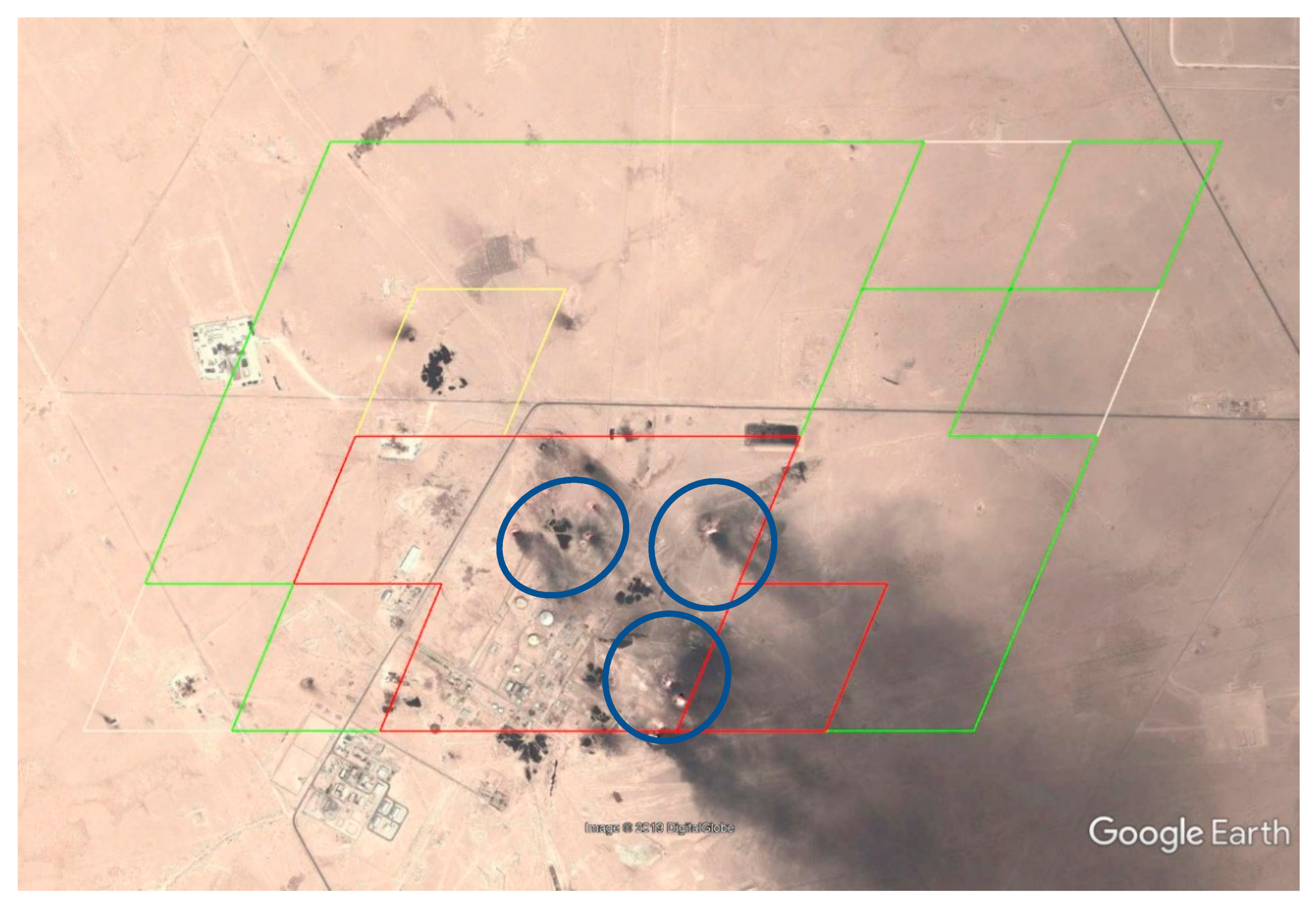
Figure 2.
Illustrative proof of concept results over gas flares in Iraq (centered at N 30.216575, E 47.39269). Background Google Earth™ image was acquired on 31 August 2010 while the overlaid pixels are all 500 m pixels within the six 1 km detection footprint detected on 1 February 2019, DOY 032. Colored boundary lines outline the area encompassed by nine 1 km active detection pixels (Table 1, Cluster ID 2). Colored outlines mark the high (red), moderate (yellow) and low (green) and poor (white) probabilities of subpixels containing active fire(s). Gas flares (within blue ovals) are evidently closest to the contiguous high probability locations and further away from the poor probability locations. Out of the six contiguous high probability pixels three do not have any obvious flare stack.

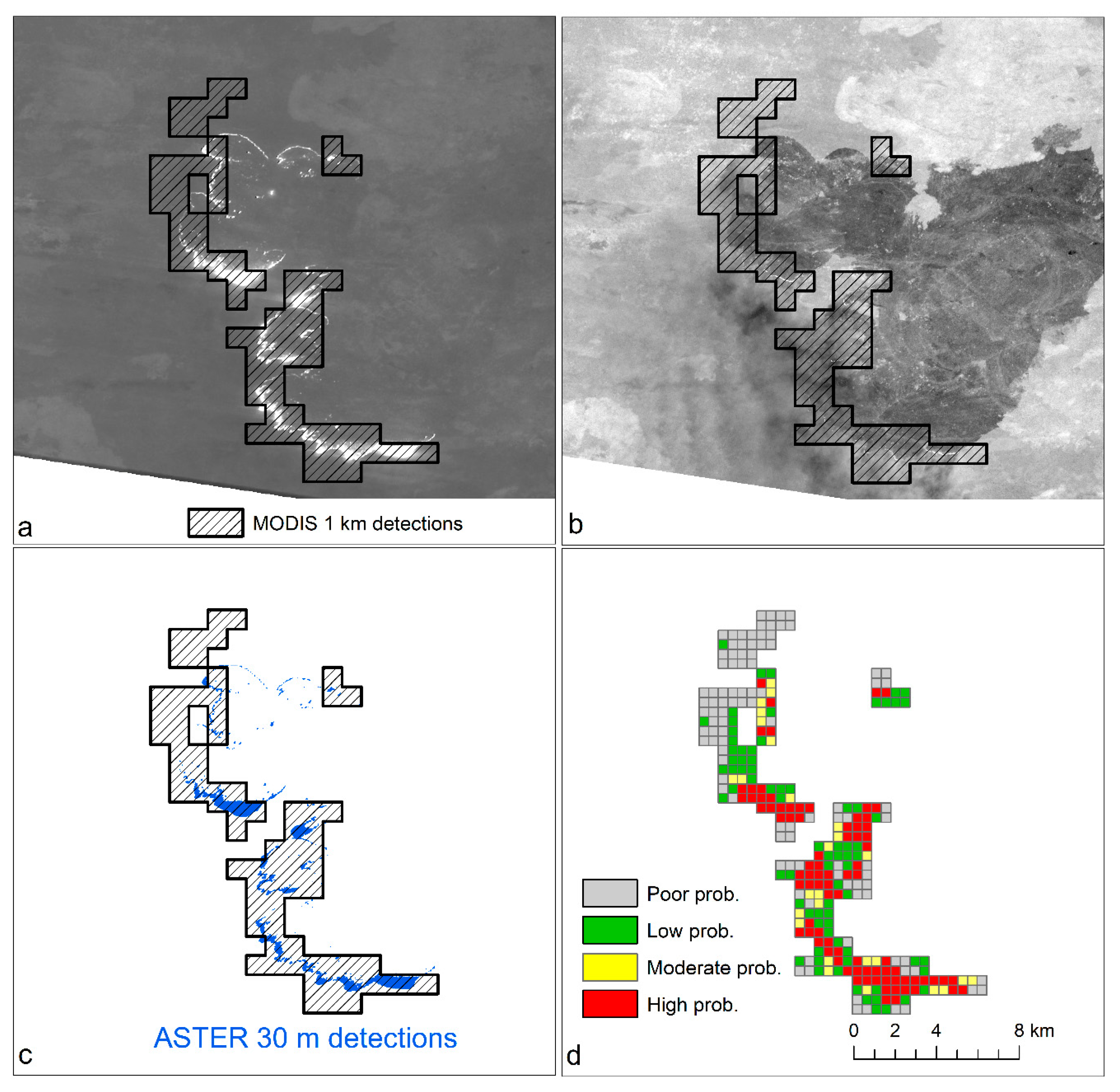
Figure 3.
Proof of concept results over a savanna fire in Africa on 17 August 2001, DOY 229. Illustrated (a) 30 m ASTER Channel 9 (2.3 μm) SWIR radiance with MODIS 1 km (crosshatched) detections. (b) 15 m ASTER Channel 3N (0.8 μm) NIR reflectance. (c) ASTER fire detections (blue) superimposed with MODIS 1 km detections. (d) Results of this work, pixels colored by their probability classes (high (red), moderate (yellow) and low (green) and poor (gray)). Flaming fronts are visible within the MODIS 500 m pixels shaded red and yellow. No flaming fronts/ASTER fire detections are evident in the MODIS poor (green) and low (gray) probability pixels.

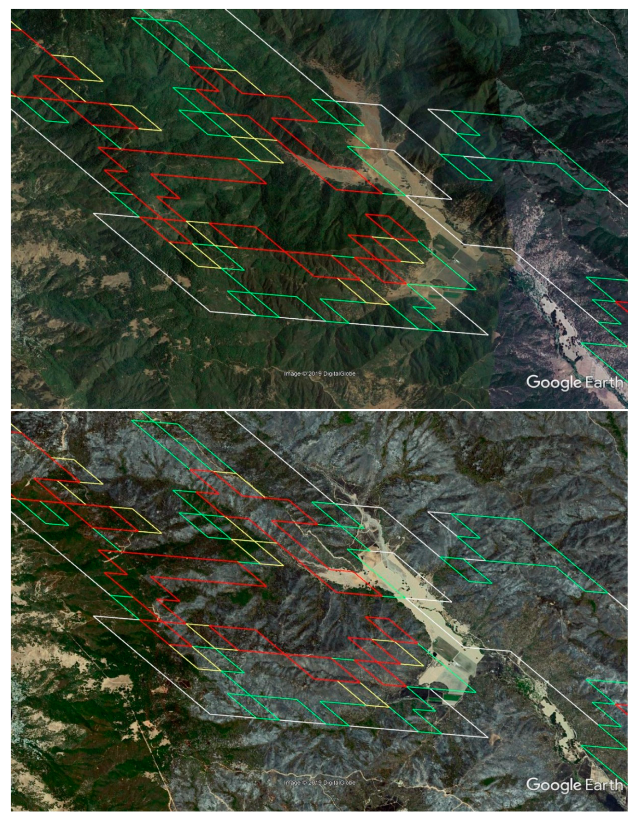
Figure 4.
Proof of concept results over the Ranch fire centered on 39.100141°, W-122.717262° on 2 July 2018 before (top) the fire and 8 August 2018 after (bottom) the fire. Overlaid are the active fire detections on 4 August 2018, DOY 216. Colored outlines mark the 500 m high (red), moderate (yellow), low (green) and poor (white) probabilities of containing active fires. It is evident that the high probability 500 m pixels show extensive fire damage while the low to poor probability pixels are less affected. Low and poor probability pixels are distinctly visible over the dry riverbed. Base imagery from Google Earth™.

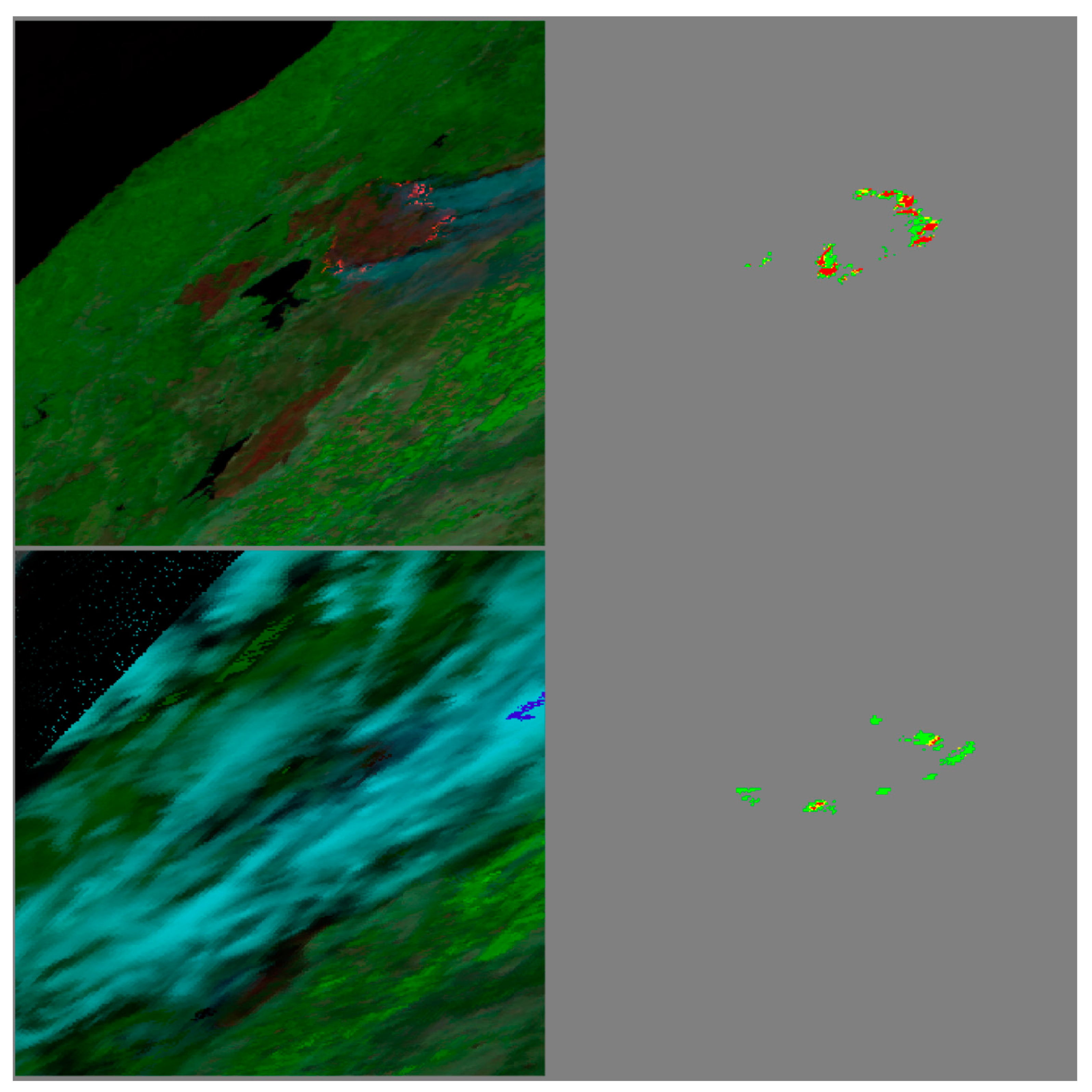
Figure 5.
Proof of concept results for the Ranch fire 150 km × 150 km subset centered on N 39.03, W 122.78 on 4 August 2018, DOY 216 (top) and 5 August 2018, DOY 217 (bottom). Left images are false color composite using red (2.13 μm), green (0.85 μm), and blue (0.64 μm) reflectance bands. Under clear skies (top), the downscaling algorithm assigns the high and moderate probabilities (red and yellow respectively) to pixels with obvious flaming fronts (right image). The algorithm is less useful if the active fires are obscured by smoke and or clouds and most pixels are assigned with a homogenous low probability (green) (bottom left image).


Table 1.
Algorithm assessment test site location, MODIS image day of year (DOY), MODIS tile, MODIS product, and accuracy assessment imagery.
Table 1.
Algorithm assessment test site location, MODIS image day of year (DOY), MODIS tile, MODIS product, and accuracy assessment imagery.
| Test Sites | Year/DOY(s) | Modis Tiles | Products (Resolution) | Accuracy Assessment Imagery (Resolution) |
|---|---|---|---|---|
| Gas flares (Iraq) | 2019/032 | H22V05 | MOD14A1 (1 km) MOD09GA (500 m) | Google Earth™ (<1–30 m) |
| Wildfire in African savanna | 2001/229 | H19V10 | MOD14A1 (1 km) MOD09GA (500 m) | ASTER (15–30 m) |
| Wildfire in US (Ranch fire) | 2018/216,217 | H08V05 | MYD14A2 (1 km) MYD09GA (500 m) | Google Earth™ (<1–30 m) |
Table 2.
Algorithm assessment results. Column 2 shows the number of 500 m candidate pixels that were encompassed by the 1 km detection. Columns 36—show the number of 500 m pixels assigned probability class High, Moderate, Low, and Poor using the downscaling algorithm. Values in parenthesis indicate the number pixels with an evident flare (active and inactive flare stack).
| # Pixels | |||||
|---|---|---|---|---|---|
| Cluster ID | Candidate 500 m | High Prob. | Moderate. Prob. | Low Prob. | Poor Prob. |
| 1 | 8 | 1 (1) | 2 (0) | 5 (0) | 0 (0) |
| 2 | 24 | 6 (3) | 1 (0) | 14 (0) | 3 (0) |
| 3 | 12 | 2 (2) | 0 (0) | 5 (0) | 5 (0) |
| 4 | 20 | 6 (3) | 0 (0) | 9 (0) | 5 (0) |
| 6 | 12 | 3 (2) | 0 (0) | 2 (0) | 6 (0) |
| 7 | 16 | 2 (0) | 2 (1) | 9 (0) | 3 (0) |
| 8 | 4 | 2 (2) | 0 (0) | 1 (0) | 1 (0) |
| 9 | 8 | 3 (0) | 0 (0) | 3 (1) | 2 (0) |
| 11 | 20 | 2 (1) | 2 (0) | 4 (0) | 12 (0) |
| 12 | 4 | 2 (1) | 0 (0) | 2 (0) | 0 (0) |
| 13 | 16 | 2 (0) | 1 (0) | 11 (1) | 2 (0) |
| 14 | 24 | 4 (2) | 0 (0) | 12 (0) | 3 (0) |
| 15 | 16 | 3 (2) | 13 (0) | 0 (0) | 0 (0) |
| 16 | 8 | 2 (1) | 3 (1) | 2 (0) | 0 (0) |
| 17 | 16 | 2 (2) | 0 (0) | 7 (0) | 6 (0) |
| 18 | 16 | 2 (1) | 2 (1) | 5 (0) | 7 (0) |
| 19 | 4 | 3 (1) | 0 (0) | 1 (1) | 0 (0) |
© 2019 by the authors. Licensee MDPI, Basel, Switzerland. This article is an open access article distributed under the terms and conditions of the Creative Commons Attribution (CC BY) license (http://creativecommons.org/licenses/by/4.0/).
Share and Cite
MDPI and ACS Style
Kumar, S.S.; Picotte, J.J.; Peterson, B. Prototype Downscaling Algorithm for MODIS Satellite 1 km Daytime Active Fire Detections. Fire 2019, 2, 29. https://0-doi-org.brum.beds.ac.uk/10.3390/fire2020029
AMA Style
Kumar SS, Picotte JJ, Peterson B. Prototype Downscaling Algorithm for MODIS Satellite 1 km Daytime Active Fire Detections. Fire. 2019; 2(2):29. https://0-doi-org.brum.beds.ac.uk/10.3390/fire2020029
Chicago/Turabian StyleKumar, Sanath Sathyachandran, Joshua J. Picotte, and Birgit Peterson. 2019. "Prototype Downscaling Algorithm for MODIS Satellite 1 km Daytime Active Fire Detections" Fire 2, no. 2: 29. https://0-doi-org.brum.beds.ac.uk/10.3390/fire2020029