
Wind in a Natural and Artificial Wildland Fire Fuel Bed
by
 , ,
, ,
Yana Bebieva
1,2,* ,
,
Kevin Speer
1,3, 
Liam White
3,
Robert Smith
4,
Gabrielle Mayans
4 and
Bryan Quaife
1,3 1
Geophysical Fluid Dynamics Institute, Florida State University, Tallahassee, FL 32306, USA
2
School of Earth and Atmospheric Sciences, Georgia Institute of Technology, Atlanta, GA 30332, USA
3
Department of Scientific Computing, Florida State University, Tallahassee, FL 32306, USA
4
FAMU-FSU College of Engineering, Tallahassee, FL 32310, USA
*
Author to whom correspondence should be addressed.
Fire 2021, 4(2), 30; https://0-doi-org.brum.beds.ac.uk/10.3390/fire4020030
Submission received: 29 April 2021
/
Revised: 6 June 2021
/
Accepted: 7 June 2021
/
Published: 9 June 2021
(This article belongs to the Special Issue Wind Fire Interaction and Fire Whirl)
Abstract
:Fuel beds represent the layer of fuel that typically supports continuous combustion and wildland fire spread. We examine how wind propagates through and above loose and packed pine needle beds and artificial 3D-printed fuel beds in a wind tunnel. Vertical profiles of horizontal velocities are measured for three artificial fuel beds with prescribed porosities and two types of fuel beds made with long-leaf pine needles. The dependence of the mean velocity within the fuel bed with respect to the ambient velocity is linked to the porosity. Experimental results show significant structure to the vertical profile of mean flow within the bed, and suggest that small-scale sweeps and ejections play a role in this system redistributing momentum similar to larger-scale canopy flows.
1. Introduction
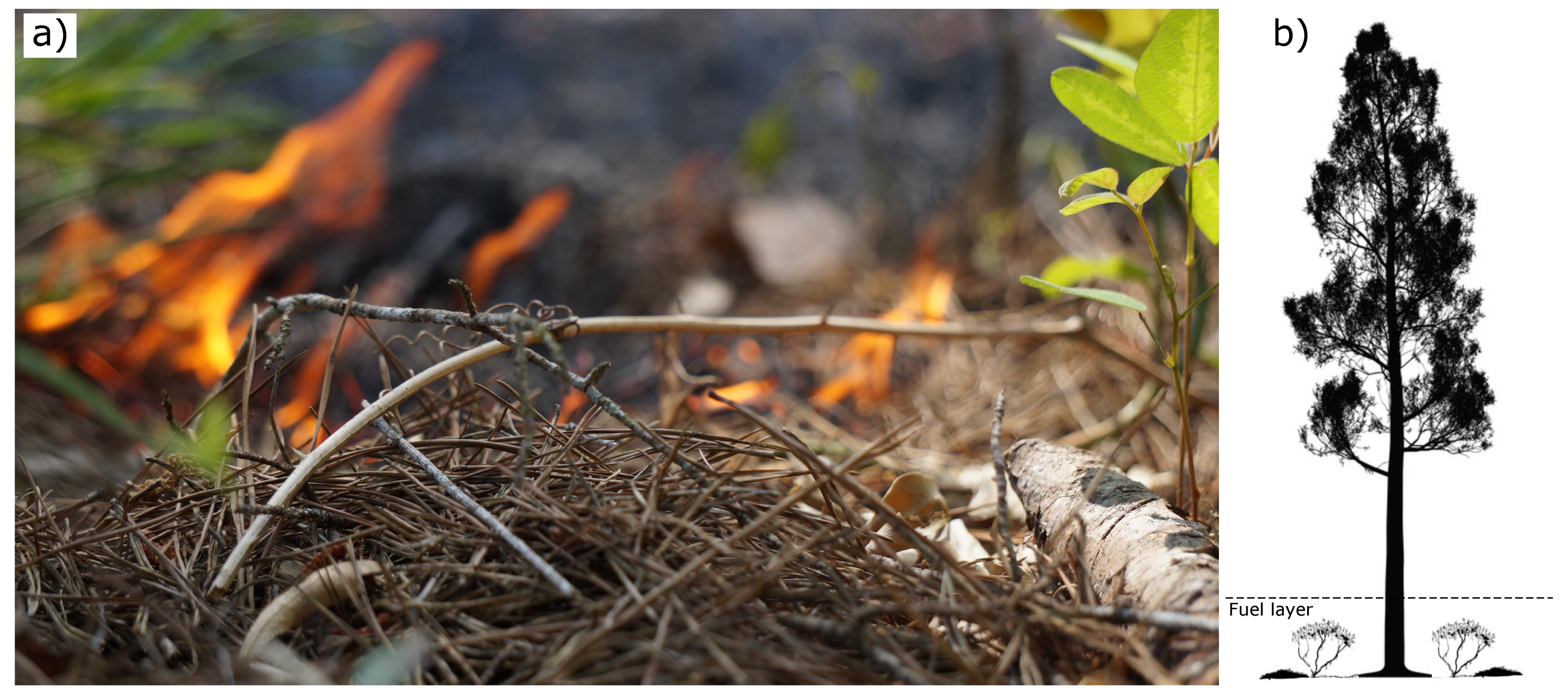
The degree of fire behavior predictability in numerical models strongly depends on the correct representation of the surface wind and its interaction with surface or ground fuels. Here, we examine the vertical structure of horizontal wind within the lowest part of the atmospheric boundary layer—the fuel layer, which typically consists of pine needles, branches, and leaves [1] (Figure 1). The presence of vegetation modifies the conventional logarithmic model of the flow within the boundary layer; in this region, the flow patterns are controlled by the structure of the vegetation including vegetation type (i.e., whether it is composed of pine straws, leaves, or litter), density, and shape of the fuel layer [2,3]. The eddies generated close to the rough boundaries influence the total vertical exchange of mass, momentum, and heat. Moreover, for combustion, oxygen inflow is critical and is also controlled by the eddy dynamics. These dynamics depend, in turn, on the vertical structure of the mean velocity field within and above the surface layer.
Much progress representing the vertical structure of mean wind flow and momentum flux in canopies analytically and numerically has been achieved [4,5,6]. Analytical models such as Massman et al. [4] can be used to estimate operationally relevant wind parameters for empirical fire spread models. Physical models with complex combustion or simplified reaction terms require the wind characteristics within the fuel bed. For example, the role of convective heat transport in fire spread has been investigated in a variety of porous fuel layer models [7,8,9,10,11,12]. In such models, the ambient wind within the fuel layer has no vertical spatial variation and is proportional to the ambient wind velocity above the fuel layer. A key parameter is thus an attenuation factor that multiplies the external ambient wind speed , lowering it to values expected in the fuel bed . This factor is typically of order 0.1 [7] but varies across diverse fuels and porosities. The aim of this paper is to establish the detailed structure and the basic characteristics of the flow within and above a representative fuel layer in a controlled experimental laboratory setting. One outcome of our study is values of for several examples of natural and artificial fuel beds.
Turbulence is generated both above and within the fuel bed or canopy. Wind tunnel experiments with artificial forests were conducted in the past [13,14] and showed a turbulent kinetic energy peak in the higher frequency range for heights within the canopy, which presumably reflect the abundance of vortices shed by model canopy elements. However, it was later suggested that the dominant turbulence within the canopy is a result of the shearing of the mean flow aloft and not that generated by the canopy elements themselves [15]. The characteristic horizontal length scale of the flow around the canopy top was shown to be at least of the canopy height [16]. In a sequence of papers [17,18], Finnigan further confirmed that momentum in the canopy is transferred by eddies whose spacial scale is larger than the canopy characteristic scales. Quadrant-hole analyses [19] of the canopy flow showed that the momentum transfer within and at the top of the canopy is mainly manifested through sweeps and ejections [17,18,20,21]. Intermittent sweeps, or strong gusts with and (where u is the longitudinal velocity component, w is vertical velocity component, and primes denote the fluctuations from the mean) were shown to dominate within and just above the canopy, whereas ejections dominate in the internal sublayer, much farther above the canopy top. It is interesting to note that the intermittent momentum transport by sweep–ejection cycles can account for approximately 50% of the flux. However, the flux also depends on the flow conditions and canopy type [22]. More recent spectral analyses of time series of the flow within the canopy showed that the eddy size did not change with height (for an overview, see [23]).
We explore a different morphology of the canopy compared to those experiments involving artificial trees [13,14,24]. Instead, we focus on a configuration that resembles a surface fuel layer, that is, porous media, rather than stand-alone elements. The velocity above the fuel layer in the field depends on the type of canopy. In our experiments, we take the background wind tunnel velocity as background velocity above the fuel layer, whether it is an exponential profile as in many canopy types or a logarithmic profile in the absence of vegetation.
The structure of the paper is as follows. In Section 2, we describe the experimental setup. In Section 3, we provide an overview of the theoretical developments on the flow structure in the porous media, within different types of canopy and the layer above it. Experimental results are discussed in the context of theory in Section 4. The conclusions and discussion are given in Section 5.
2. Materials and Methods
2.1. Experimental Setup
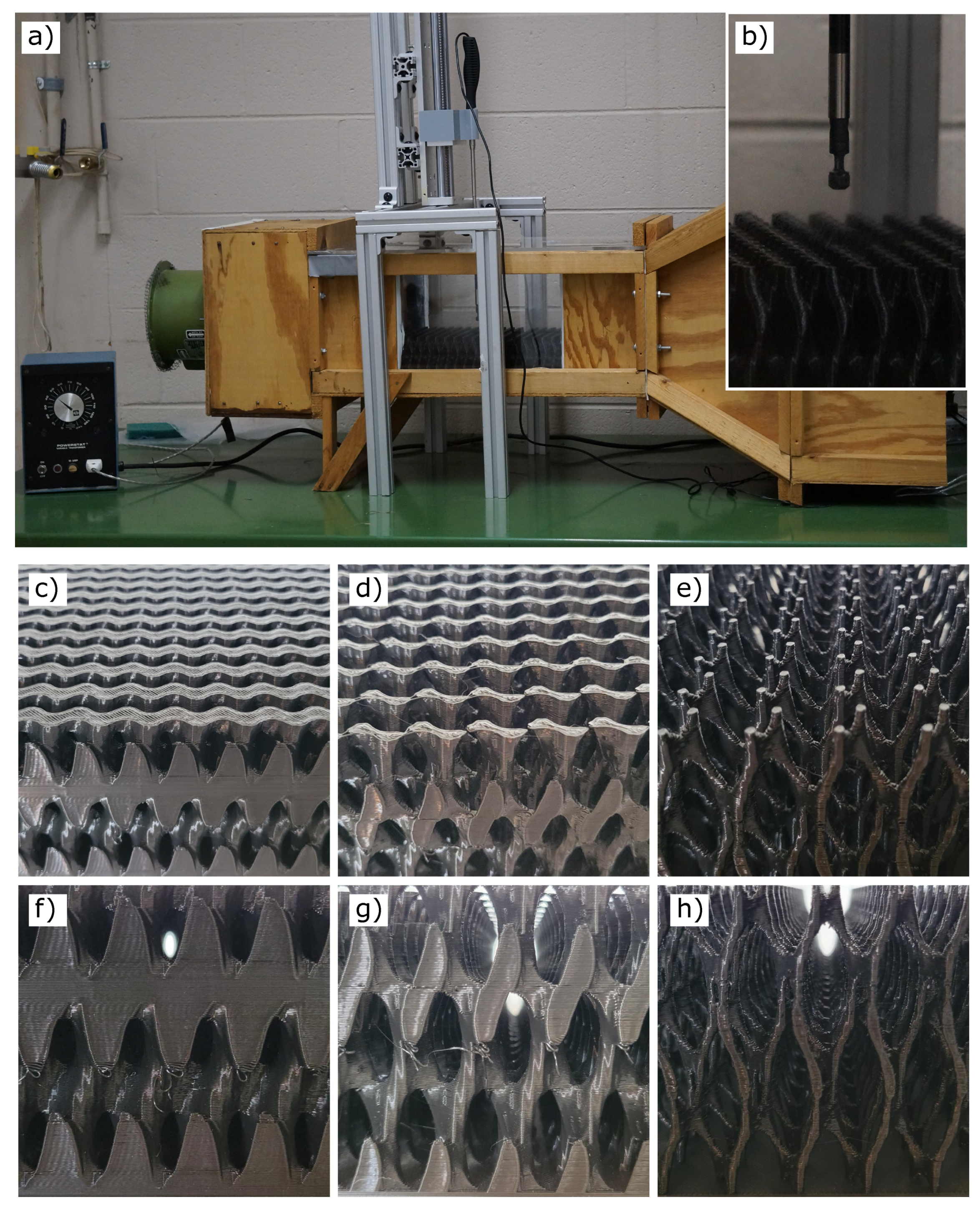
Experiments were conducted in the low-speed wind tunnel located at the Geophysical Fluid Dynamics Institute at Florida State University. It is an Eiffel-type single-pass wind tunnel, with test section visual access from the sides: top view and side view (Figure 2a,b). The dimensions of the test section of the wind tunnel are 0.53 m × 0.25 m × 0.25 m. The wind tunnel has a lid with two openings, located at 17.5 and 31 cm from the left edge of the test section, through which the velocity measurements were taken. The openings were made in the top lid to provide access at various along-stream locations. Measurements at 17.5 and 31 cm distance from the front edge were selected to provide adequate spacing of at least one fuel bed thickness distance, from the front adjustment region and rear edge region affecting the flow around these corners of the bed. When an opening is not in use, it is covered to eliminate the flow through the opening. The free-stream velocities of the wind tunnel with the empty test section were m/s and m/s, corresponding to a Reynolds number of and , based on the length of the test section and viscosity of air.
Flow velocity measurements within the tunnel were taken with a manual hot wire anemometer PCE-423 with a telescopic probe that was mounted on a linear guide (Figure 2b). The anemometer is designed for low air speeds and it enables fast and precise measurements within a range of 0.1–25 m/s, with 0.01 m/s resolution. The accuracy of the velocity measurements is 5% and the sampling rate is 1 Hz. The velocity measurements were taken every 5 mm from the bottom within the fuel layer up to the height of the maximum velocity above the fuel layer. Air leakage around the sensing element was avoided by careful placement of fuel and the sensing element. At each height, the measurements were taken for 2 min. We used two types of models for the fuel beds: 3D-printed fuel bed models and pine needle fuel bed models. Both are discussed below.
2.2. 3D-Printed Fuel Bed Models
To replicate porous fuel beds, physical models were designed and 3D printed. The physical model was based on a gyroid lattice that can be approximated by the trigonometric equation
The parameters , , and are related to the gyroid cell size in the x, y, and z dimensions, respectively, and C is a constant isovalue related to the physical model’s target porosity [25]. By choosing a gyroid, the model is triply-periodic, resembles a porous fuel bed structure, and desired porosities can be obtained by choosing appropriate values of , , , and C. To ensure successful printing, physical models with overhangs greater than 45 degrees require support structures which would increase the material costs of printing and change the porosity. To avoid such overhangs, the parameters were chosen so that no layer-to-layer overhangs were greater than 45 degrees. We used and , thus compressing the model cell density in the x and y dimensions relative to the z dimension. Each mathematical model was generated following (1) using the Minimal Surface Lattice Generator [26] with the parameters in Table 1.
The isovalues were determined through an iterative process of successively entering new isovalues until the target porosity was acquired. Once generated, the mathematical models were exported as stereolithography (STL) files and printed on a LulzBot TAZ Workhorse 3D printer using Polyactic Acid (PLA) 3D printing filament (Figure 2c–h). The physical dimensions of each model are 9.5 in × 9.5 in × 3 in (corresponding to 24.1 cm × 24.1 cm × 7.6 cm).
Physics-based fire models, such as FARSITE [27], BEHAVE [28], and FIRETEC [29], require different fuel parameters including the surface-to-volume ratio. For each of the 3D-printed models, we calculated the surface-to-volume ratio. We used two different techniques to validate the calculations, and all results agree to at least four digits. The first technique used a well-tested CAD software. The second technique relied on surface integrals that are decomposed into a sum over individual triangle elements of the mesh. The surface area of individual triangles was determined by dividing the cross-product of the vectors that span the triangle by two. The total volume is reduced to a surface integral using the divergence theorem, and the necessary surface integrals are computed analytically. This calculation was performed using the built-in function get_mass_properties in the numpy-stl library.
The computed surface-to-volume ratios (Table 2) of each model are consistent with those reported for various fuel types. In the case of the 50% model, our value of 106 ft is consistent with a 10 h fuel type (109 ft) reported by Albini [30] and implemented by Burgan and Rothermel [28]. For the 95% model, 501 ft is consistent with a 1 h fuel type (500 ft) reported by Prichard et al. [31]. The 80% model falls in the range between 1 and 10 h fuels with a surface-to-volume ratio of 206 ft.
2.3. Pine Needle Fuel Bed Models
Pine needles were used to replicate fuel beds found in nature. Two different packing densities were used to model different situations occurring within nature. The lightly packed model represents an undisturbed pine needle fuel bed that would build up from falling pine needles; the mass of the pine needles is 75 g, occupying the same volume as the 3D printed model. The packed model of pine needles represents a fuel bed that has been packed down by external forces; the mass of the pine needles in this case is 150 g, occupying the same volume as the 3D-printed model. Both models have the same dimensions as the 3D-printed models and were secured to the base of the wind tunnel using polyvinylpyrrolidone solution.
3. Theoretical Overview
In this section, we discuss previous results regarding the flow interaction at the interface of the permeable beds (see the full overview in Wood et al. [32] and Venditti et al. [33]). Fundamental processes occurring at such boundaries influence mass and momentum exchange between the bed and the free flow above.
In the flow over vegetation, there are at least three regimes of turbulent mixing resulting from canopy wake: an (emergent zone), the Kelvin–Helmholtz instability (mixing-layer zone), and the bed shear (log-law zone) representing the classical boundary-layer problem. The existence of such regimes was first suggested by Poggi et al. [34] and Nezu and Sanjou [35] based on laboratory experiments. These regimes were postulated not to overlap in space as the physical balances describing each regime are principally different, and the production mechanism of vortices in one zone would inhibit the generation of vortices from the other zone.
More recent studies use Large-Eddy Simulations (LES) [36] to show that near the canopy top (i.e., in the mixing-layer zone), the emerging spanwise-oriented coherent structures resemble hairpin vortices [2,37]. As the flow evolves the vortices dominate the vertical transport in and out of the canopy. Furthermore, the hairpin vortices may break down and generate a wide range of vorticity scales. A more recent LES numerical study by Monti et al. [38] examined the role of a different type of vortices—those generated through the Kelvin–Helmholtz (KH) instability at the top of the canopy, which are then modified by the outer flow. The authors showed that these KH vortices redistribute the local momentum within and outside the canopy layer.
These developments emphasize the need to explore and test parameterizations for turbulent fluxes in the surface boundary layer. Translating the results into quantities useful for wildland fire modeling is a challenge not only due to the complexity of the turbulent flow in and above canopies and fuel beds but also the vast range of models for fire spread, with different requirements [39,40]. Turbulence and other unresolved heat flux components have been described and incorporated into models for fire spread in fuel layers; their representation is particularly clear in reaction-diffusion models [10,12]. But even high-resolution LES meteorological and combustion models nevertheless require subgrid-scale parameterizations of small-scale turbulent fluxes of heat, momentum, and oxygen within the fuel bed which can take the form of a turbulent diffusion coefficient [5,41].
Building on this notion of a turbulent diffusion coefficient in the fuel bed (Bebieva et al. [42]) and to explore the structure of the lateral diffusivity in the fuel layer, we follow the simplest model
where L is the length scale of the dominant flow structure and is streamwise velocity fluctuations. In light of the recent findings that the flow within the canopy is controlled by the large-scale eddies originating aloft, we use the plane mixing layer theory [43] to estimate the large-scale eddy size. A plane mixing layer forms when two regions of parallel flow with different magnitudes of horizontal velocities are brought in contact. The vertical profile of the resultant flow exhibits an inflection point that is observed in the canopy flows [37,44]. The thickness of the plane mixing layer is and we will use this scale for L. In this formulation, is the velocity difference across the transition from the fuel bed to the layer above, and is the maximum vertical gradient of horizontal velocity measured across the transition zone.
We compare the estimates of the lateral diffusivity following (2) with those derived from Taylor’s frozen turbulence hypothesis [45]. According to this hypothesis turbulent eddies are advected by the mean flow, and
where T is the integral timescale computed from the velocity auto-correlation and angle-brackets denote averaging over time T.
4. Experimental Results
We present experimental results focusing on the properties of mean streamwise velocity profiles and fluctuations as a function of different fuel beds (i.e., material and porosities). The vertical profile of the streamwise velocity at the bottom boundary layer of the wind tunnel is well-described by the conventional log-layer model, e.g., see an overview in [46]
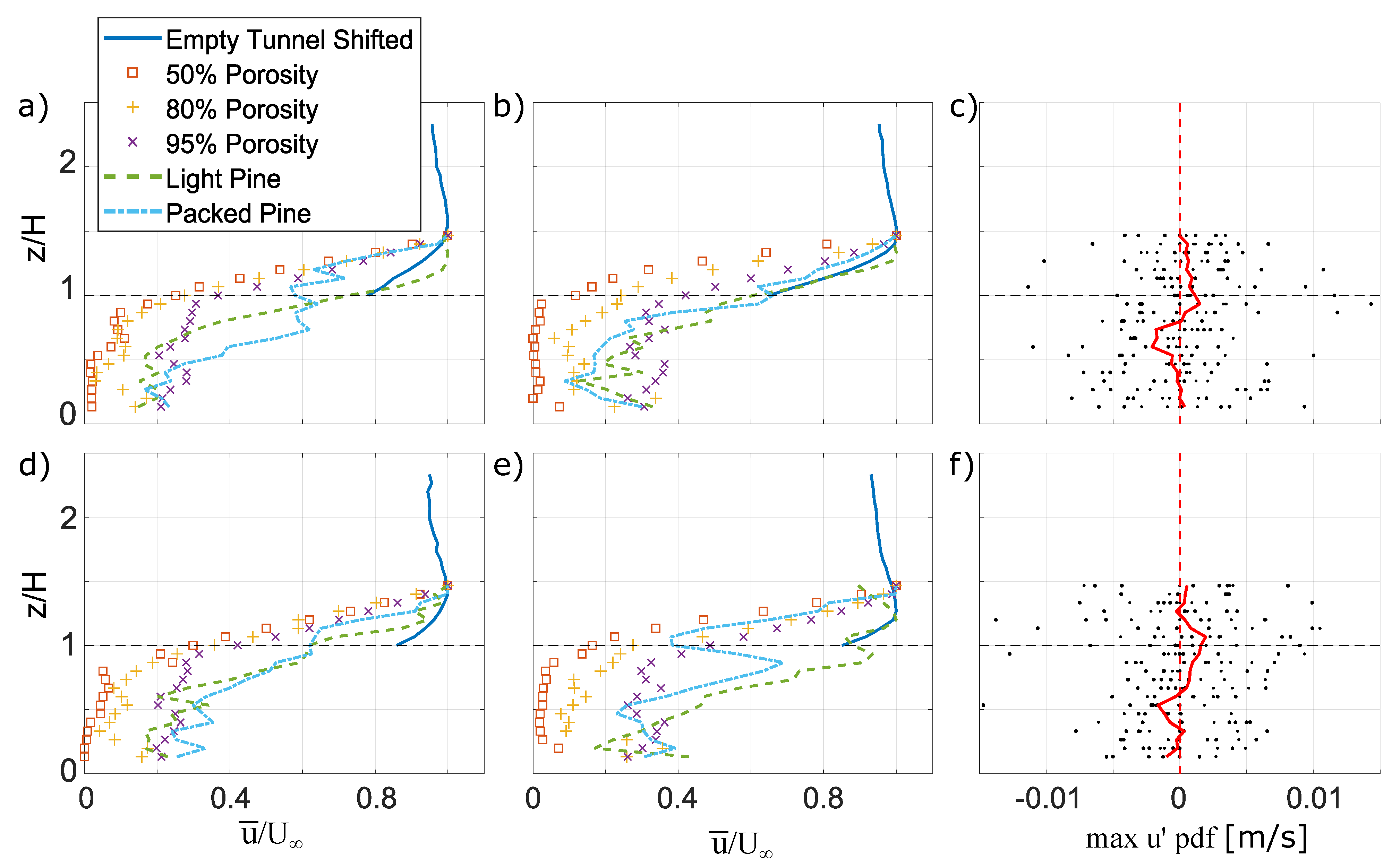
where is the friction velocity, is the Von Karman constant, is the roughness parameter, and z is height above the ground surface. Given that we only measure the streamwise velocity component, the friction velocity cannot be estimated and and are taken as parameters. Using a standard error minimization technique, mm and m/s are found to be the best fit parameters for the observations taken in the empty wind tunnel with two different background velocities. To compare the empty wind tunnel boundary layer properties with the boundary layer above the fuel models, the “empty wind tunnel” profiles (Figure 3a,b,d,e; blue solid lines) are shifted up by the thickness of the fuel models.
The vertical profiles of horizontal velocity within the fuel layer and aloft resemble those obtained within different types of canopy. Many studies report an inverse “S”-shaped profile [47,48,49], with the details of the profiles depending on vegetation morphology and plant densities [50]. Here, we do not resolve the friction layer immediately above the floor (). However, a relatively homogeneous velocity structure within the fuel layer and an inflection point above it are clearly observed (Figure 3a,b,d,e). The profiles taken within the pine needles display additional structure, for example the peaks near (Figure 3e). Such a structure may be related to fuel element wake effects but is beyond the scope of the current work.
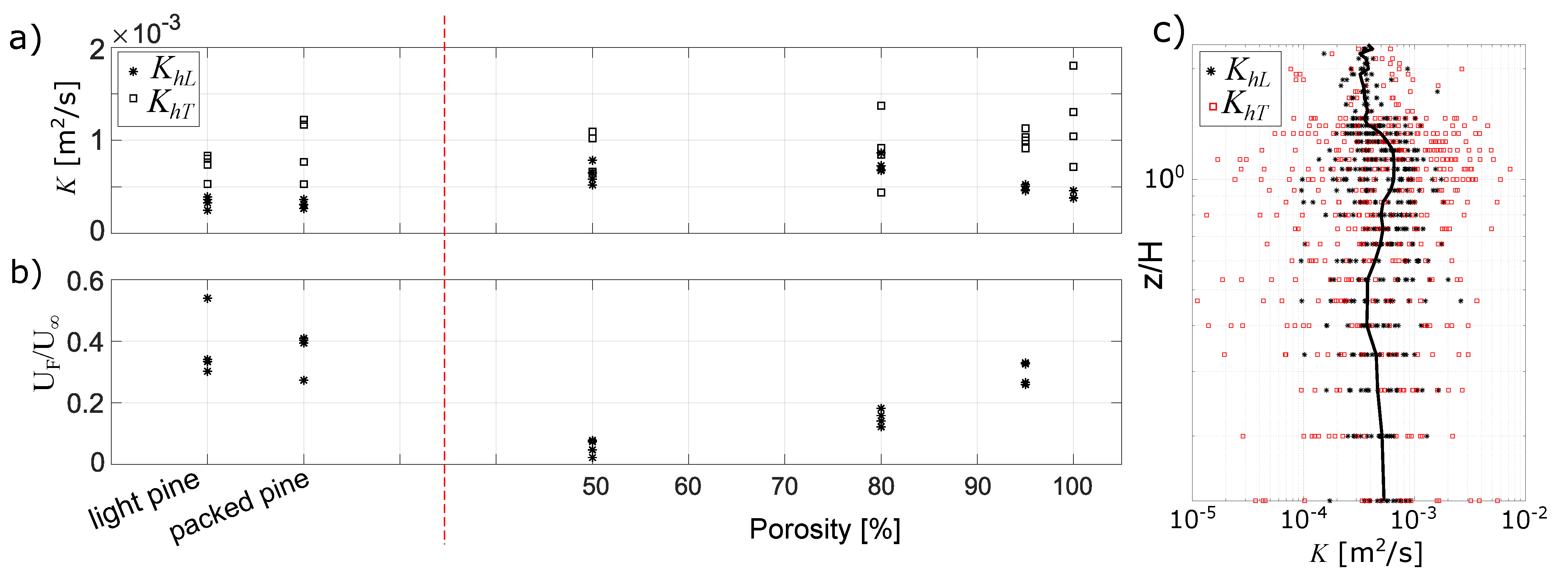
The thickness of the plane mixing layer for most of the profiles (Figure 3) is approximately cm. Lateral diffusivity computed following (2) and (3) shows slightly elevated turbulent levels at the canopy top, with an essentially uniform profile within the fuel ranging around ms (Figure 4c). There is no significant dependence of diffusivity on porosity (Figure 4a). On the other hand, the ratio increases with porosity (Figure 4b) with for the 50% model and for the 95% model, which appears consistent with previous estimates [7]. Note that within the pine beds is approximately 0.4, similar to 95% porosity.
5. Discussion
The present study describes the flow structure within fuel beds of several different porosities. In terms of a simple fuel layer, we showed that the average velocity within the fuel layer can be approximated by multiplying the mean velocity aloft by the scaling parameter , which depends on porosity. However, there is substantial vertical structure within the bed, and the fuel beds composed of the pine needles show a more complicated vertical structure of the along-stream velocity that should be addressed in greater detail in further studies.
In their numerical model, Bebieva et al. [42] interpreted the heat diffusion term as representing fluctuations in wind that move the hot gases back and forth within the fuel matrix, igniting unburnt fuel due to the eddying motion of the wind. In this model, the diffusion coefficient represents the turbulent diffusion of heat in the porous fuel layer. In our series of experiments, we do not have measurements of the vertical component of the velocity to fully characterize the momentum transport within the fuel layer. However, we can draw some conclusions by examining the streamwise velocity fluctuations .
These observations give us some insight on the dominant mixing processes within and above the fuel layer. Figure 3c,f show corresponding to the maximum PDF of at each height. Near and above the fuel layer the fluctuations are positive suggesting sweeps. Within the fuel layer , suggesting that ejections might dominate the vertical transport in this region. This finding agrees with recent LES results [38], showing the momentum control by ejection events within a stem-type canopy (their Figure 10) in a confined channel. Moreover, earlier work by Blois et al. [51] found that near-wall flow structures of permeable boundaries are best characterized by intense sweep events, as opposed to impermeable boundary flow structures which are best characterized by high and low-speed streaks and intense ejection events. A more comprehensive study involving Particle Image Velocimetry (PIV) technique is underway to investigate this conjecture in fuel bed conditions.
Our study suggests that the low-momentum flow within the fuel layer is being transferred upward and the high momentum flow above the fuel layer is being transferred downward across the top of the fuel bed (), similar to turbulent canopy flows. Diffusion is similar across a range of fuel bed characteristics. In the presence of fire, the evolving morphology of the fuel layer over time would certainly contribute to the dynamics. This has important implications for the supply of oxygen into the fuel layer and fuel combustion, as well as for heat transfer within the bed.
Author Contributions
Conceptualization, K.S. and B.Q.; Data curation, R.S. and G.M.; Formal analysis, Y.B., R.S. and G.M.; Funding acquisition, K.S. and B.Q.; Investigation, Y.B.; Methodology, K.S. and B.Q.; Project administration, B.Q.; Resources, L.W. and B.Q.; Software, L.W.; Visualization, Y.B., R.S. and G.M.; Writing—original draft, Y.B., K.S., L.W. and B.Q. All authors have read and agreed to the published version of the manuscript.
Funding
This research was supported by the U.S. Department of Defense, Strategic Environmental Research and Development Program under Award Number RC20-1298; and by the Geophysical Fluid Dynamics Institute, Florida State University.
Acknowledgments
We would like to thank Eric Adams and his team at the Florida State University Innovation Hub Fablab who helped develop and manufacture the 3D-printed models. We thank three anonymous reviewers for their constructive and thoughtful reviews.
Conflicts of Interest
The authors declare no conflict of interest.
References
- Varner, J.M.; Kane, J.M.; Kreye, J.K.; Engber, E. The flammability of forest and woodland litter: A synthesis. Curr. For. Rep. 2015, 1, 91–99. [Google Scholar] [CrossRef]
- Finnigan, J. Turbulence in plant canopies. Annu. Rev. Fluid Mech. 2000, 32, 519–571. [Google Scholar] [CrossRef]
- Chung, D.; Hutchins, N.; Schultz, M.P.; Flack, K.A. Predicting the Drag of Rough Surfaces. Annu. Rev. Fluid Mech. 2021, 53, 439–471. [Google Scholar] [CrossRef]
- Massman, W.J.; Forthofer, J.; Finney, M.A. An improved canopy wind model for predicting wind adjustment factors and wildland fire behavior. Can. J. For. Res. 2017, 47, 594–603. [Google Scholar] [CrossRef] [Green Version]
- Mueller, E.; Mell, W.; Simeoni, A. Large eddy simulation of forest canopy flow for wildland fire modeling. Can. J. For. Res. 2014, 44, 1534–1544. [Google Scholar] [CrossRef]
- Pimont, F.; Dupuy, J.L.; Linn, R.R.; Dupont, S. Impacts of tree canopy structure on wind flows and fire propagation simulated with FIRETEC. Ann. For. Sci. 2011, 68, 523–530. [Google Scholar] [CrossRef] [Green Version]
- Simeoni, A.; Santoni, P.A.; Larini, M.; Balbi, J.H. Proposal for theoretical improvement of semi-physical forest fire spread models thanks to a multiphase approach: Application to a fire spread model across a fuel bed. Combust. Sci. Technol. 2001, 162, 59–83. [Google Scholar] [CrossRef] [Green Version]
- Morandini, F.; Simeoni, A.; Santoni, P.A.; Balbi, J.H. A model for the spread of fire across a fuel bed incorporating the effects of wind and slope. Combust. Sci. Technol. 2005, 177, 1381–1418. [Google Scholar] [CrossRef]
- Koo, E.; Pagni, P.; Stephens, S.; Huff, J.; Woycheese, J.; Weise, D. A simple physical model for forest fire spread rate. Fire Saf. Sci. 2005, 8, 851–862. [Google Scholar] [CrossRef]
- Mandel, J.; Bennethum, L.S.; Beezley, J.D.; Coen, J.L.; Douglas, C.C.; Kim, M.; Vodacek, A. A wildland fire model with data assimilation. Math. Comput. Simul. 2008, 79, 584–606. [Google Scholar] [CrossRef] [Green Version]
- Babak, P.; Bourlioux, A.; Hillen, T. The effect of wind on the propagation of an idealized forest fire. SIAM J. Appl. Math. 2009, 70, 1364–1388. [Google Scholar] [CrossRef] [Green Version]
- Simeoni, A.; Salinesi, P.; Morandini, F. Physical modelling of forest fire spreading through heterogeneous fuel beds. Int. J. Wildland Fire 2011, 20, 625–632. [Google Scholar] [CrossRef] [Green Version]
- Meroney, R.N. Characteristics of wind and turbulence in and above model forests. J. Appl. Meteorol. 1968, 7, 780–788. [Google Scholar] [CrossRef] [Green Version]
- Sadeh, W.; Cermak, J.; Kawatani, T. Flow over high roughness elements. Bound.-Layer Meteorol. 1971, 1, 321–344. [Google Scholar] [CrossRef]
- Baines, G. Turbulence in a wheat crop. Agric. Meteorol. 1972, 10, 93–105. [Google Scholar] [CrossRef]
- Inoue, E. On the Turbulent Structure of Airflow within crop canopies. J. Meteorol. Soc. Jpn. Ser. II 1963, 41, 317–326. [Google Scholar] [CrossRef] [Green Version]
- Finnigan, J. Turbulence in waving wheat. Bound.-Layer Meteorol. 1979, 16, 181–211. [Google Scholar]
- Finnigan, J. Turbulence in waving wheat. II. Structure of momentum transfer. Bound.-Layer Meteorol. 1979, 16, 213–236. [Google Scholar]
- Wallace, J.M. Quadrant analysis in turbulence research: History and evolution. Annu. Rev. Fluid Mech. 2016, 48, 131–158. [Google Scholar] [CrossRef]
- Shaw, R.H.; Tavangar, J.; Ward, D.P. Structure of the Reynolds stress in a canopy layer. J. Appl. Meteorol. Climatol. 1983, 22, 1922–1931. [Google Scholar] [CrossRef] [Green Version]
- Raupach, M.; Coppin, P.; Legg, B. Experiments on scalar dispersion within a model plant canopy part I: The turbulence structure. Bound.-Layer Meteorol. 1986, 35, 21–52. [Google Scholar] [CrossRef]
- Brunet, Y. Turbulent flow in plant canopies: Historical perspective and overview. Bound.-Layer Meteorol. 2020, 177, 315–364. [Google Scholar] [CrossRef]
- Kaimal, J.C.; Finnigan, J.J. Atmospheric Boundary Layer Flows: Their Structure and Measurement; Oxford University Press: Oxford, UK, 1994. [Google Scholar]
- Bai, K.; Meneveau, C.; Katz, J. Experimental study of spectral energy fluxes in turbulence generated by a fractal, tree-like object. Phys. Fluids 2013, 25, 110810. [Google Scholar] [CrossRef]
- Liu, F.; Mao, Z.; Zhang, P.; Zhang, D.Z.; Jiang, J.; Ma, Z. Functionally graded porous scaffolds in multiple patterns: New design method, physical and mechanical properties. Mater. Des. 2018, 160, 849–860. [Google Scholar] [CrossRef]
- Al-Ketan, O.; Abu Al-Rub, R.K. MSLattice: A free software for generating uniform and graded lattices based on triply periodic minimal surfaces. Mater. Des. Process. Commun. 2020, e205. [Google Scholar] [CrossRef]
- Finney, M.A. FARSITE, Fire Area Simulator—Model Development and Evaluation; US Department of Agriculture, Forest Service, Rocky Mountain Research Station: Ogden, UT, USA, 1998; Volume 3.
- Burgan, R.E.; Rothermel, R.C. BEHAVE: Fire Behavior Prediction and Fuel Modeling System, Fuel Subsystem; US Department of Agriculture, Forest Service, Intermountain Forest and Range Forest and Range Experiment Station: Ogden, UT, USA, 1984; Volume 167.
- Linn, R.R. A Transport Model for Prediction of Wildfire Behavior; Technical Report; Los Alamos National Lab.: Los Alamos, NM, USA, 1997. [Google Scholar]
- Albini, F.A. Estimating Wildfire Behavior and Effects; Department of Agriculture, Forest Service, Intermountain Forest and Range Experiment Station: Ogden, UT, USA, 1976; Volume 30.
- Prichard, S.J.; Sandberg, D.V.; Ottmar, R.D.; Eberhardt, E.; Andreu, A.; Eagle, P.; Swedin, K. Fuel Characteristic Classification System Version 3.0: Technical Documentation; General Technical Report PNW-GTR-887; US Department of Agriculture, Forest Service, Pacific Northwest Research Station: Portland, OR, USA, 2013; 79p. [Google Scholar]
- Wood, B.D.; He, X.; Apte, S.V. Modeling turbulent flows in porous media. Annu. Rev. Fluid Mech. 2020, 52, 171–203. [Google Scholar] [CrossRef] [Green Version]
- Venditti, J.G.; Best, J.L.; Church, M.; Hardy, R.J. Coherent Flow Structures at Earth’s Surface; John Wiley & Sons: Hoboken, NJ, USA, 2013. [Google Scholar]
- Poggi, D.; Porporato, A.; Ridolfi, L.; Albertson, J.; Katul, G. The effect of vegetation density on canopy sub-layer turbulence. Bound. Layer Meteorol. 2004, 111, 565–587. [Google Scholar] [CrossRef]
- Nezu, I.; Sanjou, M. Turburence structure and coherent motion in vegetated canopy open-channel flows. J. Hydro-Environ. Res. 2008, 2, 62–90. [Google Scholar] [CrossRef]
- Bailey, B.N.; Stoll, R. The creation and evolution of coherent structures in plant canopy flows and their role in turbulent transport. J. Fluid Mech. 2016, 789, 425–460. [Google Scholar] [CrossRef] [Green Version]
- Raupach, M.; Finnigan, J.; Brunet, Y. Coherent eddies and turbulence in vegetation canopies: The mixing-layer analogy. In Boundary-Layer Meteorology 25th Anniversary Volume, 1970–1995; Springer: Berlin/Heidelberg, Germany, 1996; pp. 351–382. [Google Scholar]
- Monti, A.; Omidyeganeh, M.; Pinelli, A. Large-eddy simulation of an open-channel flow bounded by a semi-dense rigid filamentous canopy: Scaling and flow structure. Phys. Fluids 2019, 31, 065108. [Google Scholar] [CrossRef]
- Noonan-Wright, E.K.; Opperman, T.S.; Finney, M.A.; Zimmerman, G.T.; Seli, R.C.; Elenz, L.M.; Calkin, D.E.; Fiedler, J.R. Developing the US wildland fire decision support system. J. Combust. 2011, 2011, 168473. [Google Scholar] [CrossRef]
- Coen, J. Some requirements for simulating wildland fire behavior using insight from coupled weather—Wildland fire models. Fire 2018, 1, 6. [Google Scholar] [CrossRef] [Green Version]
- Linn, R.R.; Cunningham, P. Numerical simulations of grass fires using a coupled atmosphere–fire model: Basic fire behavior and dependence on wind speed. J. Geophys. Res. Atmos. 2005, 110. [Google Scholar] [CrossRef]
- Bebieva, Y.; Oliveto, J.; Quaife, B.; Skowronski, N.S.; Heilman, W.E.; Speer, K. Role of horizontal eddy diffusivity within the canopy on fire spread. Atmosphere 2020, 11, 672. [Google Scholar] [CrossRef]
- Wygnanski, I.; Fiedler, H.E. The two-dimensional mixing region. J. Fluid Mech. 1970, 41, 327–361. [Google Scholar] [CrossRef]
- Raupach, M.; Finnigan, J.; Brunet, Y. Coherent eddies in vegetation canopies. In Proceedings of the 4th Australasian Conference on Heat and Mass Transfer, Christchurch, New Zealand, 9–12 May 1989. [Google Scholar]
- Taylor, G.I. Diffusion by continuous movements. Proc. Lond. Math. Soc. 1922, 2, 196–212. [Google Scholar] [CrossRef]
- Lee, X. Fundamentals of Boundary-Layer Meteorology; Springer: Berlin/Heidelberg, Germany, 2018. [Google Scholar]
- Fons, W.L. Influence of forest cover on wind velocity. J. For. 1940, 38, 481–486. [Google Scholar]
- Bergen, J.D. Vertical profiles of windspeed in a pine stand. For. Sci. 1971, 17, 314–321. [Google Scholar]
- Oliver, H. Wind profiles in and above a forest canopy. Q. J. R. Meteorol. Soc. 1971, 97, 548–553. [Google Scholar] [CrossRef]
- Miri, A.; Dragovich, D.; Dong, Z. Wind flow and sediment flux profiles for vegetated surfaces in a wind tunnel and field-scale windbreak. Catena 2021, 196, 104836. [Google Scholar] [CrossRef]
- Blois, G.; Best, J.L.; Christensen, K.T.; Hardy, R.J.; Smith, G.H.S. Coherent flow structures in the pore spaces of permeable beds underlying a unidirectional turbulent boundary layer: A review and some new experimental results. Coherent Flow Struct. Earth’s Surf. 2013, 43–62. [Google Scholar] [CrossRef]
Figure 1.
(a) A typical mixed fuel composition of the fuel layer in a pine forest, with prescribed fire in the background. (b) A schematic showing the vegetated fuel layer with respect to a typical pine tree.
Figure 1.
(a) A typical mixed fuel composition of the fuel layer in a pine forest, with prescribed fire in the background. (b) A schematic showing the vegetated fuel layer with respect to a typical pine tree.

Figure 2.
(a) Wind tunnel setup and (b) a close up view of the test section and the sensor. (c–h) The 3D-printed models observed from the top (the top row) and side (the bottom row). (c,f) At 50% porosity; (d,g) 80% porosity; (e,h) 95% porosity.
Figure 2.
(a) Wind tunnel setup and (b) a close up view of the test section and the sensor. (c–h) The 3D-printed models observed from the top (the top row) and side (the bottom row). (c,f) At 50% porosity; (d,g) 80% porosity; (e,h) 95% porosity.

Figure 3.
Mean streamwise velocity measured within the test section of the wind tunnel at (a) 17.5 and (b) 31 cm from the leftmost position (see in Figure 2a). The mean wind profile in the empty wind tunnel (solid blue line) is shifted upward by the thickness of the fuel models (0.075 m). (c) Streamwise velocity fluctuations () corresponding to the maximum probability density function (PDF) of at each height from all measurements within the fuel layer (black dots); the red line indicates the mean values of the PDF of at each height. The background maximum velocity in the empty wind tunnel is m/s. (d–f) are the same as in (a–c) but for m/s.

Figure 4.
(a) Averaged lateral eddy diffusivity within the fuel layer () computed following (2) and (3). All data are shown (4 data points for each porosity, two background speeds, and two locations within the wind tunnel; some points overlap). Porosity of 100% corresponds to the empty wind tunnel. (b) The ratio of the averaged streamwise velocity within the fuel layer () and the background velocity . (c) Vertical profile of the lateral diffusivity estimated for all observations following (2) (black stars) and (3) (red squares).


Table 1.
The parameters used to construct models of varying porosities using the Minimal Surface Lattice Generator. X, Y, and Z are the number of lattice cells in each dimension. The mesh density refers to the number of points per cell. The isovalue C controls the porosity of the model.
Table 1.
The parameters used to construct models of varying porosities using the Minimal Surface Lattice Generator. X, Y, and Z are the number of lattice cells in each dimension. The mesh density refers to the number of points per cell. The isovalue C controls the porosity of the model.
| Relative Porosity (%) | X | Y | Z | Mesh Density | Isovalue C |
|---|---|---|---|---|---|
| 50 | 9.5 | 9.5 | 3.0 | 100 | −0.0007 |
| 80 | 9.5 | 9.5 | 3.0 | 100 | 0.8426 |
| 95 | 9.5 | 9.5 | 3.0 | 100 | 1.21855 |
Table 2.
Surface-to-volume ratio of the 3D-printed models.
| Relative Porosity (%) | Surface-to-Volume Ratio (ft) | Surface-to-Volume Ratio (m) |
|---|---|---|
| 50 | 106 | 347 |
| 80 | 206 | 677 |
| 95 | 501 | 1643 |
Publisher’s Note: MDPI stays neutral with regard to jurisdictional claims in published maps and institutional affiliations. |
© 2021 by the authors. Licensee MDPI, Basel, Switzerland. This article is an open access article distributed under the terms and conditions of the Creative Commons Attribution (CC BY) license (https://creativecommons.org/licenses/by/4.0/).
Share and Cite
MDPI and ACS Style
Bebieva, Y.; Speer, K.; White, L.; Smith, R.; Mayans, G.; Quaife, B. Wind in a Natural and Artificial Wildland Fire Fuel Bed. Fire 2021, 4, 30. https://0-doi-org.brum.beds.ac.uk/10.3390/fire4020030
AMA Style
Bebieva Y, Speer K, White L, Smith R, Mayans G, Quaife B. Wind in a Natural and Artificial Wildland Fire Fuel Bed. Fire. 2021; 4(2):30. https://0-doi-org.brum.beds.ac.uk/10.3390/fire4020030
Chicago/Turabian StyleBebieva, Yana, Kevin Speer, Liam White, Robert Smith, Gabrielle Mayans, and Bryan Quaife. 2021. "Wind in a Natural and Artificial Wildland Fire Fuel Bed" Fire 4, no. 2: 30. https://0-doi-org.brum.beds.ac.uk/10.3390/fire4020030