
Assessing Potential Safety Zone Suitability Using a New Online Mapping Tool


1
Department of Geography, University of Utah, Salt Lake City, UT 84112, USA
2
USDA Forest Service, Rocky Mountain Research Station, Fort Collins, CO 80526, USA
3
USDA Forest Service, Rocky Mountain Research Station, Missoula, MT 59801, USA
*
Author to whom correspondence should be addressed.
Fire 2022, 5(1), 5; https://0-doi-org.brum.beds.ac.uk/10.3390/fire5010005
Submission received: 12 November 2021
/
Revised: 26 December 2021
/
Accepted: 5 January 2022
/
Published: 7 January 2022
(This article belongs to the Special Issue Wildfire Hazard and Risk Assessment)
Abstract
:Safety zones (SZs) are critical tools that can be used by wildland firefighters to avoid injury or fatality when engaging a fire. Effective SZs provide safe separation distance (SSD) from surrounding flames, ensuring that a fire’s heat cannot cause burn injury to firefighters within the SZ. Evaluating SSD on the ground can be challenging, and underestimating SSD can be fatal. We introduce a new online tool for mapping SSD based on vegetation height, terrain slope, wind speed, and burning condition: the Safe Separation Distance Evaluator (SSDE). It allows users to draw a potential SZ polygon and estimate SSD and the extent to which that SZ polygon may be suitable, given the local landscape, weather, and fire conditions. We begin by describing the algorithm that underlies SSDE. Given the importance of vegetation height for assessing SSD, we then describe an analysis that compares LANDFIRE Existing Vegetation Height and a recent Global Ecosystem Dynamics Investigation (GEDI) and Landsat 8 Operational Land Imager (OLI) satellite image-driven forest height dataset to vegetation heights derived from airborne lidar data in three areas of the Western US. This analysis revealed that both LANDFIRE and GEDI/Landsat tended to underestimate vegetation heights, which translates into an underestimation of SSD. To rectify this underestimation, we performed a bias-correction procedure that adjusted vegetation heights to more closely resemble those of the lidar data. SSDE is a tool that can provide valuable safety information to wildland fire personnel who are charged with the critical responsibility of protecting the public and landscapes from increasingly intense and frequent fires in a changing climate. However, as it is based on data that possess inherent uncertainty, it is essential that all SZ polygons evaluated using SSDE are validated on the ground prior to use.
Keywords:
firefighter safety; safe separation distance; safety zones; LCES; Google Earth Engine; lidar; LANDFIRE; Landsat; GEDI1. Introduction
Wildland firefighters are tasked with a wide variety of fire management duties, many of which place them in close proximity to flames. One of the primary tasks is the removal of fuels and construction of containment lines in order to limit the potential damage to lives, property, and other critical resources [1,2,3]. Particularly when engaged in a direct attack, whereby firefighters may be working within a few meters or less of the flaming front, the potential risk for safety incidents is elevated [4]. Sudden or unexpected changes in fire behavior can have devastating effects to vulnerable fire personnel on the ground [5]. Events such as the Yarnell Hill fire in 2013, which claimed the lives of 19 firefighters and the South Canyon fire, which resulted in 14 firefighter fatalities, demonstrate the tragedy that can occur in the wildland fire profession [6,7,8]. Beyond these well-known, high-fatality events, there is an additional and significant background level of mortality that occurs among on-duty wildland firefighters [9]. The causes of death are varied, and include heart attacks, vehicular and aircraft accidents, falling trees, and smoke inhalation, to name a few. Between 1990 and 2016, there were 480 wildland firefighter fatalities, nearly one fifth (19%) of which were due to burnovers or entrapments. Burnovers are events in which flames overcome fire personnel, either on the ground or while in a vehicle, and entrapments are when firefighters become trapped by surrounding flames, unable to evacuate to safety [10]. As wildland fires increase in frequency, extent, and intensity, wildland firefighters may be put at heightened risk while working in the increasingly complex fire environment [11,12,13,14,15]. Passage of the Infrastructure Investment and Job Act in the US developing a requirement for federal agencies to “develop and adhere to recommendations for mitigation strategies for wildland firefighters to minimize exposure due to line-of-duty environmental hazards” further underscores the importance and continued policy relevance of wildland firefighter safety (see H.R. 3684 §40803(d)(5)(A)).
To avoid injury or fatality, firefighters employ a range of safety measures in anticipation of and throughout fire management operations. Safety is often considered the first priority of wildland firefighters, as evident in the 10 Standard Firefighting Orders and the 18 Watch Out Situations, colloquially referred to as the “10s and 18s” and known by all fire crews in the US [16,17]. One of the most important safety protocols is the interconnected and interdependent system of lookouts, communications, escape routes, and safety zones (LCES) [18]. First formalized by Paul Gleason in 1991, and later modified to include anchor points by Thorburn and Alexander in 2001 [19], proper implementation and continued reevaluation of LCES is essential to firefighter survival. Lookouts are members of a fire crew well-trained in the interpretation of fire behavior and weather conditions who are placed at a vantage point in the fire environment that ensures continued visual observation of the fire crew, the fire itself, and the surrounding landscape. Communications ensure that critical information is conveyed in a clear, timely, and orderly manner between various resources deployed on a fire, including ground crews, lookouts, vehicular and aerial assets, and incident command. Escape routes are pre-defined evacuation pathways that enable crews to retreat to a safety zone or other safe area. And finally, safety zones (SZs), which are the primary focus of this paper, are areas on the landscape that firefighters can retreat to in dangerous situations in order to avoid bodily harm. SZs are large, open areas with little or no flammable material contained within. They can take a variety of forms, including naturally sparsely or unvegetated areas and areas that have had fuel removed either mechanically, or through burning.
The effectiveness of SZs is defined by the extent to which they can provide safe separation distance (SSD) from surrounding or nearby flames [4,5,20,21,22]. SSD is defined as the distance one must maintain from fire to avoid burn injury, without deployment of a fire shelter [5,22]. The current operational guideline in the US for defining SSD emerged from the work of Butler and Cohen in 1998, who used radiative heat transfer modeling to determine that firefighters should maintain a distance of at least 4 times the height of the proximal flames [22]. Although this guideline has since been widely adopted [23], the research that underlies it is based solely on one heat transfer mechanism: radiation. Heat transfer by convection is also a major—sometimes dominant—force, particularly in the presence of steep slopes and high winds [24,25,26]. In the presence of such convective heat, particularly if a fire crew is upslope and/or downwind of flames, SSD will increase [5,21]. Thus, the four times flame height rule is likely insufficient in these conditions. Recent work by Butler et al. has sought to update this guideline with the inclusion of a “slope-wind factor”, which adds a multiplicative term to the SSD equation to account for the effects of convective heat transfer [5,21,26,27,28]. In addition, given that SZs should be designated prior to, rather than during, the presence of flames, the four times flame height rule requires firefighters to predict how tall the flames might eventually be, which is a challenging endeavor. Accordingly, the newly proposed guidelines assume that, in a crown fire, flame height is approximately equal to twice the vegetation height [28]. As a result, the new SSD equation is defined as:
where VH is vegetation height and Δ is the slope-wind factor. Butler recently defined these slope-wind factors seen in Table 1, based not only on slope and wind speeds, but also on the burning conditions, as dictated by fuel conditions (e.g., moisture) and weather (e.g., relative humidity) [28].
Although guidelines for use on the ground are valuable, they still require the firefighters themselves to make the calculation of SSD on the ground while engaged in other fire management activities. This requires the ability to accurately estimate vegetation height and terrain slope and anticipate wind speed and fire intensity. Moreover, even if these difficult interpretations and predictions can be made, an even more challenging endeavor is to identify an area on the ground cleared of vegetation that provides the calculated SSD in all directions. In order to reduce the subjectivity of this process and the potential for interpretation error, Campbell et al. sought to develop a robust, geospatially driven approach for identifying and assessing the suitability of SZs in advance of a fire using high-resolution airborne lidar, which provides detailed terrain and vegetation height information [20]. Their method automatically identified open areas, determined the height of surrounding trees, and calculated a score for the relative suitability of potential safety zones within the open areas based on tree height and SSD. The potential for broad applicability of their approach, however, is limited by three main factors: (1) the lack of widely available airborne lidar data, (2) the temporal relevancy of and lack of scheduled updates to available lidar data, and (3) the fact that only existing clearings could be assessed. With respect to the first limitation, at present, high-quality, publicly accessible airborne lidar data is particularly sparse in the Western US, where fires are most frequent, large, and intense. Regarding the second limitation, vegetation structure is dynamic in fire-prone environments, where SZ assessment is most important. Thus, having outdated lidar data potentially limits accurate SSD calculation. Lastly, although existing open areas may be viable SZs, firefighters often use areas that have already burned (“black” areas) or create SZs through mechanical fuel removal.
To resolve the limitations of this previous work and to improve wildland firefighter safety, we are introducing a new, interactive, web-based, open-access mapping tool for estimating SSD and evaluating potential SZ effectiveness through geospatial analysis. Instead of relying on lidar, this tool uses LANDFIRE Existing Vegetation Height data, which is both nationally available in the contiguous US and is updated every few years. Additionally, instead of only assessing SSD-driven suitability on clearings that already exist, this tool allows users to draw their own SZ polygon to evaluate the potential suitability of a SZ in any environment. Since LANDFIRE vegetation heights may not be as accurate as airborne lidar, given that it is a modeled product driven by satellite imagery, it is important to quantify the effects of differing sources of vegetation height data on SSD evaluation. Accordingly, the primary objectives of this study are to: (1) introduce and describe the algorithm that underlies a new tool for calculating SSD and analyzing SZ suitability; (2) compare SSD and potential SZ suitability using different sources of vegetation height data; (3) demonstrate an example case study of the tool in a simulated wildland firefighting situation.
2. Materials and Methods
2.1. Algorithm Description
The Safe Separation Distance Evaluator (SSDE) algorithm is built and applied in Google Earth Engine (GEE), a cloud-based platform for processing and analyzing GIS and remotely sensed data, using the JavaScript application programing interface [29]. GEE was selected for few reasons: (1) it enables the production of user-facing applications that can be widely accessed by anyone with an internet connection; (2) it hosts an immense catalog of geospatial data, including datasets necessary for the analysis of SZ suitability; (3) its cloud computing capabilities provide for rapid execution of complex geospatial functions, allowing users to quickly assess SZ suitability. Accordingly, all data processing described in this section is conducted using the GEE.
The SSDE evaluates SSD in two primary ways (Figure 1). The first is per-pixel SSD, which is a representation of how far one must be from that pixel (e.g., in meters) in order to avoid burn injury (Figure 1a). This is calculated at the individual pixel level across an entire area of interest based on the vegetation height and terrain slope within each pixel, and user-defined wind speed and burn condition classes. It provides a landscape-scale view of SSD and can be used to aid in the delineation of potential SZ polygons. However, it is perhaps more important to evaluate SSD at the level of the SZ polygon, as this can help fire personnel determine the suitability of a potential SZ. Accordingly, the second way that SSDE evaluates SSD is through the analysis of proportional SSD (pSSD) within potential SZ polygons (Figure 1b). pSSD quantifies the extent to which a potential SZ polygon provides SSD from surrounding vegetation/flames, considering the average per-pixel SSD contained within a series of segments (or clusters of contiguous pixels) around the SZ polygon. Measured in percent, a pSSD of 100% or greater for a given pixel would mean that, factoring in vegetation height surrounding the polygon, slope, wind speed, and burn condition, the pixel’s location should provide sufficient SSD, should fire personnel opt to use this location as a SZ. Conversely, a pixel with a pSSD of less than 100% would indicate that firefighters located within that pixel may risk injury from burning vegetation outside the boundary of the polygon. A detailed description of the computation of both SSD and pSSD follows.
Per-pixel SSD is calculated as follows. The algorithm relies on two primary input datasets, both of which are available on a nationwide basis in the US. The first is LANDFIRE Existing Vegetation Height, version 2.0, which is a 30 m spatial resolution raster dataset where each pixel represents the average height of the dominant vegetation within that pixel (Figure 2b) [30,31]. The second is a Shuttle Radar Topography Mission (SRTM) digital elevation model (DEM), also at 30 m spatial resolution [32]. Using the SRTM DEM, terrain slope in percent is calculated (Figure 2c). This slope raster is then converted into a slope-wind factor dataset, based on user-defined wind speed and burning condition categories (Figure 2d; Table 1). Using Equation (1), SSD is calculated from the slope-wind factor and vegetation height data, producing a spatially exhaustive representation of the distance one must maintain from each pixel in the image dataset in order to avoid injury (Figure 2e). As discussed further in Section 2.3 and Section 3.3, there is a user-selected bias correction option that is built into SSDE to account for underestimation of tree heights in the LANDFIRE data.
The per-pixel, landscape-wide layers representing SSD, vegetation height, and slope, as well as the high-resolution Google imagery base map, can be used to identify potential SZ on the landscape. In a realistic wildland fire scenario, this identification process would likely be undertaken by a GIS specialist working with an incident management team, who has specific knowledge of the current fire extent, projected changes in fire behavior, and crew assignments. However, given the open-access nature of SSDE, this process can likewise be undertaken by anyone with an interest in wildland firefighter safety. To calculate pSSD at the SZ polygon level, the user can define a potential SZ using the polygon drawing tools in SSDE, guided by the conditions both within the polygon and surrounding the polygon. The best SZs are those that contain no flammable material within, naturally or otherwise, so ideally this SZ polygon would be drawn in an area with low fuel loading, such as short or sparse grasses or litter. Alternatively, a SZ polygon could also be drawn in an area that has recently burned, or an area that would be targeted for fuel removal to create a SZ.
pSSD within a SZ is dependent upon the slope and vegetation height of the surrounding landscape. As discussed in the Introduction, heat transfer from flames generally increases with increasing vegetation height and terrain slope. Accordingly, a SZ in the midst of steep terrain and tall vegetation will require a larger SSD than a SZ in the midst of flat terrain and short vegetation. If we assume that the SZ itself contains little or no flammable material, then the primary concern for SZ evaluation is the area surrounding the SZ. Accordingly, to calculate pSSD within the SZ polygon, slope and vegetation height need to be evaluated within a “buffer” surrounding a SZ [20,33]. In an environment with short vegetation, a relatively small buffer surrounding a SZ needs to be evaluated, because flame heights will tend to be low and more distant vegetation will not affect the suitability of a SZ given its limited capacity for transferring heat over long distances (Figure 3a). Conversely, in the presence of tall trees and steep slopes, larger buffer areas are needed to account for the effects of more distant fuel and flames (Figure 3b). For example, a stand of 20 m tall forest in a low-slope environment with moderate wind speed and burning conditions would require an SSD of 320 m—that is, to maintain safety, firefighters would need to find a SZ that provides at least 320 m of separation from this stand. However, if the SZ evaluation procedure only included an analysis of vegetation within a small (e.g., 20 m) buffer around the SZ, then the potentially dangerous effects of the heat emitting from a crown fire in this stand could be missed, putting the firefighters at risk.
Accordingly, to ensure that an appropriately sized buffer area is evaluated around a potential SZ polygon, the buffer size must be defined by the highest per-pixel SSD in the surrounding area. To do this, the largest theoretically possible SSD in the US (SSDUSmax) is first calculated as follows:
where VHUSmax is the height of the tallest tree in the US (116 m) and ∆max is the maximum slope-wind factor from Table 1 (10). As a result, SSDUSmax is equal to 9280 m. While this is purely a theoretical SSD, it provides a useful initial buffer distance. The potential SZ polygon is buffered by this SSDUSmax, and then the highest SSD pixel value within the initial buffer (SSDSZmax) is then identified. This value is then used to create the final buffer around a designated SZ polygon, which will serve as the basis of SSD evaluation.
The buffer area is then used to clip out a subset of the SSD raster (Figure 4a). Given that each pixel possesses its own SSD (based on its unique combination of vegetation height and slope-wind factor), it is important to consider the variation in SSD that is found throughout the area surrounding the SZ polygon. Vegetation may be taller or slopes may be steeper on one edge of a SZ polygon as compared to the other. Accounting for this spatial variability at the pixel level would greatly increase computation time, so the SSDE algorithm applies an image segmentation function on the clipped SSD raster to generate a series of segments (i.e., clusters of similar pixels) representing areas with relatively homogeneous SSD values (Figure 4a). From each segment, Euclidean distance is calculated on a continuous basis as a 30 m spatial resolution raster where each pixel represents the distance from that segment. Each segment also has a mean SSD value, aggregated from the SSD pixel values within the segment. Accordingly, a comparison between the Euclidean distance raster and the segment’s mean SSD value should provide insight into whether pixels in the SZ polygon are within or beyond the SSD. To determine this on a relative basis, the Euclidean distance is then divided by the segment’s mean SSD, resulting in a dataset containing pixels representing pSSD, where pixel values under 1 (or 100%) represent areas that would be unsafe if the fuel within that segment were burning under crown fire conditions (Figure 4b). Values over 1 (or 100%) represent areas that would be safe, according to the SSD guideline. This process is repeated for every segment surrounding the SZ polygon, producing a series of pSSD rasters. To reduce these rasters down to a single representation of pSSD within the SZ polygon, the minimum pixel value (representing the “worst-case” pSSD for all segments surrounding the polygon) is extracted among all of the rasters (Figure 4c). This pSSD raster enables the identification of the safest area within the potential SZ polygon, defined as the location with the highest pSSD (Figure 4d). Lastly, a threshold is applied to the pSSD to distinguish between safe areas, or areas that are equal to or greater than 100% of pSSD, and unsafe areas, or areas that are less than 100% of pSSD (Figure 4d). The size of the resulting safe areas is important for wildland firefighters, as it provides a sense for how many resources (e.g., firefighters, trucks, dozers, engines) can utilize the SZ at once. It has been estimated that approximately 5 m2 (50 ft2) is recommended for each firefighter, and 28 m2 (300 ft2) for each piece of heavy equipment [33,34]. To enable users to interact with the resulting data outside of GEE, there are options for downloading all of the resulting data layers, including the SSD raster, pSSD raster, safe/unsafe raster, the SZ polygon vector feature, and the safest point vector feature.
2.2. Vegetation Height Analysis
Given that LANDFIRE Existing Vegetation Height is a modeled product based on multispectral satellite imagery, it can be assumed that there is inherent inaccuracy in its vegetation height estimates. Conversely, airborne lidar data, which result from laser pulses emitted from an airborne platform reflecting off the ground and aboveground surfaces, provide direct measurements of vegetation height. Thus, airborne lidar is considered a reliable source of data for deriving accurate and precise canopy height models in vegetated environments [35]. In fact, the models that derive the LANDFIRE Existing Vegetation Height product are trained in part using airborne lidar data, in addition to ground-level plot measurements [36]. Inaccuracy in vegetation height results in inaccuracy in SSD, and inaccuracy in SSD could have significant effects on the safety of wildland firefighters. Accordingly, to quantify these effects, we compared LANDFIRE-driven SSD to lidar-driven SSD.
Although LANDFIRE is one of the most widely used, nationwide vegetation height products in the US, particularly among wildland fire scientists, it is not the only one. A recent study by Potapov et al. introduced a new global forest height product driven by a combination of Global Ecosystem Dynamics Investigation (GEDI) data and Landsat 8 OLI imagery [37,38]. GEDI is a spaceborne lidar instrument that produces large footprint (~25 m diameter) full waveform surface elevation data. Distinct from airborne lidar, however, which produces a dense point cloud of measurements that can be used to interpolate spatially exhaustive, high-resolution height models, GEDI’s sampling design is such that large gaps exist between successive and adjacent footprints, limiting the capacity to produce spatially contiguous height models. However, Potapov et al. used GEDI data to train a model to predict forest height using Landsat imagery on a global scale. Similarly to LANDFIRE, this GEDI/Landsat hybrid product is a modeled product and, as such, possesses inherent uncertainty. In the interest of basing our algorithm on the best and most reliable vegetation height data, we also compared the GEDI/Landsat-derived SSD to airborne lidar-derived SSD.
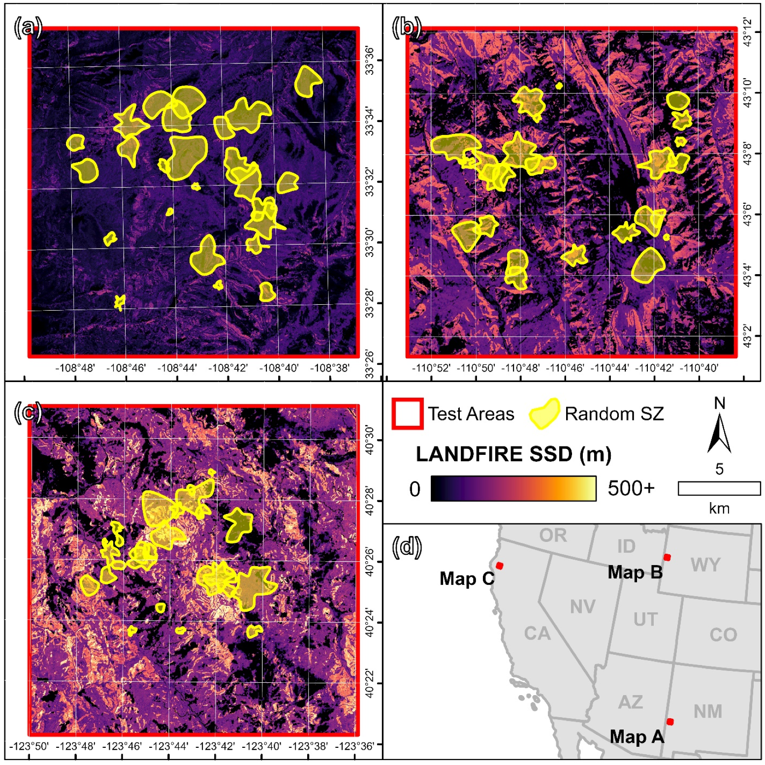
To compare LANDFIRE, GEDI/Landsat, and airborne lidar, we selected three areas in fire-prone regions of the Western US. These areas were selected to capture a range of terrain and vegetation height conditions. Importantly, each of the three areas was required to have recently collected, freely available airborne lidar data and no recent major disturbances. The 3 areas selected, each 20 × 20 km in size, are shown in Figure 5. The first area is in western New Mexico (Figure 5a), ranging in elevation from 1659 to 3032 m (mean = 2253 m), ranging in slope from 0 to 153% (mean = 26%), and is dominated by ponderosa pine forests and piñon-juniper woodlands. According to the airborne lidar data, vegetation heights range from 0 to 41 m (mean = 13 m). The second area is in western Wyoming (Figure 5b), ranging in elevation from 1741 to 3038 m (mean = 2284 m), ranging in slope from 0 to 179% (mean = 35%), and is dominated by Douglas fir and lodgepole pine forests and sagebrush shrublands. According to the airborne lidar data, vegetation heights range from 0 to 40 m (mean = 15 m). The third area is in northern California (Figure 5c), ranging in elevation from 137 to 1399 m (mean = 729 m), ranging in slope from 0 to 195% (mean = 30%), and is dominated by Douglas fir forests, black oak woodlands, and ruderal grasslands. According to the airborne lidar data, vegetation heights range from 0 to 72 m (mean = 22 m).
Airborne lidar datasets for each of these 3 areas were acquired from the USGS 3D Elevation Program (3DEP) [39]. The New Mexico data came from the USGS 3DEP dataset titled “NM_SouthCentral_2018_D19”, collected in 2018 with an average point density of 6.0 pts/m2. The Wyoming data came from the USGS 3DEP dataset titled “WY_Southwest_2020_D20”, collected in 2020 with an average point density of 7.6 pts/m2. The California data from the USGS 3DEP dataset titled “USGS_LPC_CA_NoCAL_Wildfires_B4_2018”, collected in 2018 with an average point density of 10.1 pts/m2. It should be noted that there are some temporal discrepancies between the airborne lidar data (2018–2020), LANDFIRE data (2016), and GEDI/Landsat data (2019). To avoid issues associated with major vegetation height changes that may have occurred between these time frames, these areas were selected specifically to avoid containing any fires that had occurred between 2015 and 2021. To match the training and validation data used in the development of LANDFIRE and Potapov et al.’s height products, airborne lidar canopy height models were derived at a 30 m spatial resolution using the 90th percentile of aboveground point returns within each pixel. All of the airborne lidar data processing was conducted using LAStools [40].
To assess SSD uncertainty, the algorithm described in Section 2.1 was applied to each of the three vegetation height datasets (LANDFIRE, GEDI/Landsat, and airborne lidar). However, to enable the flexibility needed for this comparative analysis, the algorithm was implemented in Python with heavy reliance on the Esri ArcPy library, rather than GEE. Given that the GEDI/Landsat product does not include vegetation heights lower than 3 m (as it is considered a “forest” height product), LANDFIRE vegetation heights were used in areas lower than 3 m in height for the GEDI/Landsat analysis. For all three datasets, the same terrain slope was used, derived from a USGS 3DEP 30 m digital elevation model. In each of the three test areas, SZ polygons were automatically generated, using a random shape generator created for this study. Briefly, it starts with a randomly located point, and then creates a shape based on a randomly defined number of equally spaced vertices that are placed at random distances from the center point. The distances are selected from a normal distribution with a mean between 100 and 1000 m and a standard deviation of 0.25 times the mean. The resulting shape is then smoothed to produce a final SZ polygon, as can be seen in Figure 5a–c. In all, 25 SZ polygons were generated for each test area (75 total). Since each polygon was evaluated independently, randomly placed polygons could overlap. For each SZ polygon, every unique combination of burning condition and wind speed was evaluated. As a result, the algorithm was run 2025 times (3 vegetation height datasets × 75 SZs × 3 burning conditions × 3 wind speeds).
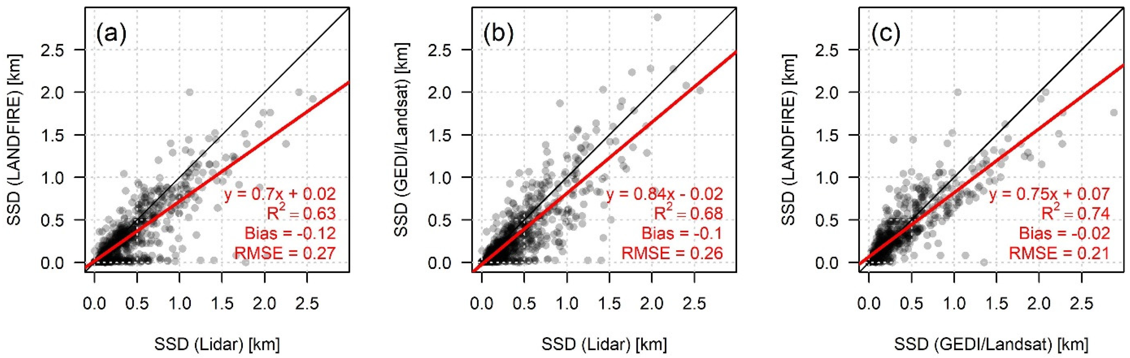
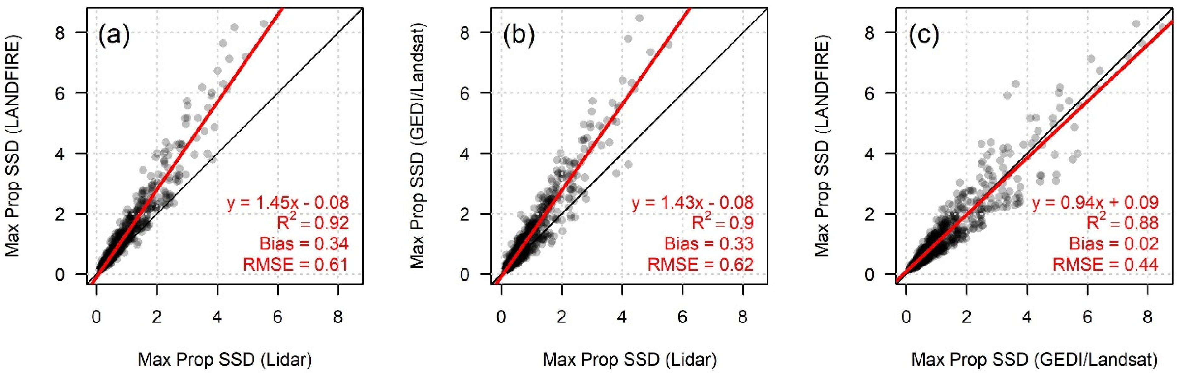
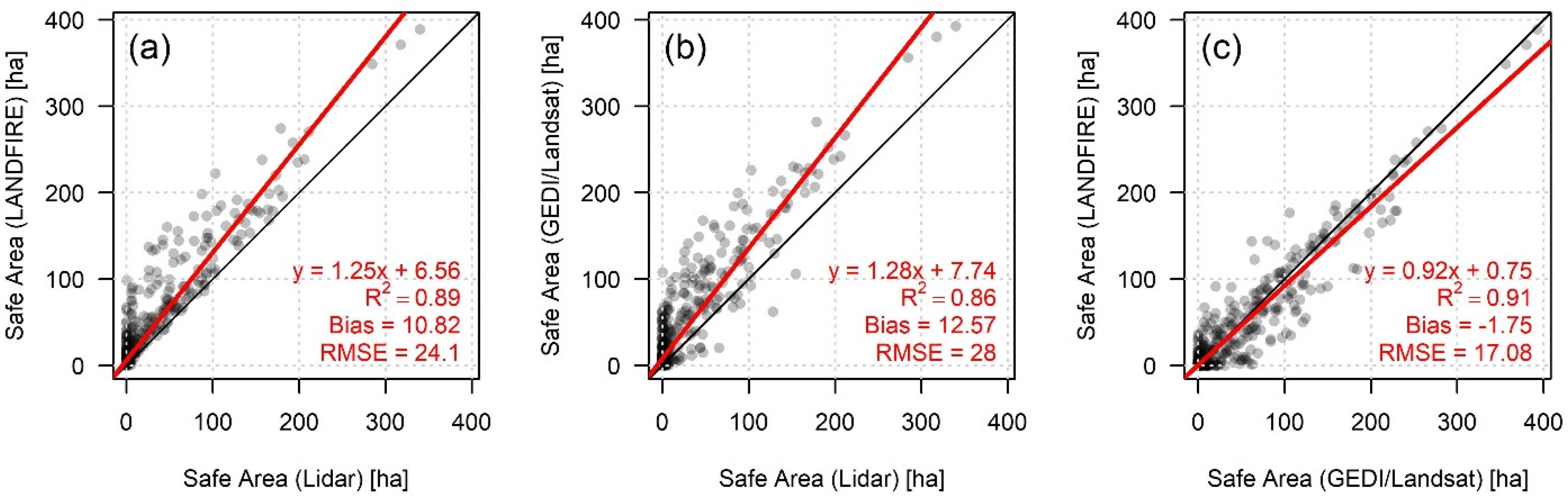
Four statistical comparisons were made between the results from the three different vegetation height datasets. The first was a per-pixel SSD comparison. For this, a set of 25 random points was generated within each combination of vegetation height dataset, burning condition, and wind speed (675 points total), and pixel values were extracted from SSD rasters. The second was the maximum pSSD found within each of the randomly generated SZ polygon for each combination of vegetation height dataset, burning condition, and wind speed. The third was the total safe area (the areas meeting or exceeding SSD) within the SZ polygon for each combination of vegetation height dataset, burning condition, and wind speed. All three of these comparisons were made using ordinary least squares regression between LANDFIRE and airborne lidar, GEDI/Landsat and airborne lidar, and LANDFIRE and GEDI/Landsat. The fourth and final statistical comparison was aimed at determining the geographic divergence between the locations identified as being the safest point within each SZ. For this, the horizontal distance between safe points was calculated between LANDFIRE and airborne lidar, GEDI/Landsat and airborne lidar, and LANDFIRE and GEDI/Landsat, from which histograms and associated descriptive statistics were derived.
2.3. LANDFIRE Bias Correction
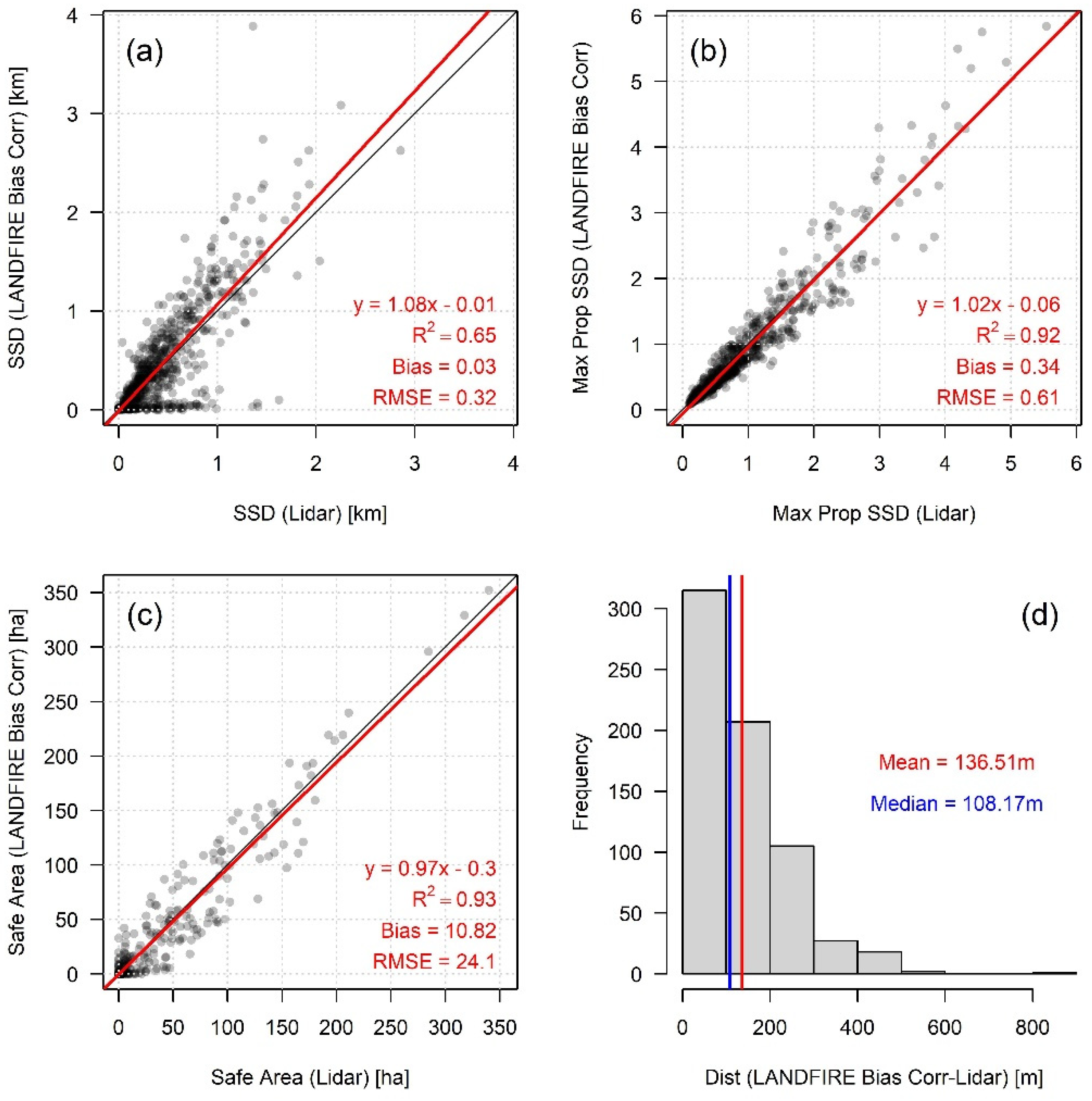
As mentioned in Section 2.1 and discussed in greater detail in the Section 3.2, the per-pixel SSD comparison revealed that, in comparison to the airborne lidar-based SSD values, the LANDFIRE and GEDI/Landsat SSD values were underestimated. To ensure that the algorithm is not overestimating the relative safety of drawn SZs, a bias correction procedure was developed. Although both LANDFIRE and GEDI/Landsat featured a similar trend in bias, the bias correction was only tested on the LANDFIRE data, given the fact that LANDFIRE was ultimately selected as the vegetation height dataset used in SSDE, the justification for which is further discussed in Section 4. To correct for underestimation in SSD, the linear regression model resulting from the per-pixel SSD comparison was used to adjust LANDFIRE SSD pixel values through a linear transformation. To test the extent to which this bias correction procedure increased the agreement between LANDFIRE- and lidar-derived SSD values and SZ suitability metrics, the same four statistical comparisons previously described were conducted: (1) per-pixel SSD linear regression; (2) within-SZ maximum pSSD linear regression; (3) within-SZ total safe area linear regression; (4) safest point distance histogram comparison. Lastly, to enable users to select between using the raw LANDFIRE data or the bias-corrected LANDFIRE data as a basis of SSD calculation, a selection option was added to SSDE.
2.4. Use Case Demonstation
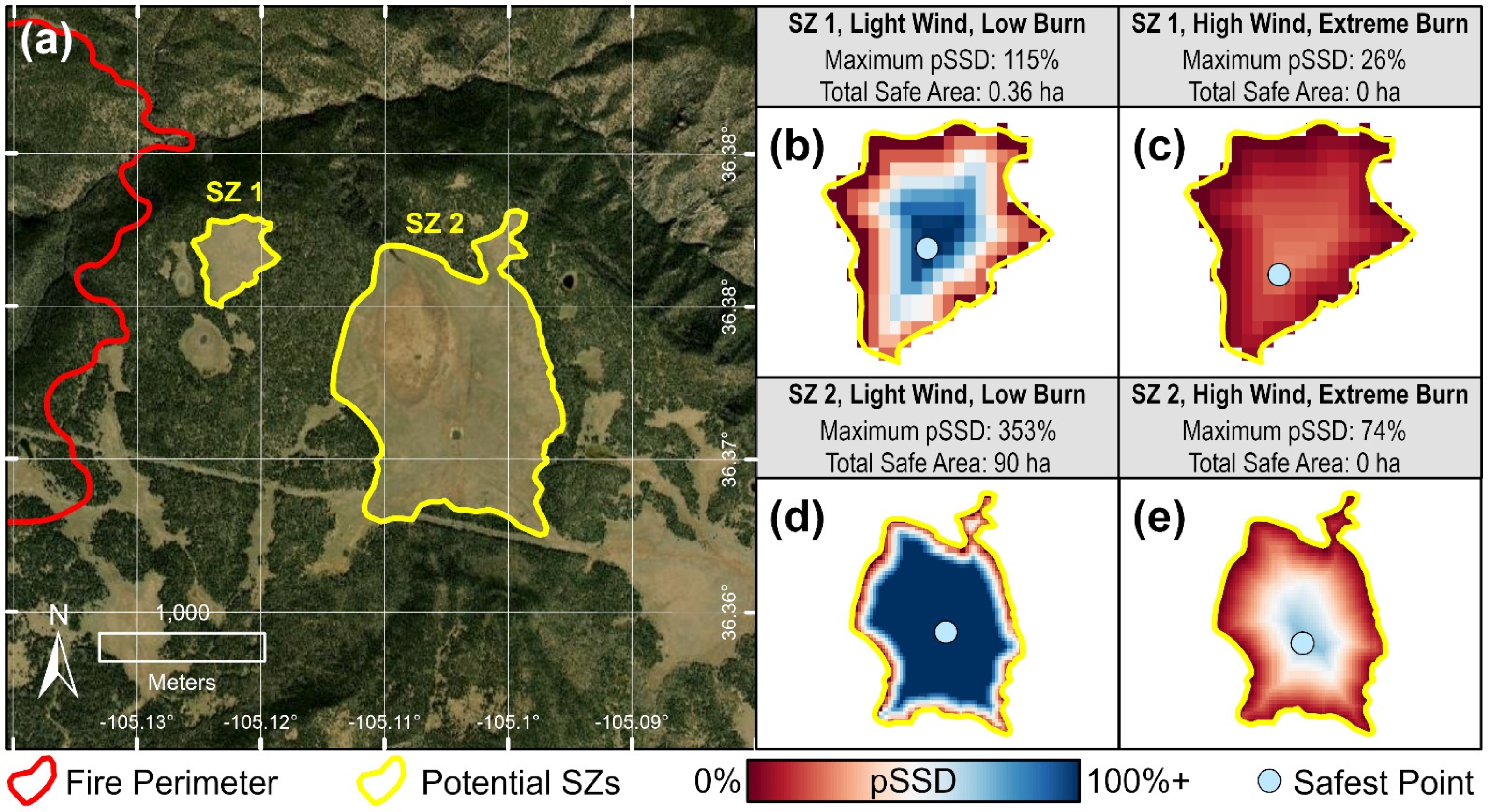
To provide an example use case for SSDE, we simulated a situation in which wildland firefighters are tasked with selecting a SZ during an active wildfire. To do this, we created a fictional fire perimeter in a ponderosa pine forest in an area of northern New Mexico that has a variety of potential SZs in the form of open grassy meadows. Two of these potential SZs are delineated and analyzed using SSDE. To test the viability of these potential SZ under different weather and fire conditions, they are each evaluated for two sets of extremes: (1) light wind and low burn condition; (2) high wind and extreme burn condition.
3. Results
3.1. GEE Application
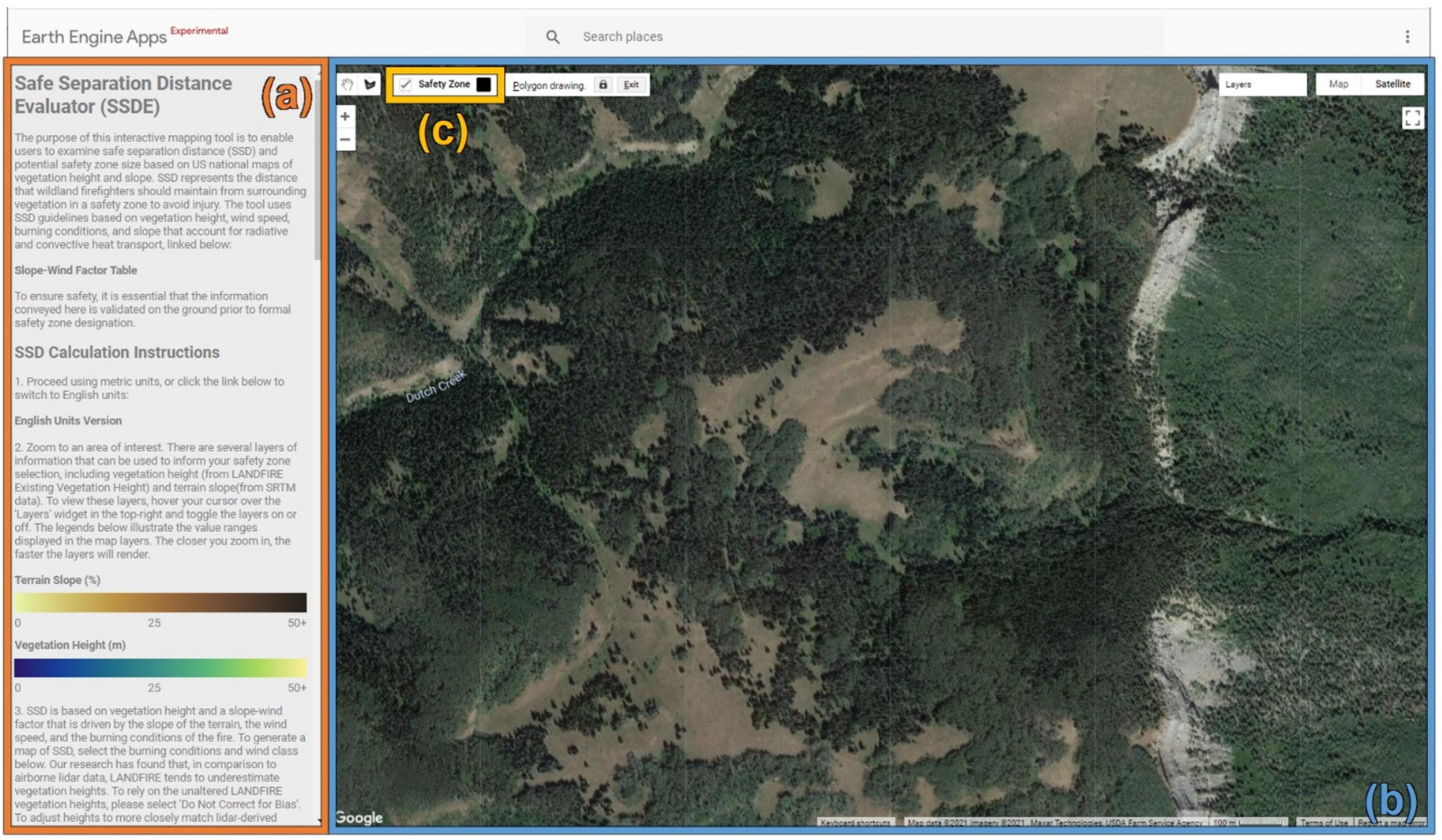
The SSDE was developed in GEE and a free, open-access, web-based application can be viewed at https://firesafetygis.users.earthengine.app/view/ssde (accessed on 3 January 2022). Screen captures of the interface can be seen in Figure 6, Figure 7 and Figure 8. Figure 6 represents the view that a user would have when zoomed to an area of interest, including an instructional panel on the left that explains how to use the tool (Figure 6a), the main map interface with a Google imagery base map (Figure 6b), and the polygon drawing tool that can be used to digitize a potential SZ polygon (Figure 6c).
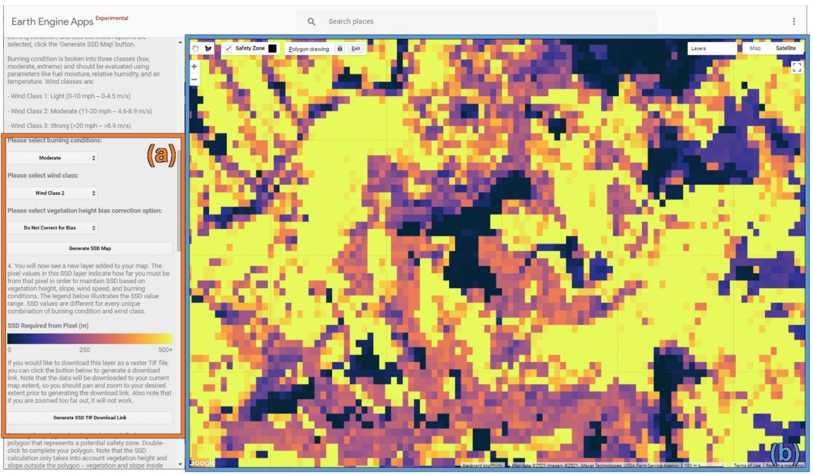
The user then has the option to select the burning condition, wind speed, and whether or not to correct for vegetation height bias (Figure 7a). Following these selections, the user generates a per-pixel SSD map (Figure 7b). The user also has the option to download the resulting raster image (Figure 7a).
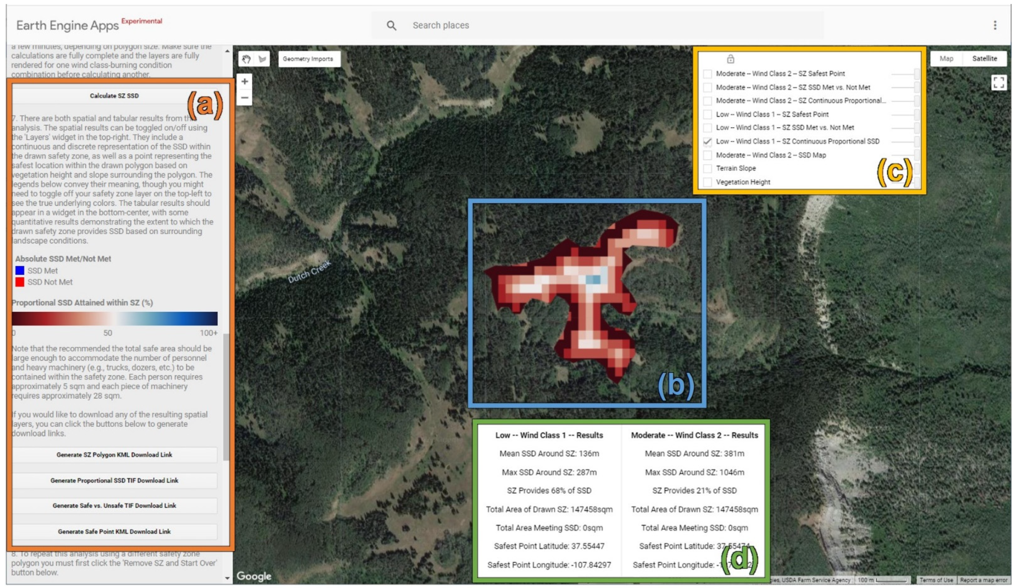
The user can then manually draw in a potential SZ polygon and evaluate a variety of suitability metrics by selecting ‘Calculate SZ SSD’ (Figure 8a). As a result, three new spatial layers will be added to the map, each within the extent of the SZ polygon, including the pSSD (Figure 8b), as well as a point feature representing the safest location and a safe (pixels greater than or equal to SSD) and unsafe (pixels less than SSD) raster. These layers can be toggled on and off in the ‘Layers’ menu (Figure 8c). The layers can also be individually downloaded (Figure 8a). Lastly, a series of tabular metrics are also computed and displayed to aid in the evaluation of SZ suitability (Figure 8d). The user can evaluate and compare multiple different wind speeds, burning conditions, and whether or not bias is corrected for.
3.2. Vegetation Height Analysis
The results of the per-pixel SSD uncertainty analysis can be seen in Figure 9. When compared to airborne lidar-derived SSD, which we assume to be the most accurate given the fact that airborne lidar vegetation heights are directly-measured rather than modeled, it becomes clear that both LANDFIRE- and GEDI/Landsat-derived SSD values, on average, are underestimated (Figure 9a,b). Since all of the other variables (slope, wind speed, burning condition) were held constant, this means LANDFIRE and GEDI/Landsat vegetation height products underestimated vegetation heights, as taller vegetation results in higher SSD. Per-pixel SSD values are still fairly strongly correlated (R2LANDFIRE-lidar = 0.63; R2GEDI/Landsat-lidar = 0.68), suggesting that the modeled products trend towards similar results as the airborne lidar-derived per-pixel SSD, but the regression slopes of less than 1 indicate that both LANDFIRE and GEDI/Landsat will underestimate per-pixel SSD, particularly on the high end. This further points towards the fact that LANDFIRE and GEDI/Landsat fail to capture the structure of very tall vegetation well, though this failure appears more pronounced in the LANDFIRE data, given the lower regression line slope. Of particular note is the presence of a number of sample points where the LANDFIRE and GEDI/Landsat per-pixel SSD values approach zero but the airborne lidar per-pixel SSD values are greater than zero. A visual assessment of the three vegetation height datasets in comparison to aerial imagery revealed that, at least in some cases, this can be attributed to the presence of standing dead vegetation such as in a post-fire environment. The airborne lidar captures this standing dead vegetation since the laser pulses interact with any aboveground objects. However, the LANDFIRE and GEDI/Landsat, both of which rely heavily on spectral data tend to suggest there is no vegetation in these areas, given the fact that the typical vegetation reflectance signal (e.g., high near infrared reflectance, low visible wavelength reflectance) is no longer present after a disturbance event. The comparison between LANDFIRE and GEDI/Landsat directly further suggests that LANDFIRE tends to underestimate vegetation heights to a greater extent than GEDI/Landsat, though they are strongly correlated (R2LANDFIRE-GEDI/Landsat = 0.74) (Figure 9c).
The results of the SZ polygon-level maximum pSSD uncertainty analysis can be seen in Figure 10. The results follow a similar trend from the per-pixel SSD comparison, which makes sense given that within-SZ pSSD is driven by the pixel-level SSD values surrounding the SZ polygon. Both LANDFIRE and GEDI/Landsat overestimate the maximum pSSD within SZ polygons as compared to airborne lidar (Figure 10a,b). This can once again be attributed to vegetation height underestimation from these modeled products as compared to airborne lidar data. In addition, there is a much greater correlation at the SZ polygon level than at the pixel level. For example, at the pixel level, LANDFIRE and lidar SSD have a coefficient of determination (R2) of 0.63, whereas at the SZ polygon level, LANDFIRE and lidar maximum pSSD have an R2 of 0.92. This is likely due in part to the segmentation procedure that aggregates adjacent pixels with similar SSD values and computes a mean, which drives the pSSD calculation, thus reducing the pixel-level noise and producing a stand-level estimate of vegetation height. This high correlation also suggests that SZ polygon size is likely the major driver of within-SZ pSSD, outweighing the effects of differing vegetation height estimates. When comparing between the 2 modeled products, LANDFIRE and GEDI/Landsat produce very similar results with a high correlation (R2LANDFIRE-GEDI/Landsat = 0.88) and a regression line slope of close to 1 (0.94) (Figure 10c). Again, even though LANDFIRE tended to produce slightly lower per-pixel SSD values due to lower vegetation height estimation (Figure 9c), when pixels are aggregated at the segment level and when those segment-level pSSD estimates are further aggregated at the SZ polygon level, subtle differences in vegetation height bear little effect on pSSD calculation.
The results of the SZ polygon-level total safe area uncertainty analysis can be seen in Figure 11. These results mirror those seen in Figure 9, which makes sense given that safe area is a direct product of the within-SZ pSSD calculation. Both LANDFIRE and GEDI/Landsat tend to overestimate total safe area within SZ polygons as compared to airborne lidar (Figure 11a,b). While such an overestimation is potentially problematic, the most acutely problematic disagreement between the modeled products and the airborne lidar is the large number of SZ polygons where lidar indicates there is 0 ha safe area and the modeled products indicate there is greater than 0 ha safe area—in some cases as much as 100 ha of safe area. However, it is important to recognize that since the safe versus unsafe classification is based on a defined pSSD threshold, a SZ polygon that reaches 99% of SSD would still be mapped as unsafe, so small differences in vegetation heights can have large effects on these results. Once again, the LANDFIRE and GEDI/Landsat safe area estimates are both highly correlated and relatively unbiased when compared to one another (Figure 11c).
The results of the safest point geographic displacement analysis can be seen in Figure 12. LANDFIRE and GEDI/Landsat result in safest points being on average between about 100 and 150 m from the lidar-derived safest point location (Figure 12a,b). Given the 30 m spatial resolution of the analysis, that means, on average, the safest points are within 3–5 pixels of one another. This suggests that the geography of the safest point is perhaps not as sensitive to the vegetation height as it is to the geometry of the SZ polygon. However, there are exceptions, given the right-skewed tail of the distributions. In a select few instances, safest points were found to be 800 m apart or more. From a firefighter safety perspective, this is a significant deviation, as the safest point is likely the target gathering point within the SZ for the crew and equipment. The LANDFIRE and GEDI/Landsat safest points are, on average, closer to one another than they each are to the airborne lidar-derived safest points (Figure 12c).
3.3. LANDFIRE Bias Correction
The results of the LANDFIRE bias correction procedure can be seen in Figure 13. The bias correction resulted in SSD and SZ suitability metrics that align more closely with those derived from airborne lidar. Specifically, in all three regression analyses, including the per-pixel SSD (Figure 13a), the within-SZ polygon maximum pSSD (Figure 13b), and the within-SZ polygon total safe area (Figure 13c), the regression slope was much closer to one than the un-corrected data. The bias correction bore little effect on the safest point location comparison, which makes sense given the fact that vegetation heights were all increased linearly, meaning the placement of the safest point would not have changed significantly (Figure 13d).
3.4. Use Case Demonstration
The results of the case study demonstration can be seen in Figure 14. The two potential SZ polygons varied in shape, size, and proximity to the fire perimeter. In a direct attack situation, a fire crew would be working in close proximity to the perimeter of the fire. Thus, having a SZ that is in close proximity to the crew is the best way to ensure that they can access the SZ quickly via a pre-planned escape route. Based on proximity alone, SZ 1 is superior to SZ 2 (Figure 14a). Indeed, provided that wind speeds were light and burn conditions were low, SZ 1 would provide sufficient SSD for the crew, providing a maximum within-SZ pSSD of 115%, and a total safe area of 0.36 ha (Figure 14b). However, under high winds and extreme burn conditions, this SZ would no longer be suitable (Figure 14c). In comparison, SZ 2 is further away, but due to its larger size, provides greater SSD, particularly under light winds and low burn conditions (Figure 14d). Even though this polygon is much larger, it still does not meet the SSD guideline under high winds and extreme burn conditions, providing a maximum within-SZ pSSD of 74% (Figure 14e). Armed with this information, however, the crew could opt to expand SZ 2 to increase its suitability through mechanical fuel removal or controlled burning.
4. Discussion
We envision the SSDE being of broad interest to the wildland fire community, from fire scientists to incident management personnel to wildland firefighters. Its open-access nature allows anyone to explore, examine, and interact with the concepts of SZs and SSD. Even if not used in an operational context, there is great value in being able to quickly and easily examine the conditions that define potential SZ suitability on a broad spatial scale. Wildland firefighters designate SZs on a daily basis as a part of their fire management duties. Built into this designation process is an inherent degree of subjectivity that can result in differences in the interpretation of SZ suitability between and among crews. By using an objective tool for SZ suitability analysis that can be broadly applied in the US, fire crews across the country can increase the consistency and reliability of the SZ evaluation process. However, given that this is a web-based platform requiring an internet connection, that also does not translate well to a mobile environment, we do not envision this as a real-time decision-making tool that firefighters could use on the ground. Instead, operational use of SSDE could be at the incident command level, for daily or more frequent evaluation of potential SZs for crews working on a fire. Given the dynamic and fast-paced nature of fire management, it is essential to be able to make rapid assessments of SZ suitability, particularly as fire conditions change. For example, cross-referencing near-real time data representing the current fire perimeter with SSDE can enable the evaluation of whether or not previously burned areas can provide SSD from nearby unburned fuel. Additionally, our SZ suitability driver analysis revealed the strong influence of wind on maximum within-SZ pSSD. This highlights the need to continually re-evaluate SZ suitability not only as the fire evolves, but as local weather conditions change as well.
There is relatively little research on the actual utilization of SZ in wildland firefighting. As discussed in the Introduction, SZ are largely designated ad hoc by firefighters, with little support from GIS and remote sensing data. As a result, there are essentially no publicly available datasets that represent SZ that were used by firefighters. If they were available, we could perform more empirically driven studies of SZ effectiveness, but as it stands, we are limited to using theoretical models to predict safety zone effectiveness based on fire physics [21,22,25,26,27]. While we do not know how many firefighters have suffered injuries or fatalities due specifically to the selection of inadequate SZ, we do know that burnovers and entrapments occur on an annual basis, and that these injuries and fatalities would be much less likely to occur if escape routes and SZ were properly employed. Every wildland fire safety incident is different from the last, so there is no systematic way to determine the extent to which a tool such as SSDE would have mitigated the incident. However, with the increased infusion of reliable geospatial data and modeling into wildland firefighter safety, we hope to minimize future incidents. In future research, it would be beneficial to compare the results of SSDE to actual SZ used by firefighters. This could be accomplished through the GPS collection of SZ in the field or perhaps through simulation of SZ selection in a virtual environment, to minimize risk to fire personnel while still gaining valuable, realistic insight into SZ selection [41,42,43].
The SSD guideline upon which SSDE is based (Equation (1), Table 1) can be quite restrictive, particularly in landscapes featuring rugged terrain and tall trees. For example, in a worst-case scenario (high winds, extreme burning conditions), trees that were 25 m tall and on slopes that were steep (>40%) would produce an SSD equal to 2 km, making SZ designation impractical, if not impossible. However, even if no SZ is found to meet guidelines, SSDE still can provide an analysis of which safety zones are closest to meeting the SSD requirement. SSDE enables evaluation of newly burned potential SZs or existing clearings that nearly meet the SSD requirement and could be enlarged through prescribed burning or mechanical fuel removal. For example, if a potential SZ polygon delineated within an existing clearing was determined through the use of SSDE to only reach a maximum pSSD of 90%, SSDE could be further used to evaluate the relative suitability of one or more potential SZ expansion options. These options could be informed by the aerial imagery, terrain, vegetation height, and SSD data built into SSDE, which could aid in the determination of the areas that might be best suited for fuel removal (i.e., removing sparse, short shrubs on flat slopes rather than dense, tall trees on steep slopes to improve the SZ).
Our comparative analysis between SZ suitability metrics derived from LANDFIRE, GEDI/Landsat, and airborne lidar revealed that the former two 30 m products tended to underestimate vegetation height and thus overestimate the suitability of potential SZs. However, given that airborne lidar data are not widely available in the Western US, and even where they are available may not reflect current vegetation structural conditions, the SSDE had to be built using either LANDFIRE or GEDI/Landsat to enable broad application. If one product or the other demonstrated a significantly closer alignment with the lidar-derived suitability metrics, then we would have built SSDE using the superior product, yet no such clear winner emerged, with LANDFIRE marginally outperforming GEDI/Landsat at the SZ level and GEDI/Landsat marginally outperforming LANDFIRE at the pixel level. Thus, we were left to rely on other factors in choosing which dataset to base the SSDE algorithm on. We chose LANDFIRE for the two primary reasons. First, LANDFIRE is a well-established interagency US government-funded program that has a lengthy history and is already well-known to the wildland fire community in the US. Secondly, LANDFIRE data are scheduled to be continually updated to reflect changes in vegetation structure over time. This is particularly important given the dynamic nature of vegetation in disturbance-prone regions of the US. SSDE could potentially be expanded to other regions of the world if adequate vegetation height data becomes available. The GEDI/Landsat forest height data used in this study are globally available but does not include vegetation below 3 m in height; thus, additional height information would be needed to fill in this lower range. Alternatively, regionally specific height models could be developed where airborne lidar is more common.
Although other variables were found to be more important predictors of maximum within-SZ pSSD than vegetation height (e.g., wind speed and slope; Appendix A), we only performed an uncertainty analysis on the vegetation height source data. The slope data in our study were derived from SRTM DEMs, which are widely regarded to be an accurate source of elevation (and, in turn, slope) data [44,45]. That being said, a previous comparison between SRTM and other DEM source datasets have revealed that SRTM-derived slope estimates tend to be comparatively high [46]. However, given the relatively coarse categorization of slope classes used to calculate SSD in our model, we believe the results would be minimally affected by using different sources of elevation data. With respect to the other variables (wind speed, burn condition, SZ geometry), these are all user-defined in SSDE. That is not to say that user definition does not come with inherent uncertainty, but the uncertainty analysis can, and indeed should, be conducted by the user of SSDE. For example, by simulating different wind speed and burn conditions, the user can gain a valuable sense of the variability of SZ suitability. There is also inherent uncertainty in the fire physics research that has defined the SSD equation (Equation (1)); however, testing that uncertainty is beyond the scope of this study. The SSDE platform is sufficiently flexible to enable future updates to the fundamental SSD equation that underlies the algorithm.
This study represents an important contribution to a growing body of literature surrounding the application of GIS and remote sensing to wildland firefighter safety. This study builds upon previous work by Dennison et al. and Campbell et al. [20,33] using airborne lidar to identify and evaluate SZ suitability but scales the application to the contiguous US. Escape routes are a second component of LCES that can be modeled, including variation in travel rates with slope [47,48], impacts of lidar-derived vegetation density and surface roughness on travel rates [49], and a landscape scale Escape Route Index [50]. Travel rates used in geospatial modeling can simulate the evacuation of a fire crew in comparison to predicted fire behavior in order to assess potential trigger points on the landscape that a fire crew could use [51]. Beyond SZs and escape routes, there is an emergence of other geospatially driven approaches for fire management that have implications for firefighter safety, such as the mapping of snag hazards [52], the spatially explicit estimation of suppression difficulty [2,53], the prediction of potential control locations [3,54], and the mapping of potential wildland fire operational delineations [55,56]. These tools are now commonly used in the US to enhance situational awareness and improve the quality of strategic decision-making on large and complex wildfire incidents [57]. Taken together, these tools stand to greatly improve the efficiency and safety with which wildland firefighters can engage in their life-saving work.
5. Conclusions
SZs are one of the most important safety tools available to wildland firefighters. The difference between a good SZ (one that provides sufficient SSD) and a bad SZ (one that does not), can be the difference between life and death. Although guidelines exist for the assessment of SSD, errors in estimating vegetation height, distances, and SSD based on anticipated slope, wind, and fire conditions could result in firefighter injury or fatality. In this study we have introduced a broadly applicable methodology and associated open-access web mapping tool for the assessment of SZ suitability based on vegetation height, terrain slope, wind speed, and burning conditions. The tool enables users to delineate their own potential SZ anywhere in the contiguous US and rapidly compute a variety of suitability metrics that are driven by free and publicly available datasets. SSDE allows for those with wide-ranging expertise to explore and examine the complexities of potential SZ suitability, and how the conditions that affect SZ suitability vary over space with vegetation height and slope.
As with all geospatially driven tools, however, it is important to consider the effects that data inaccuracy and uncertainty may have on the tool’s results. This importance is greatly amplified when the tool is designed to ensure the safety of others. To that end, we compared two different modeled vegetation height datasets to reference data derived from airborne lidar data with respect to their relative agreement on the array of SZ suitability metrics produced by the tool. Although correlations between the two datasets and airborne lidar were relatively high across all metrics, they tended to underestimate vegetation heights, resulting in an overestimation of the relative safety of SZs. However, this disagreement enabled us to implement a bias correction option in the tool to enable users to perform raw and lidar-adjusted SZ evaluations. Even with the bias correction, it is of the utmost importance that all results emerging from the use of the SSDE be validated on the ground by professionals prior to the formal designation of SZs. In the future, as airborne lidar becomes more widely available and frequently updated, efforts should be made towards basing SSD on lidar, rather than modeled geospatial vegetation height products. As fire science continues to advance our understanding of the complex nature between fuel, topography, and weather, the analysis of SSD should reflect the most updated understanding of how radiative and convective heat transfer affects SZ suitability. In addition, the practical application of SSD and SZs needs to be developed, to determine how firefighters utilize the information provided by guidelines and mapping tools.
Author Contributions
Conceptualization, M.J.C., P.E.D. and B.W.B.; Methodology, M.J.C., P.E.D. and B.W.B.; Software, M.J.C.; Formal Analysis, M.J.C.; Resources, M.J.C. and P.E.D.; Data Curation, M.J.C.; Writing—Original Draft Preparation, M.J.C. and P.E.D.; Writing—Review & Editing, M.J.C., P.E.D., M.P.T. and B.W.B.; Visualization, M.J.C.; Supervision, M.J.C., P.E.D., M.P.T. and B.W.B.; Project Administration, M.J.C. and P.E.D.; Funding Acquisition, M.J.C., P.E.D. and M.P.T. All authors have read and agreed to the published version of the manuscript.
Funding
This research was funded by National Science Foundation grant number BCS-2117865 and USDA Forest Service grant number 19-JV-11221637-142.
Data Availability Statement
The Wildland Fire Safe Separation Distance Evaluator online tool can be accessed here: https://firesafetygis.users.earthengine.app/view/ssde (accessed on 3 January 2022). All data in this study come from freely- and publicly-available US Federal Government repositories.
Acknowledgments
We would like to thank Wesley Page and Alex Heeren for their feedback on the development of SSDE.
Conflicts of Interest
The authors declare no conflict of interest.
Disclaimer
The findings and conclusions in this report are those of the author(s) and should not be construed to represent any official USDA or U.S. Government determination or policy. Any use of trade, firm, or product names is for descriptive purposes only and does not imply endorsement by the U.S. government.
Appendix A
There are several factors that drive the suitability of potential SZ according to the SSDE. These include geometry of the SZ polygon (area, shape), height of the surrounding vegetation, slope of the surrounding terrain, the wind speed, and burn condition. However, these factors are not equal in terms of their influence on SZ suitability. Quantifying the relative influence of suitability controls can provide valuable insight into the relative stability (or inversely, variability) of SZ suitability under different conditions. For example, if SZ polygon size explained the vast majority of variance in maximum within-SZ pSSD, then that would suggest SZs are fairly robust to changes in surrounding landscape conditions, and weather/fire conditions. To quantify the relative influence of different drivers of pSSD, we used random forests [58]. Random forests are an ensemble machine learning method that uses iterative subsampling of data to generate a series of decision trees to make predictions and assess variable importance. For each of the 75 random SZ polygons generated for the vegetation height analysis (Section 2.2; Figure 5) we had nine different pSSD values, resulting from unique combinations of wind speed and burn condition classes, totaling 675 data points. Using the randomForest library in R [59,60], we built a model to predict maximum within-SZ polygon pSSD, based on the independent variables described in Table A1. These models were run using the default parameters and were not tuned for performance, as the goal was merely to assess variable importance and not maximize predictive accuracy. The equations for calculating shape metrics were gleaned from Lindsay [61] and computed using Esri ArcGIS. Variable importance was assessed in terms of the relative proportion of mean squared predictor error that would result from the removal of a particular variable from the model.

Table A1.
Predictor variables used in the analysis of the SZ suitability driver analysis.
| Predictor | Data Type | Description |
|---|---|---|
| Vegetation Height | Continuous | Median vegetation height among pixels within buffer area around SZ polygon |
| Slope | Continuous | Median slope among pixels within buffer area around SZ polygon |
| Wind Speed | Categorical | Wind speed class from Table 1 |
| Burn Condition | Categorical | Burn condition class from Table 1 |
| SZ Polygon Area | Continuous | Total area of the SZ polygon |
| SZ Polygon Perimeter-to-Area Ratio | Continuous | Length of the SZ polygon perimeter divided by its area |
| SZ Polygon Elongation Ratio | Continuous | One minus the length of the shortest polygon axis divided by the length of the longest polygon axis |
| SZ Polygon Related Circumscribing Circle | Continuous | One minus the area of the polygon divided by the area of the smallest encompassing circle |
| SZ Polygon Shape Complexity Index | Continuous | One minus the area of the polygon divided by the area of a convex hull containing the polygon |
The results of the SZ polygon suitability driver analysis can be seen in Table A2. Wind speed emerged as the most important determinant of maximum within-SZ pSSD by a large margin. This stands in stark contrast to the relatively minimal effect of burn condition, which was determined to be the least important predictor. These differences can be explained through the examination of Δ values in Table 1, where increases in wind speed always result in a higher Δ, whereas increases in burn condition do not. Slope was the second most important predictor which, when taken together with the importance of wind speed, highlights the impact that convective heating, as captured by ∆, has on pSSD. SZ polygon area is the third most important predictor; however, its relatively small influence in comparison to wind speed suggests that the suitability of potential SZ polygons is not very robust to changes in wind conditions. Vegetation height is the fourth most important determinant of maximum within-SZ pSSD, meaning that SZs must take into account local vegetation conditions in order to ensure safety of wildland firefighters. The four SZ polygon shape metrics all had similar and relatively low importance, but their inclusion does have a significant effect on the amount of variance in maximum pSSD explained. For example, a random forest model built without these four metrics only explains 83% of variance in pSSD, whereas their inclusion increases that number to 94%. The ideal shape for a SZ would be approximately a circle, where SSD can be maintained from surrounding vegetation on all sides. So, a large circular SZ will possess very different suitability than an equal area linearly-shaped SZ (e.g., a road). Thus, the importance of SZ shape should not be underestimated.
Table A2.
Variable importance for predicting maximum within-SZ pSSD, measured in terms of the percent increase in mean squared error that would result from the removal of that variable (%IncMSE).
Table A2.
Variable importance for predicting maximum within-SZ pSSD, measured in terms of the percent increase in mean squared error that would result from the removal of that variable (%IncMSE).
| Predictor | Rank | %IncMSE |
|---|---|---|
| Wind Speed | 1 | 95.3 |
| Slope | 2 | 40.6 |
| SZ Polygon Area | 3 | 31.0 |
| Vegetation Height | 4 | 27.9 |
| SZ Polygon Perimeter-to-Area Ratio | 5 | 25.9 |
| SZ Polygon Shape Complexity Index | 6 | 17.4 |
| SZ Polygon Elongation Ratio | 7 | 16.7 |
| SZ Polygon Related Circumscribing Circle | 8 | 16.7 |
| Burn Condition | 9 | 15.2 |
References
- Wei, Y.; Thompson, M.P.; Scott, J.H.; O’Connor, C.D.; Dunn, C.J. Designing Operationally Relevant Daily Large Fire Containment Strategies Using Risk Assessment Results. Forests 2019, 10, 311. [Google Scholar] [CrossRef]
- Silva, F.R.Y.; O’Connor, C.D.; Thompson, M.P.; Martínez, J.R.M.; Calkin, D.E. Modelling Suppression Difficulty: Current and Future Applications. Int. J. Wildland Fire 2020, 29, 739–751. [Google Scholar] [CrossRef]
- Connor, C.D.O.; Calkin, D.E.; Thompson, M.P. An Empirical Machine Learning Method for Predicting Potential Fire Control Locations for Pre-Fire Planning and Operational Fire Management. Int. J. Wildland Fire 2017, 26, 587–597. [Google Scholar] [CrossRef]
- Cheney, P.; Gould, J.; McCaw, L. The Dead-Man Zone—A Neglected Area of Firefighter Safety. Aust. For. 2001, 64, 45–50. [Google Scholar] [CrossRef]
- Page, W.G.; Butler, B.W. An Empirically Based Approach to Defining Wildland Firefighter Safety and Survival Zone Separation Distances. Int. J. Wildland Fire 2017, 26, 655–667. [Google Scholar] [CrossRef]
- Arizona State Forestry Division. Yarnell Hill Fire: Serious Accident Investigation Report. 2013. Available online: https://dffm.az.gov/sites/default/files/YHR_Data_092813_0.pdf (accessed on 3 January 2022).
- Butler, B.W.; Bartlette, R.A.; Bradshaw, L.S.; Cohen, J.D.; Andrews, P.L.; Putnam, T.; Mangan, R.J. Fire Behavior Associated with the 1994 South Canyon Fire on Storm King Mountain, Colorado; Research Paper RMRS-RP-9; U.S. Department of Agriculture, Forest Service, Rocky Mountain Research Station: Ogden, UT, USA, 1998; 82p. [CrossRef]
- Alexander, M.E.; Taylor, S.W.; Page, W.G. Wildland firefighter safety and fire behavior prediction on the fireline. In Proceedings of the 13th International Wildland Fire Safety Summit & 4th Human Dimensions Wildland Fire Conference, Boise, ID, USA, 20–24 April 2015; pp. 20–24. [Google Scholar]
- Butler, C.; Marsh, S.; Domitrovich, J.W.; Helmkamp, J. Wildland Firefighter Deaths in the United States: A Comparison of Existing Surveillance Systems. J. Occup. Environ. Hyg. 2017, 14, 258–270. [Google Scholar] [CrossRef] [PubMed]
- National Wildfire Coordinating Group Glossary A-Z|NWCG. Available online: https://www.nwcg.gov/glossary/a-z (accessed on 17 February 2017).
- Abatzoglou, J.T.; Williams, A.P. Impact of Anthropogenic Climate Change on Wildfire across Western US Forests. Proc. Natl. Acad. Sci. USA 2016, 113, 11770–11775. [Google Scholar] [CrossRef]
- Abatzoglou, J.T.; Battisti, D.S.; Williams, A.P.; Hansen, W.D.; Harvey, B.J.; Kolden, C.A. Projected Increases in Western US Forest Fire despite Growing Fuel Constraints. Commun. Earth Environ. 2021, 2, 227. [Google Scholar] [CrossRef]
- Dennison, P.E.; Brewer, S.C.; Arnold, J.D.; Moritz, M.A. Large Wildfire Trends in the Western United States, 1984–2011. Geophys. Res. Lett. 2014, 41, 2928–2933. [Google Scholar] [CrossRef]
- Balch, J.K.; Bradley, B.A.; Abatzoglou, J.T.; Nagy, R.C.; Fusco, E.J.; Mahood, A.L. Human-Started Wildfires Expand the Fire Niche across the United States. Proc. Natl. Acad. Sci. USA 2017, 114, 2946–2951. [Google Scholar] [CrossRef]
- Westerling, A.L. Increasing Western US Forest Wildfire Activity: Sensitivity to Changes in the Timing of Spring. Phil. Trans. R. Soc. B 2016, 371, 20150178. [Google Scholar] [CrossRef]
- Morse, G.A. A Trend Analysis of Fireline “Watch Out” Situations in Seven Fire-Suppression Fatality Accidents. Fire Manag. 2004, 66, 66–69. [Google Scholar]
- Ziegler, J.A. The Story Behind an Organizational List: A Genealogy of Wildland Firefighters’ 10 Standard Fire Orders. Commun. Monogr. 2007, 74, 415–442. [Google Scholar] [CrossRef]
- Gleason, P. Lookouts, Communications, Escape Routes, and Safety Zones. Available online: https://www.fireleadership.gov/toolbox/documents/lces_gleason.html (accessed on 17 February 2017).
- Thorburn, R.W.; Alexander, M.E. LACES versus LCES: Adopting an “A” for “Anchor Points” to improve wildland firefighter safety. In Proceedings of the 2001 International Wildland Fire Safety Summit, Missoula, MT, USA, 6–8 November 2001. [Google Scholar]
- Campbell, M.J.; Dennison, P.E.; Butler, B.W. Safe Separation Distance Score: A New Metric for Evaluating Wildland Firefighter Safety Zones Using Lidar. Int. J. Geogr. Inf. Sci. 2017, 31, 1448–1466. [Google Scholar] [CrossRef]
- Butler, B.W. Wildland Firefighter Safety Zones: A Review of Past Science and Summary of Future Needs. Int. J. Wildland Fire 2014, 23, 295–308. [Google Scholar] [CrossRef]
- Butler, B.W.; Cohen, J.D. Firefighter Safety Zones: A Theoretical Model Based on Radiative Heating. Int. J. Wildland Fire 1998, 8, 73–77. [Google Scholar] [CrossRef]
- National Wildfire Coordinating Group. Incident Response Pocket Guide. 2014. Available online: https://www.nwcg.gov/sites/default/files/publications/pms461.pdf (accessed on 3 January 2022).
- Dupuy, J.-L.; Maréchal, J. Slope Effect on Laboratory Fire Spread: Contribution of Radiation and Convection to Fuel Bed Preheating. Int. J. Wildland Fire 2011, 20, 289–307. [Google Scholar] [CrossRef]
- Frankman, D.; Webb, B.W.; Butler, B.W.; Jimenez, D.; Forthofer, J.M.; Sopko, P.; Shannon, K.S.; Hiers, J.K.; Ottmar, R.D. Measurements of Convective and Radiative Heating in Wildland Fires. Int. J. Wildland Fire 2013, 22, 157–167. [Google Scholar] [CrossRef]
- Parsons, R.; Butler, B.; Mell, W. “Ruddy” Safety Zones and Convective Heat: Numerical Simulation of Potential Burn Injury from Heat Sources Influenced by Slopes and Winds; Imprensa da Universidade de Coimbra: Coimbra, Portugal, 2014; ISBN 978-989-26-0884-6. [Google Scholar]
- Page, W.G.; Butler, B.W. Fuel and Topographic Influences on Wildland Firefighter Burnover Fatalities in Southern California. Int. J. Wildland Fire 2018, 27, 141–154. [Google Scholar] [CrossRef]
- Firefighter Safety|Missoula Fire Sciences Laboratory. Available online: https://www.firelab.org/project/firefighter-safety (accessed on 26 October 2021).
- Gorelick, N.; Hancher, M.; Dixon, M.; Ilyushchenko, S.; Thau, D.; Moore, R. Google Earth Engine: Planetary-Scale Geospatial Analysis for Everyone. Remote Sens. Environ. 2017, 202, 18–27. [Google Scholar] [CrossRef]
- Rollins, M.G. LANDFIRE: A Nationally Consistent Vegetation, Wildland Fire, and Fuel Assessment. Int. J. Wildland Fire 2009, 18, 235–249. [Google Scholar] [CrossRef]
- LANDFIRE LANDFIRE Remap 2016 Existing Vegetation Height (EVH) CONUS. Available online: https://landfire.cr.usgs.gov/distmeta/servlet/gov.usgs.edc.MetaBuilder?TYPE=HTML&DATASET=FE3 (accessed on 2 November 2021).
- Farr, T.G.; Rosen, P.A.; Caro, E.; Crippen, R.; Duren, R.; Hensley, S.; Kobrick, M.; Paller, M.; Rodriguez, E.; Roth, L.; et al. The Shuttle Radar Topography Mission. Rev. Geophys. 2007, 45, 25–36. [Google Scholar] [CrossRef]
- Dennison, P.E.; Fryer, G.K.; Cova, T.J. Identification of Firefighter Safety Zones Using Lidar. Environ. Model. Softw. 2014, 59, 91–97. [Google Scholar] [CrossRef]
- Andrews, P.L. Current Status and Future Needs of the BehavePlus Fire Modeling System. Int. J. Wildland Fire 2014, 23, 21–33. [Google Scholar] [CrossRef]
- Hopkinson, C.; Chasmer, L.; Lim, K.; Treitz, P.; Creed, I. Towards a Universal Lidar Canopy Height Indicator. Can. J. Remote Sens. 2006, 32, 139–152. [Google Scholar] [CrossRef]
- Peterson, B.; Nelson, K.J.; Seielstad, C.; Stoker, J.; Jolly, W.M.; Parsons, R. Automated Integration of Lidar into the LANDFIRE Product Suite. Remote Sens. Lett. 2015, 6, 247–256. [Google Scholar] [CrossRef]
- Potapov, P.; Li, X.; Hernandez-Serna, A.; Tyukavina, A.; Hansen, M.C.; Kommareddy, A.; Pickens, A.; Turubanova, S.; Tang, H.; Silva, C.E.; et al. Mapping Global Forest Canopy Height through Integration of GEDI and Landsat Data. Remote Sens. Environ. 2021, 253, 112165. [Google Scholar] [CrossRef]
- Dubayah, R.; Blair, J.B.; Goetz, S.; Fatoyinbo, L.; Hansen, M.; Healey, S.; Hofton, M.; Hurtt, G.; Kellner, J.; Luthcke, S.; et al. The Global Ecosystem Dynamics Investigation: High-Resolution Laser Ranging of the Earth’s Forests and Topography. Sci. Remote Sens. 2020, 1, 100002. [Google Scholar] [CrossRef]
- Sugarbaker, L.J.; Constance, E.W.; Heidemann, H.K.; Jason, A.L.; Lukas, V.; Saghy, D.L.; Stoker, J.M. The 3D Elevation Program. Initiative: A Call for Action; U.S. Geological Survey: Reston, VA, USA, 2014; p. 48.
- Isenburg, M. LAStools; Rapidlasso GmbH: Gilching, Germany, 2015. [Google Scholar]
- Yang, Y.; Xu, Z.; Wu, Y.; Wei, W.; Song, R. Virtual Fire Evacuation Drills through a Web-Based Serious Game. Appl. Sci. 2021, 11, 11284. [Google Scholar] [CrossRef]
- Keil, J.; Edler, D.; Schmitt, T.; Dickmann, F. Creating Immersive Virtual Environments Based on Open Geospatial Data and Game Engines. KN J. Cartogr. Geogr. Inf. 2021, 71, 53–65. [Google Scholar] [CrossRef]
- Kersten, T.; Drenkhan, D.; Deggim, S. Virtual Reality Application of the Fortress Al Zubarah in Qatar Including Performance Analysis of Real-Time Visualisation. KN J. Cartogr. Geogr. Inf. 2021, 71, 241–251. [Google Scholar] [CrossRef]
- Szabó, G.; Singh, S.K.; Szabó, S. Slope Angle and Aspect as Influencing Factors on the Accuracy of the SRTM and the ASTER GDEM Databases. Phys. Chem. Earth Parts A/B/C 2015, 83, 137–145. [Google Scholar] [CrossRef]
- Gorokhovich, Y.; Voustianiouk, A. Accuracy Assessment of the Processed SRTM-Based Elevation Data by CGIAR Using Field Data from USA and Thailand and Its Relation to the Terrain Characteristics. Remote Sens. Environ. 2006, 104, 409–415. [Google Scholar] [CrossRef]
- Gesch, D.B.; Oimoen, M.J.; Evans, G.A. Accuracy Assessment of the US Geological Survey National Elevation Dataset, and Comparison with Other Large-Area Elevation Datasets: SRTM and ASTER; US Department of the Interior, US Geological Survey: Reston, VA, USA, 2014; Volume 1008.
- Campbell, M.J.; Dennison, P.E.; Butler, B.W.; Page, W.G. Using Crowdsourced Fitness Tracker Data to Model the Relationship between Slope and Travel Rates. Appl. Geogr. 2019, 106, 93–107. [Google Scholar] [CrossRef]
- Sullivan, P.R.; Campbell, M.J.; Dennison, P.E.; Brewer, S.C.; Butler, B.W. Modeling Wildland Firefighter Travel Rates by Terrain Slope: Results from GPS-Tracking of Type 1 Crew Movement. Fire 2020, 3, 52. [Google Scholar] [CrossRef]
- Campbell, M.J.; Dennison, P.E.; Butler, B.W. A LiDAR-Based Analysis of the Effects of Slope, Vegetation Density, and Ground Surface Roughness on Travel Rates for Wildland Firefighter Escape Route Mapping. Int. J. Wildland Fire 2017, 26, 884–895. [Google Scholar] [CrossRef]
- Campbell, M.J.; Page, W.G.; Dennison, P.E.; Butler, B.W. Escape Route Index: A Spatially-Explicit Measure of Wildland Firefighter Egress Capacity. Fire 2019, 2, 40. [Google Scholar] [CrossRef]
- Fryer, G.K.; Dennison, P.E.; Cova, T.J. Wildland Firefighter Entrapment Avoidance: Modelling Evacuation Triggers. Int. J. Wildland Fire 2013, 22, 883–893. [Google Scholar] [CrossRef]
- Dunn, C.J.; O’Connor, C.D.; Reilly, M.J.; Calkin, D.E.; Thompson, M.P. Spatial and Temporal Assessment of Responder Exposure to Snag Hazards in Post-Fire Environments. For. Ecol. Manag. 2019, 441, 202–214. [Google Scholar] [CrossRef]
- Silva, F.R.Y.; Martínez, J.R.M.; González-Cabán, A. A Methodology for Determining Operational Priorities for Prevention and Suppression of Wildland Fires. Int. J. Wildland Fire 2014, 23, 544–554. [Google Scholar] [CrossRef]
- Dunn, C.J.; O’Connor, C.D.; Abrams, J.; Thompson, M.P.; Calkin, D.E.; Johnston, J.D.; Stratton, R.; Gilbertson-Day, J. Wildfire Risk Science Facilitates Adaptation of Fire-Prone Social-Ecological Systems to the New Fire Reality. Environ. Res. Lett. 2020, 15, 25001. [Google Scholar] [CrossRef]
- Thompson, M.P.; Bowden, P.; Brough, A.; Scott, J.H.; Gilbertson-Day, J.; Taylor, A.; Anderson, J.; Haas, J.R. Application of Wildfire Risk Assessment Results to Wildfire Response Planning in the Southern Sierra Nevada, California, USA. Forests 2016, 7, 64. [Google Scholar] [CrossRef]
- Thompson, M.P.; Gannon, B.M.; Caggiano, M.D.; O’Connor, C.D.; Brough, A.; Gilbertson-Day, J.W.; Scott, J.H. Prototyping a Geospatial Atlas for Wildfire Planning and Management. Forests 2020, 11, 909. [Google Scholar] [CrossRef]
- Calkin, D.E.; O’Connor, C.D.; Thompson, M.P.; Stratton, R. Strategic Wildfire Response Decision Support and the Risk Management Assistance Program. Forests 2021, 12, 1407. [Google Scholar] [CrossRef]
- Breiman, L. Random Forests. Mach. Learn. 2001, 45, 5–32. [Google Scholar] [CrossRef]
- Cutler, F.; Cutler, A.; Liaw, A.; Wiener, M. RandomForest: Breiman and Cutler’s Random Forests for Classification and Regression. 2018. Available online: https://cran.r-project.org/web/packages/randomForest/index.html (accessed on 3 January 2022).
- R Core Team. R: A Language and Environment for Statistical Computing; R Foundation for Statistical Computing: Vienna, Austria, 2018. [Google Scholar]
- John Lindsay Patch Shape Tools—WhiteboxTools User Manual. Available online: https://www.whiteboxgeo.com/manual/wbt_book/available_tools/gis_analysis_patch_shape_tools.html (accessed on 11 November 2021).
Figure 1.
Conceptual depiction of the two different ways that SSDE calculates SSD, including a per-pixel SSD, representing the distance one must maintain from a pixel in order to avoid burn injury (a), and within-SZ polygon pSSD, representing the relative extent to which a potential SZ polygon provides SSD from surrounding flames, based on segment-level mean SSD (b).

Figure 2.
Illustration of the process for calculating per-pixel SSD in an example focus area in central New Mexico (a), including the vegetation height data from LANDFIRE (b), the SRTM-derived slope data (c), the slope-wind factor under moderate burning conditions and moderate wind speeds (d), and the resulting SSD raster (e). Legend labels contain parenthetical indication relevant sub-figure. Note that this figure does not illustrate the SZ selection process in a real or simulated wildland fire; it merely conveys the calculation of per-pixel SSD in a landscape in which fires could occur.

Figure 3.
Relationship between the safe separation distance (SSD) defined by vegetation surrounding the safety zone and the size of the buffer needed around the safety zone to ensure that all relevant surrounding vegetation is considered in the safety zone analysis. With shorter vegetation, a smaller buffer is needed (a), whereas with taller vegetation, a larger buffer is needed (b). Note that the relationship between vegetation height and SSD is not drawn to scale.

Figure 4.
Illustration of the process for calculating within-safety zone (SZ) safe separation distance (SSD) in the same example focus area in central New Mexico shown in Figure 1, including the manual input of a SZ polygon, the buffering of that SZ polygon, and the generation of SSD segments (a), the calculation of pSSD from a single example segment (b), the combined minimum of pSSD from all segments (c), and derivative safety products, including the safest point and a binary classification of safe versus unsafe within the SZ polygon (d). Legend labels contain parenthetical indication relevant sub-figure(s).

Figure 5.
Three test areas used to assess SSD uncertainty, including a site in western New Mexico (a), western Wyoming (b), and northern California (c), as well as a locator map illustrating their broader geographic context (d). The LANDFIRE SSD shown represents low burning conditions and light wind. The SZs represent randomly generated polygons used for testing.

Figure 6.
A screen capture of the Wildland Fire Safe Separation Distance Evaluator Google Earth Engine web application, including an instructional panel on the left that explains how to use the tool (a), the main map interface with a Google imagery base map (b), and the polygon drawing tool that can be used to digitize a potential SZ polygon (c).

Figure 7.
A screen capture of the Wildland Fire Safe Separation Distance Evaluator Google Earth Engine web application, including the user-selected options for generating and downloading a SSD map (a), and an example of the resulting map (b).
Figure 7.
A screen capture of the Wildland Fire Safe Separation Distance Evaluator Google Earth Engine web application, including the user-selected options for generating and downloading a SSD map (a), and an example of the resulting map (b).

Figure 8.
A screen capture of the Wildland Fire Safe Separation Distance Evaluator Google Earth Engine web application, including the widgets used for calculating SZ suitability and downloading the resulting layers (a), a layer representing pSSD (b), the ‘Layers’ menu for toggling on and off layer visibility (c), and a widget with several quantitative suitability metrics for two different wind speed-burning condition combinations (d).

Figure 9.
Results of the per-pixel SSD comparison between LANDFIRE and airborne lidar (a), GEDI/Landsat and airborne lidar (b), and LANDFIRE and GEDI/Landsat (c). The red line represents the ordinary least-squares regression model between the x and y variables, whereas the black line represents the 1:1 line, where x is equal to y.

Figure 10.
Results of the safety zone polygon-level maximum pSSD comparison between LANDFIRE and airborne lidar (a), GEDI/Landsat and airborne lidar (b), and LANDFIRE and GEDI/Landsat (c). The red line represents the ordinary least-squares regression model between the x and y variables, whereas the black line represents the 1:1 line, where x is equal to y.

Figure 11.
Results of the safety zone-level total safe area comparison between LANDFIRE and airborne lidar (a), GEDI/Landsat and airborne lidar (b), and LANDFIRE and GEDI/Landsat (c). The red line represents the ordinary least-squares regression model between the x and y variables, whereas the black line represents the 1:1 line, where x is equal to y.

Figure 12.
Results of the safety zone polygon-level total safest point location comparison between LANDFIRE and airborne lidar (a), GEDI/Landsat and airborne lidar (b), and LANDFIRE and GEDI/Landsat (c).
Figure 12.
Results of the safety zone polygon-level total safest point location comparison between LANDFIRE and airborne lidar (a), GEDI/Landsat and airborne lidar (b), and LANDFIRE and GEDI/Landsat (c).

Figure 13.
Results of the comparison between bias-corrected LANDFIRE data and airborne lidar data, including per-pixel SSD (a), within-SZ polygon maximum pSSD (b), within-SZ polygon total safe area (c), and distance between modeled safest points (d).
Figure 13.
Results of the comparison between bias-corrected LANDFIRE data and airborne lidar data, including per-pixel SSD (a), within-SZ polygon maximum pSSD (b), within-SZ polygon total safe area (c), and distance between modeled safest points (d).

Figure 14.
Results of the evaluation of two potential SZs in a simulated wildland fire scenario in northern New Mexico, including an overview map (a), and the suitability analysis results for SZ 1 under light wind and low burn conditions (b), SZ 1 under high wind and extreme burn conditions (c), SZ 2 under light wind and low burn conditions (d), and SZ 2 under high wind and extreme burn conditions (e).

Table 1.
Slope-wind factors (Δ) from Butler, colored on a scale from blue (low Δ) to white (moderate Δ) to red (high Δ) [28].
Table 1.
Slope-wind factors (Δ) from Butler, colored on a scale from blue (low Δ) to white (moderate Δ) to red (high Δ) [28].
| Slope | |||||||
|---|---|---|---|---|---|---|---|
| Flat (0–7.5%) | Low (7.6–22.5%) | Moderate (22.6–40%) | Steep (>40%) | ||||
| Wind Speed | Light (0–4.5 m/s) | 0.8 | 1 | 1 | 2 | Low | Burning Condition |
| 1 | 1 | 1.5 | 2 | Moderate | |||
| 1 | 1.5 | 1.5 | 3 | Extreme | |||
| Moderate (4.6–8.9 m/s) | 1.5 | 2 | 3 | 4 | Low | ||
| 2 | 2 | 4 | 6 | Moderate | |||
| 2 | 2.5 | 5 | 6 | Extreme | |||
| High (>8.9 m/s) | 2.5 | 3 | 4 | 6 | Low | ||
| 3 | 3 | 5 | 7 | Moderate | |||
| 3 | 4 | 5 | 10 | Extreme | |||
Publisher’s Note: MDPI stays neutral with regard to jurisdictional claims in published maps and institutional affiliations. |
© 2022 by the authors. Licensee MDPI, Basel, Switzerland. This article is an open access article distributed under the terms and conditions of the Creative Commons Attribution (CC BY) license (https://creativecommons.org/licenses/by/4.0/).
Share and Cite
MDPI and ACS Style
Campbell, M.J.; Dennison, P.E.; Thompson, M.P.; Butler, B.W. Assessing Potential Safety Zone Suitability Using a New Online Mapping Tool. Fire 2022, 5, 5. https://0-doi-org.brum.beds.ac.uk/10.3390/fire5010005
AMA Style
Campbell MJ, Dennison PE, Thompson MP, Butler BW. Assessing Potential Safety Zone Suitability Using a New Online Mapping Tool. Fire. 2022; 5(1):5. https://0-doi-org.brum.beds.ac.uk/10.3390/fire5010005
Chicago/Turabian StyleCampbell, Michael J., Philip E. Dennison, Matthew P. Thompson, and Bret W. Butler. 2022. "Assessing Potential Safety Zone Suitability Using a New Online Mapping Tool" Fire 5, no. 1: 5. https://0-doi-org.brum.beds.ac.uk/10.3390/fire5010005