An Efficient Iterative Method for Looped Pipe Network Hydraulics Free of Flow-Corrections


1
Research and Development Center “Alfatec”, 18000 Niš, Serbia
2
IT4Innovations, VŠB—Technical University of Ostrava, 708 00 Ostrava, Czech Republic
*
Authors to whom correspondence should be addressed.
Fluids 2019, 4(2), 73; https://0-doi-org.brum.beds.ac.uk/10.3390/fluids4020073
Submission received: 4 March 2019
/
Revised: 10 April 2019
/
Accepted: 11 April 2019
/
Published: 15 April 2019
Abstract
:The original and improved versions of the Hardy Cross iterative method with related modifications are today widely used for the calculation of fluid flow through conduits in loop-like distribution networks of pipes with known node fluid consumptions. Fluid in these networks is usually natural gas for distribution in municipalities, water in waterworks or hot water in district heating systems, air in ventilation systems in buildings and mines, etc. Since the resistances in these networks depend on flow, the problem is not linear like in electrical circuits, and an iterative procedure must be used. In both versions of the Hardy Cross method, in the original and in the improved one, the initial result of calculations in the iteration procedure is not flow, but rather a correction of flow. Unfortunately, these corrections should be added to or subtracted from flow calculated in the previous iteration according to complicated algebraic rules. Unlike the Hardy Cross method, which requires complicated formulas for flow corrections, the new Node-loop method does not need these corrections, as flow is computed directly. This is the main advantage of the new Node-loop method, as the number of iterations is the same as in the modified Hardy Cross method. Consequently, a complex algebraic scheme for the sign of the flow correction is avoided, while the final results remain accurate.
1. Introduction
Since the resistances in a network of pipes for distribution of fluids depend on flow, the problem is not linear as in Direct Current (DC) electric circuits. Thus, iterative procedures must be used to calculate the distribution of fluid flow through pipes and the distribution of pressure in the pipeline network. Usually, in a hydraulic network of pipes, consumption of fluid assigned to each node is known and stays unchanged during computations. This is also the case for inputs into the network, which are also assigned to nodes, and which remain unchanged during calculations. Further, in order to calculate flow and pressure distributions in the network of pipes, first of all, an initial flow pattern through pipes in the network must be assigned to satisfy the first Kirchhoff law for each node. This is to satisfy the material balance of fluid moved through the network. During the iterative process, this flow distribution will change in order to conform to a second prerequisite condition governed by the second Kirchhoff law, i.e., to satisfy the energy balance in each closed conduit formed by pipes in the network. In a hydraulic network, this energy balance is usually expressed through pressure or through a function that depends on pressure. While the first Kirchhoff law has to be satisfied in all iterations for each node in the network, the second Kirchhoff law has to be satisfied for each closed conduit at the end of the calculation.
Usually, such as in the Hardy Cross method [1] and the related improved version [2], the result of iterative calculation of the flow distribution pattern in a hydraulic network is a correction of flow [1,2,3]. This correction of flow has to be added to flow calculated in the previous iteration using complex algebraic rules [3,4]. In this paper, this intermediate step will be eliminated using a procedure that will be shown in Section 7. In this method, for each pipe, flow will be calculated directly during all iterations. Implementation details of calculations in MS Excel are attached as the Supplementary material, see Appendix A.
All methods from this paper assume an equilibrium between pressure and friction forces in steady and incompressible flow. As a result, these methods cannot be successfully used in unsteady and compressible flow calculations with a large pressure drop, where the inertia force is important. Fortunately, gas flow in a municipal distribution network [5], air flow in ventilation systems in buildings and mines [6,7], and of course water flow in waterworks [8] or district heating systems [9] and cooling systems [9] can be treated as incompressible flow (the pressure drop in these networks is minor and the density of gas or air remains constant). The same assumptions are also valid for pipeline networks for distribution of mixed natural gas and hydrogen [10,11].
2. Overview of Existing Methods for Calculation of Flow Distribution in A Looped Network of Pipes
2.1. The Loop-Oriented Methods; The Original and the Improved Hardy Cross Method
The Hardy Cross method [1], introduced in 1936, is the first useful procedure for the calculation of flow distribution in looped networks of pipes. A further step was made with the introduction of the modification to the original Hardy Cross method in 1970 by Epp and Fowler [2]. The original Hardy Cross method [1] is a single adjustment method. First of all, as an intermediate step in calculations, it determines a correction of flow for each loop independently and then applies these corrections to compute the new flow in each conduit. It is not as efficient as the improved Hardy Cross method [2,3] that considers the entire system simultaneously. The improved Hardy Cross method [2], as an intermediate step determines corrections for each loop but treats the whole network system simultaneously, and then applies this correction to compute the new flow in each conduit, as in the original version [1]. It is more efficient, but the intermediate step in calculations is not eliminated. While using the matrix form in the original Hardy Cross method is not mandatory [1], for the improved version it is [2]. In the original paper of Hardy Cross from 1936 [1], the problem is not solved using any kind of matrix calculations. However, the original Hardy Cross method can be expressed using matrix calculations with no effects on the final results [8].
2.2. Node-Oriented Methods
Two years before the modification of the original Hardy Cross method, Shamir and Howard in 1968 [12] reformulated the original method to solve node equations (as the original Hardy Cross method [1] solves loop equations). The node equations are expressed in the node method in terms of unknown pressure in nodes [13]. Methods based on node equations are less reliable, which means that single adjustment methods based on the idea from the original Hardy Cross method (but here adjusted for nodes) must be employed with caution. The idea of node-oriented methods is simple, knowing the principle of the loop-oriented method developed by Hardy Cross [1]. In a loop-oriented method, energy distribution for all closed paths in a network governed by the second Kirchhoff law will always be satisfied, while the material balance for all nodes in the network governed by the first Kirchhoff law will be balanced in an iterative procedure. A similar principle applies as in the original Hardy Cross method, but only with an opposite approach (a comparison of approaches is in [14,15]). Still, as the intermediate step, a correction of pressure must be calculated [16,17,18] (in the original method by Hardy Cross this is the correction of flow [19,20,21]), after which, pressure as a final result of the iteration must be calculated using complex algebraic rules. Pressure can be expressed by different quantities, such lengths of water elevation or similar.
2.3. Node-Loop Oriented Method
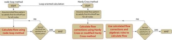
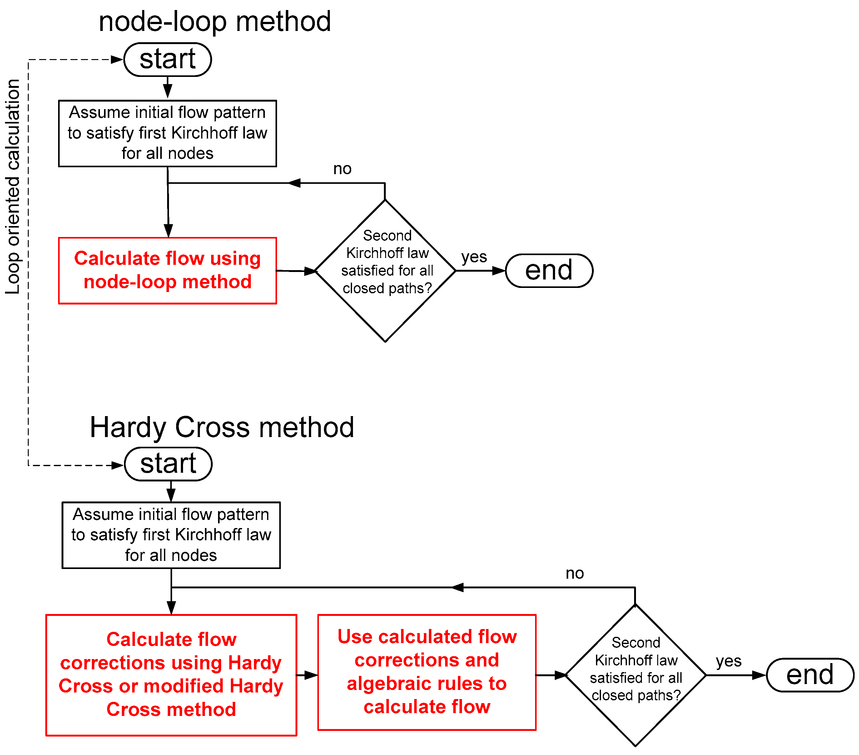
Since the development of the loop-oriented and node-oriented methods, and the introduction of matrix calculus, all the necessary tools are available to form a new innovative method [22,23]. This transformation makes it possible to calculate final flow in each iteration directly, and not by a correction of flow as in the aforementioned methods (Figure 1). Unfortunately, as already explained, these corrections of flow calculated using previous methods should be added to or subtracted from flow (or pressure in the node method) calculated in previous iterations according to complicated algebraic rules [3].
So, the main strength of the node-loop method introduced in 1972 by Wood and Charles [22] for waterworks calculation is not reflected in a noticeably reduced number of iterations compared to the modified Hardy Cross method. The main advantage of this method is in the capability to compute directly the pipe flow rate rather than to estimate a flow correction. The method uses a linear head loss term which allows a network of n pipes to be described by a set of n linear equations, which can be solved simultaneously for the flow distribution. In 1981 Wood and Rayes introduced an improvement in the node-loop method [23]. Here, will be shown the improved version of this method rearranged for gas flow and for water flow in terms of pressure distribution rather than head distribution (of which the quantity is expressed in length; such as elevation of water).
3. A Literary Overview of Existing Methods for Calculation of Flow Distribution in A Looped Network of Pipes
This section includes a literary overview of pipeline network models for water, gas and natural ventilation flow problems.
The excellent example of calculation of a looped natural gas distribution network after the original Hardy Cross method can be found in the Gas Engineers Handbook from 1974 [4]. The aforementioned algebraic rules for the correction of flow calculated as an intermediate step in an iterative procedure can be found in the reference book [4]. These rules can be used for both versions of the Hardy Cross method, and also for a general node-oriented method in which the correction of pressure is calculated as an intermediate step rather than as a correction of flow. These algebraic rules were further developed in Brkić [3]. The same spatial gas network as shown in Brkić [3] will also be used here for calculations of the node-loop method. Moreover, in this paper, as a comparison for the results obtained for liquid flow, the same topology of the network with same diameter of pipelines will be used for calculation of water flow.
Another excellent book on this issue, but only for waterworks calculation given by Boulos et al. [24] can be recommended for further reading. In this book, unfortunately, an obsolete relation given by the Hazen–Williams equation is used to correlate only water flow, pressure drops in pipes and hydraulics frictions.
Further, for details on natural ventilation airflow networks one can consult the paper of Aynsley [6]. As there is no space to calculate separately an air ventilation network, readers interested in this matter can make this in a very effective way, according to natural gas and water flow calculation shown in this paper. Specific details on airflow resistances are also given in Aynsley [6].
Moreover, conservation of energy for each pipe of water networks is done by Todini and Pilati [25], while gas networks are analyzed by Hamam and Brameller [26]. As a result, besides flow correction in each pipe, the pressure drop can also be simultaneously calculated. This method is also known as a hybrid or gradient approach. Some comparisons of available methods for pipeline network calculations can be found in Mah [27], Mah and Shacham [28], Mah and Lin [29], etc. To compare calculation of water networks using the Hazen-Williams equation and approaches with pseudo-loops, consult the book of Boulous et al [24]. Lopes [30] also deals with the program for the Hardy Cross solution of piping networks. Such problems today can be solved very easily using MS Excel [31,32].
4. Hydraulics Resistance of a Single Pipe
A source-issue that causes a problem with the calculation of hydraulic networks is the non-constant value of hydraulic resistance when fluid is conveyed through the pipe. Conversely, the electrical resistance of a wire or a resistor has a constant value, which has a consequence; non-iterative calculation of electrical circuits. However, this assumption is valid only for simplified DC Electric Power System models, whereas for more detailed AC models, a non-iterative calculation is required. To establish a relation between the flow rate of natural gas through a single pipe and the related pressure drop, the Renouard equation for gas flow will be used (1) [29]. Using this approach, the resistance will not be calculated at all, since the Renouard’s equation relates pressure and flow rates using other properties, parameters and quantities. On the other hand, for the calculation of the hydraulic resistance in a single pipe, the well-known Colebrook equation will be used [30]. The Colebrook equation is also iterative and can cause numerical problems [35,36,37,38] The pressure drop is calculated using the Darcy–Weisbach equation. Finally, for calculation of air-flow through a ventilation system, one can consult Aynsley [6], as previously mentioned.
The Hazen–Williams equation, which is used in the herein recommended book of Boulos et al. [24], is useless for calculation of gas flow. Introduced in the early 1900s, the Hazen–Williams equation determines the pipe friction head loss for water, requiring a single roughness coefficient (roughness is also a very important parameter in the Darcy–Weisbach scheme for calculation [39]). Unfortunately, even for water, the Hazen–Williams equation may produce errors as high as ±40% when applied outside a limited and somewhat controversial range of the Reynolds numbers, pipe diameters, and coefficients. Not only inaccurate, the Hazen–Williams equation is conceptually incorrect [40].
5. Topology of Looped Pipe Systems
Firstly, the maximal consumption per node, including one or more inlet nodes, has to be determined (red in Figure 2). These parameters are looked up during the calculation. Further, an initial guess of flow per conduit must be assigned to satisfy Kirchhoff’s first laws, and so chosen values are used for the first iteration [3]. Final flows do not depend on the first assumed flows per pipe (the countless initial flow pattern can satisfy Kirchhoff’s first law, and all of them can equally be used with the same final results [3,41]). After the iteration procedure is completed, and if the value of gas or water flow velocity for all conduits is below standard values, calculated flows become flow distribution per pipe for maximal possible consumption per node. Further, pressure per all nodes (can be heads in the case of water) can be calculated. The whole network can be supplied by gas or water from one or more points (nodes). The distribution network must be designed for the largest consumption assigned to network nodes, in order to maximize gas or water consumption of households. In reality households are located near a pipeline and they are connected to it, while in the model, consumption of a group of the houses is assigned to a node. The main purpose of the method is to calculate the flow pattern per pipe and the pressure pattern per node for the maximal load of the network.
The problem can be treated as inverse, i.e., flow per pipe assigned in the first iteration is not only the initial pattern, see (17). This flow pattern is not variable in further calculations. Instead of flows per pipe, which are now constants, pipe diameters become variables, and according to this approach, optimized pipes’ diameters in the network are the final result of the calculation (see Section 8 of this paper).
The first assumed flow pattern has to be chosen to satisfy Kirchhoff’s first law (continuity of flow), which means that the algebraic sum of flows per each node must be exactly zero. On the other hand, Kirchhoff’s second law (continuity of potential), which means that the algebraic sum of pressure drops per each contour, must be approximately zero at the end of the iterative procedure. The procedure can be interrupted when the algebraic sum of all nodes becomes approximately zero, or when flows per pipes are not changed in calculation after two successive iterations.
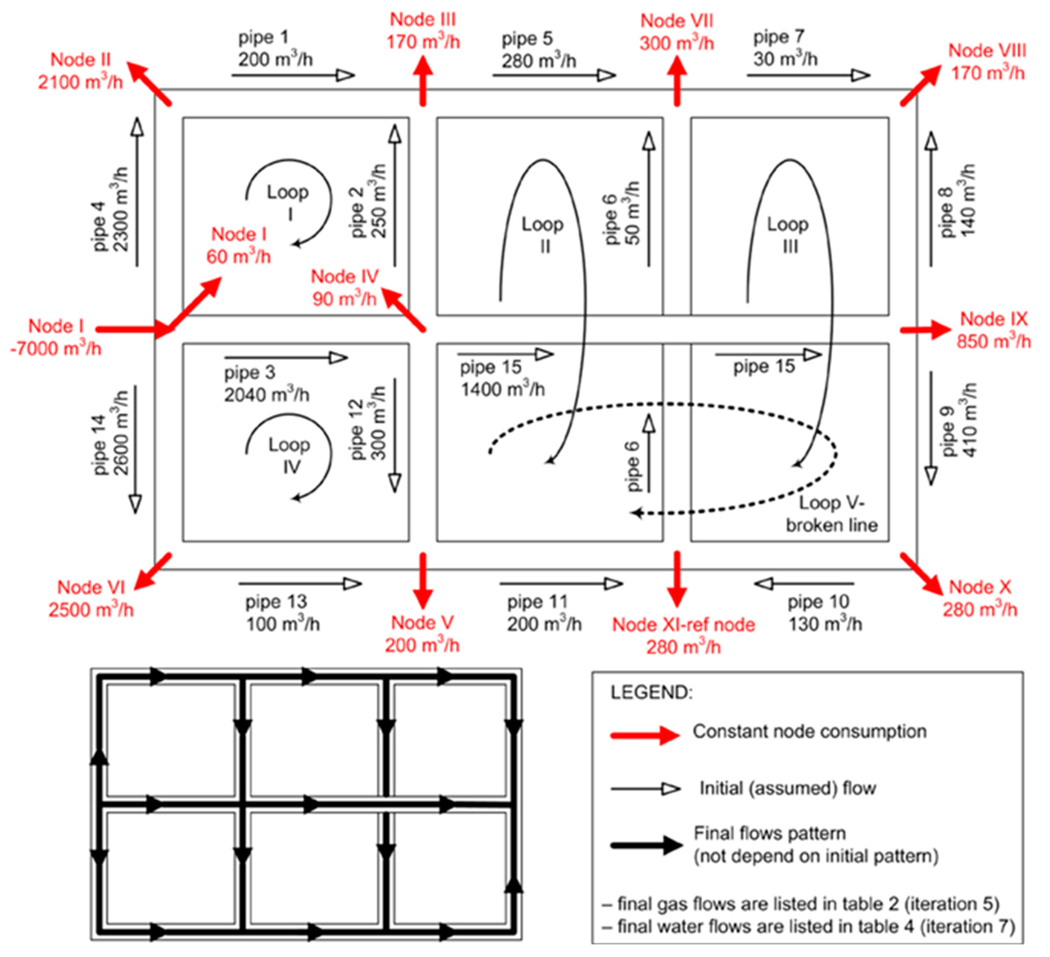
One spatial fluid distribution network of pipelines will be examined as an example (Figure 2). Polyvinyl chloride pipes (PVC) are used in the example shown in this paper.
The first step in solving a problem is to make a network map showing pipe sizes and lengths, connections between pipes (nodes), and sources of supply. For convenience in locating pipes, a code number is assigned to each loop and each pipe. Some of the pipes are mutual to one loop and some to two, or even three contours (i.e., pipe 12 belongs to the loops II, IV, and V). Special cases may occur, when two pipes cross each other but are not connected (like pipes 6 and 15), resulting in certain pipes being common to three or more loops. The distribution network then becomes three-dimensional (which is rare for gas with the exception of perhaps some chemical engineering facilities, water networks or district heating systems, and usually for airflow networks). For example, loop V consists of conduits 15, 9, 10, via 11, and 12. Gas/water flow into the network from a source on the left side is 7000 m3/h, and points of delivery are at junctions of pipes (nodes), with the red arrows pointing to volumes delivered (node consumption). Summation of these deliveries equals 7000 m3/h. Assumed gas flows and their directions are indicated by black arrows near the pipes (Figure 2).
6. Topology Equations for the Observed Looped Network of Pipes
When the network map with its pipe and loop numbers, and delivery and supply data is prepared, a mathematical description of the network can be made. To introduce the matrix form in calculations, it is necessary to represent the distribution network from Figure 2 as a graph according to Euler’s theorem from mineralogy (number of polyhedral angles and edges of minerals). The graph has X branches and Y nodes, where in Figure 2, X = 15 and Y = 11. The graph with n nodes (in our case 11) has Y-1 independent nodes (in our case 10) and X-Y+1 independent loops (in our case 5). The tree is a set of connected branches chosen to connect all nodes, but not to make any a closed path (not forming a loop). Branches which do not belong to a tree are links (number of links are X-Y+1). Loops in the network are formed using pipes from the tree and one more chosen from among the link pipes. The number of the loops is determined by the number of links. In the graph, one node is referent and all others are so called dependent nodes. In approaches with no referent node, one pseudo-loop must be introduced [44] which is very complicated and should be avoided. In Figure 2 the referent node is XI.
6.1. Loop Equations
The Renouard Equation (1) will be used for calculation of pressure drop in pipes in the case of natural gas distribution [46].
Regarding to the Renouard Formula (1) one has to be careful, since it does not relate pressure drop but actually difference of the quadratic pressure at the input and the output of the conduit. This means that is not actually a pressure drop despite using the same unit of measurement, i.e., the same unit is used as for pressure (Pa). Rather the parameter can be noted as pseudo-pressure drop. The fact that when this consecutive means that also is very useful for calculation of a gas pipeline with loops. So, the notation for pseudo-pressure drop is ambiguous [3] (only or with an appropriate index should be used instead of ).
The first derivative of the previous relation, where flow is treated as a variable is (2):
The Colebrook–White Equation (3) will be used for calculation of the Darcy friction factor in the case of water distribution [47]. The Colebrook-White equation is implicit in the friction factor, and here it is solved using MS Excel.
The friction factor calculated after Colebrook’s relation will be incorporated into the Darcy–Weisbach relation to calculate pressure drop in a water network (4).
Similarly, to the gas pipe-lines, the first derivate of the previous relation where the flow is treated as a variable is (5):
Then, according to the previous, for the gas network from Figure 2, a set of loop equations can be written as (6):
Previous relations can be noted in a matrix form as (7):
Or for waterworks or district heating systems from Figure 2 can be noted as (8):
i.e., in the matrix form for water distribution (9).
In the left matrix of the relations (7) and (9), rows represent loops and columns represent pipes. These relations are matrix reformulation of Kirchhoff’s second law. The sign for the term relates if the assumed flow is clockwise (1) or counterclockwise (−1) relative to the loop.
6.2. Node Equations
For all nodes in the network from Figure 2, relations after Kirchhoff’s first law can be noted as (10):
Or in a matrix form as (11) where the first matrix rows represents nodes excluding the referent node (For a formulation where node 1 is the referent node see Brkić [3]). The node matrix with all nodes included is not linearly independent. To obtain linear independence, any row of the node matrix can be omitted. Consequently, no information on the topology will be lost [26].
The first row corresponds to the first node, etc. The last row is for node 10 from Figure 2, as node 11 is chosen to be the referent one, and therefore must be omitted from the matrix. For example, node 1 has a connection with other nodes via pipes 3, 4 and 14, and for the first assumed flow pattern, all flows are from node 1 via connected pipes to other nodes. Therefore, terms 3, 4, and 14 in the first row are −1. Other pipes are not connected with node 1, and therefore all other terms in the first row of the node matrix are 0.
Note that there is no difference in cases of water apropos gas calculation when the node equations are observed.
7. Network Calculation According to The Node-Loop Method
The nodes and the loops equations previously shown will be here united in one coherent system by coupling these two sets of equations. This method will be examined in detail for the network shown in Figure 2. This network will be treated as a natural gas network in Section 7.1 and as a water network in Section 7.2, respectively. This approach also gives a good insight into the differences, which can occur in the cases of distribution of liquids apropos gaseous fluids.
7.1. The Node-Loop Calculation of Gas Networks
The first iteration for the gas calculation for the network from Figure 2 is shown in Table 1. If the sign of calculated flow is negative, this means that the flow direction from the previous iteration must be changed, otherwise, the sign must remain unchanged. In Table 1, loop and pipe numbers are listed in the first and the second column, respectively. The pipe length expressed in meters is listed in the third column, and assumed gas flow in each pipe expressed in m3/s is listed in the fourth column. The 1 or −1 in the fifth column indicates preceding flow in the fourth column. The plus or minus preceding the flow, Q, indicates the direction of the pipe flow for the particular loop. A plus sign denotes clockwise flow in the pipe within the loop, whereas a minus sign denotes anticlockwise flow in the pipe within the loop. All these assumptions will also be used in the case of waterworks and district heating system calculations.
To introduce the matrix calculations, the node-loop matrix [NL], the matrix of calculated flow in the observed iteration [Q], and [V] matrix in the right side of (12) will be defined.
The first ten rows in the NL (13) matrix are taken from the node matrix (11), whereas the next five rows are taken from the loop matrix (7 and 9). These five rows from the loop matrix are multiplied by the first derivate of the pressure drop function (2) from Table 1 for gas (column F’) (For water (5) and Table 2). Calculation from Table 1 is given in MS Excel Table S1: Gas, and from Table 2 in Table S2: Water, both given in Appendix A.
The first ten rows in the matrix [V] are node consumption (The right side of (11), node consumptions with a positive and input for node 1 with a negative sign from Figure 2 are expressed in m3/s) values, and the rest five terms are from Table 1; (14).
Solution of matrix [Q] is now (15):
The negative sign in front of some terms means that the sign preceding this term from the previous iteration must be changed.
Five iterations are enough for the calculation of the gas network from Figure 2. Calculated flows for these first five iterations will be listed in Table 3.
The flow direction is changed in pipes 2, 6, 8, 9 and 10 (opposite to the first assumed flows). Note that velocities in the last column of Table 3 are listed. Gas pressure in the network is circa 4 × 10⁵ Pa abs. Flow velocity per pipe is not balanced. Somewhere flow velocity is too small (Pipe 6: 0.05 m/s) whereas somewhere is too high (Pipe 4: 3.17 m/s). The whole task can be treated now as an inverse problem by fixing the flows per pipes and by optimizing pipe diameters as noted in Section 8. This can be done using the here presented node-loop method, Hardy Cross, or similar available methods (note that different pressure values in the gas network apropos the water network cause different values of gas speed compared to values of water speed; last column in Table 2 and Table 4, respectively).
7.2. The Node-Loop Calculation of Waterworks or District Heating Systems
8. A Note on The Optimization Problem
The Renouard Formula (1) for conditions in gas distribution networks assumes a constant density of a fluid within the conduits. This assumption only applies to incompressible flow, i.e., for liquid flows such as in water distribution systems for municipalities (or any other liquid, like crude oil, etc.). For the small pressure drops in typical gas distribution networks, the gas density can be treated as constant, which means that the gas can be treated as an incompressible fluid. The assumption of the incompressibility of the gas means that the gas is already compressed and forced to convey through conduits, but inside the pipeline system a pressure drop of the already compressed gas is minor and hence further changes of the gas density can be neglected. The fact is that the gas is actually compressed. Consequently, the volume of gas is decreased and then such compressed volume of gas is conveying with a constant density through the gas distribution pipeline. So, the mass of the gas is constant, but the volume is decreased while the gas density is, according to this, increased. The operational pressure for a typical distribution gas network is 4 × 10⁵ Pa abs i.e., 3 × 10⁵ Pa gauge and accordingly the volume of the gas is decreased four times compared to the volume of the gas in normal (standard) conditions. But the operational pressure for the gas distribution network can be lower (this case is valid for the network in the paper of Brkić [3]). This is not typical for natural gas distributive networks. This was a common practice in obsolete systems for distribution of city gas derived from coal [34]. So, flow in the Renourad Formula (1) adjusted for natural gas is usually expressed in normal (standard) conditions. Consequently, if flows in the previous paper of Brkić [3] are expressed in their real (compressed) values, and if these real values are numerically equalized with values expressed for normal (standard) conditions, this means that the operational pressure in the gas network is normal (standard). Otherwise, velocities in the previous paper of Brkić [3] have to be corrected. Velocities in the previous paper of Brkić [3] are calculated to be comparable with the procedure shown in Manojlović et al. [43], where calculations of the gas distribution network in the Serbian town Kragujevac is discussed. In Manojlović et al. [43], flows are expressed in their real values and not for normal or standard conditions of pressure as the common practice is. This network can be calculated to work with lower pressures, which is typical for gasses derived from coal. The second assumption can be rejected as less possible because in the part of Serbia south of the rivers Sava and the Danube where Kragujevac is situated, such gas was never used and especially not in the 1990s. Some comments about that issue were also made in Brkić [5]. So, to avoid any further ambiguity, the conclusion is that all flows in the previous paper of Brkić [3] are expressed in their real (compressed) values while operational pressure at the inputs of shown networks is normal (standard).
If these values of flows are noted for normal (standard) conditions of pressure as the common practice is (Table 3), while operational pressure is 4 × 10⁵ Pa abs i.e., 3 × 10⁵ Pa gauge, velocities of gas are different than those in the previous paper of Brkić [3], while flows remain unchanged.
Velocities in Table 3 are calculated using (16):
Now, for such values of flow, diameters of conduits are too large, and in such cases the Hardy Cross method [1] as well as the improved Hardy Cross method [2,3] can be used for optimization of diameters of conduits as shown in Figure 2. In a problem of optimization of pipe diameters, in the Renouard Formula (1), flow is no longer treated as a variable (17), while correction Δ is now the correction of diameters.
Ambiguity related to pressure conditions in a gas distributive network can cause very different and large consequences for the interpretation of calculated results.
A similar analogy regarding water networks is clear (18):
Diameters of conduits in the presented gas pipeline should be optimized, while diameters in the water network are within an accepted tolerance.
9. Main Advantages of The Node-Loop Method
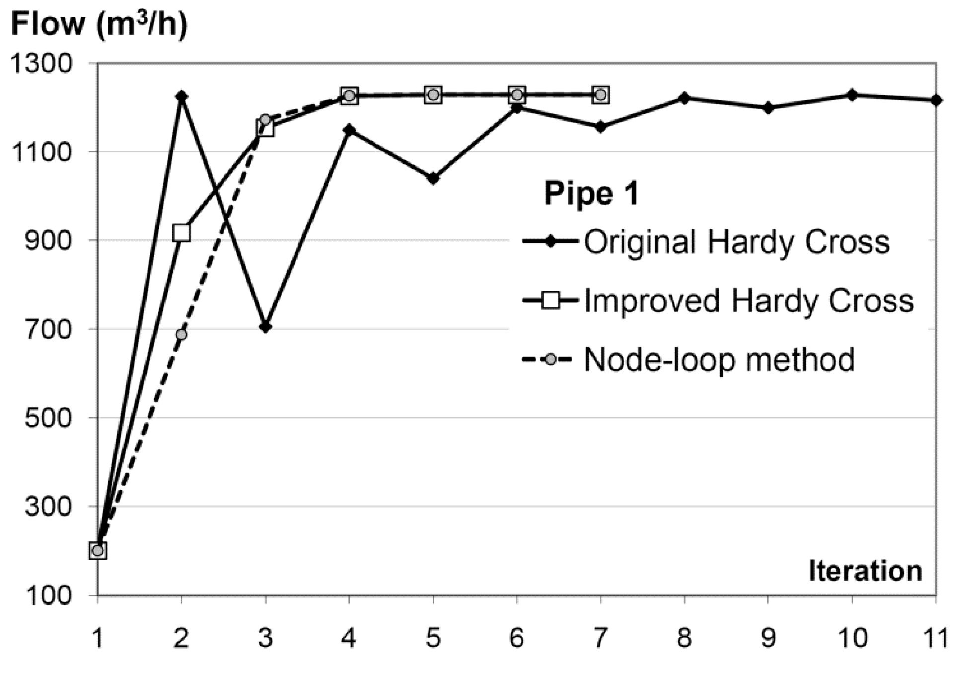
Figure 3 includes a validation of results. Two Hardy Cross methods are compared with the here described Node-loop method. We can also observe that the new Node-loop method and the modified Hardy Cross method [3] obtain an accurate solution after fourth iteration. Having increased the number of iterations, the solution of the new Node-loop method remains unchanged. In contrary, the original Hardy Cross method requires at least 10 iterations. Similar numbers of iterations are necessary to achieve the demanded accuracy in calculation as in the modified Hardy Cross method (Results for the Hardy Cross calculations are from the paper of Brkić [3]) (Figure 3). However, the novel Node-loop method does not need a complex algebraic scheme for the sign of flow corrections. This fact is the main advantage of the new Node-loop method.
The hydraulic computations involved in the design of water or gas distribution systems can only be approximated, as it is impossible to consider all factors affecting loss of head in a complicated network of pipes [48,49,50,51,52]. The here presented methods can easily be readapted for the detection of a position of leakage in a pipe network [51,52,53,54,55].
10. Conclusions
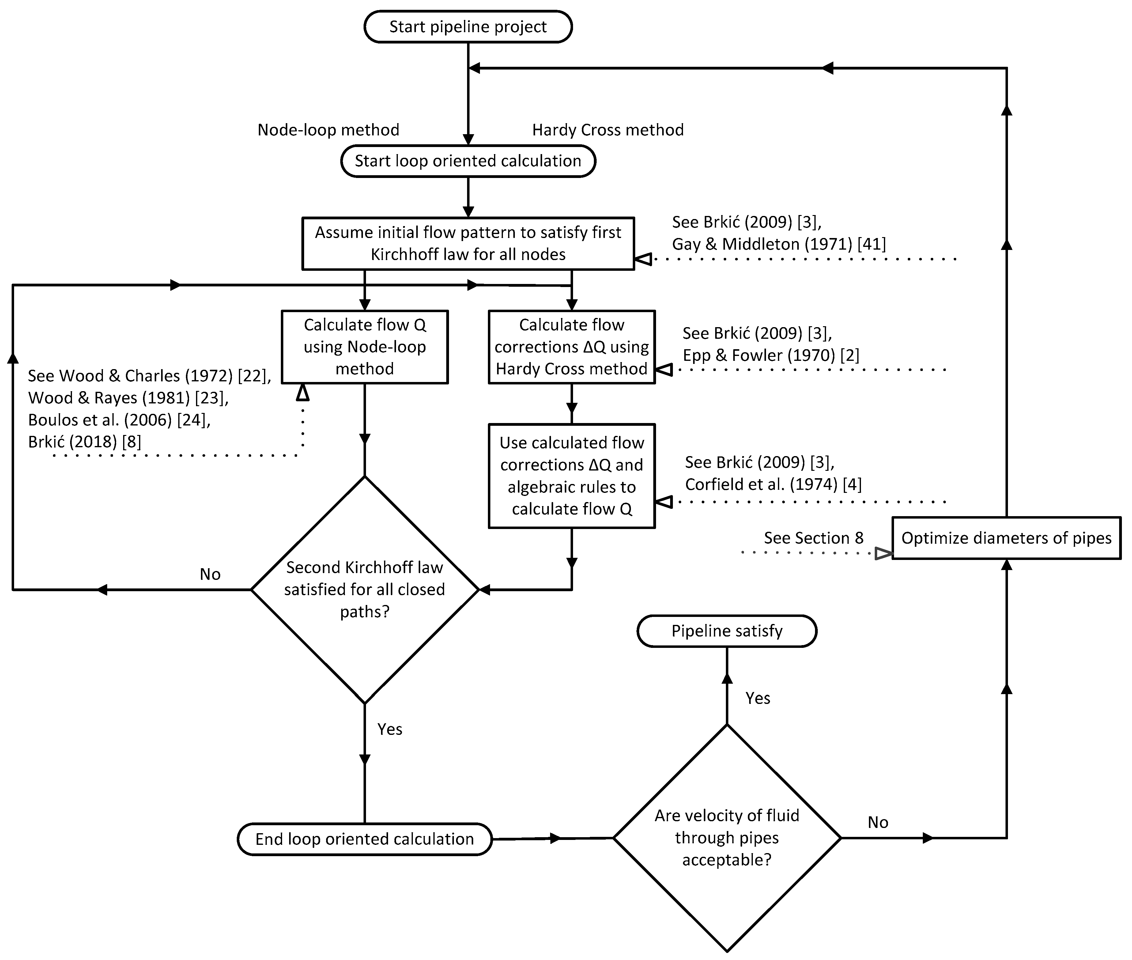
The here presented node-loop method is a powerful numerical procedure for calculation of flows or diameters as inverse problems in looped fluid distribution networks. The main advantage of the novel node-loop method is that flow in each pipe can be calculated directly, which is not possible for the original Hardy Cross nor the improved Hardy Cross methods (Figure 4).
Supplementary Materials
The following are available online at https://0-www-mdpi-com.brum.beds.ac.uk/2311-5521/4/2/73/s1, Table S1: Gas, Table S2: Water.
Author Contributions
The paper is a product of the joint efforts of the authors who worked together on models of natural gas distribution networks. P.P. has scientific background in applied mathematics and programming while D.B.’s background is in control and applied computing in mechanical and petroleum engineering. D.B. performed calculations with advice from P.P. who has extensive experience with implementation of probabilistic gas network modelling tools.
Funding
This work was partially supported by the Ministry of Education, Science and Technological Development of the Republic of Serbia through the project iii44006 and by the Ministry of Education, Youth and Sports of the Czech Republic through the National Programme of Sustainability (NPS II) project “IT4Innovations excellence in science-LQ1602”.
Acknowledgments
We thank John Cawley from IT4Innovations National Supercomputing Center, who as a native speaker kindly checked the correctness of English expressions throughout the paper.
Conflicts of Interest
The authors declare no conflict of interest. Neither the Alfatec, VŠB—Technical University of Ostrava nor any person acting on behalf of them is responsible for the use which might be made of this publication.
Nomenclature
| p | pressure (Pa) |
| ρr | relative gas density (-) |
| L | pipe length (m) |
| Q | fluid flow rate (m3/s) |
| pipe diameter (m) | |
| Re | Reynolds number (-) |
| ε | absolute roughness of inner pipe surface (m) |
| ρ | water density (kg/m3) |
| υ | velocity (m/s) |
| λ | Darcy (i.e., Moody or Darcy-Weisbach) friction factor (-) |
| F | pressure function (Pa for water, and Pa2 for natural gas) |
| pseudo-pressure drop (Pa) | |
| Subscripts: | |
| n | normal |
| w | water |
| g | gas |
| a | absolute |
| Constants: | |
| π ≈ 3.1415 | |
Appendix A
The whole calculation of water (‘water DB’) and gas (‘gas DB’) network from Figure 2 is available in two Excel files attached as Supplementary material.
To allow the necessary implicit calculations necessary for the Colebrook-White equation in Excel, press the ‘Office button’ at the upper-left corner of the Excel screen, and in the ‘Excel options’ choose ‘Formulas’ and finally tick the box ‘Enable iterative calculation’. This allows the implementation of so-called ‘Circular references’ into the calculations. The implicit Colebrook-White equation in the here presented example is used for water calculations, and hence this setup should only be used in the file ‘water DB’. To enter the input matrix expressed by the array formula in Excel, the range of the matrix must be selected starting with the cell in which the formula is typed. Then the function button F2 on the keyboard has to be pressed, and then press simultaneously CTRL+SHIFT+ENTER. If the formula is not entered as an array formula, the single result will appear (the first row and the first column of the matrix). This procedure is explained in Brkić [56,57]. Matrix calculations are used in both files; ‘water DB’ and gas ‘gas DB’. All previous details have been explained for MS Excel ver. 2007 (Enterprise edition).
References
- Cross, H. Analysis of Flow in Networks of Conduits or Conductors; University of Illinois at Urbana Champaign, College of Engineering Engineering Experiment Station: College Station, TX, USA, 1936; Available online: http://hdl.handle.net/2142/4433 (accessed on 1 March 2019).
- Epp, R.; Fowler, A.G. Efficient code for steady-state flows in networks. J. Hydraul. Div. Am. Soc. Civ. Eng. 1970, 96, 43–56. [Google Scholar]
- Brkić, D. An Improvement of Hardy Cross method applied on looped spatial natural gas distribution networks. Appl. Energy 2009, 86, 1290–1300. [Google Scholar] [CrossRef]
- Corfield, G.; Hunt, B.E.; Ott, R.J.; Binder, G.P.; Vandaveer, F.E. Distribution design for increased demand. In Gas Engineers Handbook; Segeler, C.G., Ed.; Chapter 9; Industrial Press: New York, NY, USA, 1974; pp. 63–83. [Google Scholar]
- Brkić, D. A Gas Distribution network hydraulic problem from practice. Petr. Sci. Technol. 2011, 29, 366–377. [Google Scholar] [CrossRef]
- Aynsley, R.M. A Resistance approach to analysis of natural ventilation airflow networks. J. Wind Eng. Ind. Aerodyn. 1997, 67–68, 711–719. [Google Scholar] [CrossRef]
- Kassai, M.; Poleczky, L.; Al-Hyari, L.; Kajtar, L.; Nyers, J. Investigation of the energy recovery potentials in ventilation systems in different climates. Facta Univ. Ser. Mech. Eng. 2018, 16, 203–217. [Google Scholar] [CrossRef]
- Brkić, D. Discussion of “Economics and statistical evaluations of using Microsoft Excel Solver in pipe network analysis” by I. A. Oke, A. Ismail, S. Lukman, S.O. Ojo, O.O. Adeosun, and M. O. Nwude. J. Pipeline Syst. Eng. Pract. 2018, 9, 7018002. [Google Scholar] [CrossRef]
- Del Hoyo Arce, I.; Herrero López, S.; López Perez, S.; Rämä, M.; Klobut, K.; Febres, J.A. Models for Fast Modelling of District Heating and Cooling Networks. Renew. Sustain. Energy Rev. 2018, 82, 1863–1873. [Google Scholar] [CrossRef]
- Elaoud, S.; Hafsi, Z.; Hadj-Taieb, L. Numerical modelling of hydrogen-natural gas mixtures flows in looped networks. J. Petr. Sci. Eng. 2017, 159, 532–541. [Google Scholar] [CrossRef]
- Nikolić, B.; Jovanović, M.; Milošević, M.; Milanović, S. Function k-as a link between fuel flow velocity and fuel pressure, depending on the type of fuel. Facta Univ. Ser. Mech. Eng. 2017, 15, 119–132. [Google Scholar] [CrossRef]
- Shamir, U.; Howard, C.D.D. Water distribution systems analysis. J. Hydraul. Div. Am. Soc. Civ. Eng. 1968, 94, 219–234. [Google Scholar]
- Brkić, D. Iterative methods for looped network pipeline calculation. Water Resour. Manag. 2011, 25, 2951–2987. [Google Scholar] [CrossRef]
- Niazkar, M.; Afzali, S.H. Analysis of water distribution networks using MATLAB and Excel spreadsheet: Q-based methods. Comput. Appl. Eng. Educ. 2017, 25, 277–289. [Google Scholar] [CrossRef]
- Niazkar, M.; Afzali, S.H. Analysis of water distribution networks using MATLAB and Excel spreadsheet: H-based methods. Comput. Appl. Eng. Educ. 2017, 25, 129–141. [Google Scholar] [CrossRef]
- Spiliotis, M.; Tsakiris, G. Water distribution system analysis: Newton-Raphson method revisited. J. Hydraul. Eng. 2011, 137, 852–855. [Google Scholar] [CrossRef]
- Brkić, D. Discussion of “Water distribution system analysis: Newton-Raphson method revisited” by M. Spiliotis and G. Tsakiris. J. Hydraul. Eng. 2012, 138, 822–824. [Google Scholar] [CrossRef]
- Spiliotis, M.; Tsakiris, G. Closure to “Water distribution system analysis: Newton-Raphson method revisited” by M. Spiliotis and G. Tsakiris. J. Hydraul. Eng. 2012, 138, 824–826. [Google Scholar] [CrossRef]
- Simpson, A.; Elhay, S. Jacobian matrix for solving water distribution system equations with the Darcy-Weisbach head-loss model. J. Hydraul. Eng. 2011, 137, 696–700. [Google Scholar] [CrossRef]
- Brkić, D. Discussion of “Jacobian matrix for solving water distribution system equations with the Darcy-Weisbach head-loss model” by Angus Simpson and Sylvan Elhay. J. Hydraul. Eng. 2012, 138, 1000–1001. [Google Scholar] [CrossRef]
- Simpson, A.R.; Elhay, S. Closure to “Jacobian matrix for solving water distribution system equations with the Darcy-Weisbach head-loss model” by Angus Simpson and Sylvan Elhay. J. Hydraul. Eng. 2012, 138, 1001–1002. [Google Scholar] [CrossRef]
- Wood, D.J.; Charles, C.O.A. Hydraulic network analysis using linear theory. J. Hydraul. Div. Am. Soc. Civ. Eng. 1972, 98, 1157–1170. [Google Scholar]
- Wood, D.J.; Rayes, A.G. Reliability of algorithms for pipe network analysis. J. Hydraul. Div. Am. Soc. Civ. Eng. 1981, 107, 1145–1161. [Google Scholar]
- Boulos, P.F.; Lansey, K.E.; Karney, B.W. Comprehensive Water Distribution Systems Analysis Handbook for Engineers and Planners, 2nd ed.; MWH: Broomfield, CO, USA, 2006. [Google Scholar]
- Todini, E.; Pilati, S. A gradient method for the analysis of pipe networks. In Computer Applications in Water Supply; Coulbeck, B., Orr, C.H., Eds.; John Wiley & Sons Research Studies Press: London, UK, 1988; pp. 1–20. [Google Scholar]
- Hamam, Y.M.; Brameller, A. Hybrid method for the solution of piping networks. Proc. Inst. Electr. Eng. 1971, 118, 1607–1612. [Google Scholar] [CrossRef]
- Mah, R.S.H. Pipeline network calculations using sparse computation techniques. Chem. Eng. Sci. 1974, 29, 1629–1638. [Google Scholar] [CrossRef]
- Mah, R.S.H.; Shacham, M. Pipeline network design and synthesis. Adv. Chem. Eng. 1978, 10, 125–209. [Google Scholar] [CrossRef]
- Mah, R.S.H.; Lin, T.D. Comparison of Modified Newton’s methods. Comput. Chem. Eng. 1980, 4, 75–78. [Google Scholar] [CrossRef]
- Lopes, A.M.G. Implementation of the Hardy-Cross method for the solution of piping networks. Comput. Appl. Eng. Educ. 2004, 12, 117–125. [Google Scholar] [CrossRef]
- Huddleston, D.H.; Alarcon, V.J.; Chen, W. Water Distribution network analysis using Excel. J. Hydraul. Eng. 2004, 130, 1033–1035. [Google Scholar] [CrossRef]
- Brkić, D. Spreadsheet-Based Pipe Networks Analysis for Teaching and Learning Purpose. Spreadsheets Educ. 2016, 9, 4. Available online: https://sie.scholasticahq.com/article/4646-spreadsheet-based-pipe-networks-analysis-for-teaching-and-learning-purpose (accessed on 12 April 2019).
- Anonymous. Pipeline-network analyzer. J. Frankl. Inst. 1952, 254, 195. [Google Scholar] [CrossRef]
- Anonymous. Substitution of manufactured gas for natural gas. J. Frankl. Inst. 1930, 209, 121–125. [Google Scholar] [CrossRef]
- Brkić, D. Review of explicit approximations to the Colebrook relation for flow friction. J. Petr. Sci. Eng. 2011, 77, 34–48. [Google Scholar] [CrossRef]
- Brkić, D.; Ćojbašić, Ž. Evolutionary optimization of Colebrook’s turbulent flow friction approximations. Fluids 2017, 2, 15. [Google Scholar] [CrossRef]
- Praks, P.; Brkić, D. Choosing the optimal multi-point iterative method for the Colebrook flow friction equation. Processes 2018, 6, 130. [Google Scholar] [CrossRef]
- Brkić, D.; Praks, P. Accurate and Efficient Explicit Approximations of the Colebrook Flow Friction Equation Based on the Wright ω-Function. Mathematics 2019, 7, 34. [Google Scholar] [CrossRef]
- Brkić, D. Can Pipes be actually really that smooth? Int. J. Refrig. 2012, 35, 209–215. [Google Scholar] [CrossRef]
- Liou, C.P. Limitations and proper use of the Hazen-Williams equation. J. Hydraul. Eng. 1998, 124, 951–954. [Google Scholar] [CrossRef]
- Gay, B.; Middleton, P. The solution of pipe network problems. Chem. Eng. Sci. 1971, 26, 109–123. [Google Scholar] [CrossRef]
- Mathews, E.H.; Köhler, P.A.J. A Numerical optimization procedure for complex pipe and duct network design. Int. J. Numer. Methods Heat Fluid Flow 1995, 5, 445–457. [Google Scholar] [CrossRef]
- Manojlović, V.; Arsenović, M.; Pajović, V. Optimized design of a gas-distribution pipeline network. Appl. Energy 1994, 48, 217–224. [Google Scholar] [CrossRef]
- Chansler, J.M.; Rowe, D.R. Microcomputer analysis of pipe networks. Water Eng. Manag. 1990, 137, 36–39. [Google Scholar]
- Marušić-Paloka, E.; Pažanin, I. On the Viscous Flow through a long pipe with non-constant pressure boundary condition. Zeitschrift für Naturforschung A 2018, 73, 639–644. [Google Scholar] [CrossRef]
- Coelho, P.M.; Pinho, C. Considerations about equations for steady state flow in natural gas pipelines. J. Braz. Soc. Mech. Sci. Eng. 2007, 29, 262–273. [Google Scholar] [CrossRef]
- Colebrook, C.F. Turbulent flow in pipes, with particular reference to the transition region between the smooth and rough pipe laws. J. Inst. Civ. Eng. 1939, 11, 133–156. [Google Scholar] [CrossRef]
- Raoni, R.; Secchi, A.R.; Biscaia, E.C., Jr. Novel method for looped pipeline network resolution. Comput. Chem. Eng. 2017, 96, 169–182. [Google Scholar] [CrossRef]
- Oliva, G.; Rikos, A.I.; Hadjicostis, C.N.; Gasparri, A. Distributed Flow Network Balancing with Minimal Effort. IEEE Trans. Autom. Control 2019, in press. [Google Scholar] [CrossRef]
- Pambour, K.; Cakir Erdener, B.; Bolado-Lavin, R.; Dijkema, G. Development of a simulation framework for analyzing security of supply in integrated gas and electric power systems. Appl. Sci. 2017, 7, 47. [Google Scholar] [CrossRef]
- Praks, P.; Kopustinskas, V.; Masera, M. Probabilistic modelling of security of supply in gas networks and evaluation of new infrastructure. Reliab. Eng. Syst. Saf. 2015, 144, 254–264. [Google Scholar] [CrossRef]
- Pietrucha-Urbanik, K.; Tchorzewska-Cieslak, B. Water Supply System operation regarding consumer safety using Kohonen neural network. Safety, Reliability and Risk Analysis: Beyond the Horizon, 2014, 1115–1120. In Proceedings of the Advances in Safety, Reliability and Risk Management: ESREL, Amsterdam, The Netherlands, 29 September–2 October 2013. [Google Scholar] [CrossRef]
- Bermúdez, J.-R.; López-Estrada, F.-R.; Besançon, G.; Valencia-Palomo, G.; Torres, L.; Hernández, H.-R. Modeling and simulation of a hydraulic network for leak diagnosis. Math. Comput. Appl. 2018, 23, 70. [Google Scholar] [CrossRef]
- Adedeji, K.; Hamam, Y.; Abe, B.; Abu-Mahfouz, A. Leakage detection and estimation algorithm for loss reduction in water piping networks. Water 2017, 9, 773. [Google Scholar] [CrossRef]
- Pietrucha-Urbanik, K.; Żelazko, A. Approaches to assess water distribution failure. Period. Polytech. Civ. Eng. 2017, 61, 632–639. [Google Scholar] [CrossRef]
- Brkić, D. Determining friction factors in turbulent pipe flow. Chem. Eng. (N. Y.) 2012, 119, 34–39. [Google Scholar]
- Brkić, D. Solution of the implicit Colebrook Equation for Fflow friction Using Excel. Spreadsheets Educ. 2017, 10, 2. Available online: https://sie.scholasticahq.com/article/4663-solution-of-the-implicit-colebrook-equation-for-flow-friction-using-excel (accessed on 12 April 2019).
Figure 1.
The main strength of the node-loop method compared with the Hardy Cross method is in direct flow calculation.
Figure 1.
The main strength of the node-loop method compared with the Hardy Cross method is in direct flow calculation.

Figure 2.
An example of a spatial gas/water distribution network with loops.

Figure 3.
A comparison of the convergence properties for the Hardy Cross methods, the original and improved, and the new node-loop method.
Figure 3.
A comparison of the convergence properties for the Hardy Cross methods, the original and improved, and the new node-loop method.

Figure 4.
The main conceptual difference between the Hardy Cross method (the original and improved) and the node-loop method.
Figure 4.
The main conceptual difference between the Hardy Cross method (the original and improved) and the node-loop method.


Table 1.
Node-loop analysis for the gas network from Figure 1.
Table 1.
Node-loop analysis for the gas network from Figure 1.
| Loop | Pipe | (m) | L (m) | a Q (m3/s) | Sign (Q) | c F | d |F’| |
|---|---|---|---|---|---|---|---|
| I | 1 | 0.4064 | 100 | b A1 = 0.0556 | +1 | 114959 | |a1| = 3766062 |
| 2 | 0.3048 | 100 | A2 = −0.0694 | −1 | −690438 | |a2| = 18094990 | |
| 3 | 0.1524 | 100 | A3 = −0.5667 | −1 | −889949040 | |a3| = 2858306918 | |
| 4 | 0.3048 | 100 | A4 = 0.6389 | +1 | 39193885 | |a4| = 111651451 | |
| Σ | A = −851330634 | ||||||
| II | 5 | 0.1524 | 100 | B1 = 0.0778 | +1 | 23969880 | |b1| = 560895181 |
| 6 | 0.3048 | 200 | B2 = −0.0139 | −1 | −73795 | |b2| = 9670144 | |
| 11 | 0.1524 | 100 | B3 = −0.0556 | −1 | −12993101 | |b3| = 425654001 | |
| 12 | 0.1524 | 100 | B4 = −0.0833 | −1 | −27176838 | |b4| = 593542132 | |
| 2 | 0.3048 | 100 | B5 = 0.0694 | +1 | 690438 | |b5| = 18094990 | |
| Σ | B = −15583417 | ||||||
| III | 7 | 0.1524 | 100 | C1 = 0.0083 | +1 | 411338 | |c1| = 89836237 |
| 8 | 0.1524 | 100 | C2 = −0.0389 | −1 | −6788773 | |c2| = 317714556 | |
| 9 | 0.3048 | 100 | C3 = 0.1139 | +1 | 1698792 | |c3| = 27147529 | |
| 10 | 0.1524 | 100 | C4 = 0.0361 | +1 | 5932191 | |c4| = 298982433 | |
| 6 | 0.3048 | 200 | C5 = 0.0139 | +1 | 73795 | |c5| = 9670144 | |
| Σ | C = 1327344 | ||||||
| IV | 3 | 0.1524 | 100 | D1 = 0.5667 | +1 | 889949040 | |d1| = 2858306918 |
| 12 | 0.1524 | 100 | D2 = 0.0833 | +1 | 27176838 | |d2| = 593542132 | |
| 13 | 0.1524 | 100 | D3 = −0.0278 | −1 | −3679919 | |d3| = 241108279 | |
| 14 | 0.4064 | 100 | D4 = −0.7222 | −1 | −12243919 | |d4| = 30854675 | |
| Σ | D = 901202040 | ||||||
| V | 15 | 0.1524 | 200 | E1 = 0.3889 | +1 | 897059511 | |e1| = 4198238510 |
| 9 | 0.3048 | 100 | E2 = 0.1139 | +1 | 1698792 | |e2| = 27147529 | |
| 10 | 0.1524 | 100 | E3 = 0.0361 | +1 | 5932191 | |e3| = 298982433 | |
| 11 | 0.1524 | 100 | E4 = −0.0556 | −1 | −12993101 | |e4| = 425654001 | |
| 12 | 0.1524 | 100 | E5 = −0.0833 | −1 | −27176838 | |e5| = 593542132 | |
| Σ | E = 864520555 |
a from Figure 2 but expressed in m3/s. b letters used in (13) and (14). c see (1). d see (2).
Table 2.
Node-loop analysis for the water network from Figure 2.
Table 2.
Node-loop analysis for the water network from Figure 2.
| Loop | Pipe | (m) | L (m) | a Q(m3/s) | Sign (Q) | c Re | d ε/δ | e λ | f F | g |F’| |
|---|---|---|---|---|---|---|---|---|---|---|
| I | 1 | 0.4064 | 100 | b A1 = 0.0556 | +1 | 195566.25 | 4.92 × 10⁻⁵ | 0.01609 | 363.1919278 | |a1| = 13074.9094 |
| 2 | 0.3048 | 100 | A2 = −0.0694 | −1 | 325943.75 | 6.56 × 10⁻⁵ | 0.01492 | −2217.677686 | |a2| = 63869.11737 | |
| 3 | 0.1524 | 100 | A3 = −0.5667 | −1 | 5319401.99 | 1.31 × 10⁻⁴ | 0.01290 | −4084603.502 | |a3| = 14416247.66 | |
| 4 | 0.3048 | 100 | A4 = 0.6389 | +1 | 2998682.50 | 6.56 × 10⁻⁵ | 0.01184 | 148932.0282 | |a4| = 466222.0014 | |
| Σ | A = −3937526 | |||||||||
| II | 5 | 0.1524 | 100 | B1 = 0.0778 | +1 | 730114.00 | 1.31 × 10⁻⁴ | 0.01423 | 84860.18126 | |b1| = 2182118.947 |
| 6 | 0.3048 | 200 | B2 = −0.0139 | −1 | 65188.75 | 6.56 × 10⁻⁵ | 0.01998 | −237.4945042 | |b2| = 34199.2086 | |
| 11 | 0.1524 | 100 | B3 = −0.0556 | −1 | 521510.00 | 1.31 × 10⁻⁴ | 0.01470 | −44732.90001 | |b3| = 1610384.4 | |
| 12 | 0.1524 | 100 | B4 = −0.0833 | −1 | 782265.00 | 1.31 × 10⁻⁴ | 0.01414 | −96832.35986 | |b4| = 2323976.637 | |
| 2 | 0.3048 | 100 | B5 = 0.0694 | +1 | 325943.75 | 6.56 × 10⁻⁵ | 0.01492 | 2217.677686 | |b5| = 63869.11737 | |
| Σ | B = −54725 | |||||||||
| III | 7 | 0.1524 | 100 | C1 = 0.0083 | +1 | 78226.50 | 1.31 × 10⁻⁴ | 0.01954 | 1338.024663 | |c1| = 321125.9191 |
| 8 | 0.1524 | 100 | C2 = −0.0389 | −1 | 365057.00 | 1.31 × 10⁻⁴ | 0.01531 | −22830.90776 | |c2| = 1174160.971 | |
| 9 | 0.3048 | 100 | C3 = 0.1139 | +1 | 534547.75 | 6.56 × 10⁻⁵ | 0.01391 | 5557.748158 | |c3| = 97599.47985 | |
| 10 | 0.1524 | 100 | C4 = 0.0361 | +1 | 338981.50 | 1.31 × 10⁻⁴ | 0.01545 | 19868.97118 | |c4| = 1100435.327 | |
| 6 | 0.3048 | 200 | C5 = 0.0139 | +1 | 65188.75 | 6.56 × 10⁻⁵ | 0.01998 | 237.4945042 | |c5| = 34199.2086 | |
| Σ | C = 4171 | |||||||||
| IV | 3 | 0.1524 | 100 | D1 = 0.5667 | +1 | 5319401.99 | 1.31 × 10⁻⁴ | 0.01290 | 4084603.502 | |d1| = 14416247.66 |
| 12 | 0.1524 | 100 | D2 = 0.0833 | +1 | 782265.00 | 1.31 × 10⁻⁴ | 0.01414 | 96832.35986 | |d2| = 2323976.637 | |
| 13 | 0.1524 | 100 | D3 = −0.0278 | −1 | 260755.00 | 1.31 × 10⁻⁴ | 0.01600 | −12174.73104 | |d3| = 876580.635 | |
| 14 | 0.4064 | 100 | D4 = −0.7222 | −1 | 2542361.25 | 4.92 × 10⁻⁵ | 0.01157 | −44129.48853 | |d4| = 122204.7375 | |
| Σ | D = 4125132 | |||||||||
| V | 15 | 0.1524 | 200 | E1 = 0.3889 | +1 | 3650569.99 | 1.31 × 10⁻⁴ | 0.01302 | 3882751.322 | |e1| = 19968435.37 |
| 9 | 0.3048 | 100 | E2 = 0.1139 | +1 | 534547.75 | 6.56 × 10⁻⁵ | 0.01391 | 5557.748158 | |e2|= 97599.47985 | |
| 10 | 0.1524 | 100 | E3 = 0.0361 | +1 | 338981.50 | 1.31 × 10⁻⁴ | 0.01545 | 19868.97118 | |e3| = 1100435.327 | |
| 11 | 0.1524 | 100 | E4 = −0.0556 | −1 | 521510.00 | 1.31 × 10⁻⁴ | 0.01470 | −44732.90001 | |e4| = 1610384.4 | |
| 12 | 0.1524 | 100 | E5 = −0.0833 | −1 | 782265.00 | 1.31 × 10⁻⁴ | 0.01414 | −96832.35986 | |e5| = 2323976.637 | |
| Σ | E = 3766613 |
a From Figure 2 but expressed in m3/s. b Letters used in (13) and (14). c Reynolds number; dynamic water viscosity 0.00089 Pas. d Relative roughness; absolute roughness ε = 0.00002 m for Polyvinyl chloride (PVC) pipes. e Friction factor (3) calculated using MS Excel. f Pressure drop in pipe (4). g See (5).
Table 3.
The first five iterations for the gas network from Figure 1.
Table 3.
The first five iterations for the gas network from Figure 1.
| Flow in m3/h | c Gas Velocity | ||||||
|---|---|---|---|---|---|---|---|
| Iteration | a 0 | 1 | 2 | 3 | 4 | b 5 | m/s |
| Pipe 1 | 200 | 687.38 | 1172.23 | 1225.74 | 1228.19 | 1228.19 | 0.66 |
| Pipe 2 | 250 | 33.55 | −307.01 | 360.38 | 362.80 | 362.80 | 0.35 |
| Pipe 3 | 2040 | 988.81 | 618.87 | 550.48 | 547.68 | 547.68 | 2.08 |
| Pipe 4 | 2300 | 2787.38 | 3272.23 | 3325.74 | 3328.19 | 3328.19 | 3.17 |
| Pipe 5 | 280 | 550.93 | 695.22 | 695.36 | 695.39 | 695.39 | 2.65 |
| Pipe 6 | 50 | 78.54 | −60.99 | 50.63 | 50.73 | 50.73 | 0.05 |
| Pipe 7 | 30 | 329.48 | 334.23 | 344.74 | 344.66 | 344.66 | 1.31 |
| Pipe 8 | 140 | −159.48 | 164.23 | 174.74 | 174.66 | 174.66 | 0.66 |
| Pipe 9 | 410 | 20.26 | −121.61 | 115.19 | 115.28 | 115.28 | 0.11 |
| Pipe 10 | 130 | −259.74 | 401.61 | 395.19 | 395.28 | 395.28 | 1.50 |
| Pipe 11 | 200 | 618.28 | 620.62 | 624.57 | 624.55 | 624.55 | 2.38 |
| Pipe 12 | 300 | 154.48 | 271.72 | 260.79 | 260.43 | 260.43 | 0.99 |
| Pipe 13 | 100 | 663.80 | 548.90 | 563.78 | 564.13 | 564.13 | 2.15 |
| Pipe 14 | 2600 | 3163.80 | 3048.90 | 3063.78 | 3064.13 | 3064.13 | 1.64 |
| Pipe 15 | 1400 | 710.78 | 564.16 | 560.07 | 560.05 | 560.05 | 2.13 |
a First assumed flows per pipes chosen after Kirchhoff’s first law (black letters in Figure 2). b Values in iteration 5 are equal to iteration 4, fulfilling the stopping criterion. c Gas velocity (10–15 m/s recommended); υ = (4·p·Q)/(δ2·π); where p = pn/pa = 0.25 and pa is the absolute pressure of gas in the pipeline, here pa = 400,000 Pa, and pn = normal pressure ~100,000 Pa, p = 400,000 Pa/100,000 Pa = 1/4.
Table 4.
The first seven iterations for the water network from Figure 2.
Table 4.
The first seven iterations for the water network from Figure 2.
| Flow in m3/h | Water Velocity m/s | ||||||||
|---|---|---|---|---|---|---|---|---|---|
| Iteration | a 0 | 1 | 2 | 3 | 4 | 5 | 6 | b 7 | |
| Pipe 1 | 200 | 619.22 | 1117.82 | 1205.89 | 1214.92 | 1215.25 | 1215.26 | 1215.26 | 2.6 |
| Pipe 2 | 250 | 69.21 | −260.68 | 345.80 | 354.68 | 355.00 | 355.01 | 355.01 | 1.4 |
| Pipe 3 | 2040 | 1071.47 | 671.88 | 567.12 | 556.60 | 556.22 | 556.21 | 556.21 | 8.5 |
| Pipe 4 | 2300 | 2719.22 | 3217.82 | 3305.89 | 3314.92 | 3315.25 | 3315.26 | 3315.26 | 12.6 |
| Pipe 5 | 280 | 518.43 | 687.14 | 690.09 | 690.24 | 690.25 | 690.25 | 690.25 | 10.5 |
| Pipe 6 | 50 | 90.95 | −57.70 | 43.41 | 43.11 | 43.10 | 43.10 | 43.10 | 0.2 |
| Pipe 7 | 30 | 309.38 | 329.44 | 346.68 | 347.13 | 347.15 | 347.15 | 347.15 | 5.3 |
| Pipe 8 | 140 | −139.38 | 159.44 | 176.68 | 177.13 | 177.15 | 177.15 | 177.15 | 2.7 |
| Pipe 9 | 410 | 47.60 | −115.49 | 113.24 | 113.39 | 113.39 | 113.39 | 113.39 | 0.4 |
| Pipe 10 | 130 | −232.40 | 395.49 | 393.24 | 393.39 | 393.39 | 393.39 | 393.39 | 6.0 |
| Pipe 11 | 200 | 603.35 | 617.79 | 629.83 | 630.28 | 630.29 | 630.29 | 630.29 | 9.6 |
| Pipe 12 | 300 | 154.04 | 267.49 | 262.84 | 261.80 | 261.76 | 261.76 | 261.76 | 4.0 |
| Pipe 13 | 100 | 649.31 | 550.30 | 566.99 | 568.48 | 568.53 | 568.54 | 568.54 | 8.7 |
| Pipe 14 | 2600 | 3149.31 | 3050.30 | 3066.99 | 3068.48 | 3068.53 | 3068.54 | 3068.54 | 6.6 |
| Pipe 15 | 1400 | 758.22 | 575.07 | 560.08 | 559.48 | 559.46 | 559.46 | 559.46 | 8.5 |
a First assumed flows per pipes chosen after Kirchhoff’s first law (black letters in Figure 2). b Values in iterations 7 are equal as in iteration 6, stopping criterion is fulfilled.
© 2019 by the authors. Licensee MDPI, Basel, Switzerland. This article is an open access article distributed under the terms and conditions of the Creative Commons Attribution (CC BY) license (http://creativecommons.org/licenses/by/4.0/).
Share and Cite
MDPI and ACS Style
Brkić, D.; Praks, P. An Efficient Iterative Method for Looped Pipe Network Hydraulics Free of Flow-Corrections. Fluids 2019, 4, 73. https://0-doi-org.brum.beds.ac.uk/10.3390/fluids4020073
AMA Style
Brkić D, Praks P. An Efficient Iterative Method for Looped Pipe Network Hydraulics Free of Flow-Corrections. Fluids. 2019; 4(2):73. https://0-doi-org.brum.beds.ac.uk/10.3390/fluids4020073
Chicago/Turabian StyleBrkić, Dejan, and Pavel Praks. 2019. "An Efficient Iterative Method for Looped Pipe Network Hydraulics Free of Flow-Corrections" Fluids 4, no. 2: 73. https://0-doi-org.brum.beds.ac.uk/10.3390/fluids4020073