Staggered Conservative Scheme for 2-Dimensional Shallow Water Flows


1
Industrial and Financial Mathematics Research Group, Faculty of Mathematics and Natural Sciences, Institut Teknologi Bandung, Jalan Ganesha 10, Bandung 40132, Indonesia
2
School of Computing, Telkom University, Jl. Telekomunikasi No. 01 Terusan Buah Batu, Bandung 40257, Indonesia
*
Author to whom correspondence should be addressed.
†
These authors contributed equally to this work.
Fluids 2020, 5(3), 149; https://0-doi-org.brum.beds.ac.uk/10.3390/fluids5030149
Submission received: 11 August 2020
/
Revised: 26 August 2020
/
Accepted: 27 August 2020
/
Published: 31 August 2020
(This article belongs to the Special Issue Mathematical and Numerical Modeling of Water Waves)
Abstract
:Simulating discontinuous phenomena such as shock waves and wave breaking during wave propagation and run-up has been a challenging task for wave modeller. This requires a robust, accurate, and efficient numerical implementation. In this paper, we propose a two-dimensional numerical model for simulating wave propagation and run-up in shallow areas. We implemented numerically the 2-dimensional Shallow Water Equations (SWE) on a staggered grid by applying the momentum conserving approximation in the advection terms. The numerical model is named MCS-2d. For simulations of wet–dry phenomena and wave run-up, a method called thin layer is used, which is essentially a calculation of the momentum deactivated in dry areas, i.e., locations where the water thickness is less than the specified threshold value. Efficiency and robustness of the scheme are demonstrated by simulations of various benchmark shallow flow tests, including those with complex bathymetry and wave run-up. The accuracy of the scheme in the calculation of the moving shoreline was validated using the analytical solutions of Thacker 1981, N-wave by Carrier et al., 2003, and solitary wave in a sloping bay by Zelt 1986. Laboratory benchmarking was performed by simulation of a solitary wave run-up on a conical island, as well as a simulation of the Monai Valley case. Here, the embedded-influxing method is used to generate an appropriate wave influx for these simulations. Simulation results were compared favorably to the analytical and experimental data. Good agreement was reached with regard to wave signals and the calculation of moving shoreline. These observations suggest that the MCS method is appropriate for simulations of varying shallow water flow.
1. Introduction
The shallow water equations (SWE) are applicable to a wide range of practical problems, ranging from ocean dynamics to flows due to the collapse of hydro dams. Because analytical solutions of the SWE are only available in very few simple and ideal situations, it is important to develop robust and accurate numerical methods to solve SWE in more realistic engineering applications. Extensive research on numerical models for SWE has been developed for a long time, and can generally be classified into three types, i.e., the finite element method [1], the finite difference method [2], or the finite volume method [3].
In principle, two challenges arise when developing a numerical approximation of SWE, i.e., when discontinuous solutions are present during wave-breaking and when dealing with wet–dry boundary during run-up. Many efforts have been made to overcome these problems. Among the three methods, the most popular is the finite volume method, see for instance [4,5,6,7,8,9,10]. Most of the above researches aim at developing a numerical 2d-SWE model that can capture shock wave solutions while maintaining the conserved quantity of the hyperbolic SWE system. In addition, efforts have been made to obtain an accurate solution to the Riemann problems [11,12]. Efforts to deal with wet–dry interfaces were also discussed extensively when developing numerical models for SWE, see [13,14]. Among these methods is the so-called slot-technique applied to the Boussinesq-type model [15], where an artificial porous beach is used to damp the numerical oscillation. Moreover, there is the so-called thin film method, where a very thin water covers all dry areas, so that no special treatment is needed to resolve the movement of the shoreline. The review of wet–dry techniques adopted in shallow water equations is discussed in [16].
The numerical scheme proposed here is referred to as the momentum conserving staggered grid (MCS-2d) scheme. The method is based upon the classical leapfrog method for SWE, which is solved on the computational staggered grid domain. Discretization of the nonlinear terms are based on a conservative principle; i.e., momentum conserving approximation for the advection terms and upwind for the non-linear term in mass conservation. In this way, we do not need to apply the Riemann solver in the flux calculation, and therefore the numerical computation of MCS-2d is relatively cheap.
Stelling and Duijnmeijer, (2003) [17] proposed an extension of the Arakawa staggered scheme [18], which holds for rapidly varied flows. Unlike the Arakawa scheme, which applies global conservation of energy and vorticity, the conservative scheme proposed by [17] allows the conservation of energy or momentum locally. Detailed discussion of the situation that is appropriate for the energy conserving scheme or the momentum conserving scheme can be found in [17]. In this paper, we focus only on the momentum conserving scheme and conduct various simulations for validation purposes. It should be noted that the numerical scheme proposed here preserves mass and momentum at discrete level, which turns out to be a key element in its ability to automatically capture and predict hydraulic jumps and bores, see [17,19].
In addition, under the stability condition, this scheme is non-dissipative and therefore it does not admit any numerical damping error. In this paper, we show the capability of the MCS-2d scheme to simulate various benchmark tests, as well as its accuracy in computing the moving shoreline. Three of them are benchmark tests suggested by National Oceanic and Atmospheric Administration (NOAA) agency [20]. The simulation of the benchmark test solution of Zelt 1986 [21] is an important result, as this simulation requires the application of boundary conditions capable of generating and absorbing at the same time, i.e., a transparent offshore boundary. Here, we implement the embedded influx [22], which allows this to be done. In this paper we succeed in calculating moving shoreline, as well as the maximum run-up height along the closed bay, which is in good agreement with the numerical results of [23].
The organization of this paper is as follows. We start with a discussion and derivation of the numerical model called the momentum conserving staggered grid (MCS-2d) scheme, as well as the embedded wave influx algorithm which is important for the construction of transparent wave influx. In Section 3, the scheme is validated using the existing analytical solution. Benchmarking of the scheme is conducted using Thacker 1981 analytical solutions [24], i.e., fluid motion in a parabolic basin. Furthermore, the execution of Carrier Greenspan N-wave simulation shows that the MCS-2d scheme correctly calculates the moving shoreline. In Section 4, another SWE solver of [23] is used as numerical benchmarking. In this case, a solitary hump was propagated towards a closed bay, producing an alternating run-up and run down in the closed bay. In Section 5, we carried out laboratory benchmarking. The first is a solitary wave run-up onto a conical island. Simulations using a solitary wave of three different amplitudes were conducted to be compared with the experimental data from Briggs 1995 [25]. The last benchmark test was the tsunami run-up to a complex three-dimensional beach, the model of Monai Valley. By conducting validation with several benchmark tests, we demonstrate the robustness and capability of the MCS-2d scheme in predicting accurate results for various tsunami-related simulations.
2. Mathematical Model and the Momentum Conserving Staggered Grid Scheme
We start the discussion by presenting the mathematical model that will be used in this study. Consider a layer of fluid bounded above by the free surface , and below by the topography , see Figure 1 (left). Under the influence of gravity as a means of restoring force, the motion of the free surface is governed by the 2-dimensional shallow water equations (SWE) written in conservative form as follows
In the above equations denote the total water depth, and the velocity of fluid particles. Equation (1) is the conservation of mass, while (2) and (3) are the conservation of momentum. Three dependent variables are , all are functions of time t and the spatial coordinates . The right hand side terms and are the bed slope terms, in which fluid density is normalized to one. In the above formulation, friction effects are neglected.
The widely known alternative form of SWE, but written in a non-conservative form, is as follows
The SWE (4)–(6) are equivalent to their conservative counterparts (1)–(3), and this can be explained as follows; Equation (5) can be obtained from (2) after some simple algebraic manipulation below
When (1) is used to replace in (8), and after simplification and division by h, Equation (5) is obtained. Moreover, Equation (6) is obtained from (2) by using a similar step. From the above derivation, we can extract relations between the advection terms with the momentum and , defined as and , respectively, and those are
Relationships (9) and (10) turn out to be an important element for the discretization of the advection terms, which will be discussed in the next subsection.
2.1. Momentum Conserving Staggered Grid Scheme
In this section, we discuss about the numerical approximation for the 2-dimensional SWE (4)–(6). The approximation is applied to the 2-dimensional staggered grid, also known as the Arakawa-C grid [18], see Figure 1 (right). Let and denote the spatial discretization in x and y direction, respectively. A semi discrete form of the mass conservation (4) at the mass cell centered at is as follows
with and are calculated using the following upwind approximation
The momentum balance (5) is approximated at the momentum cell, centered at , whereas Equation (6) is approximated at the momentum cell, centered at , see Figure 1 (right). The spatial discrete form of (5) and (6) read as
Whereas the approximation for the advection terms , , , are the corresponding discrete Equations (9) and (10), respectively. When the flow direction is positive, the approximation formula for the advection terms are as follows
where the following notations are defined according to the conservation momentum approximation as
and all other values are defined accordingly. For negative flow directions, formulas are analogous, see [17] for details. The way to approximate the advection terms (15) and (16) turns out to be very important, in Stelling and Duijnmeijer [17] this approximation is called the momentum conserving scheme. To be precise, Stelling and Duijnmeijer [17] discuss two possibilities for the approximation of the advection terms; an approximation which preserves momentum or energy, as well as discussions on which cases are appropriate for a certain approximation. In this paper, we restrict to the momentum conserving approximation, i.e the approximate Equations (11)–(14) with the momentum conserving approximation applied to all the advection terms, henceforth the resulting numerical model is called the momentum conserving staggered grid scheme, abbreviated as the MCS-2d scheme.
For time integration we use the combination of forward time approximation for (11), and backward time approximation for (13) and (14), to yield an explicit scheme. Let the Courant number be , the sufficient condition for the stability of the linear scheme is . As a rule of thumb, when dealing with the full nonlinear SWE, a stability condition of is normally appropriate. It should be noted that under stability, the MCS-2d scheme is also non-dissipative, a property derived for the 1-dimensional counterpart by [19]. To this end, the stable MCS-2d scheme is free from numerical damping errors. Various simulations of shallow flow benchmark tests will be presented in the following sections, some of which involve hydraulic jumps. It should be noted that the MCS-2d scheme as a momentum preserving scheme can automatically capture shock wave solutions [17]. In addition, the MCS-2d scheme preserves mass and momentum at a discrete level, a key property so that numerical models can correctly predict hydraulic jumps and bores.
2.2. Thin-Film Method for the Wet–Dry Procedure
For simulation which involves dry areas, and also to simulate moving shoreline, a relatively simple wet–dry procedure should be adopted. In order to avoid instability, we must first apply the so called thin-layer technique, which is as follows. Suppose is a small positive number. In the dry area, say if the total water depth is less than , the water depth is replaced by a thin-layer of water with depth , explicitly
In most cases the threshold number of is appropriate in many cases. In addition, a simple wet–dry algorithm [17] is used, i.e., u is calculated using (13) only when the corresponding momentum cell is wet, otherwise it is given a zero value. Similarly, v is calculated using (14) only when the corresponding momentum cell is wet, and otherwise it is zero. To be precise, the wet condition here means that water thickness of the corresponding cell is larger then the previously chosen thin-layer water thickness . The performance of this wet–dry technique was proposed and validated by Stelling et al., 1986 [26]; see also [27].
2.3. Embedded Wave Influx
For several simulations carried out in this paper, it is important to have a transparent boundary, i.e., a boundary to mimic an offshore boundary. Such a boundary will allow the right running wave to enter the domain, while at the same time allowing the left running wave to leave the domain. This is not a simple task. It has been discussed by [22] that such a boundary can be obtained by implementing an embedded wave influx. Here, we will recall the algorithm for the sake of clarity. Consider the wave model (4)–(6) on the computational domain , . In order to have an offshore boundary along , three steps should be conducted. First, we extend the computational domain into , . Second, implement the simple radiation boundary along , and third, implement the embedded boundary along . The embedded influx procedure is in essence, adding a force function to the right hand side of mass-conservation (4). This function is related to the targeted signal via their Fourier transform
If we restrict to generating a wave signal along , that can be achieved by choosing a Dirac delta function, that has a Fourier transform pair . Let be the signal to be generated, by applying spatial Fourier transform to the linear Equations (4)–(6), and factorizing the second order wave equation, one can obtain
In (21), is the inverse of dispersion relation . Equating (20) with (21), we obtain , with is the group velocity. For a non-dispersive model like SWE, the group velocity is just the wave celerity . In summary, the embedded mechanism for generating a wave influx at using the SWE as dynamic is by giving (4) an additional force function . This force function will embed a wave , which will propagate to the right and to the left with speed . By implementing it along , the right running wave will enter the computational domain , , whereas the left running wave will propagates to the left , and later be absorbed at . Later on, when left running wave appears in the computational domain (due to reflection for instance), it will pass through freely, whereas at the same time the right running wave will pass through as well. Note that this is possible because the homogeneous part of wave dynamic remains the original SWE. This transparent offshore boundary will be used for two benchmark simulations presented later, those are; the solitary wave run-up on a sloping bay [21], the conical island case [25], and the Monai Valley case [28].
On the basis of all the above considerations, the advantage of the MCS-2d scheme is explicit and non-dissipative. Moreover, the conservative property of the scheme enables shock wave solutions to be captured automatically. The efficiency and robustness of the MCS-2d scheme are demonstrated by the various simulations of benchmark tests recommended by NOAA [20].
3. Analytical Benchmarking
In this section, the staggered conservative scheme of 2-d wave simulation will be validated by conducting testcase simulations of fluid motion in a parabolic basin, and over a flat plane. Three different exact solutions as derived by [24] will be used, those are planar surface wave, oscillatory motion, and flood wave over a flat plane. All the above test cases have one thing in common, all of which involve moving shorelines. The numerical model that can simulate these test cases, consequently means that it can handle simulations involving wet–dry areas.
3.1. Planar Surface Wave
The first test case is the motion of a planar surface wave over a parabolic basin. Formula for the parabolic basin read as
with and a are constants represent the depth and radius of the fluid at the steady state.
As recorded in Thacker, (1981) [24], the analytical solution of planar surface wave is
For computation, consider the square domain size 8000 m. The staggered conservative scheme (11)–(13) was implemented to simulate the motion that appears as respond to the slanted plane initial surface
which is released with zero velocities , and . Parameters used in the simulation were m, m, m, the acceleration of gravity m/s2, and m which determines the amplitude of the motion. Computation was conducted using m, and s to satisfy stability. Numerical simulation shows that the planar surface in the paraboloid basin moves in oscillatory fashion. During simulation, the surface as a tilting plane sloshes back and forth across the canal and the flow oscillates with period . In Figure 2, the numerical results are plotted together with the analytical solution at the cross-section m. It shows that the numerical results matches well with the analytical, as well as the oscillation frequency.
3.2. Surface Oscillation
The second testcase uses the same bathymetry, but the water surface is parabolic. The radially symmetric analytical solution of fluid motion in that parabolic basin as recorded in [Thacker, 1981] read as
where
with represents the initial radius of fluid in the parabolic basin, see Figure 3. The surface oscillates with frequency
The staggered conservative scheme were implemented using the same computational domain as well as the parabolic basin. Numerical simulation shows the fluid motion in response to the initial condition as obtained from (25) by putting , and zeros initial velocities , . Figure 3 (right) depicts the cross-section of surface profile at subsequent times. Parameters used for numerical computation are: gravitational acceleration m/s2, m, m, and m, /s, and m, whereas s. The numerical simulation shows an oscillatory motion with period s. Snapshots of surface profile obtained from numeric are plotted in Figure 3 (right) together with the analytical solutions.
3.3. Flood Wave
The numerical scheme is validated further using the case of parabolic flood wave, also by [24]. In this case, an initial parabolic mound of water with maximum height , was laid over a flat bathymetry. As time progresses, water will spread over a friction less horizontal surface like a flood wave. Analytical solution reads as
where is the initial height if the parabolic mound, and is the initial radius of the mound. At time T the central height has reduced to , that follows from the following relation
For numerical computation, initial condition used are obtain from (28) and (29), i.e., , , and . Parameters used are m, m, and m, whereas s. Snapshot of numerical surface at time T is depicted in Figure 4, at which the centerline surface profiles for numerical calculation is plotted together with the analytical solutions.
3.4. Run-Up Simulation
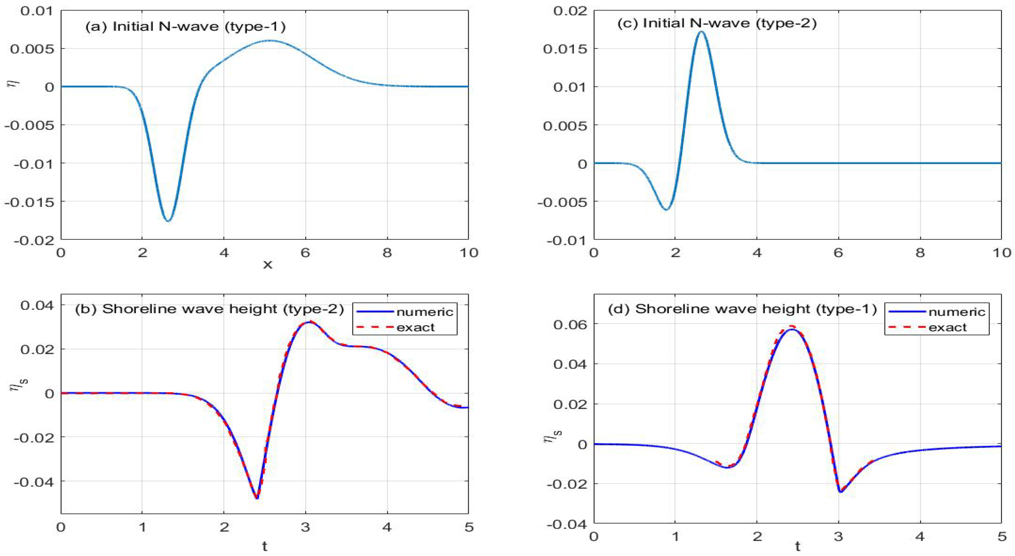
Validation of the model against the 1d solution of Carrier Greenspan 1958 has been conducted in [29,30]. As such, here we conducted validation of run-up and run-down using another analytical N-wave solutions, also from Carrier et al., (2003) [31]. Conducting this test case is important for a numerical scheme, to show its capability in predicting the moving shoreline. Here, we adopt the analytical solution of tsunami run-up and run-down wave of [31] for the analytical benchmarking. Following [31], in this subsection, the variables are dimensionless, with the acceleration of gravity is normalized to one. Moreover, since our scheme is 2-dimensional, we adopt this 1-d analytical solution and assume that it is homogeneous in the other direction. For numerical simulation, we adopt the leading depression wave shape given by
Two types of wave will be considered, those are
As described in [Carrier, 2003], wave type-1 is typically caused by a seismic fault dislocation, whereas wave type-2 is typically caused by submarine landslide. Both types of waves were plotted in Figure 5a,d.
First, we take the submarine landslide type of N-wave (31) as the initial wave with zero initial velocity, and let it propagates over a sloping bathymetry with
The sloping beach (34) connects the deepest part up to the dry area with a unit slope 1. The numerical scheme (11)–(14) is then implemented on a computational domain , using a set of parameter and (to fulfil stability condition), with normalized gravity . For the wet–dry procedure, we use a theshold number . From the simulation, we observed that the wave hit the beach starting with a wave of depression that causes run-down. The run-down goes further, and then the run-up starts. During the simulation the numerical shoreline wave height was recorded and plotted in Figure 5 along with the analytical shoreline. It is shown that our staggered conservative scheme could follow the analytical shoreline very well. A similar computation was conducted using initial profile of wave type-2, and the results are depicted in Figure 5c,d.
4. Numerical Model Benchmarking
In this section we performed the 2-d run-up test of a solitary hump that was first performed by Zelt, 1986 [21], and later by [12,32]. In this test case, the bathymetry is a flat bottom that is connected to a closed bay, as follows
with , . Here represents the offshore constant depth, and L the half-width of the bay. In Figure 6 the bay model (35) is plotted, together with the still water level m.
As a wave influx, we use the solitary hump profile with amplitude , using the explicit formula
There is no analytical solution for this case, here our numerical simulation is being tested against another shallow water codes of Özkan-Haller and Kirby, 1997 [23]. For our simulation, the bathymetry (35) is used with m, applied to a computational domain m, and the lateral dimension , with m. Hard wall boundaries were applied along both lateral boundaries, and . Parameters for simulation are , gravity acceleration m/s2, and the spatial grid size m, and s. For the wet–dry procedure, we use a threshold number of m.
The solitary wave (36) was introduced into the computational domain using the embedded method [22], as we mentioned earlier in Section 2.3. Implementation of this method requires that the computational domain was first extended from 0 m m to m m. This embedded influx was applied along m (shown in Figure 6 as the red dashed line) along with an absorbing boundary at m. In this way, we can obtain a transparent boundary at m, which allows the right running wave to enter the domain, while at the same time allowing the left running wave to leave the domain. This mechanism is important to ensure that the solitary hump that enters the bay, got reflected and propagated back to the left, leaving the domain via the left boundary m. In [23,32], this mechanism is referred to as the absorbing-generating offshore boundary.
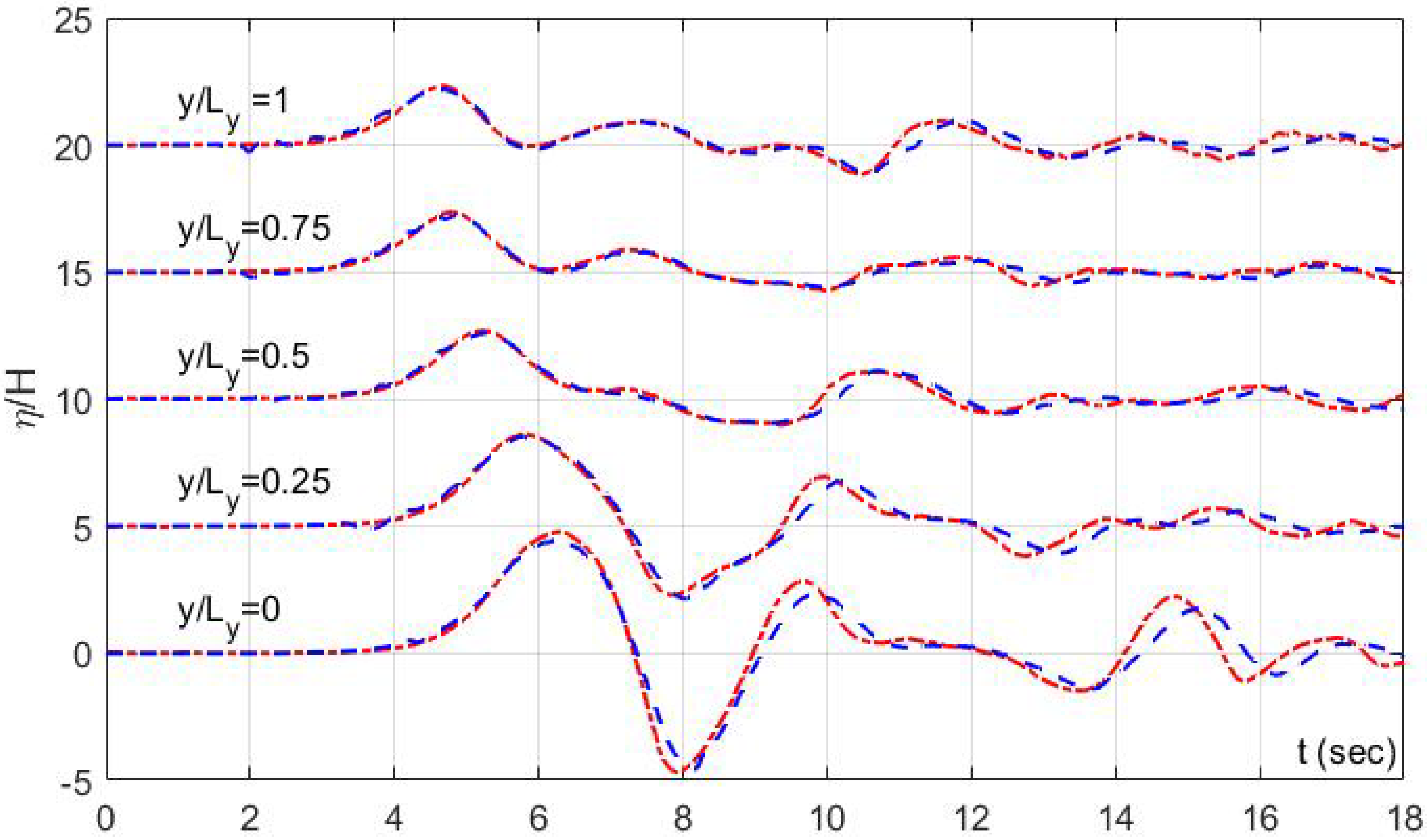
Simulation shows that the wave enters the domain and generates up and down motion, particularly in the closed bay area. The simulation results are compared with the numerical results by [23]. In Figure 7, time series of normalized waves run-up are compared at the middle of the bay , as well as at several cross-sections . It is shown that the highest run-up and run-down were achieved in the middle of the bay, and a little less were achieved along the other cross-sections, with the least run-up being reached along the lateral borders at . The numerical results in all five cross-sections show a good resemblance to the numerical results. Further comparison was made with the maximum wave height along the shoreline on the bay beach, see Figure 6. As shown in that figure, the calculated maximum run-up and minimum run-down, are in satisfactory agreement with the maximum wave height found by [23].
5. Laboratory Benchmarking
In this section we performed laboratory benchmark tests as recommended for by NOAA [20], which are (1) a solitary wave run-up on a conical island, and (2) wave run-up onto a complex bathymetry. This solitary wave run-up on a conical island is favorable test case often performed by tsunami modelers, see for example [32,33,34]. In addition, the laboratory data set of solitary wave run-up and run-down by Synolakis, 1987 [35] is normally used to validate the accuracy of a numerical model in predicting a solitary wave run-up on a sloping beach. However, this has been done by Erwina et al., 2019 [29] using the 1d version of this MCS-2d scheme. It has been shown that the run-up of solitary wave confirms the experimental data for a wide range of wave heights of and , i.e., non-breaking and breaking case, respectively. So, here we go straight to the test case of a solitary wave run-up on a conical island.
5.1. A Solitary Wave Run-Up on a Conical Island
This simulation is based on a laboratory experiment performed at the Coastal Engineering Research Center, Vicksburg, Mississippi, which is motivated by the 1992 Flores Island tsunami. The experiment was conducted in a 30-m-wide, 25-m-long, and 60-cm-deep wave basin with a conical island in the center. The slope of the island is 1:4 and the water depth is m. This experiment simulates the interaction of solitary wave around conical island. Detail of the experiment can be found in [25].
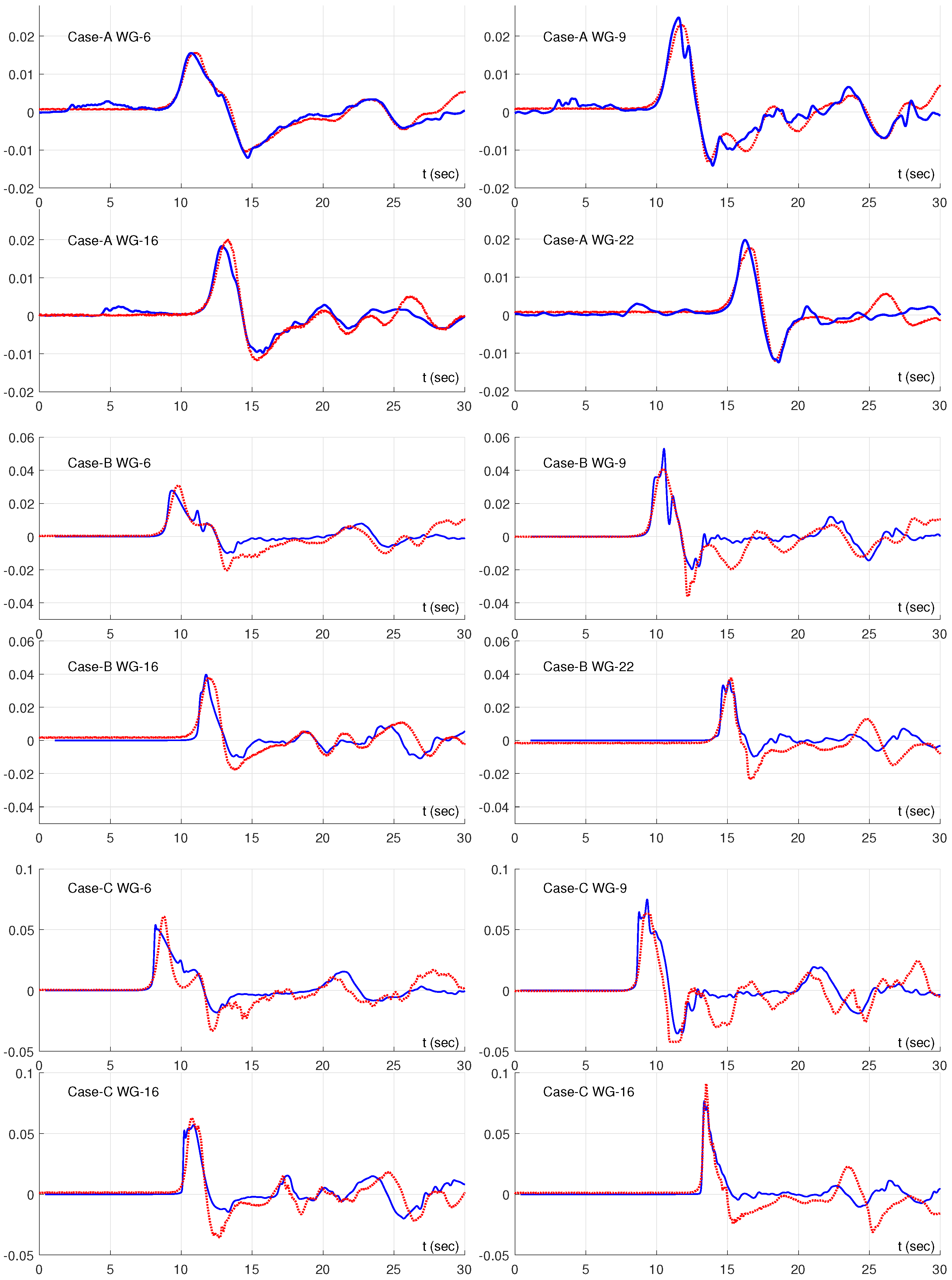
Numerical simulation was performed using m and s, and the threshold number m. Here we conduct a simulation, in which the initial soliton of a certain amplitude enters the numerical domain from the left boundary. The surface elevation was recorded at four wave gauge locations WG6, WG9, WG16, and WG22, as shown in Figure 8. Three wave gauges WG9, WG16, WG22 were located at the initial shoreline surrounding the island, whereas WG6 is located near the front face of the island.
The propagation of soliton at subsequent times are shown in Figure 9. When the soliton reaches the island, it moves around the perimeter of the island and then moving forward leaving the island. Three cases of solitary wave amplitudes were simulated; case A (), case B (), case C (). During all simulations, wave signal at several wave gauges WG6, WG9, WG16, WG22 were recorded for comparison purposes, and the results are shown in Figure 9. It is shown that the leading wave run-up can be captured well with our numerical scheme. However, for the secondary depression wave, our numerical result shows less of a depression. But this result is consistent with other run-up model tests [33,36].
Moreover, the calculated maximum run-up around the conical island has also been recorded. This maximum run-up measures the highest vertical extend that can be reached by the wave influx. The maximum run-up from numerical calculation is compared with the laboratory data in Figure 10. The numerical predictions are good around the front of the island, and this holds for all three cases. However, around the back of the island, there is a slight under prediction that could be due to the absence of bottom friction in the numerical runs.
5.2. Wave Run-Up onto a Complex Beach (Monai Valley)
In this section, we do another benchmark test simulation based on experiment [28]. The experiment was conducted at Central Research Institute for Electric Power Industry (CRIEPI), Abiko, Japan. The aim of this experiment is to reproduce the 1993 Hokkaido-Nansei-Oki (HNO) tsunami. The tsunami that struck Okushiri Island, Japan, reached an extreme height of 30 m in a small valley near the Monai village. The laboratory model was built to represent the actual bathymetry of Monai Valley, and is arranged on a scale of 1:400. This is one of the important benchmark tests for tsunami numerical models recommended by NOAA, so all data are disclosed by NOAA.
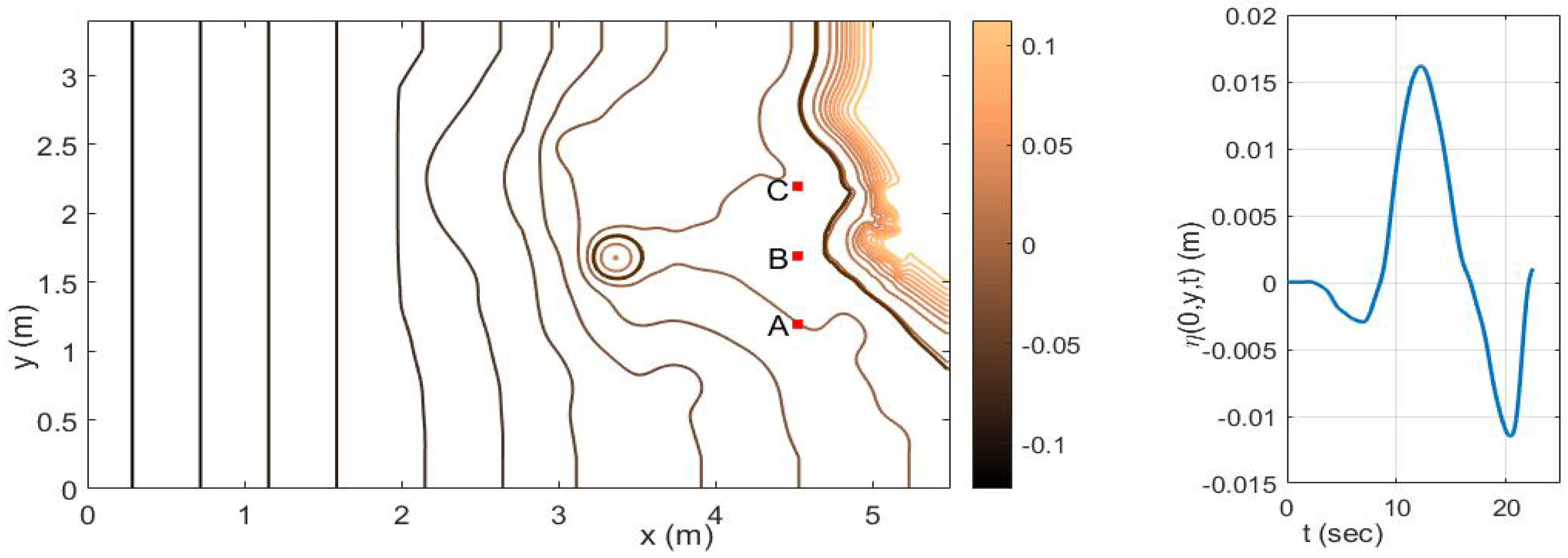
To test our model, a numerical simulation was performed on a m computational domain with m and s, and a threshold water depth of m. For bathymetry, we use the Monai Valley model profile as shown in Figure 11 (left). The lead-depression wave, with height of cm and a crest of cm, shown in Figure 11 (right) is used for the left wave influx . This wave influx was introduced into the domain using the embedded method [22].
As time progresses, the wave enters the domain and propagates towards Monai beach, see Figure 12. The wave reaches the beach at s and maximum run-up occurs at s near Monai Valley. Closer observation, Figure 13 (left) shows the maximum inundated area obtained from numeric, whereas Figure 13 (right) is form the experiment. As observed, the area of inundation is very well captured by the simulation.
Figure 14 presents the recorded wave signals at three observational points , and . For all comparisons, the main wave is predicted very well by the numerical model. Some discrepancy is observed after 30 s simulation time, which is likely because of reflection from the computational boundary.
6. Conclusions
The new numerical implementation of the momentum conserving staggered grid MCS-2d scheme was discussed in this paper. The scheme itself is explicit, non-dissipative and relatively easy to implement. Validation with two types of analytical solutions, as well as the case of a solitary wave run-up in a closed bay, produced favourable results. In addition, two laboratory benchmark tests, as recommended by NOAA, were given good agreement. Apart from the correct implementation of the wet–dry procedure, and the transparent offshore boundary condition, in essence, no special treatment was required for all simulations presented in this paper. All these observations have shown the robustness and ability of the MCS-2d scheme to predict accurate results for various problems. It can be concluded that the numerical model MCS-2d is appropriate for further study of the surf zone phenomena.
Abbreviations
The following abbreviations are used in this manuscript:
| MCS-2d | 2-dimensional Momentum Conserving Staggered grid |
| 2d-SWE | 2-dimensional Shallow Water Equation |
Author Contributions
Conceptualization, S.R.P., D.A.; methodology, N.E., S.R.P.; software, S.R.P., D.A.; validation, N.E., S.R.P., D.A., and T.N.; formal analysis, S.R.P., D.A.; writing—original draft preparation, N.E., S.R.P.; writing—review and editing, S.R.P., D.A.; funding acquisition, S.R.P. All authors have read and agreed to the published version of the manuscript.
Funding
This research was funded by Institut Teknologi Bandung research grant number 2S/I1.C01/PL/2020 and Indonesian Research Grant number 2/E1/KP.PTNBH/2020.
Conflicts of Interest
The authors declare no conflict of interest.
References
- Kounadis, G.; Dougalis, V.A. Galerkin finite element methods for the Shallow Water equations over variable bottom. J. Comput. Appl. Math. 2020, 373, 112315. [Google Scholar] [CrossRef] [Green Version]
- Li, P.; Don, W.S.; Gao, Z. High order well-balanced finite difference WENO interpolation-based schemes for shallow water equations. Comput. Fluids 2020, 201, 104476. [Google Scholar] [CrossRef]
- Khakimzyanov, G.; Dutykh, D.; Mitsotakis, D.; Shokina, N.Y. Numerical simulation of conservation laws with moving grid nodes: Application to tsunami wave modelling. Geosciences 2019, 9, 197. [Google Scholar] [CrossRef] [Green Version]
- Alcrudo, F.; Garcia-Navarro, P. A high-resolution Godunov-type scheme in finite volumes for the 2D shallow-water equations. Int. J. Numer. Methods Fluids 1993, 16, 489–505. [Google Scholar] [CrossRef]
- Anastasiou, K.; Chan, C. Solution of the 2D shallow water equations using the finite volume method on unstructured triangular meshes. Int. J. Numer. Methods Fluids 1997, 24, 1225–1245. [Google Scholar] [CrossRef]
- Sleigh, P.; Gaskell, P.; Berzins, M.; Wright, N. An unstructured finite-volume algorithm for predicting flow in rivers and estuaries. Comput. Fluids 1998, 27, 479–508. [Google Scholar] [CrossRef]
- Guillou, S.; Nguyen, K. An improved technique for solving two-dimensional shallow water problems. Int. J. Numer. Methods Fluids 1999, 29, 465–483. [Google Scholar] [CrossRef]
- Begnudelli, L.; Sanders, B.F. Unstructured grid finite-volume algorithm for shallow-water flow and scalar transport with wetting and drying. J. Hydraul. Eng. 2006, 132, 371–384. [Google Scholar] [CrossRef]
- Marche, F.; Bonneton, P.; Fabrie, P.; Seguin, N. Evaluation of well-balanced bore-capturing schemes for 2D wetting and drying processes. Int. J. Numer. Methods Fluids 2007, 53, 867–894. [Google Scholar] [CrossRef]
- Guan, M.; Wright, N.; Sleigh, P. A robust 2D shallow water model for solving flow over complex topography using homogenous flux method. Int. J. Numer. Methods Fluids 2013, 73, 225–249. [Google Scholar] [CrossRef]
- Toro, E.F. Riemann Solvers and Numerical Methods for Fluid Dynamics: A Practical Introduction; Springer: Berlin/Heidelberg, Germany, 2013. [Google Scholar]
- Brocchini, M.; Dodd, N. Nonlinear shallow water equation modeling for coastal engineering. J. Waterw. Port Coast. Ocean Eng. 2008, 134, 104–120. [Google Scholar] [CrossRef]
- Kärnä, T.; De Brye, B.; Gourgue, O.; Lambrechts, J.; Comblen, R.; Legat, V.; Deleersnijder, E. A fully implicit wetting–drying method for DG-FEM shallow water models, with an application to the Scheldt Estuary. Comput. Methods Appl. Mech. Eng. 2011, 200, 509–524. [Google Scholar] [CrossRef]
- Lu, X.; Mao, B.; Zhang, X.; Ren, S. Well-balanced and shock-capturing solving of 3D shallow-water equations involving rapid wetting and drying with a local 2D transition approach. Comput. Methods Appl. Mech. Eng. 2020, 364, 112897. [Google Scholar] [CrossRef]
- Madsen, P.A.; Sørensen, O.; Schäffer, H. Surf zone dynamics simulated by a Boussinesq type model. Part I. Model description and cross-shore motion of regular waves. Coast. Eng. 1997, 32, 255–287. [Google Scholar] [CrossRef]
- Medeiros, S.C.; Hagen, S.C. Review of wetting and drying algorithms for numerical tidal flow models. Int. J. Numer. Methods Fluids 2013, 71, 473–487. [Google Scholar] [CrossRef]
- Stelling, G.S.; Duinmeijer, S.A. A staggered conservative scheme for every Froude number in rapidly varied shallow water flows. Int. J. Numer. Methods Fluids 2003, 43, 1329–1354. [Google Scholar] [CrossRef]
- Arakawa, A. Computational design for long-term numerical integration of the equations of fluid motion: Two-dimensional incompressible flow. Part I. J. Comput. Phys. 1997, 135, 103–114. [Google Scholar] [CrossRef] [Green Version]
- Pudjaprasetya, S.; Magdalena, I. Momentum conservative scheme for dam break and wave run up simulations. East Asian J. Appl. Math 2014, 4, 152–165. [Google Scholar] [CrossRef]
- Synolakis, C. Standards, Criteria, and Procedures for NOAA Evaluation of Tsunami Numerical Models; NOAA: Washington, DC, USA, 2007. [Google Scholar]
- Zelt, J.A. Tsunamis: The Response of Harbours with Sloping Boundaries to Long Wave Excitation. Ph.D. Thesis, California Institute of Technology, Pasadena, CA, USA, 1986. [Google Scholar]
- Liam, L.S.; Adytia, D.; Van Groesen, E. Embedded wave generation for dispersive surface wave models. Ocean Eng. 2014, 80, 73–83. [Google Scholar] [CrossRef] [Green Version]
- Özkan-Haller, H.T.; Kirby, J.T. A Fourier-Chebyshev collocation method for the shallow water equations including shoreline runup. Appl. Ocean Res. 1997, 19, 21–34. [Google Scholar]
- Thacker, W.C. Some exact solutions to the nonlinear shallow-water wave equations. J. Fluid Mech. 1981, 107, 499–508. [Google Scholar] [CrossRef]
- Briggs, M.J.; Synolakis, C.E.; Harkins, G.S.; Green, D.R. Laboratory experiments of tsunami runup on a circular island. Pure Appl. Geophys. 1995, 144, 569–593. [Google Scholar] [CrossRef]
- Stelling, G.S.; Wiersma, A.; Willemse, J. Practical aspects of accurate tidal computations. J. Hydraul. Eng. 1986, 112, 802–816. [Google Scholar] [CrossRef]
- Balzano, A. Evaluation of methods for numerical simulation of wetting and drying in shallow water flow models. Coast. Eng. 1998, 34, 83–107. [Google Scholar] [CrossRef]
- Liu, P.; Yeh, H.; Synolakis, C. Advanced numerical models for simulating tsunami waves and runup. Adv. Coast. Ocean Eng. 2008, 10, 250. [Google Scholar]
- Erwina, N.; Pudjaprasetya, S.R.; Soeharyadi, Y. The momentum conservative scheme for wave run-up on a sloping beach. Adv. App. Fluid Mech. 2018, 21, 493–510. [Google Scholar] [CrossRef]
- Ginting, M.; Pudjaprasetya, S.; Adytia, D. Two layers non-hydrostatic scheme for simulations of wave runup. J. Earthq. Tsunami 2019, 13, 1941004. [Google Scholar] [CrossRef]
- Carrier, G.F.; Wu, T.T.; Yeh, H. Tsunami run-up and draw-down on a plane beach. J. Fluid Mech. 2003, 475, 79. [Google Scholar] [CrossRef]
- Hubbard, M.E.; Dodd, N. A 2D numerical model of wave run-up and overtopping. Coast. Eng. 2002, 47, 1–26. [Google Scholar] [CrossRef]
- Liu, P.L.F.; Cho, Y.S.; Briggs, M.J.; Kanoglu, U.; Synolakis, C.E. Runup of solitary waves on a circular island. J. Fluid Mech. 1995, 302, 259–285. [Google Scholar] [CrossRef]
- Wei, Y.; Mao, X.Z.; Cheung, K.F. Well-balanced finite-volume model for long-wave runup. J. Waterw. Port Coast. Ocean Eng. 2006, 132, 114–124. [Google Scholar] [CrossRef] [Green Version]
- Synolakis, C.E. The runup of solitary waves. J. Fluid Mech. 1987, 185, 523–545. [Google Scholar] [CrossRef]
- Lynett, P.J.; Wu, T.R.; Liu, P.L.F. Modeling wave runup with depth-integrated equations. Coast. Eng. 2002, 46, 89–107. [Google Scholar] [CrossRef]
Sample Availability: Samples of the compounds ... are available from the authors. |
Figure 1.
(Left) Sketch of the fluid domain and notations. (Right) Arakawa-C grid with illustrations for mass and momentum cells.
Figure 1.
(Left) Sketch of the fluid domain and notations. (Right) Arakawa-C grid with illustrations for mass and momentum cells.

Figure 2.
Centerline of planar surface profile from numerical as well as the analytical at subsequent times , with period s.
Figure 2.
Centerline of planar surface profile from numerical as well as the analytical at subsequent times , with period s.

Figure 3.
Surface oscillation at subsequent times , with period s.

Figure 4.
(left) Surface profile in the parabolic flood wave test case, (right) centerline surface at time , at which the maximum wave height has reduced from 1 m to m.
Figure 4.
(left) Surface profile in the parabolic flood wave test case, (right) centerline surface at time , at which the maximum wave height has reduced from 1 m to m.

Figure 5.
(Top left-right) The initial N-wave of type-1 and type-2, (bottom left-right) shoreline wave height of type-1 and type-2. The analytical shorelines are digitized from [31].
Figure 5.
(Top left-right) The initial N-wave of type-1 and type-2, (bottom left-right) shoreline wave height of type-1 and type-2. The analytical shorelines are digitized from [31].

Figure 6.
(Left) Bathymetry of a sloping bay and the still water level. The red line indicates the embedded influx line. (Right) Maximum run-up and run-down at the beach calculated using MCS-2d scheme in comparison with those of Özkan and Kirby, 1997 [23].
Figure 6.
(Left) Bathymetry of a sloping bay and the still water level. The red line indicates the embedded influx line. (Right) Maximum run-up and run-down at the beach calculated using MCS-2d scheme in comparison with those of Özkan and Kirby, 1997 [23].

Figure 7.
Wave signal at several cross-sections , the numerical MCS-2d scheme (blue) versus another SWE solver by Özkan-Haller and Kirby, 1997 [23] (red).
Figure 7.
Wave signal at several cross-sections , the numerical MCS-2d scheme (blue) versus another SWE solver by Özkan-Haller and Kirby, 1997 [23] (red).

Figure 8.
The location of wave gauges.

Figure 9.
Surface elevation at WG-6, WG-9, WG-16, dan WG-22. Numerical results (blue solid line) and experimental data (red dotted line). (Top) Case A , (Middle) Case B , (Bottom) Case C .
Figure 9.
Surface elevation at WG-6, WG-9, WG-16, dan WG-22. Numerical results (blue solid line) and experimental data (red dotted line). (Top) Case A , (Middle) Case B , (Bottom) Case C .

Figure 10.
Maximum inundation area of numerical result (blue lines) and experiment (red stars). The solid brown lines represent the initial shoreline. From left to right, case A, case B and case C.
Figure 10.
Maximum inundation area of numerical result (blue lines) and experiment (red stars). The solid brown lines represent the initial shoreline. From left to right, case A, case B and case C.

Figure 11.
(Left) Topographic profile and contour plot of Monai Valley. Point A, B, and C are the observation points. (Right) Incident waves profile
Figure 11.
(Left) Topographic profile and contour plot of Monai Valley. Point A, B, and C are the observation points. (Right) Incident waves profile

Figure 12.
Shoreline at t = 0 s, 14 s, 15 s, 15,7 s, 16,3 s, 17 s. The contour of water level (blue line), shoreline (bold blue line), beach (brown line), and initial shoreline (bold brown line).
Figure 12.
Shoreline at t = 0 s, 14 s, 15 s, 15,7 s, 16,3 s, 17 s. The contour of water level (blue line), shoreline (bold blue line), beach (brown line), and initial shoreline (bold brown line).

Figure 13.
Shoreline from simulation (blue solid line) in (a) and shoreline from experiment by Liu et al., 2008 (yellow dash line) in (b) when maximum run-up occurs.
Figure 13.
Shoreline from simulation (blue solid line) in (a) and shoreline from experiment by Liu et al., 2008 (yellow dash line) in (b) when maximum run-up occurs.

Figure 14.
Numerical result (blue) and experimental data (red) at location A (top), B (middle) dan C (bottom).
Figure 14.
Numerical result (blue) and experimental data (red) at location A (top), B (middle) dan C (bottom).

© 2020 by the authors. Licensee MDPI, Basel, Switzerland. This article is an open access article distributed under the terms and conditions of the Creative Commons Attribution (CC BY) license (http://creativecommons.org/licenses/by/4.0/).
Share and Cite
MDPI and ACS Style
Erwina, N.; Adytia, D.; Pudjaprasetya, S.R.; Nuryaman, T. Staggered Conservative Scheme for 2-Dimensional Shallow Water Flows. Fluids 2020, 5, 149. https://0-doi-org.brum.beds.ac.uk/10.3390/fluids5030149
AMA Style
Erwina N, Adytia D, Pudjaprasetya SR, Nuryaman T. Staggered Conservative Scheme for 2-Dimensional Shallow Water Flows. Fluids. 2020; 5(3):149. https://0-doi-org.brum.beds.ac.uk/10.3390/fluids5030149
Chicago/Turabian StyleErwina, Novry, Didit Adytia, Sri Redjeki Pudjaprasetya, and Toni Nuryaman. 2020. "Staggered Conservative Scheme for 2-Dimensional Shallow Water Flows" Fluids 5, no. 3: 149. https://0-doi-org.brum.beds.ac.uk/10.3390/fluids5030149