Analysis of the Aerodynamics in the Heating Section of an Anode Baking Furnace Using Non-Linear Finite Element Simulations

Abstract

The emissions from the industrial furnaces impact the environment. Among the various factories, those having anode baking furnaces are working on reducing the pollutant emissions. The aerodynamics in the furnace influences the emissions due to the high dependence of combustion and radiation phenomena on the mixing characteristics. Therefore, this paper aims to establish the numerical simulation results for the three-dimensional turbulent flow in a single section of an anode baking furnace with a high rate of fuel injection. The stabilized non-linear finite element approach on the Reynolds-averaged Navier-Stokes (RANS) equation is used with COMSOLMultiphysics. The turbulent viscosity ratio is highly sensitive to the mesh for the standard k-$ϵ$ model. The requirements of the Cartesian and refined mesh near the jet development region is explained. The comparison of meshes generated by two meshing tools namely cfMesh and COMSOL Multiphysics default Mesher is carried out. The high numerical diffusion in the flow models due to the coarser mesh leads to convergence but deficit the precision in the results. This paper shows that the mesh generated by cfMesh with flow aligned refinement combined with the non-linear finite element solver in COMSOL Multiphysics proves to provide accurate results of turbulent quantities.

1. Introduction

The combustion process is the most important process to extract energy from fossil fuels. The majority of the usage of burning fossil fuels is carried out in industries [1]. The combustion of gaseous hydrocarbon fuels in industries that manufacture raw materials such as steel, glass, cement, and so forth. is still indispensable due to high energy density levels. The byproduct of the combustion of fossil fuels is the pollutant gases that have a significant impact on environment. Due to the consequential amount of pollutant formation from industries, the governments provide regulations on the allowed pollutant quantities that can be emitted. There have been several studies that propose techniques to curb pollutant gases at the source [2,3]. This encourages industries to make the combustion process more efficient by reducing the formation of pollutant gases, reducing the usage of fuel, and optimizing energy consumption. The traditional trial and error approach is limited due to the difficulty of handling the high temperature. Moreover, the resource requirements for such trials can be high leading to a longer time needed for the successful attempt. The numerical modeling of the process in such applications can be of advantage to achieve an efficient process.

There are numerous industries that are based on the combustion of fossil fuels as the energy source. Aluminium, for example, is extracted from the Bauxite using the Hall-Héroult process. The Hall-Héroult process is the electrolysis process in which anodes wear out continuously. Thus, the anodes need to be regularly replaced. The carbon anodes used in the extraction process should have properties such as high density, conductivity, mechanical strength, and low reactivity in the process. The anodes need to be baked before using in the Hall-Héroult to gain these properties. This gives rise to an auxiliary industry in which anodes are baked. The anode baking process has gained attention due to its high costs and energy demand. 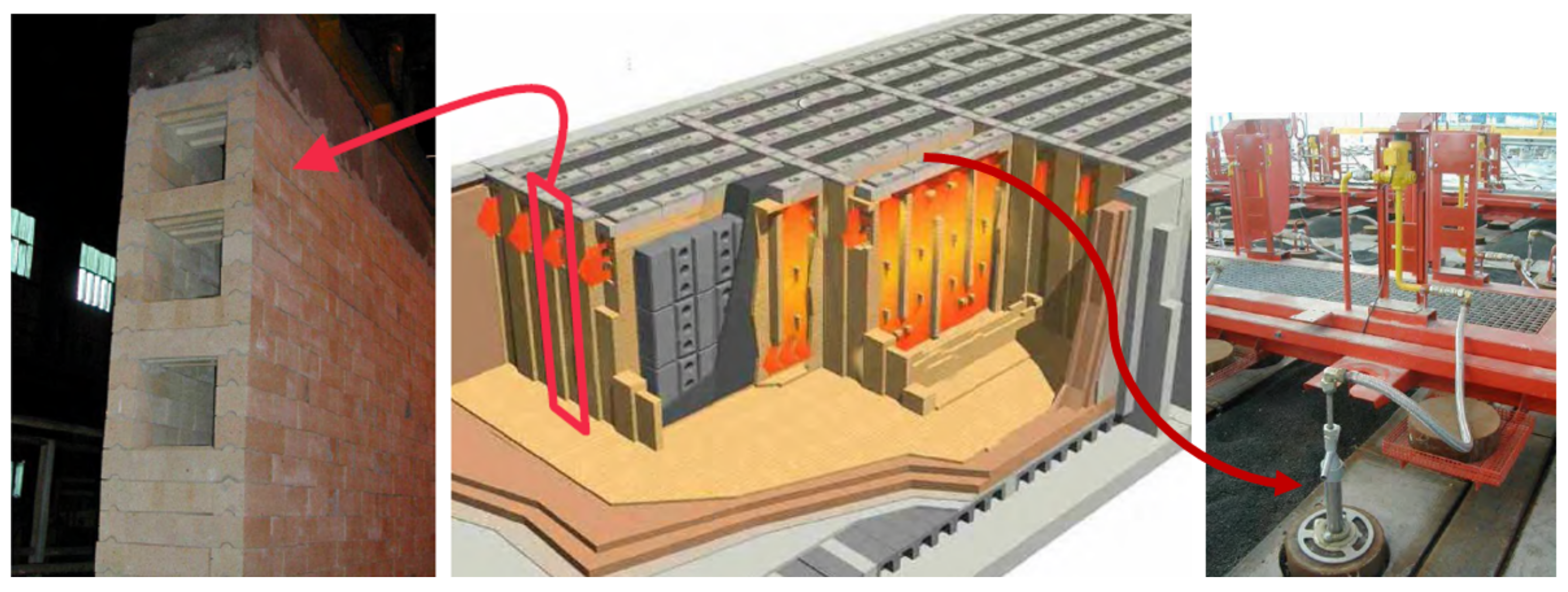Figure 1 shows a schematic representation of a horizontal ring anode baking furnace. The furnace consists of the flue and the pits in which raw anodes are loaded. As shown in Figure 1, the air flows in the horizontal direction through the flue. The left picture from Figure 1 shows the channel through which gas flows from one section to another. The combustion process occurs in the flue when the injected fuel reacts with air flowing through the channel. The fuel is injected from the top holes. The heat generated during the combustion process is conducted through the walls and packing material to the anodes.

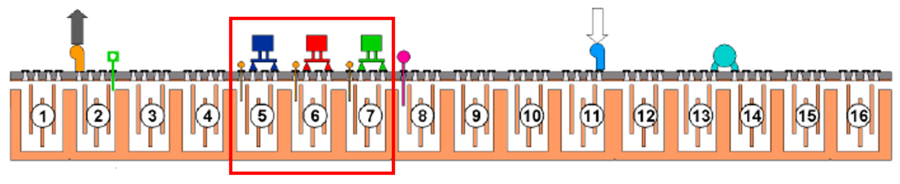
It is important to understand the overall process to define a model. The process in the anode baking furnace is such that there is a continuous exchange of heat either from the hot gases to the wall or from the walls to the gases. Based on the transfer of heat, the anode baking furnace is divided into zones such as preheating, heating, blowing, and cooling zone. Each zone consists of three or four sections. Figure 2 presents the schematic representation of the various zones in the anode baking furnace. In the preheating zone, the raw anodes are loaded in the pits. Whereas, in the adjacent flue, the heated gas exiting from the heating section is circulating. The transfer of heat in this section occurs from the flue to the anodes. The temperature of the anodes is increased to approximately 550 ${}^{\circ }$C in this section. In the heating section, the fuel (natural gas) is injected from the top. Figure 2 shows a total of three ramps (one for each section) with two burners on each ramp. In the heating section, the combustion of natural gas is carried out due to the contact with air at ignition temperature. The transfer of heat occurs from the flue gas to the anodes. As a result, the temperature of anodes further increases to approximately 1100 ${}^{\circ }$C. In the third zone that is, blowing zone, the air is injected using the blowing ramp. In this zone, the anodes are already heated. Therefore, the transfer of heat occurs from the anodes to the cold air. This results in an increase of gas temperature to 1150 ${}^{\circ }$C. The last zone is the cooling zone in which the anodes are further cooled using external fans so as to post-process. Therefore, to study NOx emissions, only the heating section of the furnace is important.

The modeling of anode baking furnace has been developed since 1980’s [4]. The early models form the basis of the anode baking furnace modeling developed further. The literature available on the modeling suggests that there is a wider scope of improvement in the anode baking process with respect to a variety of goals. Some of the examples are optimizing energy consumption, reducing soot and NOx formation, increasing the anode quality, and improving the lifespan of the refractory. The modeling approach developed by Gosselin et.al. [5] focuses on the choice of combustion model for anode baking furnace. They provide the sensitivity of maximum temperature computed by three combustion model approaches namely, eddy dissipation model, mixture fraction/pdf model, and hot jet approach. The study provides insights on the advantage of the mixture fraction/pdf combustion model to predict accurate maximum temperature. The effect of radiation coupling is also essential for computing the accurate maximum temperature. The study carried out by Tajik et. al. [6] provides results for combinations of turbulent flow models, combustion models, and radiation models. The results are extended for the anode baking furnace model. They conclude that the realizable k-$ϵ$ model, mixture fraction/pdf model, and discrete ordinate-WSGGM (weighted-sum-of-gray-gas-modeling) are the appropriate models. Further work by Tajik et. al. [7] on the calculations of NOx emissions by studying the effect of re-circulation of exhaust gases and diluting the inlet oxygen concentration at elevated temperature shows the lowering of emissions. Another modeling by Bessen et. al. [8] studies the different parameters of the burner designs for high-velocity fuel injection to predict NOx formation.

Among various industries, Aluchemie BV Rotterdam has anode baking furnaces in The Netherlands. Aluchemie is working on reducing the NOx emissions from the furnace to meet the stringent requirements by local authorities. The furnace geometry of Aluchemie is slightly different from the other furnaces presented in the literature. In the models by Gosselin et.al. [5] and by Tajik et.al [6], the fuel pipes are inserted deeper into the flue and have a lower fuel injection velocity than is the case in this paper. In the Aluchemie furnace, the fuel pipe from the burner does not penetrate directly into the furnace. In practice, such penetration in the furnace poses the problem of higher waring of fuel pipe. There have been various studies that show the impact of geometry modification on the flow dynamics in the furnace [6]. The modeling for the geometry specific to the anode baking furnace of Aluchemie is required. Therefore, this work is dedicated to the development of the anode baking furnace of Aluchemie. The aerodynamics forms the basis of the modeling in the anode baking process. Since no such modeling was carried out in Aluchemie before, the model is developed from scratch. Therefore, the model discussed in this paper is based on the Reynolds-averaged Navier-Stokes (RANS) equations for modeling the non-reactive turbulent flow. This avoids going over the more complicated Large Eddy Simulation (LES) or Direct Numerical Simulation (DNS) models.

The goal of this work is to provide suitable modeling techniques to reduce NOx emissions from the anode baking furnace. It should be noted that NOx is not generated in all sections. The temperature in the preheating section is not high enough to form NOx and therefore, the NOx formation in the preheating section remains negligible. The temperature in the flue gas in the heating section is more than 1300 ${}^{\circ }$C and provides suitable conditions for the generation of NOx. Therefore, for studying the NOx formation in the anode baking furnace, it is important to focus on the aerodynamics in the heating sections.

In this paper, a detailed analysis of the turbulent flow modeling in a single heating section of the flue is carried out. The COMSOL Multiphysics software with version 5.4 is used for the modeling. The COMSOL Multiphysics is a finite element based solver and uses the Newton method with a coupled pressure-velocity approach [9]. The software has been proven to provide excellent coupling between different physical phenomena and is easily accessible for academia. With this paper, we aim to provide converged simulation results of the turbulent flow in the heating section of the anode baking furnace. Moreover, the role of the Newton solver for coupled pressure-velocity approach on the Cartesian mesh of realistic geometry is elaborated.

The anode baking process is a multi-physical phenomenon. Understanding the aerodynamics in the furnace is crucial for modeling the NOx formation due to the high dependence of combustion and radiation on the flow. This motivates us to describe the flow simulation results in detail. The accuracy of any numerical model depends significantly on the discretization of the equations under investigation. The finite element discretization used in the current work is further dependent on the type of mesh. Due to the complexity of anode baking furnace geometry, it is not straightforward to obtain the desired mesh. Therefore, the analysis of the results with varying meshes is important. In this work, the results with the two meshing tools namely, cfMesh version 3.2 and COMSOL default mesher are compared using the standard k-$ϵ$ model. Moreover, the sensitivity of the solution to the refinement in the region of jet development is studied. The effect on the results due to the higher numerical diffusion of coarser mesh is explained. The study is extended to the less diffusive realizable k-$ϵ$ model. The effect of various parameters on the convergence behavior of the realizable k-$ϵ$ model is described to provide guidelines on getting the converged solution. The paper describes the role of the Cartesian and flow aligned mesh to improve the flow description as well as their effect on the convergence behavior.

In the next section, the geometry definition, non-isothermal cross-flow conditions, mesh generation techniques, governing equations, finite elements discretization, and the pseudo-time stepping solver within non-linear and linear equations is described. In the results section, the baseline model is discussed followed by a comparison with various meshes. In the next section, the challenges in the convergence of the realizble k-$ϵ$ model are discussed.

2. Model Description

2.1. Geometry Definition

The source of the NOx formation in the anode baking furnace is in the heating sections. In other sections of the furnace, high-temperature zones required for the formation of NOx are not observed. Therefore, the model is confined to the heating section of the furnace in this study. The 3D geometry of the model is as shown in Figure 3. To study the effect of the design parameters, there have various flue designs modeled in the published literature [6,8]. The geometry of the model studied in this paper is based on the existing furnace design from Aluchemie factory. The length of the outlet pipe is such that the backflow is suppressed and uniform pressure distribution is ensured at the outlet. The focus of the paper is to understand the importance of accurate computation of the flow of the gas in the furnace. Therefore, the geometry consists of only the flue domain. The geometry consists of three air inlet pipes, three outlet pipes, and two fuel inlets as shown in Figure 3. The burner has been simplified to a simple pipe with a length of 1.1 m and a diameter of 0.009 m. The typical bypass dimensions at top and bottom are 0.084 [m] in y-direction. The rectangular obstacles with smoothed corners are the tie-bricks required for the structural strength of the furnace and also aids in providing turbulence. The three baffles direct the flow in the desired direction. The symmetry in the flue wall is assumed. Therefore, the depth of the furnace is halved to 0.27 m. The geometry files are available for download in STL format so as to provide open-domain benchmark configuration with this link https://0-doi-org.brum.beds.ac.uk/10.4121/13522763.v2.

2.2. Non-Isothermal Fuel Jets in Cross-Flow

The overall anode baking furnace modeling consists of various phases namely a gas phase on the flue side and a solid phase on the wall, anodes, and packing coke. In this paper, the focus is only on the gas phase in the furnace. The flow in the heating section of an anode baking furnace is characterized by the air from the side inlets and fuel flow from the top inlets. The outlet is on the other side in the perpendicular direction to the fuel inlet as shown in Figure 3. The air and fuel interact in a cross-flow manner. Apart from providing structural strength, the tie-bricks also aids in the aerodynamics of the flow. The small openings at the top of the furnace are required to avoid the dead flow and the associated hot spots at the corners. The presence of baffles directs the flow in the U shape providing maximum mixing of the air and the fuel and assure overall heating of the wall. Aluchemie furnaces have by-passes to avoid hot spots in the dead zones and thereby, ensuring safety in the furnace.

The Reynolds number at the fuel inlet and air inlet are around 13,000 and 8500, respectively. The Reynolds number is calculated based on Equation (1). The parameters values are mentioned in

Table 1. Inflow conditions at fuel and air inlets.

Property	Symbol	Air Inlet	Fuel Inlets	Initial Condition
Velocity [m/s]	U${}_{ref}$	1.45	74	0
Temperature [K]	T	1050	300	300
Re [-]	Re	8500	13,000	-
Turbulent length scale [m]	L${}_T$	0.01	0.01	-
Turbulent intensity [%]	I${}_T$	0.05	0.05	-

and

Table 2. Physical properties of the gas.

Physical Property	Symbol	Values
Specific heat capacity [J/(kg×K)]	Cp	1004.5
Ratio of specific heats [-]	$\gamma$	1.4
Prandtl number [-]	Pr	0.73
Molecular viscosity [kg/(m×s)]	$\mu$	1.8×10${}^{-5}$

. The diameter for the air and fuel inlets are mentioned in Figure 3. Table 1 provides the fuel inlet and air inlet boundary conditions. Due to the high velocity of the fuel, the jet is expected to penetrate deeper and provide higher turbulent mixing. The presence of tie-bricks generates backflow due to the adverse pressure gradient. The effects of the backflow are highly dependent on the velocity of the jet.

$$Re=\frac{\rho U_{ref}D}{\mu }.$$

(1)

The air and fuel streams are injected at different temperatures. The effect of temperature variations on the flow is considered by taking into account the variation of density with respect to the temperature. The physical properties of the gas in the flue are as mentioned in Table 2.

2.3. Mesh Generation

The outcome of the numerical model of flow computations is highly influenced by the mesh. The burners used in the Aluchemie operates at high velocity of fuel injection. The computations of higher velocity regime demands for the Cartesian and flow aligned mesh. As will be discussed later, non-linear finite element solver is utilized in the present study which further requires a better quality mesh.

The requirement of the Cartesian mesh is elaborated in the previous work [10]. The detailed analysis shows that the differences in the results obtained by two simulation environments is due to the size and structure of the mesh. The presence of tie-bricks, by passes and baffles impose challenges to obtain a hexahedral mesh. The dimensions of the geometrical entities varies from mm to m in the flue domain of the anode baking furnace. Moreover, the turbulent flow in the furnace is such that a refined mesh is required in the regions of interaction of air and fuel. To generate such mesh with the available meshing techniques in COMSOL Multiphysics is difficult. In the results section, the inefficacy of the mesh generated with the COMSOL software for the anode baking application is described. Therefore, advanced software dedicated for the mesh generation is required. In this study, a new meshing technique is developed to construct a well-structured Cartesian mesh with cfMesh software version 3.2.1.

cfMesh is a collection of mesh generation tools distributed as a library [11]. This library is designed to provide customizable meshing workflows for automatic generation of meshes with various cell types in complex geometries of industrial interest. cfMesh generates hex-dominant meshes, tetrahedral meshes, meshes consisting of arbitrary polyhedra, and 2D quad-dominant meshes. The library uses both shared-memory with OpenMP and distributed-memory parallelization with MPI. Parallelisation is encapsulated inside the meshing algorithms. Hence, it allows customization of meshing process while preserving the benefits of the code executing in parallel.

The meshing process is controlled by a geometry file given as a surface triangulation, most often as an STL file, and a dictionary containing the parameters provided by the user. Once the geometry and the settings are given, the mesher generates the mesh automatically without any user intervention. The dictionary allows the user to specify the global cell size in the domain and local refinement zones. The latter can be specified via subsets, surface meshes, edges mesh, as well as via objects such as cylinders, boxes, spheres and lines. The dictionary also allows to control the number of boundary layers at each boundary of the domain, their number and their thickness ratio. Dictionary settings allow mesh-sensitivity studies by changing a single parameter. The algorithms used by cfMesh are described in Reference [11]. A workflow is developed to generate mesh and convert it into a suitable format for importing into COMSOL® Multiphysics. The output of the cfMesh is in the format supported by OpenFOAM whereas COMSOL® Multiphysics supports importing mesh in Nastran format. Therefore, a conversion tool is developed using OpenFOAM utility that converts FOAM mesh into Nastran. This conversion tool which is a source code of the OpenFOAM utility is available for download. The tool can be downloaded with this link https://0-doi-org.brum.beds.ac.uk/10.4121/13522691.v2. The various meshes studied and compared in this study are summerised in

Table 3. Different meshes analysed in this study.

Label	Mesh Generation Tool	Characteristics
Mesh 1	cfMesh	Refinement under burner
Mesh 2	COMSOL	Refinement under burner
Mesh 3	cfMesh	No Refinement under burner

.

Figure 4 shows the Mesh 1 of the complete heating section of the anode baking furnace that is referred to as the ’Baseline model’ in the further sections. As will be discussed later, the model provides accurate qualitative results as compared to Mesh 2 and Mesh 3 with the standard k-$ϵ$ model.

As discussed later in the results section, Section 3, Mesh 1 outperforms compared to Mesh 2 and Mesh 3. The comparison of Mesh 2 and Mesh 3 shows that Mesh 2 is better performed under the fuel outlet than Mesh 3 as it has local refinement underneath the fuel jet. Therefore, the fuel jet is better represented with Mesh 2 compared to Mesh 3. However, Mesh 3 is Cartesian and flow aligned in the remainder of the computational domain, likely leading to a better representation of the flow in those regions. The analysis is carried out to check the effect of the refinement under the fuel outlet and Cartesian characteristic of the mesh. Following mesh comparisons are discussed in the results section.

• Mesh obtained by cfMesh (Mesh 1) and COMSOL (Mesh 2)
• Mesh obtained by cfMesh (Mesh 1) with and without local refinement (Mesh 3)

Figure 5 shows the difference between the mesh generated by cfMesh and COMSOL Multiphysics software at the symmetry plane near the fuel inlet and at the YZ plane cut through jet region. It can be observed that even though with both meshing softwares, the mesh is refined near fuel inlet, the mesh generated by cfMesh is Cartesian.

Table 4. The details of the two meshes with different meshing tools.

	cfMesh	COMSOL Mesh
Number of elements	545,694	4,375,821
Average mesh quality	0.861	0.666

shows the number of elements and average mesh quality based on the skewness parameter. The average mesh quality of 1 is a good mesh. Even with the higher number of elements with the COMSOL mesh, the quality of the elements remains low.

In the current application, the region of interest lies beneath the fuel outlet. Therefore, the local mesh refinement is carried out in the flow regime of fuel injection. The difference between the number of elements and the average quality of the mesh with and without such local refinement is provided in

Table 5. The details of the two meshes with different refinement regions.

	Number of Cells	Average Mesh Quality
Mesh with jet refinement	545,694	0.86
Mesh without jet refinement	470,048	0.89

. Figure 6 shows the pictorial representation of the jet refinement.

In all meshes, the boundary layer refinement is introduced. This refinement is important near the walls where the no-slip boundary condition is employed. The number of boundary layers, refinement of the first layer thickness, and the growth rate of the layers are decided by analyzing the y+ values. These values should be close to 11.06. The definition of y+ is given in Equations (18) to (20).

2.4. Governing Equations

In this paper, the gas flow dynamics in the furnace are discussed. The changes in the temperature of the gas phase of the furnace are low as compared to the solid phase. Therefore, the model can be treated as steady-state. This paper is dedicated to the analysis of turbulent flow calculations. Therefore, all relevant equations are provided in this section.

2.4.1. Flow Equation

The gas flow in the furnace is governed by the conservation of mass that is, continuity equation and the momentum equation given by the Navier-Stokes equation. In the non-isothermal environment, the density variation as a function of temperature has to be considered. The final formulation for the continuity equation for a steady-state flow is presented by the Equation (2). The equation of state is used to compute the density.

$$\nabla ·\left(\rho \mathbf{u}\right)=0.$$

(2)

The modeling of turbulent flow has been the broad area of research due to their wide application fields. The major obstacle in the modeling of turbulence is the fact that eddies’ length scale continuously varies from the largest scale (the same scale of the object) down to the dissipation scale. These eddies have an extensive range in length and time scales and their interactions can be difficult to model. As discussed earlier, the RANS numerical model is used for turbulence modeling. The RANS equation is based on time averaging of the Navier-Stokes equation and accounting for the effect of turbulence on the mean flow. The time-averaging introduces a new term in the equation, Reynolds stresses. These stresses need additional models for the closure. This is carried out by the empirical turbulence models. The Navier-Stokes equation is modified to RANS as per the Equation (3). The Reynolds stress term in the Equation (3) is defined based on the Boussinesq eddy-viscosity assumption.

$$\rho (\mathbf{u}·\nabla )\mathbf{u}=\nabla ·[-p\mathbf{I}+\mathbf{K}],$$

(3)

where $\rho$ is the density, $\mathbf{u}$ is the velocity, p is the relative pressure and $\mathbf{K}$ is defined by Equation (4).

$$\mathbf{K}=(\mu +{\mu }_t)(\nabla \mathbf{u}+{(\nabla \mathbf{u})}^T)-\frac{2}{3}(\mu +{\mu }_t)(\nabla ·\mathbf{u})\mathbf{I}-\frac{2}{3}\rho k\mathbf{I},$$

(4)

where I is the identity matrix, $\mu$ is the molecular viscosity (value in Table 2$)$, k is the turbulent kinetic energy given by Equation (5). The definition of viscosity term ${\mu }_t$ from Equation (4) is dependent on the choice of the turbulent model. The standard k-$ϵ$ model and realizable k-$ϵ$ model are discussed in this paper.

2.4.2. Standard k-$ϵ$ Model

The standard k-$ϵ$ model is formulated based on the two transport equations namely for turbulent kinetic energy and the turbulent dissipation rate. Equations (5) and (6) represent the transport equation of turbulent kinetic energy and turbulent dissipation rate, respectively.

$$\rho (\mathbf{u}·\nabla )k=\nabla ·[(\mu +\frac{{\mu }_t}{{\sigma }_k})\nabla k]+P_k-\rho ϵ$$

(5)

$$\rho (\mathbf{u}·\nabla )ϵ=\nabla ·[(\mu +\frac{{\mu }_t}{{\sigma }_{ϵ}})\nabla ϵ]+C_{ϵ1}\frac{ϵ}{k}{P}_k-C_{ϵ2}\rho \frac{{ϵ}^2}{k}.$$

(6)

The turbulent viscosity in standard k-$ϵ$ model is defined by the Equation (7).

$${\mu }_t=\rho C_{\mu }\frac{k^2}{ϵ},$$

(7)

where $C_{\mu }$ is constant. The production term in Equations (5) and (6) is defined by the Equation (8).

$$P_k={\mu }_t[\nabla \mathbf{u}:(\nabla \mathbf{u}+{(\nabla \mathbf{u})}^T)-\frac{2}{3}{(\nabla ·\mathbf{u})}^2]-\frac{2}{3}\rho k\nabla ·\mathbf{u}.$$

(8)

The values of the constant parameters for the Equations (5) and (6) are given in

Table 6. Values of the constants for standard k-$ϵ$ model.

Constant	Value
$C_{\mu }$	0.09
$C_{ϵ1}$	1.44
$C_{ϵ2}$	1.92
${\sigma }_k$	1.00
${\sigma }_{ϵ}$	1.30

.

2.4.3. Realizable k-$ϵ$ Model

The formulation of the realizable k-$ϵ$ model is similar to the standard k-$ϵ$ model. This model also consists of two transport equations for turbulent kinetic energy and turbulent dissipation rate. The turbulent kinetic energy equation is exactly the same as Equation (5). However, the transport equation of the turbulent dissipation rate is improved by accounting for the mean flow distortion. The equation for the turbulent dissipation rate for the realizable k-$ϵ$ model is given by Equation (9).

$$\rho (\mathbf{u}·\nabla )ϵ=\nabla ·[(\mu +\frac{{\mu }_t}{{\sigma }_{ϵ}})\nabla ϵ]+C_1\rho Sϵ-C_{ϵ2}\frac{\rho {ϵ}^2}{k+\sqrt{\nu ϵ}}.$$

(9)

The turbulent viscosity in realizable k-$ϵ$ model is also defined by the Equation (7). But $C_{\mu }$ is not constant and is defined by the series of equation from Equations (10) to (15).

$$C_{\mu }=\frac{1}{A_0+A_s{U}^{(*)}\frac{k}{ϵ}}$$

(10)

$$A_s=\sqrt{6}cos(\frac{1}{3}arccos(\sqrt{6}W))$$

(11)

$$W=\frac{2\sqrt{2}{\mathbf{S}}_{ij}{\mathbf{S}}_{jk}{\mathbf{S}}_{ki}}{{\mathbf{S}}^3}$$

(12)

$$U^{(*)}=\sqrt{{\mathbf{S}}_{ij}{\mathbf{S}}_{ij}+{\mathsf{\Omega }}_{ij}{\mathsf{\Omega }}_{ij}}$$

(13)

$$\mathbf{S}=\frac{1}{2}(\nabla \mathbf{u}+{(\nabla \mathbf{u})}^T)$$

(14)

$$\mathsf{\Omega }=\frac{1}{2}(\nabla \mathbf{u}-{(\nabla \mathbf{u})}^T).$$

(15)

The values of the constant parameters for the Equation (9) are given in

Table 7. Values of the constants for realizable k-$ϵ$ model.

Constant	Value
$C_{ϵ2}$	1.90
${\sigma }_k$	1.00
${\sigma }_{ϵ}$	1.20
$A_0$	4.00

.

The boundary conditions for both standard and realizable k-$ϵ$ model are equally specified. The inlet velocities at air and fuel inlet are defined as Dirichlet boundary conditions. Their values are given in Table 1. The k and $ϵ$ at the inlet of air and fuel are defined based on the reference velocity, turbulent length scale, and turbulent intensity as presented in Equations (16) and (17). The values of these variables are as provided in Table 1.

$$k=\frac{3}{2}{(U_{ref}{I}_T)}^2$$

(16)

$$ϵ=C_{\mu }^{(3/4)}\frac{k^{(3/2)}}{L_T}.$$

(17)

The analytical expression known as wall function is used to describe the flow near walls. The domain of computation is considered located at a distance ${\delta }_w$ such that the ${\delta }_w^{+}$ computed by Equation (18) is close to 11.06. The ${\delta }_w^{+}$ distance presents the location at which the logarithmic layer meets the viscous sublayer. The value 11.06 is explained in the work of Grotjans and Menter [12]. At this distance both linear relations given in Equations (19) and (20) holds true. The value 11.06 is the optimized solution for these two relations solved at default values of $\kappa$ and $\beta$. The ${\delta }_w$ is adjusted such that its value is not less than half of the cell size near the boundary mesh cell.

$${\delta }_w^{+}=\rho u_{\tau }{\delta }_w/\mu$$

(18)

$$y^{+}=\frac{1}{\kappa }log{y}^{+}+\beta$$

(19)

$$y^{+}=\frac{\left|u\right|}{u_{\tau }}.$$

(20)

At the outlet, the pressure boundary condition is specified such that the flow is normal to the outlet boundary. The symmetry boundary condition is defined at the middle plane.

2.4.4. Energy Equation

An energy equation as presented in Equation (21) is required to solve the non-isothermal flow model.

$$\rho C_p\mathbf{u}·\nabla T+\nabla ·\mathbf{q}=Q$$

(21)

where, Q is the heat of combustion calculated based on enthalpy of formation and q is computed by Equation (22).

$$\mathbf{q}=-k\nabla T.$$

(22)

The temperature at the inlet of air and fuel is defined as the Dirichlet boundary condition as presented in Table 1. The energy flux is in the normal direction at the outlet boundary. The symmetry boundary condition similar to the flow equation is defined for the energy equation as well.

2.5. Finite Element Discretization

In this work, COMSOL${}^{\circledR }$ Multiphysics software version 5.4 is used for the simulation. The finite element method is used to discretize the underlying partial differential equations. For the fluid flow, P1-P1 discretization is applied which means that for both velocity and pressure piecewise linear interpolation shape functions are used [13]. COMSOL${}^{\circledR }$ Multiphysics applies the Galerkin finite element method to solve highly non-linear equations such as the Navier-Stokes equation. These equations can become unstable especially if the flow is convection dominated. Therefore, three types of stabilizations namely streamline diffusion, crosswind diffusion, and isotropic diffusion are applied. The Babuska-Brezzi condition that is, the requirement of higher-order shape function of velocity than pressure is circumvented using the streamline diffusion as described by Hughes et.al. [14]. Streamline diffusion also stabilizes the flow when it is dominated by convection. The streamline diffusion formulation in COMSOL Multiphysics recovers either streamline upwind Petrov-Galerkin formulation or Galerkin least-squares formulation for Navier-Stokes equation. The basic idea behind these formulations is the addition of perturbation term in the weighting functions [14]. The streamline diffusion obtains a smooth numerical solution if the exact solution is smooth. The solution deviates from the exact solution at the boundaries. In order to reduce the spurious oscillations at the boundaries, a weak term is added to the transport equation which is termed as crosswind stabilization. In the case of discontinuities at sharp gradients, the crosswind diffusion is added orthogonal to the streamline diffusion. In other words, crosswind diffusion introduces extra diffusion in boundary layers and shear layers.

The maximum Mach number in the furnace is 0.22. Therefore, the flow can be assumed as incompressible. In COMSOL Multiphysics software, the incompressible module assumes the density to be constant whereas the compressible module for Mach number less than 0.3 can take into account the density variation with temperature. In this work, the density is the function of temperature. Therefore, the compressible module with Mach number less than 0.3 has been used.

The realizable k- $ϵ$ model is less diffusive and is not as robust as the standard k-$ϵ$ model. Therefore, the mesh suitable for the realizable k-$ϵ$ model needs further analysis. The shape functions used for turbulent quantities and temperature are linear as well. The streamline and crosswind diffusion described above are also added to the turbulent model equations.

2.6. Pseudo-Time Stepping Solver with Non-Linear and Linear Equations

The overall flowchart of the solver settings is represented in Figure 7. As described in the previous section of the numerical model, the non-isothermal turbulent flow consists of a system of equations that includes Navier-Stokes (RANS), turbulent transport equation, and the heat equation. In order to avoid the ill-conditioning of the system, a segregated approach is adapted. The system of equations is distributed in three segregated steps, first for velocity and pressure, second for turbulent quantities, and third for temperature. A damped Newton method with a constant damping factor is used to linearize the non-linear equation. To drive the convergence towards steady-state while using constant damping factor, COMSOL provides a stabilization method called pseudo-time stepping. In this method, a pseudo time step $\widetilde{\Delta t}$ is introduced as shown in Equation (23). The nojac function in COMSOL excludes the expression under operation from the Jacobian computation. The first term from Equation (23) is always zero and does not affect the solution. However, it helps to convert the non-linear iteration into a step size of $\widetilde{\Delta t}$. The step size is related to the local CFL number which is controlled by the PID controller. This method speeds up the convergence of the model towards a steady state.

$$\rho \frac{\mathbf{u}-\mathit{nojac}(\mathbf{u})}{\widetilde{\Delta t}}+\rho (\mathbf{u}·\nabla )\mathbf{u}=\nabla ·[-p\mathbf{I}+\mu (\nabla \mathbf{u}+{(\nabla \mathbf{u})}^T)].$$

(23)

The variables in the Equation (23) have the same meaning as that of Equations (3) and (4). To balance the highly non-linear source terms of turbulence transport equations three iterations of turbulent transport equation are carried out before proceeding to the next Navier-Stokes iteration. The linearized equation in each group is solved using the GMRES iterative solver due to their lower requirement of memory with Smoothed Aggregated Algebraic Multigrid (SAAMG) as a preconditioner. The SOR line are used as smoothers. A coarser mesh is prepared algebraically in SAAMG as opposed to the Geometric Multigrid (GMG) approach in which actual additional meshes are required. Since the external meshes are imported into COMSOL${}^{\circledR }$ Multiphysics software, additional meshes for GMG have to be provided externally as well. Therefore, though GMG is computationally faster, SAAMG is a better choice for the current study. Five Multigrid levels with coarse level matrices prepared using the Galerkin projection method are used. The V-cycle algorithm is implemented for each multigrid cycle. The MUMPS direct solver is used on the coarsest level [15].

3. Results and Discussion

In this section, results of the flow modeling in the heating section of an anode baking furnace are discussed. In the first part of the section, the results of the ’Baseline model’ with Mesh 1 are presented. Further, the non-isothermal results with the standard k-$ϵ$ model are compared for two meshing types namely with cfMesh (Mesh 1) and COMSOL default mesher (Mesh 2). The NOx formation is typically in the region of jet development which is a region of interest for this work. Therefore, the sensitivity of refinement in the region of jet development is studied by comparing Mesh 1 and Mesh 3. The study is extended for the realizable k-$ϵ$ model which is less diffusive as compared to the standard k-$ϵ$ model. The convergence of the realizable k-$ϵ$ model is difficult to achieve. The effect of the mesh structure in the jet, stabilization techniques, accuracy of the linear solvers, and pseudo time stepping parameters on the convergence behavior of the realizable k-$ϵ$ model are discussed.

3.1. Baseline Model with Mesh 1

The models are systematically developed by solving isothermal airflow (step 1) at the first instance. The solution is used as the initial condition for the model in which fuel is added starting from low to high velocity (step 2). The isothermal model is used as an initial guess for the further non-isothermal flow model (step 3). As a next step, the artificial stabilization parameter is removed (step 4) to improve the accuracy of the results. The Intel(R) Xeon(R) Gold 6152 CPU with 22 cores is used to simulate the models. The approximate CPU time required for the simulations of the standard k-$ϵ$ model is provided in

Table 8. CPU time required for the simulation steps for baseline model with Mesh 1.

Simulation Step	CPU Time	Newton Iterations	GMRES Iterations (v,p)	GMRES Iterations (k,$\mathit{ϵ}$)
step 1	1 h 35 min	22	478	1674
step 2	2 h 11 min	25	479	1812
step 3	1 h 6 min	48	222	710
step 4	2 h 33 min	121	1027	699

. To summarize, each line from Table 8 generates the initial guess for the next line.

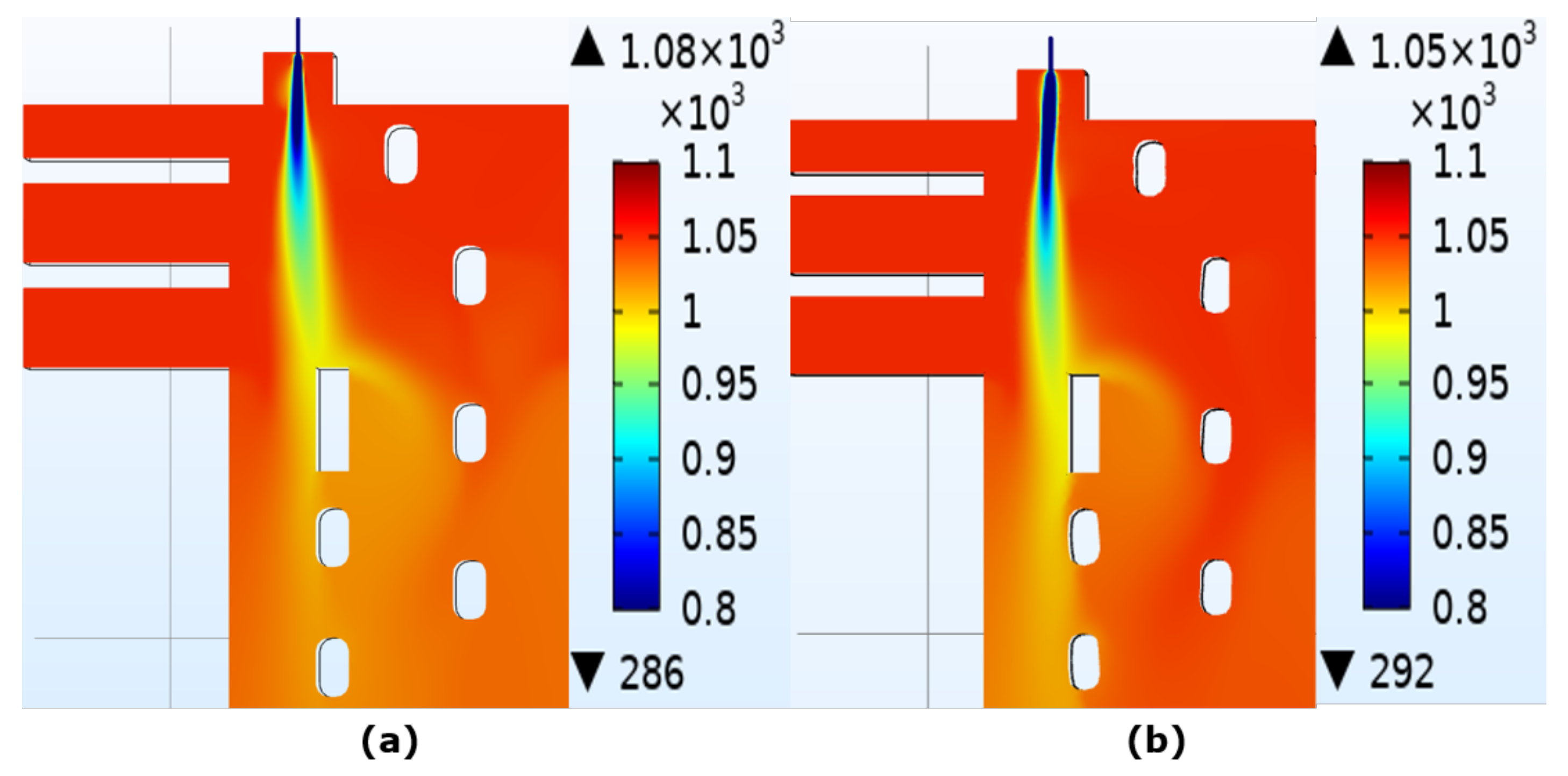
The non-isothermal results of the baseline model with Mesh 1 are presented in Figure 8. The y+ values for the model range from 11.1 to 287. However, the y+ values are close to 11.06 in most of the region. The baseline model is decided on the basis of the qualitative behaviour of the solution. The solution of this model for velocity, turbulent viscosity ratio, and temperature are as shown in Figure 8a–c respectively, aligns with the expected physical behaviour. The baseline model serves as the reference for the analysis of the other meshes studied in this paper.

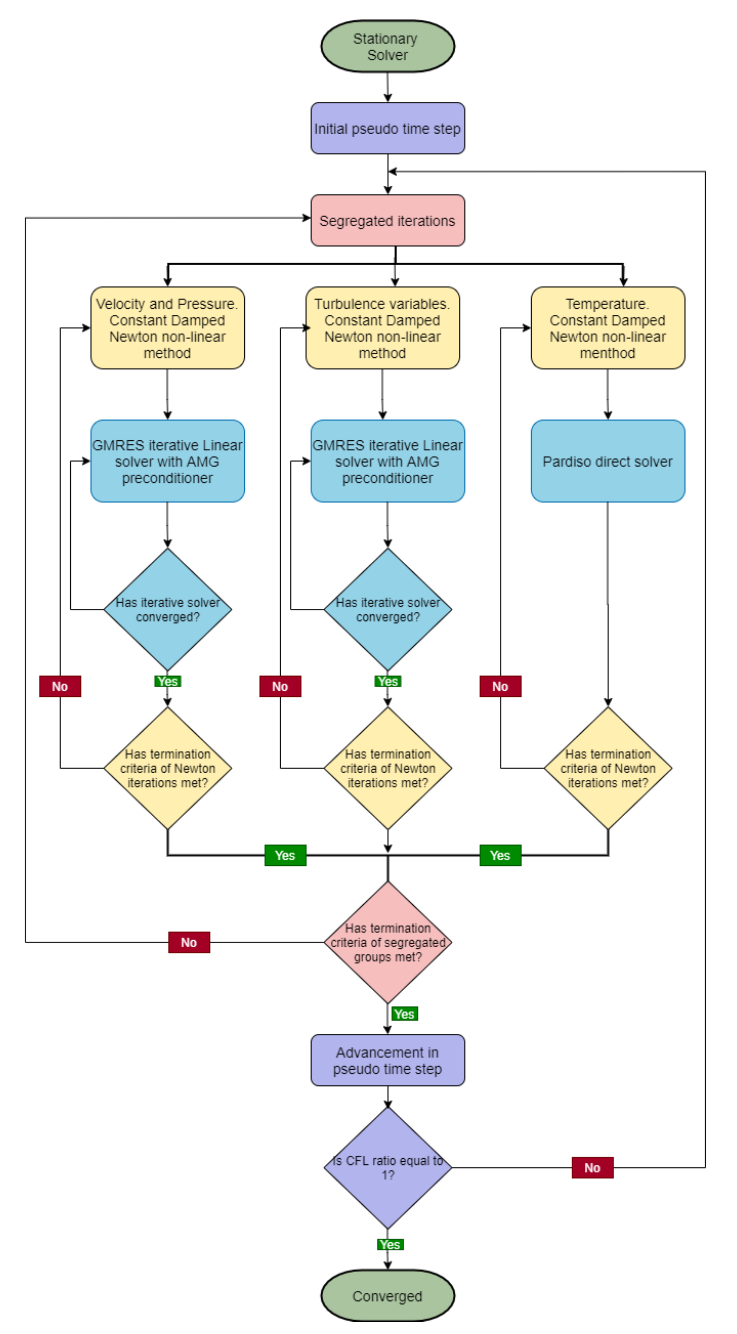
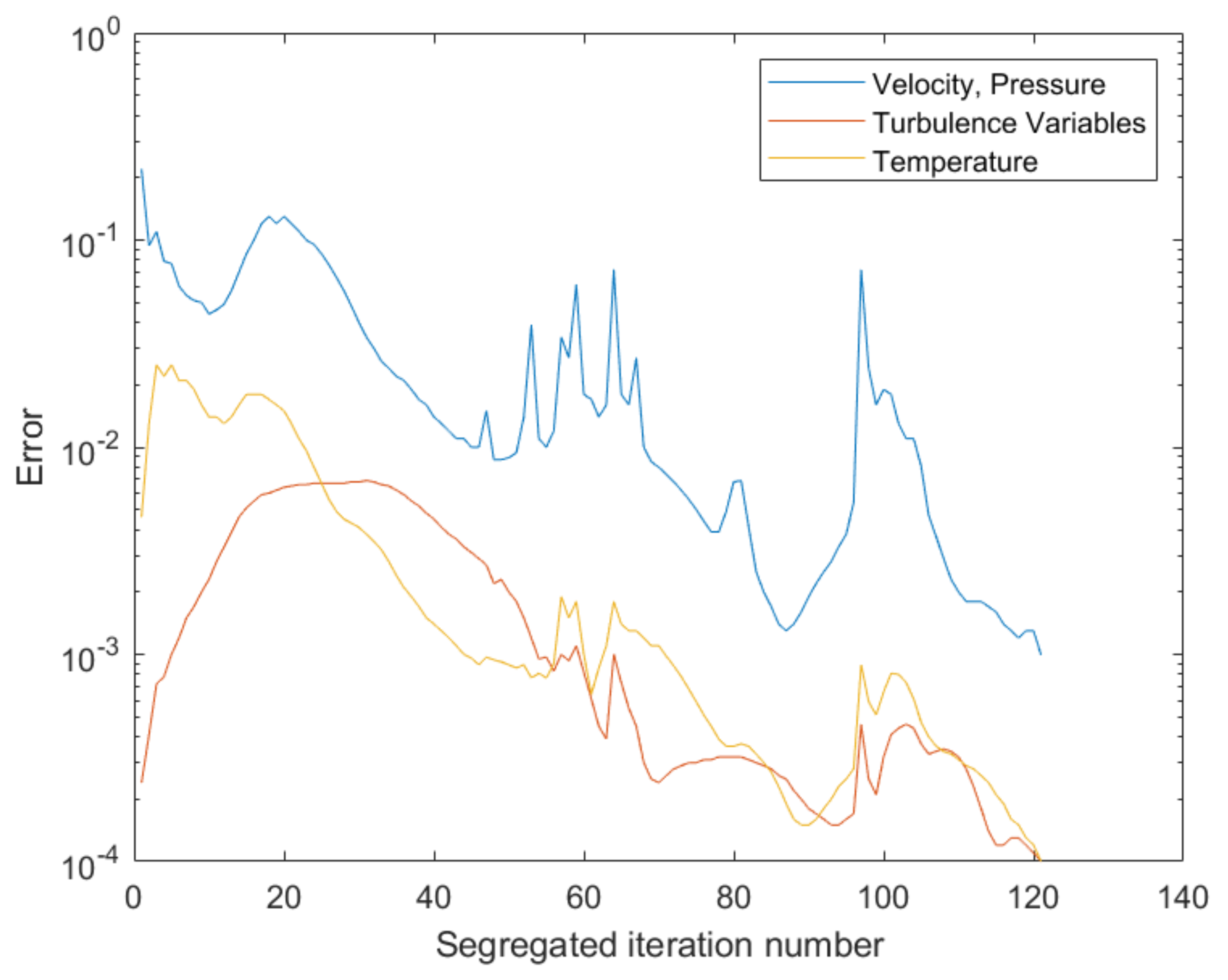
As discussed in Figure 7, the non-isothermal model is solved by segregating physics into different groups. The convergence behaviour of the three segregated groups is as shown in Figure 9. The stopping criteria for the solver is set at relative tolerance of ${10}^{-3}$ which is sufficient for the current application. The solver is converged if relative tolerance exceeds the relative error.

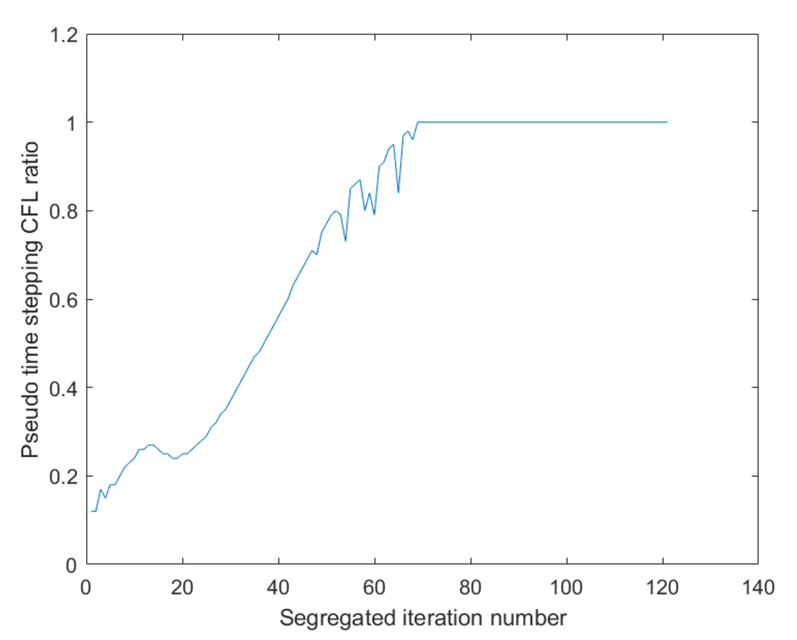
The progress of CFL number is quantified based on the pseudo time stepping CFL ratio which is defined as $min(log(CFL)/log(CF{L}_{\infty }),1)$ where, $CF{L}_{\infty }={10}^4$. The progress of the simulation is completed when the pseudo time stepping CFL ratio is 1. Figure 10 shows the progress of the pseudo time stepping CFL ratio with respect to the segregated iteration number. As can be seen in the figure, the pseudo time stepping CFL ratio steadily increases to 1 providing better stabilization.

3.2. Non-Isothermal Effect on Baseline Model with Mesh 1

The non-isothermal effect on the velocity and the turbulent viscosity ratio is shown in Figure 11. Due to the varying density, the jet is penetrating further into the furnace. The temperature coupling steadily increases the temperature of the jet reducing the density. This results in the deeper penetration of the jet. The effect of obstacles by the tie brick is more significant and changes the flow dynamics in the furnace for the coupled equations. Therefore, while studying aerodynamics in the anode baking furnace, it is important to consider the non-isothermal flow model.

3.3. Comparison of Mesh 1 and Mesh 2

In the previous paper [10], the results with the meshing carried out by COMSOL are discussed. Due to the physically unrealistic computation of turbulent viscosity ratio with the COMSOL mesh, an alternate meshing tool, cfMesh, is considered for the study. After confirming the precise turbulent viscosity ratio with this meshing tool, mesh with comparable element sizes is prepared with the default mesher from COMSOL. 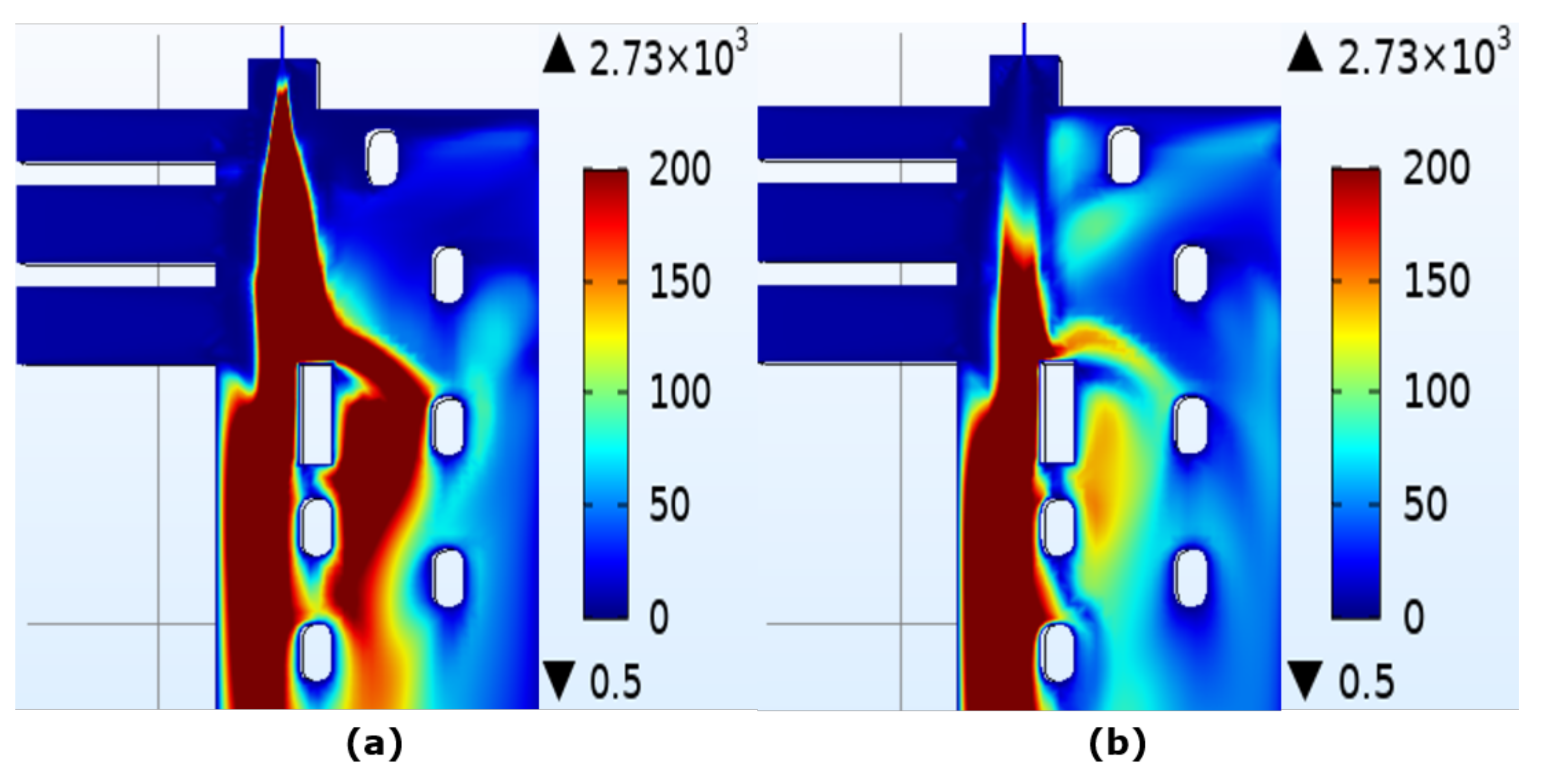The details of these meshes are discussed in Section 2.3. 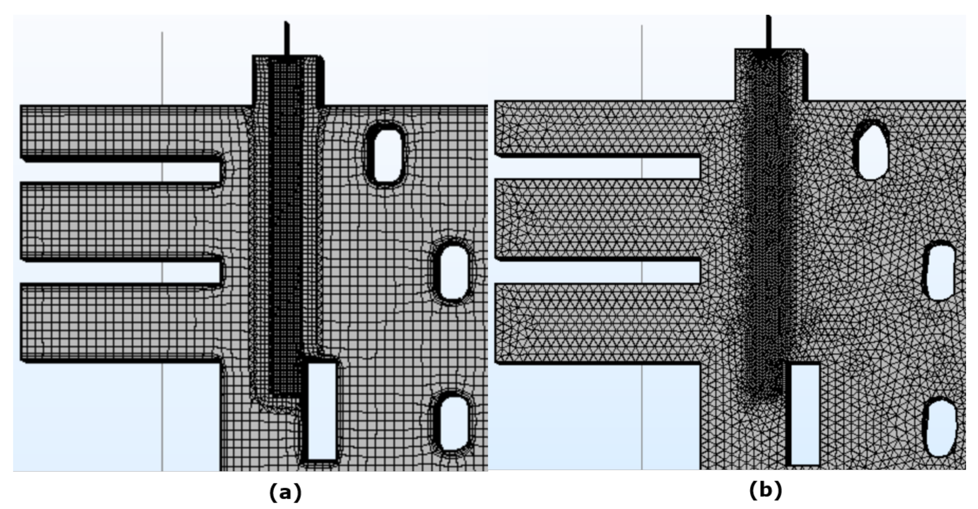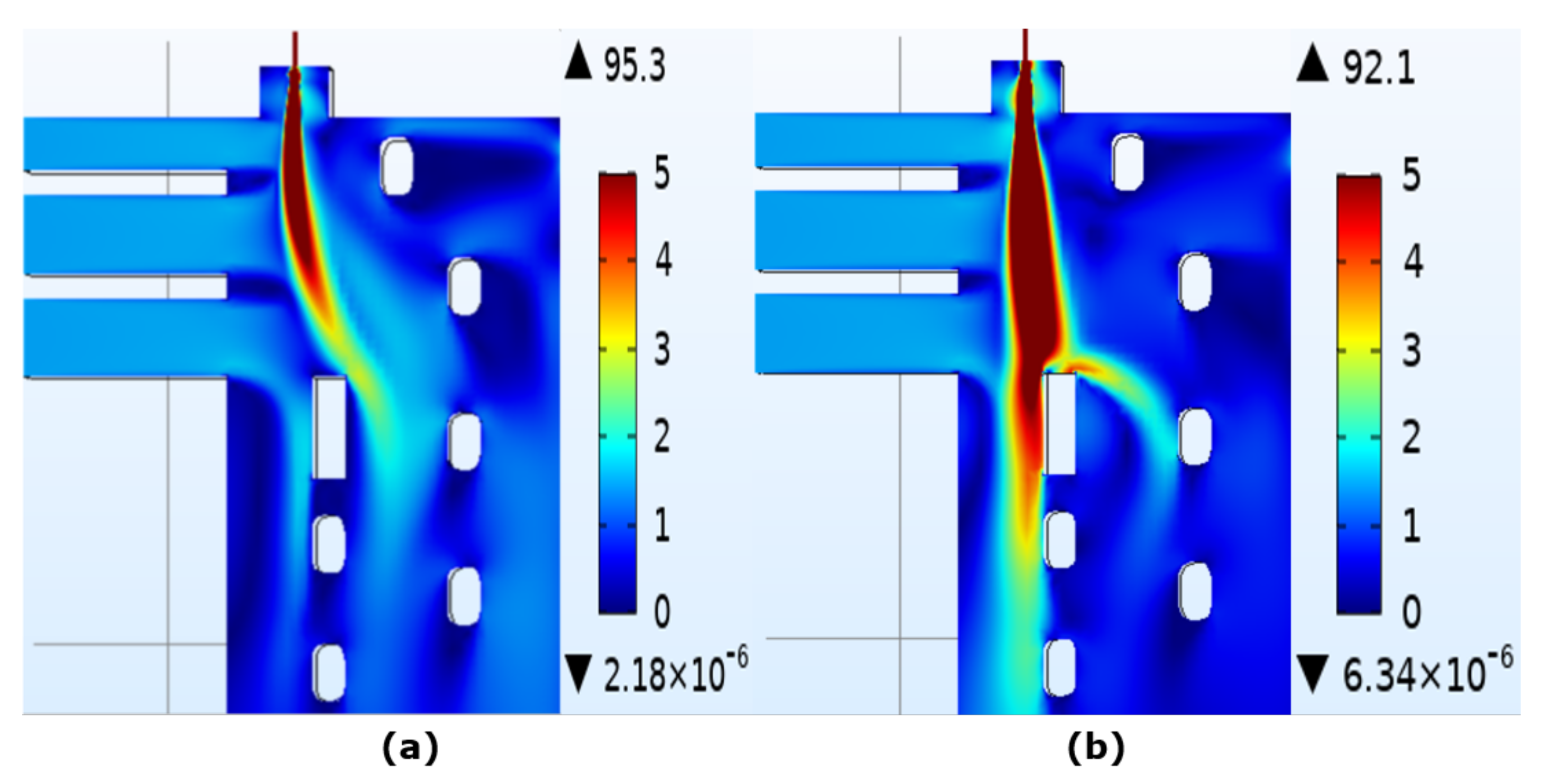The comparison of velocity with the two meshing techniques, namely, by COMSOL (Mesh 2) and cfMesh (Mesh 1) is provided in Figure 12a,b, respectively. It can be observed that the velocity magnitude from Mesh 1 develops symmetrically as opposed to Mesh 2 in which it is bent towards left. Due to the symmetrical development of jet in Mesh 1, the jet encounter the first tie-brick and have a stream split towards the right. As opposed to this, the jet with Mesh 2 does not encounter the brick to a significant extent. Therefore, most of the flow happens at the left of the first tie-brick for Mesh 2. It should be noted that the number of elements required to obtain results with COMSOL is approximately 8 times higher as compared to the cfMesh mesh.

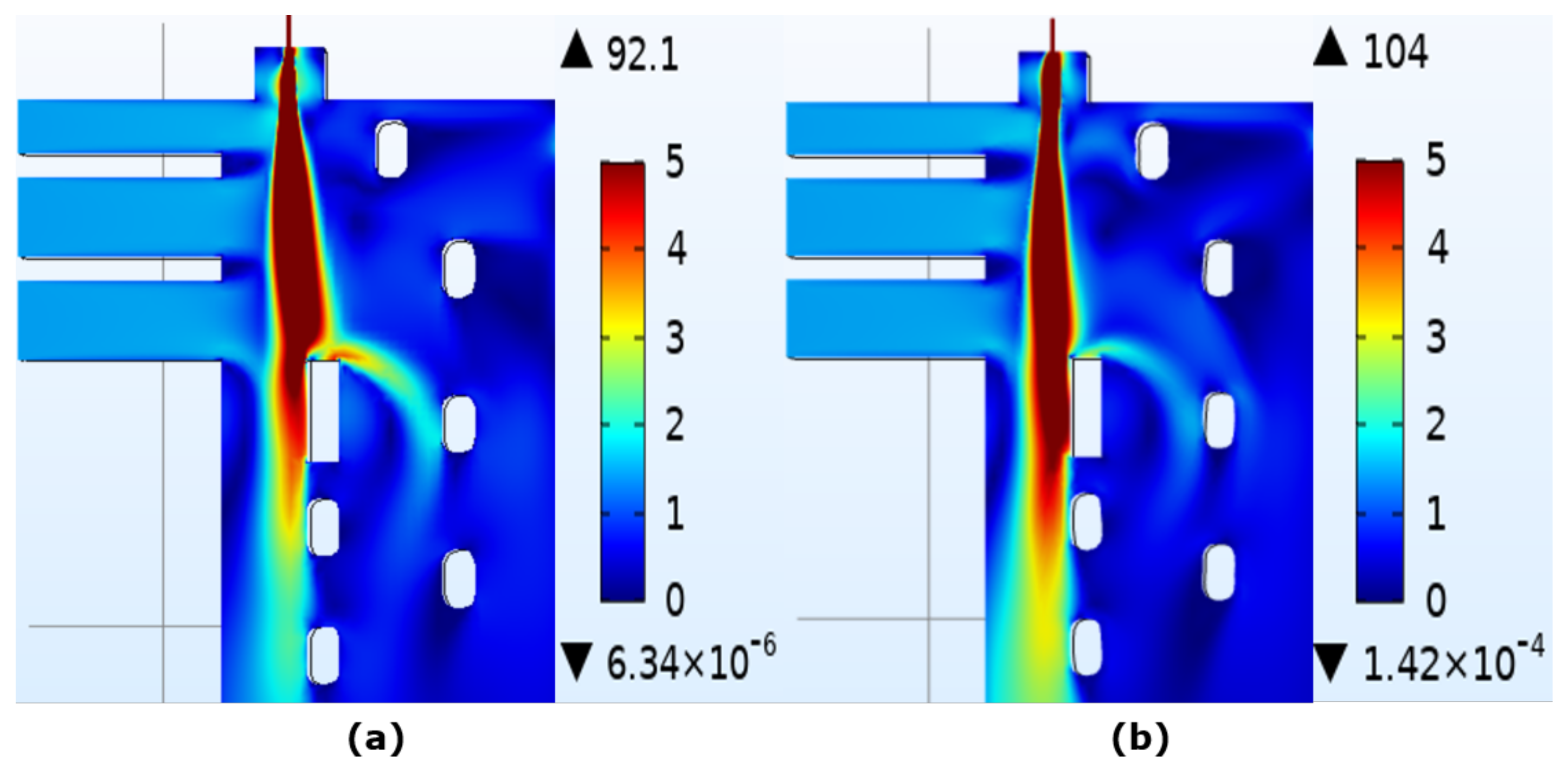
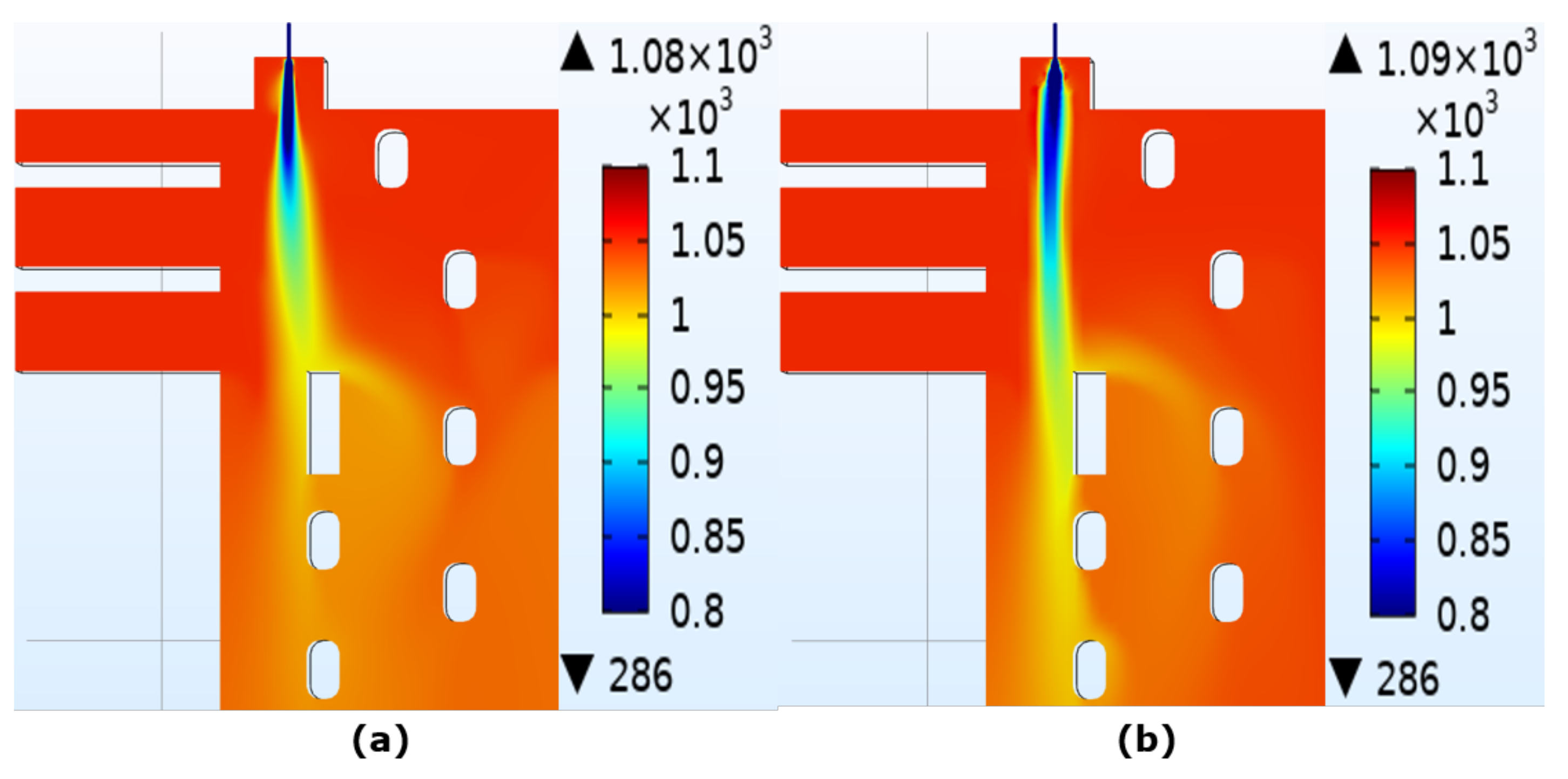
The temperature comparison (Figure 13) for the two meshes, Mesh 1 and Mesh 2 is similar to the velocity comparison. It follows the pattern of flow dynamics. The difference between the temperature distribution obtained by the two meshes is again due to the way the jet encounters the first tie-brick. This shows the strong coupling of temperature and flow dynamics based on the density.

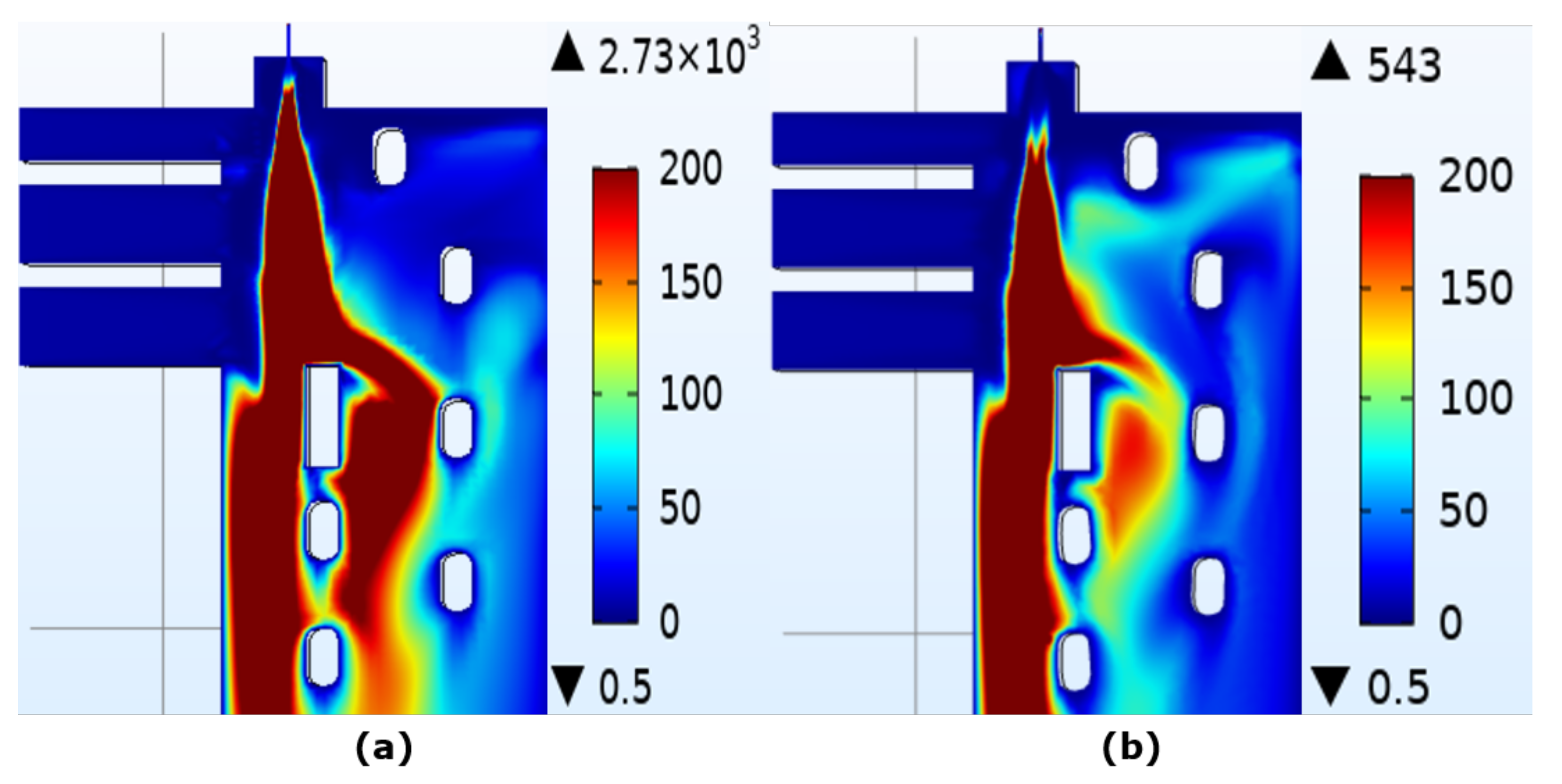
Further comparison of turbulent viscosity ratio with the two meshing techniques is as shown in Figure 14a,b, respectively. It is important to analyze the turbulent quantities since the combustion modeling that follows from the turbulent flow modeling depends on the turbulence parameters. It can be observed that the turbulent viscosity ratio immediately near the fuel outlet is lower with the COMSOL mesh as compared to the cfMesh. Moreover, the turbulent viscosity ratio starts dissipating with the COMSOL mesh. Both these observations can be attributed to the higher numerical diffusion with the COMSOL mesh. Due to the dissipation with the COMSOL mesh, the flow dynamics downstream such as near the obstacle of the tie-brick are affected. Since the NOx formation is restricted to this region, the changes in the flow dynamics are translated into the thermal NOx formation phenomena as well.

3.4. Comparison of Mesh 1 and Mesh 3

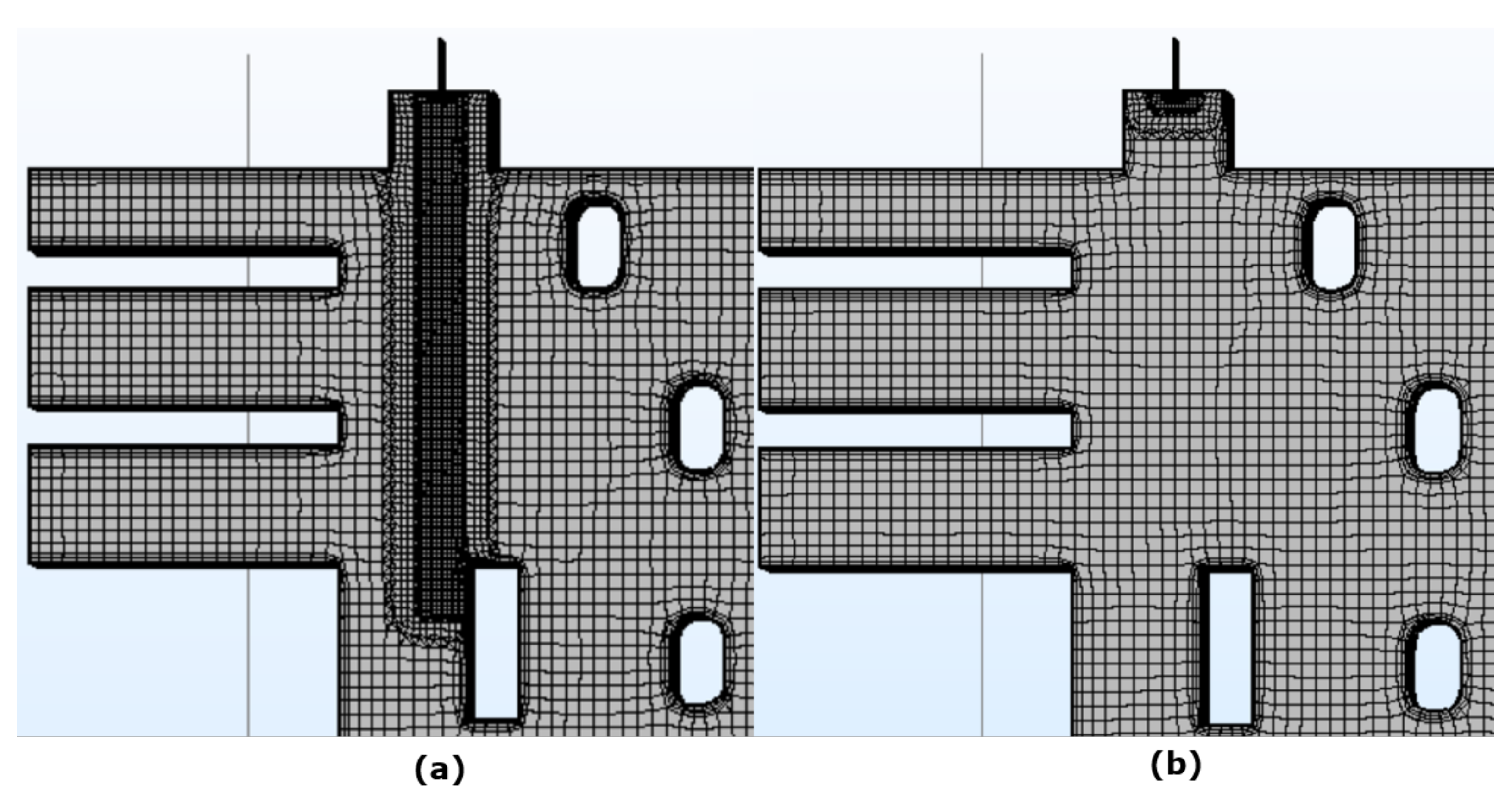
The idea of local mesh refinement in the region of interest is well known. For large models such as the industrial furnaces, it is important to identify the region which is sensitive to the flow dynamics. In the present study, such a region lies beneath the fuel outlet. Therefore, in this section, the sensitivity of the results on the local refinement in the region of jet development is studied. Two meshes with varying local refinement (Mesh 1 and Mesh 3) are generated by cfMesh software. The representation and description of these meshes are given in the mesh section (Figure 6). 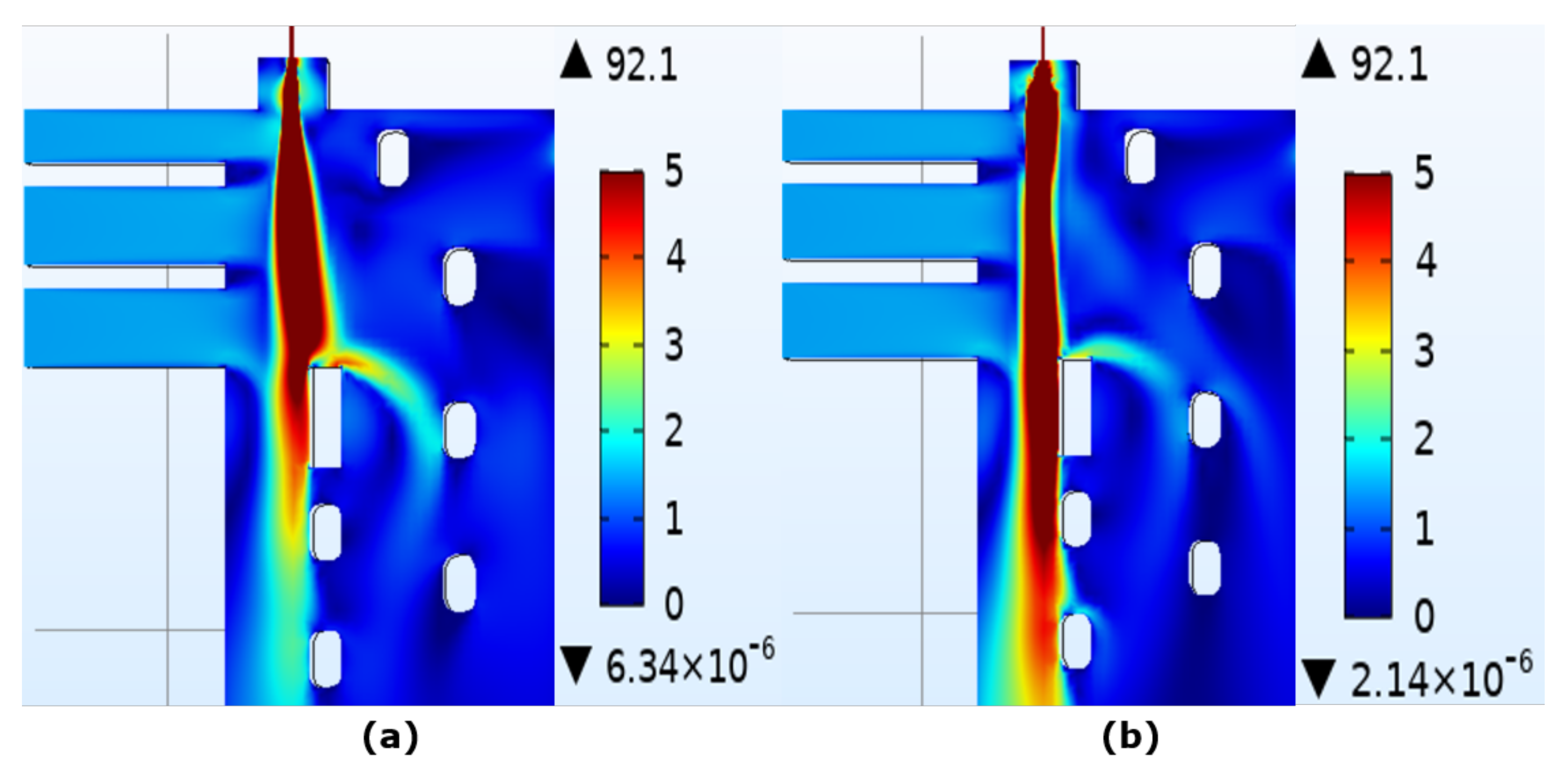The comparison of velocity magnitude with the two meshes is as shown in Figure 15). The quick analysis suggests that the results of Mesh 3 is less diffused as compared to that of Mesh 1 which is refined underneath the fuel outlet. However, the contradiction in the results can be better explained with the help of comparison of turbulent viscosity ratio presented in Figure 16. The effect of local refinement is prominent on the turbulent viscosity ratio as compared to the velocity magnitude. The mesh that does not have local refinement (Mesh 3) has a lower turbulent viscosity ratio immediately near the fuel outlet as compared to the one with local refinement. The effect of turbulence is better captured with locally refined mesh. The effect of better refinement underneath the jet (Mesh 1) resolves velocity magnitude in such a way that it encounters the first obstacle without bending the jet. In case of the jet that does not have refinement, the jet is bent towards left and does not encounter the obstacle. Therefore, the kinetic energy for the jet with Mesh 3 is not dissipated resulting into longer jet. Therefore, the numerical diffusion effect can not be concluded from the velocity magnitude plot. The deeper penetration of the jet with Mesh 3 is due to the bending of the jet towards left. The comparison of turbulent viscosity ratio provides better judgement of the diffusive behaviour of Mesh 3 as compared to Mesh 1. The comparison of temperature with the two meshes shown in Figure 17) follows the velocity magnitude plot. Studying such effects near the burner is important since this is the region where NOx is generated.

3.5. Realizable k-$ϵ$ Model

The realizable k-$ϵ$ model is the improved model of the standard k-$ϵ$ model in which the dependence of mean flow distortion on turbulent dissipation is accounted for. The realizable k-$ϵ$ model is known to provide well-quantified results for the round jets. The numerical diffusion introduced by the realizable k-$ϵ$ model is lesser than compared to the standard k-$ϵ$ model. However, the convergence with the realizable k-$ϵ$ model is not easy to achieve for complex geometries such as anode baking furnace. The baseline model Mesh 1 explained in the previous section fails to converge for the realizable k-$ϵ$ model. In the case of the realizable k-$ϵ$ model, more constraints are introduced. There are several studies carried out to analyze these constraints which would provide techniques to achieve convergence with the realizable k-$ϵ$ model.

The discussion on the results of the standard k-$ϵ$ model suggests that the higher numerical diffusion introduced by the low-quality mesh affects the results, especially the turbulent viscosity ratio. The turbulent viscosity is of primary importance with respect to the difference of standard and realizable k-$ϵ$ model. Therefore, the non-convergence of the realizable k-$ϵ$ model might be due to the insufficient mesh resolution at the fuel outlet. A test case is run on the 2D model to recognize the effect of mesh resolution in the direction perpendicular to the jet flow. The mesh with higher resolution shows convergence whereas the model fails to converge for the mesh with lower resolution. However, the baseline model modified by removing the fuel inlet also fails to converge. This suggests that apart from the sufficient resolution of mesh at the fuel outlet, other regions needs to be investigated further to achieve convergence.

Moreover, other factors that might be responsible for the non-convergence of the realizable k-$ϵ$ model are studied including the stabilization techniques. COMSOL Multiphysics applies consistent and inconsistent stabilization techniques as described in the simulation details section. The inconsistent stabilization technique introduces isotropic artificial diffusion to the equation. If the flow is convection dominated that is, for the higher Peclet number, the numerical problem may become unstable. Isotropic diffusion in such respect may be used as a stabilization technique. The extent of the isotropic diffusion can be controlled by the stabilization parameter which ranges from 0 to 1. The stabilization parameter, that controls the extent of the artificial diffusion is varied and the effect on the convergence behavior is analyzed. The addition of artificial diffusion with higher stabilization parameter aids in convergence compensating the accuracy. As discussed in the earlier sections, the higher numerical diffusion (added artificially in this case) impacts the turbulent viscosity ratio more than velocity and temperature.

The role of the solver in the non-convergence is discussed. The non-linear flow solver of COMSOL Multiphysics is described in Figure 7. The convergence of the segregated solver is achieved when each non-linear segregated step is converged. Furthermore, for each non-linear segregated step, a damped Newton method is applied in which the solver assumes several linear steps. To understand the effect of the tolerance of the linear solver on the convergence, a test case with a simple rectangular channel is considered. The iso-thermal non-linear solver is run for various tolerances of the linear solver. However, even with the more stringent tolerance criteria such as ${10}^{-14}$ of GMRES iterative linear solver, the convergence behavior is similar to more relaxed tolerance criteria of ${10}^{-3}$. This suggests that the non-convergence of the realizable k-$ϵ$ model is not dependent on the accuracy of the linear solver.

As described in the simulation details, the pseudo time stepping accelerates the convergence towards a steady-state by introducing a pseudo time step. The pseudo time step is related to the local CFL number and can be made more stringent with the PID regulator. Another test case on a simpler geometry is carried out. It is observed that as compared to the default time step, the convergence with the smaller time steps is decreasing faster. However, the progress of the CFL ratio now becomes extremely slow. This suggests that it generates better initial guesses for the Newton iteration in the next time steps. These improved initial guesses however fail to compensate for the mesh resolution.

The study of the realizable k-$ϵ$ model with detailed analysis is still in progress. It is important to obtain results of velocity, temperature, and turbulent viscosity ratio to a sufficient resolution in order to compute accurate NOx prediction.

4. Conclusions

A detailed analysis of turbulent flow modeling has been carried out and it can be concluded that the turbulent quantities are more sensitive to the mesh as compared to the velocity. The non-Cartesian mesh obtained by the COMSOL default solver introduces high diffusion leading to physically incorrect computation of turbulent viscosity ratio. To obtain the Cartesian mesh, the cfMesh software is used. The workflow for generating meshes with cfMesh software and importing it into COMSOL has been developed. The two meshing techniques (the default COMSOL mesher and cfMesh meshing tool) are compared and it can be concluded that the Cartesian mesh generated by cfMesh is required for accurate computation of turbulent viscosity ratio. Furthermore, the local refinement in the region of interest, underneath the burner outlet, in this case, improves the computation of turbulent viscosity ratio. Such refinement should be employed for accurate prediction of NOx which is highly dependent on the aerodynamics. The standard k-$ϵ$ model is robust towards the convergence of the anode baking model even for the Cartesian refined mesh which has less numerical diffusion. The realizable k-$ϵ$ model that accounts for a more accurate definition of turbulent viscosity needs further investigation to obtain accurate results.

References

1. Gaba, A.; Felicia, S. Reduction of Air Pollution by Combustion Processes. In The Impact of Air Pollution on Health, Economy, Environment and Agricultural Sources; IntechOpen: London, UK, 2011. [Google Scholar] [CrossRef] [Green Version]
2. Richard, C.F.; Seinfeld, J.H. Fundamentals of Air Pollution Engineering; Prentice Hall: Englewood Cliffs, NJ, USA, 1988; ISBN 0-13-332537-7. Available online: http://authors.library.caltech.edu/25069/ (accessed on 15 September 2020).
3. Baukal, C.E. Industrial Combustion Pollution and Control. In Environmental Science & Pollution; CRC Press: Boca Raton, FL, USA, 2003; ISBN 9780367578459. [Google Scholar]
4. Bui, R.T.; Charette, A.; Bourgeois, T. Simulating the process of carbon anode baking used in the aluminum industry. Metall. Trans. B 1984, 15, 487–492. [Google Scholar] [CrossRef]
5. Grégoire, F.; Gosselin, L. Comparison of three combustion models for simulating anode baking furnaces. Int. J. Therm. Sci. 2018, 129, 532–544. [Google Scholar] [CrossRef]
6. Tajik, A.R.; Shamim, T.; Ghoniem, A.F.; Abu Al-Rub, R.K. The effects of flue-wall design modifications on combustion and flow characteristics of an aluminum anode baking furnace-CFD modeling. Appl. Energy 2018, 230, 207–219. [Google Scholar] [CrossRef]
7. Tajik, A.R.; Shamim, T.; Ghoniem, A.F.; Abu Al-Rub, R.K. CFD Modelling of NOx and Soot Formation in Aluminum Anode Baking Furnace. In ASME International Mechanical Engineering Congress and Exposition; American Society of Mechanical Engineers: Two Park Avenue, NY, USA, 2018; Volume 52118. [Google Scholar]
8. Besson, S.; Bache, S.; Bourgier, A.; Schneider, J.P.; Conte, T. Modelling of Gas Injection on Anode Baking Furnace and Application to Operations. In Light Metals; Springer: Cham, Switzerland, 2020; pp. 1196–1202. [Google Scholar]
9. Donea, J.; Huerta, A. Finite Element Methods for Flow Problems; John Wiley & Sons: Hoboken, NJ, USA, 1986. [Google Scholar]
10. Nakate, P.; Lahaye, D.; Vuik, C.; Talice, M. Computational study of the anode baking industrial furnace. In Industrial Combustion Symposium; The American Flame Research Committee (AFRC): Lakewood Ranch, FL, USA, 2019. [Google Scholar]
11. Juretic, F. cfMesh Version 1.1 Users Guide. Available online: http://cfMesh.com/wp-content/uploads/2015/09/User_Guide-cfMesh_v1.1.pdf (accessed on 15 September 2020).
12. Grotjans, H.; Menter, F. Wall Functions for General Application CFD Codes. ECCOMAS 98. In Proceedings of the 4th Computational Fluid Dynamics Conference, Athens, Greece, 7–11 September 1998; John Wiley & Sons: Hoboken, NJ, USA, 1998; pp. 1112–1117. [Google Scholar]
13. COMSOL Multiphysics Version 5.4 Reference Manual. Available online: https://doc.comsol.com/5.4/doc/com.comsol.help.comsol/COMSOL_ReferenceManual.pdf (accessed on 15 September 2020).
14. Hughes, T.J.; Franca, L.P.; Balestra, M. A new finite element formulation for computational fluid dynamics: V. Circumventing the Babuška-Brezzi condition: A stable Petrov-Galerkin formulation of the Stokes problem accommodating equal-order interpolations. Comput. Methods Appl. Mech. Eng. 1986, 59, 85–99. [Google Scholar] [CrossRef]
15. COMSOL Multiphysics Version 5.4 CFD Users Guide. Available online: https://doc.comsol.com/5.4/doc/com.comsol.help.cfd/CFDModuleUsersGuide.pdf (accessed on 15 September 2020).
Figure 1. The schematic representation of the anode baking furnace. The left-most picture is the photograph from the actual furnace showing the exit of the flue channel. The right-most picture shows a photograph of the burner through which fuel is injected.
Fluids 06 00046 g001
Figure 2. The schematic representation of different zones in the anode baking furnace based on the transfer of heat. The sections presented in the red box are in the heating zone. One section (section 7) is studied in this paper due to its importance with respect to the NOx generation.
Fluids 06 00046 g002
Figure 3. The 3D geometry of the heating section of the anode baking furnace model.
Fluids 06 00046 g003
Figure 4. The Cartesian mesh generated by the software cfMesh (Mesh 1) of the heating section of the anode baking furnace.
Fluids 06 00046 g004
Figure 5. Mesh at the symmetry plane (Z = 0.27 m) in the flue wall prepared in (a) cfMesh (Mesh 1) and (b) COMSOL (Mesh 2) software respectively.
Fluids 06 00046 g005
Figure 6. Mesh at the symmetry plane (Z = 0.27 m) in the heating section prepared in cfMesh (a) with jet refinement (Mesh 1) and (b) without jet refinement (Mesh 3).
Fluids 06 00046 g006
Figure 7. The flowchart of non-isothermal non-linear flow solver in COMSOL Multiphysics.
Fluids 06 00046 g007
Figure 8. The color plots of (a) velocity (b) turbulent viscosity ratio and (c) temperature at the symmetry plane (Z = 0.27 m) of baseline model with Mesh 1.
Fluids 06 00046 g008
Figure 9. The convergence plot for the three segregated groups of different physics for baseline model with Mesh 1. The convergence is plotted for the step 4 from Table 8.
Fluids 06 00046 g009
Figure 10. The Pseudo time stepping CFL ratio for the baseline model with Mesh 1.
Fluids 06 00046 g010
Figure 11. The color plots of velocity magnitude at the symmetry plane (Z = 0.27 m) for (a) uncoupled and (b) coupled flow and energy equations for baseline model with Mesh 1.
Fluids 06 00046 g011
Figure 12. The color plots of velocity magnitude at the symmetry plane (Z = 0.27 m) generated by (a) cfMesh (Mesh 1) and (b) COMSOL mesh (Mesh 2).
Fluids 06 00046 g012
Figure 13. The color plots of temperature at the symmetry plane (Z = 0.27 m) generated by (a) cfMesh (Mesh 1) and (b) COMSOL mesh (Mesh 2).
Fluids 06 00046 g013
Figure 14. The color plots of turbulent viscosity ratio at the symmetry plane (Z = 0.27 m) generated by (a) cfMesh (Mesh 1) and (b) COMSOL mesh (Mesh 2).
Fluids 06 00046 g014
Figure 15. The color plots of velocity magnitude at the symmetry plane (Z = 0.27 m) generated by cfMesh software (a) with jet refinement (Mesh 1) and (b) without jet refinement (Mesh 3).
Fluids 06 00046 g015
Figure 16. The color plots of turbulent viscosity ratio at the symmetry plane (Z = 0.27 m) generated with the mesh of cfMesh software (a) with jet refinement (Mesh 1) and (b) without jet refinement (Mesh 3).
Fluids 06 00046 g016
Figure 17. The color plots of temperature at the symmetry plane (Z = 0.27 m) generated by cfMesh software (a) with jet refinement (Mesh 1) and (b) without jet refinement (Mesh 3).
Fluids 06 00046 g017