
Numerical Simulation of Dynamic Fluid-Structure Interaction with Elastic Structure–Rigid Obstacle Contact


1
Laboratoires Analyse, Optimisation et Traitement de l’Information, Faculté des Sciences Exactes et Informatique, Université Mohammed Seddik BenYahia, BP 98 Ouled Aissa, Jijel 18000, Algeria
2
Département de Mathématiques, Institut de Recherche en Informatique, Mathématiques, Automatique et Signal, Université de Haute Alsace, 6, Rue des Frères Lumière, 68093 Mulhouse, France
*
Author to whom correspondence should be addressed.
Fluids 2021, 6(2), 51; https://0-doi-org.brum.beds.ac.uk/10.3390/fluids6020051
Submission received: 8 November 2020
/
Revised: 15 January 2021
/
Accepted: 20 January 2021
/
Published: 22 January 2021
(This article belongs to the Special Issue Fluid Structure Interaction: Methods and Applications)
Abstract
:An implicit scheme by partitioned procedures is proposed to solve a dynamic fluid–structure interaction problem in the case when the structure displacements are limited by a rigid obstacle. For the fluid equations (Sokes or Navier–Stokes), the fictitious domain method with penalization was used. The equality of the fluid and structure velocities at the interface was obtained using the penalization technique. The surface forces at the fluid–structure interface were computed using the fluid solution in the structure domain. A quadratic optimization problem with linear inequalities constraints was solved to obtain the structure displacements. Numerical results are presented.
1. Introduction
The Arbitrary Lagrangian Eulerian (ALE) method was successfully employed for solving fluid–structure interaction problems, see [1]. The fluid equations were written in the moving mesh which matches the structure displacement. This method was not adapted for a structure–rigid obstacle contact when the topology of the fluid domain changed from double to simply connected. Some authors have introduced a gap between the elastic structure and the rigid obstacle as in [2].
Some methods exist for solving fluid–structure interaction problems using a fixed mesh for the fluid domain. We recall some of them. The immersed boundary method, see the survey paper [3], was designed originally for a thin structure. It was extended to a thick, viscous hyper-elastic structure in [4], where it was assumed that the fluid and structure densities and viscosities were the same. The fictitious domain with distributed Lagrange multiplier [5] was employed for the simulation of flow around moving rigid bodies. The extension to a visco-elastic structure was proposed in [6]. The densities, respectively, the viscosities of fluid and visco-elastic materials were not the same. For a rigid thick body immersed in an incompressible fluid, the convergence of a penalization method was presented in [7] and the extended finite element method (XFEM) was used in [8]. Nitsche-XFEM was used in [9] for a thin elastic structure immersed in an incompressible fluid.
Concerning the fluid–structure interaction with a structure–rigid obstacle contact, we can cite some works. In [10], for a 1D elastic structure, the Lagrange multiplier was employed to compute the interface forces. The Uzawa algorithm was used to handle the contact. An extension to a 3D nonlinear shell was presented in [11]. An approach using the extended finite element method (XFEM) and a mortar contact formulation was proposed in [12]. In [13], an immersogeometric variational framework for fluid–structure interactions with application to a 3D heart valve was presented. In recent papers, a monolithic Eulerian framework with remeshig was used in [14], a stabilised immersed methodology on hierarchical b-spline grids was employed in [15], the cut finite element method was used in [16], a Nitsche-based formulation with artificial fluid in the gap between structure and obstacle was presented in [17].
In [18], the fictitious domain method with penalization presented in [19,20] was used in order to handle the contact between a linear elastic structure and a rigid obstacle in a fluid–structure interaction problem. The surface forces at the fluid–structure interface were computed using the fluid solution in the structure domain. The equality of the fluid and structure velocities at the interface was obtained using the penalization technique. In the present paper, we present a dynamic fluid–structure interaction problem when the elastic structure is in contact with a rigid obstacle. The fluid was modeled by the Stokes as well as by the Navier–Stokes equations.
2. Fluid–Structure Interaction with Contact: The Mathematical System
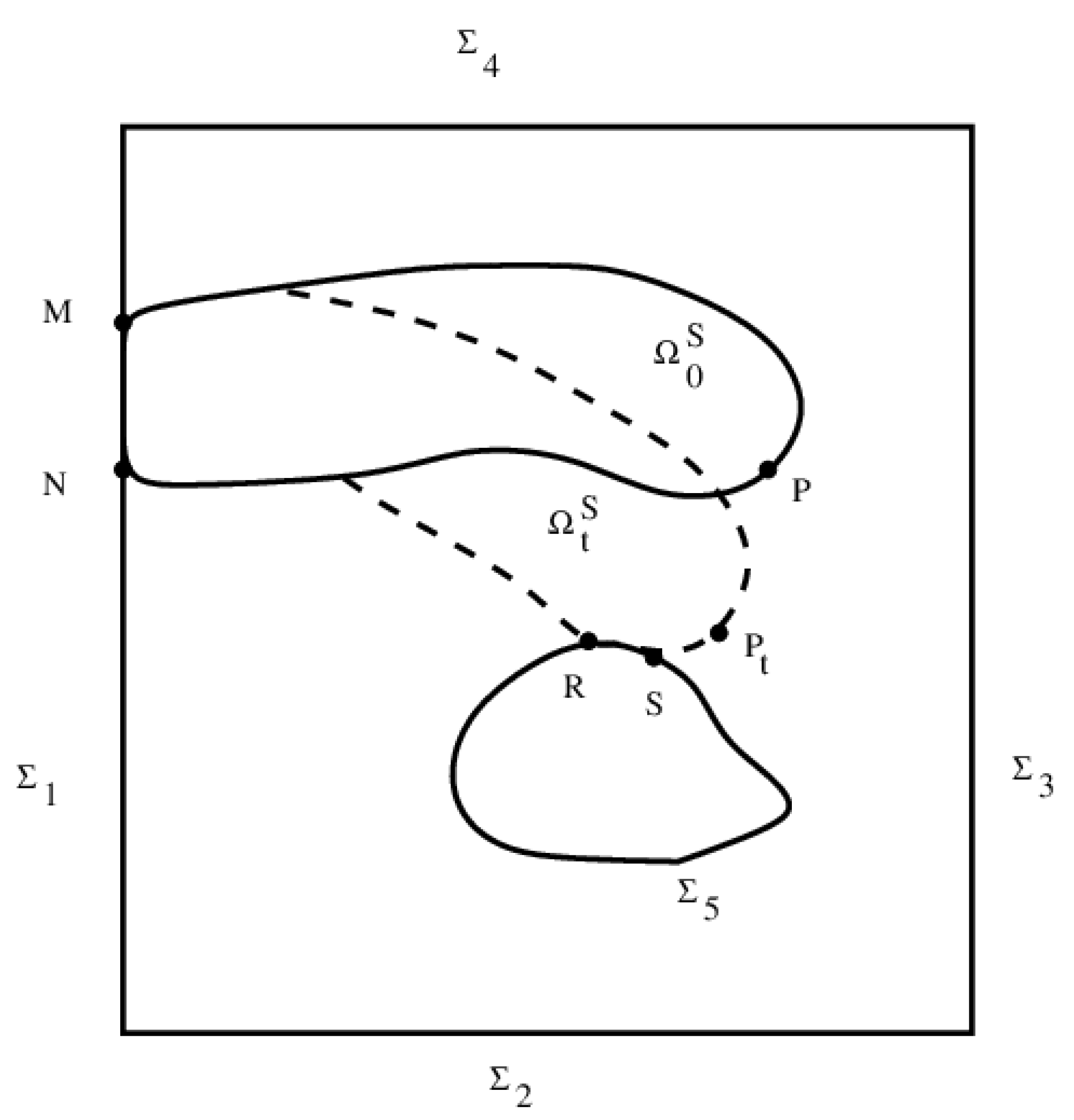
The undeformed structure domain has Lipschitz boundary . On the displacement is zero, on surface loads are imposed and a subset of will touch a rigid obstacle, after deformation. In Figure 1, we have , , .
The structure displacement will be denoted by . A point in the undeformed structure domain will occupy the position in the deformed structure domain . We set and .
The bounded domain of boundary is the rigid obstacle. In the case of an elastic structure–rigid obstacle contact, we have . To simplify, we assume that is a connected Lipschitz curve. We have , where , see Figure 1. The conclusions are the same if we replace by a finite union of Lipschitz arches.
The fluid domain has the boundary and . In Figure 1, D is a rectangle with a hole of boundary . The top side is the inflow, the bottom side is the outflow, the left side and the right side represent the wall.
We suppose that and the fluid occupies . The set is not necessary a Lipschitz domain when the structure touches the rigid obstacle.
The system to be solved is to find the structure displacement , the fluid velocity and the fluid pressure such that:
where are the applied volume forces and is the unit outward vector normal to . Additionally, we define and the unit outward vector normal to . The Equations (13)–(15) represent the initial conditions, , , are given.
In (5), is the imposed velocity. If no-slip boundary conditions are prescribed at , since the fluid is incompressible, then the volume of the structure is constant, too. In our case, it is not necessary to add the same restriction on the volume of the structure, even when because we use (7) at the outflow boundary .
For (12), we followed [21] (Theorem 5.3-1, p. 210), is the unit vector normal to at the point , oriented to the exterior of D. We point out that the value of is not given. The meaning of (12) is that the force acting on the structure on the contact zone is parallel to and it has opposite direction. In the case of linear elasticity, (12) could be approached by
where is the unit tangential vector to .
If the elastic structure is not in contact with the obstacle , the Equations (9)–(12) are replaced by
We have denoted by and the Cauchy stress tensors of the structure and fluid, respectively. The structure equations are written using Lagrangian coordinates , are the Lamé coefficients, and is the unit matrix. The Eulerian coordinates have been used for fluid equations , is the viscosity and . The mass densities are denoted by and .
To the best of our knowledge, there are no reported results for fluid–structure interaction with a contact. However, without a structure–obstacle contact, there are reported results for fluid–structure interactions. In general, in the literature, the domain of the fluid is assumed to be Lipschitz. However, when the structure touches the rigid obstacle, the fluid domain is not necessary a Lipschitz domain. Existing results for fluid–structure interactions are presented in [19,20,22,23] and the references are given there. In [19,20,22], the fictitious domain method was used and this technique could be more appropriate to handle the structure–obstacle contact in the fluid–structure interaction framework.
3. Approximation of the Elastodynamics Frictionless Contact Problem
We analyze, in this section, the linear dynamic elasticity equations with a frictionless contact. In , volume forces are imposed and on surface loads are prescribed. The structure is fixed along . We recall that .
Let be a function describing a part of the top boundary of the obstacle. We set its graph by
and its epigraph by
The non-penetration condition of the elastic structure into the obstacle gives
A point belongs to the coincidence set at time instant t if . In the case of linear elasticity, see [24], the condition (16) can be replaced by
Denoting by the first-order Sobolev space, let us introduce the Hilbert space
the bi-linear form ,
and the closed, convex and non-empty set
We assume , , , . We can write the linear elastodynamics frictionless contact problem as a variational inequality: find such that
The existence for dynamic linear elasticity with frictionless contact in an arbitrary domain is still open, see the monograph ([25] Section 4.1). Existence and uniqueness results for an elastodynamics contact problem were obtained: in [26] for linear and visco-elastic models with Coulomb friction, in [27] for wave problem in a half-space, in [28] for visco-elastic body with frictionless adhesion and in [29] for elastic-visco-plastic equations with Coulomb friction.
Several discretization schemes for elastodynamics contact problems have been developed, see the survey papers [30,31]. Let be the time step and we note by , , approximations of , , , respectively, for . In this paper, we use the following implicit time-integration scheme: find such that
with initial conditions and .
We follow the notations from [18]. Let be a mesh of of size h, with vertices and triangles. The shape functions associated to vertex are obtained by using the finite element . We set the basis for defined by
We define the matrix and the vector by
and
The constraint will be treated weakly. We set the matrix , where is the number of vertices and the vector by
for and and
for .
The optimization problem (25)–(27) has a unique solution, because the cost function is strictly convex and the constraints define a convex set. We set
4. Approximation of Fluid Equations by Fictitious Domain Method with Penalization
The fluid domain can change the topology from double, when no contact occurs, to simply connected, when the structure touches the obstacle. The ALE technique can not by applied in this case. We use the fictitious domain approach and we write the fluid equations in the fixed domain D including . The mesh of D is independent on the displacement of the structure.
Let us set the Hilbert spaces
and the notations
We assume that , and is a penalization parameter. Let be the characteristic function
where is the image of by the map . We denote and we have .
The time-integration scheme for the fluid is: for given , find the velocity , on , on and the pressure , such that
The problem has a unique solution, see [19,20] for example in the steady case. As a consequence of the penalization term in (30), we get the weak equality of fluid velocity and structure velocity over the whole structure domain and it implies the condition (10) on the fluid–structure interface. In addition, the boundary condition at the outflow (7) is weakly verified.
We employ the stable finite elements (we write just ) for the velocity and for the pressure. Let be a mesh of D of size h, with vertices and triangles. We introduce
5. Computing the Forces at the Fluid–Structure Interface Using the Fictitious Domain
We recall the notations: , , . We assume in this section that and are Lipschitz domains. If no contact occurs, this assumtion is true if the displacement is Lipschitz, see [23].
The fluid–structure interface is defined by . In the case when no contact occurs, the interface is , where , but when the structure touches the rigid obstacle, the interface is . For a related problem, called a thin obstacle problem, it is proved in [32] that the coincidence set is a finite union of closed disjoint intervals. The conclusions of this section are the same if we replace by a finite union of Lipschitz arches. In the case of a thick obstacle problem, we can find results on the topology of the coincidence set in [33,34]. For example, let be an elastic membrane. If is strictly convex and the obstacle is strictly concave, it is possible to prove that the coincidence set is a simply connected domain (without holes), see [33] (Theorem 6.2, p. 176).
We employ the notations for the restriction of to , respectively for the restriction of to if and similarly for and if , and if .
Using with compact support in in (30), we get
If and , by the Green formula we get
for all such that on .
Even if and , we can give a sense of
on by the element , see [35] (Chapter VII, p. 1241) and [36] (p. 325), defined by
for all such that on , where is the duality between and and is the trace operator on . We denote by , the space of the trace on of functions of and we have that .
Using with a compact support in in (30), we get
Similary, we define by
for all such that on .
From (30), we get
We have (11) at the fluid–structure interface, or equivalently
Then, the surface forces from the fluid acting on the structure are computed by using the right-hand side of (35). As in [19,20], by using the change of variable formula, we get
where , , .
The right-hand side of the above equality, in the case of linear elasticity, could be approached by
where , and .
Remark 1.
The five terms of (37) represent the surface forces from the fluid acting on the structure. This formula holds in the case of contact as well as if no contact occurs.
6. Time Integration Scheme by Fixed Point Iterations
The fixed point algorithm is a well known method for solving a fluid–structure interaction without contact. Additionally, it was successfully used in [18] when the structure comes into contact with a rigid obstacle, in the steady case.
Algorithm from Time Instant n to
We assume that the structure displacements as well as the fluid velocity are given. We look for , and iteratively, as limits of , and , respectively, for .
For the stopping test, we use the parameter and let be the relaxation parameter.
- Step 1. Set the initial displacement of the structure and put .
- Step 2. Find the velocity and the pressure by solving the discrete fluid problemwhere is the characteristic function of the set and .
- Step 3. Set , and , then computewhere
The last five integrals represent the surface forces from the fluid acting on the structure as in the end of Section 5.
Step 4. Solve the convex constrained optimization problem
subject to (26) and (27), where is the constant matrix given by (24). Put
Step 5. If
- then , , and STOP,
- else , put and go to Step 2.
7. Numerical Results
We use the software FreeFem++ [37] for the numerical tests. The linear system at the Step 2 will be solved by the library “MUltifrontal Massively Parallel sparse direct Solver” (MUMPS) and the constrained optimization problem at the Step 4 will be solved by the library “Interior Point OPTimizer” (IPOPT) implemented in FreeFem++.
7.1. Dynamic Fluid–Structure Interaction when the Displacements Are Limited by a Rigid Disk
We use a dynamic version of the example from [18]. The geometrical configuration is: , , where is the open disk of radius and center . We set for the structure: , , , the mass density, Young’s modulus, Poisson’s ratio, respectively and the applied volume forces on the structure , .
For the fluid, we use: , , the mass density, dynamic viscosity, respectively, and the applied volume forces on the fluid , .
In the fluid domain, we denote by , , , the left, bottom, right, top boundaries, respectively, and by the boundary of the circular obstacle .
We impose at the inflow boundary , the nonhomogenuous Dirichlet condition where and
where , , and . On , a non-slip boundary contition is imposed and on , the outflow boundary. Initially, the structure displasement is zero and the fluid is at rest.
The triangular finite elements +bubble and have been used for the approximation of the fluid velocity and pressure and the finite element was used for the structure problem. We use a fluid mesh of 37,124 triangles and 18,885 vertices, fluid mesh size , a structure mesh of 768 triangles and 451 vertices, structure mesh size , the time step and the number of time steps .
The penalization parameter is , the relaxation parameter is set to and for the stopping test . At Step 2, we solve a linear system of dimension 93,749 and at Step 4, we solve a constrained optimization problem of dimension 902, subject to 59 inequalities corresponding to (26) and 14 components are fixed to zero corresponding to (27).
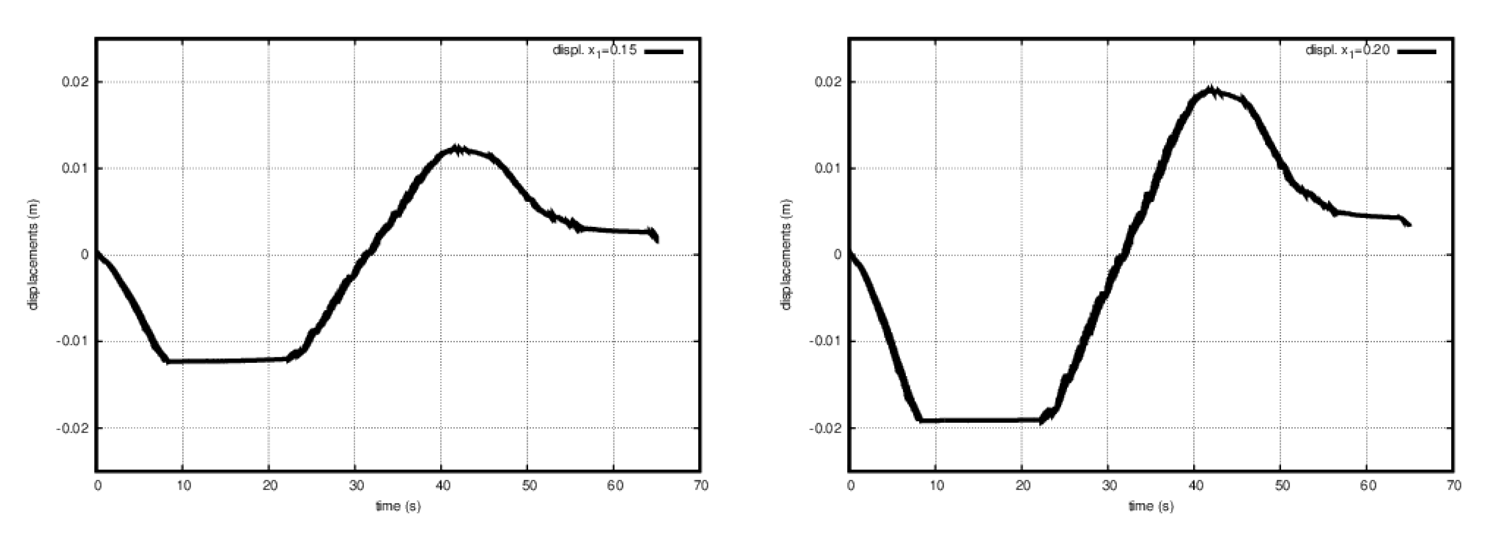
In Figure 2, it can be seen that the slope of the curves was zero when the structure was in contact with the obstacle. The structure traveled down and made contact with the rigid disk from 9 s to 23 s, then it ascended. At 32 s, the position was similar to the undeformed shape, it continued to ascend up to maximal position at 43 s and then descended.
At each time step, we solve the fluid–structure interaction problem iteratively using the fixed point method. At each fixed point iteration, one fluid sub-problem and one structure sub-problem are solved. The number of iterations at each time step gives an indicator of the computational effort. In this simulation, the number of fixed point iterations was less than 5, except for five time steps, where the number was 7, 10 and for three time steps it was 50. Slow convergence of the fixed point method can be explained when the contraction constant of the map was close to 1. Other methods for implicitly solving the fluid–structure interaction problem are Newton or quasi-Newton methods, see [38] for a comparative study.
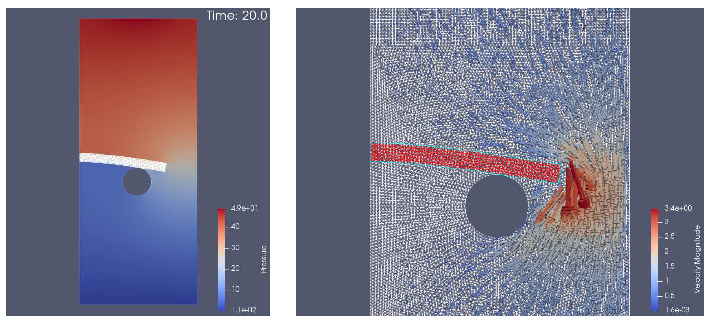
In Figure 3, we show the computed solution at time instant t = 20 s when the structure starts to touch the obstacle. The fluid velocity was maximal near the right end of the structure. In the zone limited by the left side of the fluid domain, the bottom side of the structure and the obstacle, the fluid velocity was very small.
7.2. Numerical Simulation of Valve Dynamics
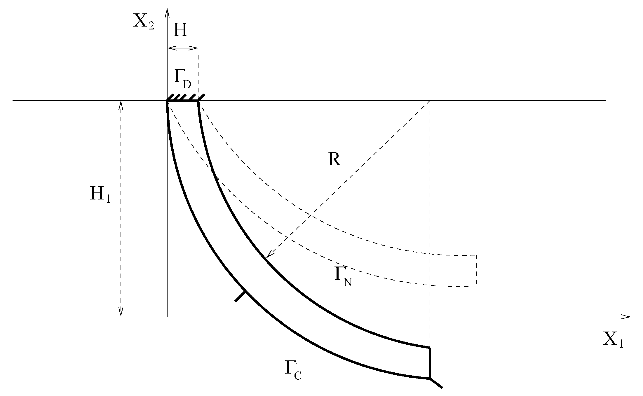
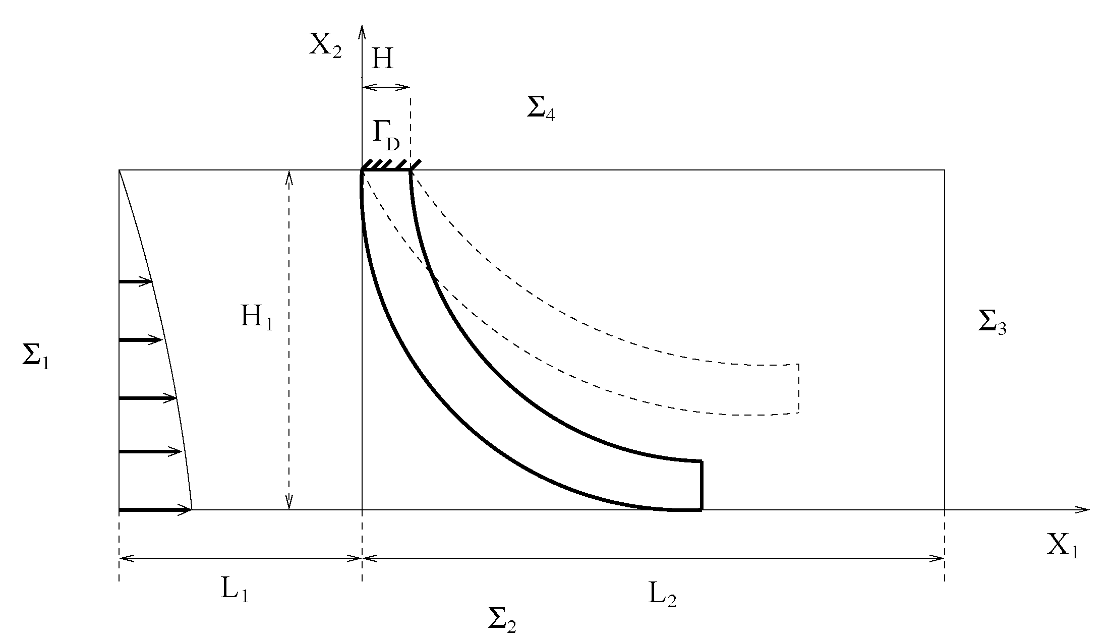
The undeformed structure domain is a quarter of a ring with interior radius , thickness and center , where , see Figure 4. Its boundaries are as follows: ,
and . Let , be the rigid fondation.
The fluid domain is . For the numerical tests, we used the values: , , , see Figure 5.
The mechanical properties of the elastic structure are the following: mass density , Young’s modulus , Poisson’s ratio , applied volume forces on the structure , .
The parameters for the fluid are: mass density , dynamic viscosity , applied volume forces on the fluid , . The inflow velocity profile is where and
with or , and . The boundary conditions for the fluid are as follows: on , on , on , and on with , see Figure 5. The initial conditions are as follows: , . Since, the undeformed structure domain does not satisfy the non-penetration constraint, we solved a steady elasticity contact problem to obtain .
We used a fluid mesh of 13,090 triangles and 6718 vertices, fluid mesh size , a structure mesh of 40 triangles and 42 vertices, structure mesh size , the time step and the number of time steps . The penalization parameter was , the relaxation parameter was set to and for the stopping test . At Step 2, we solved a linear system of dimension 33,244 and at Step 4, we solved a constrained optimization problem of dimension 84, subject to 9 inequalities corresponding to (26) and 4 components were fixed to zero corresponding to (27).
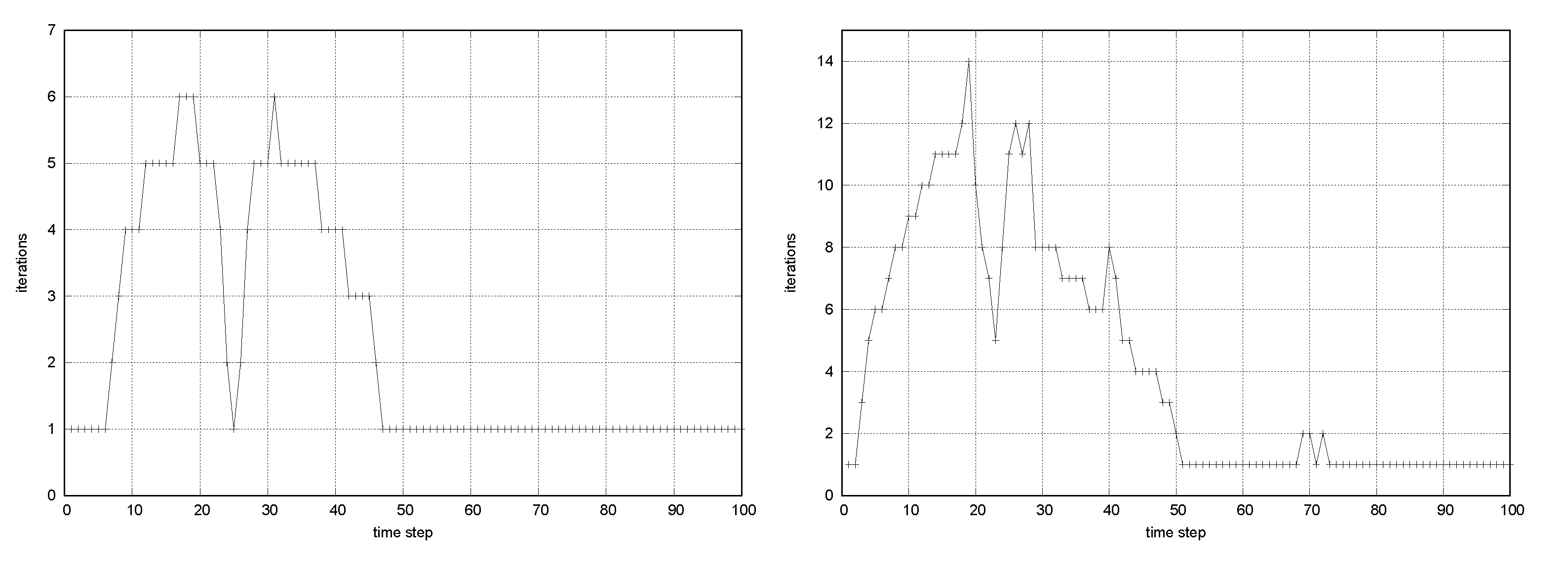
We observe in Figure 6, the number of fixed point iterations at each time step, which proves the efficiency of the method. The structure velocity was near to zero, when the opening of the valve was maximal or when the valve was closed, then only 1–2 iterations were necessary to achieve the convergence. The total computational time was 323 s for and 584 s for .
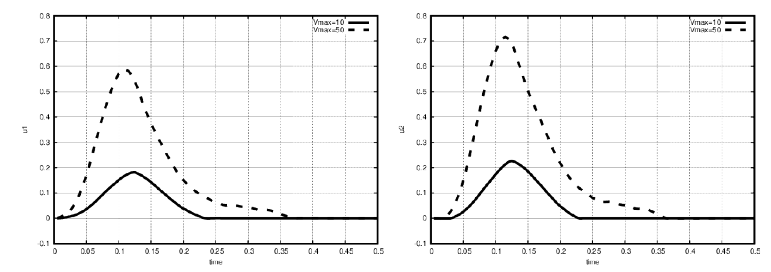
In Figure 7, we plot the horizontal and vertical displacement of the structure tail. We observe in this figure that the valve was closed after about for and after about for .
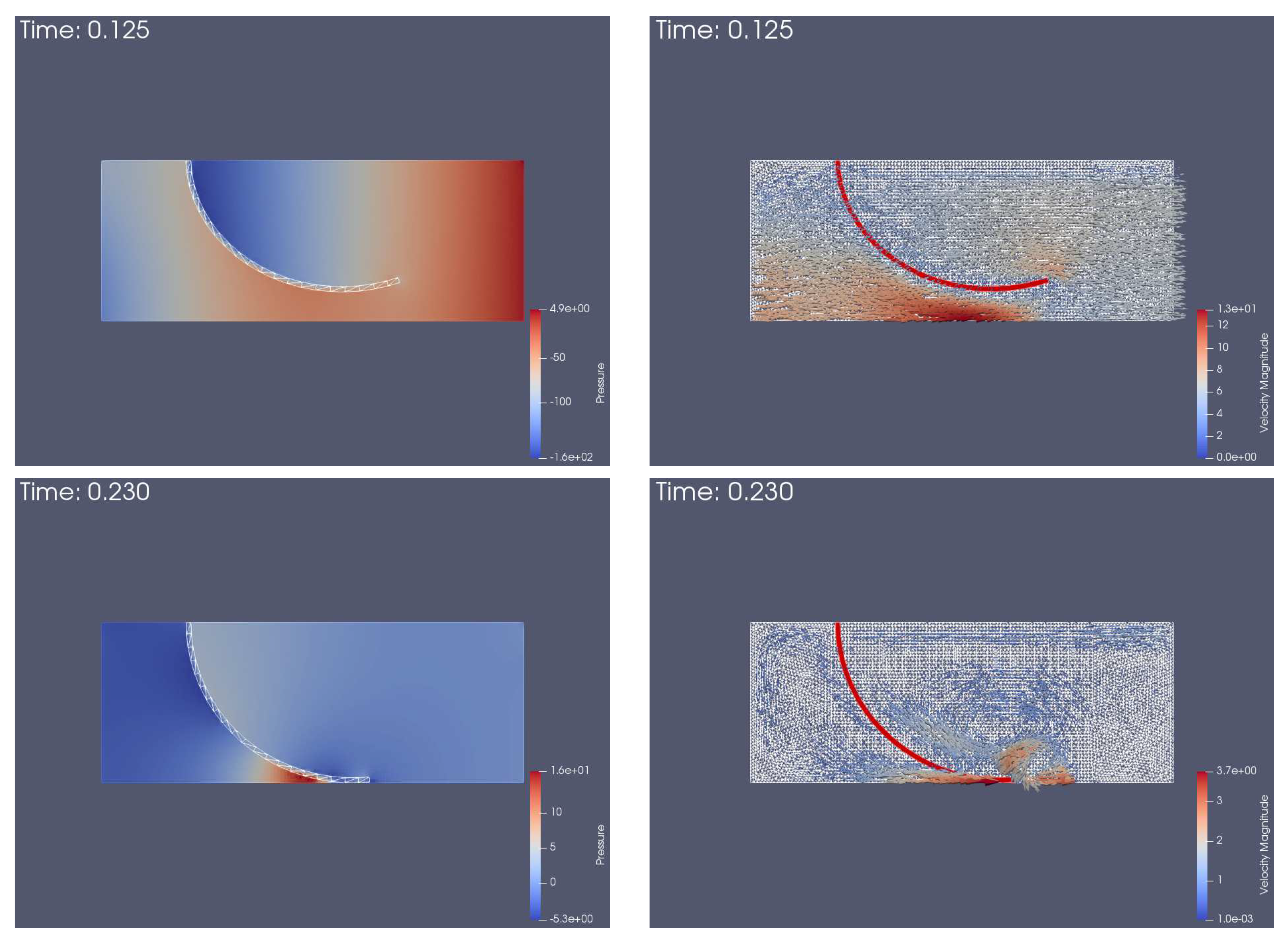
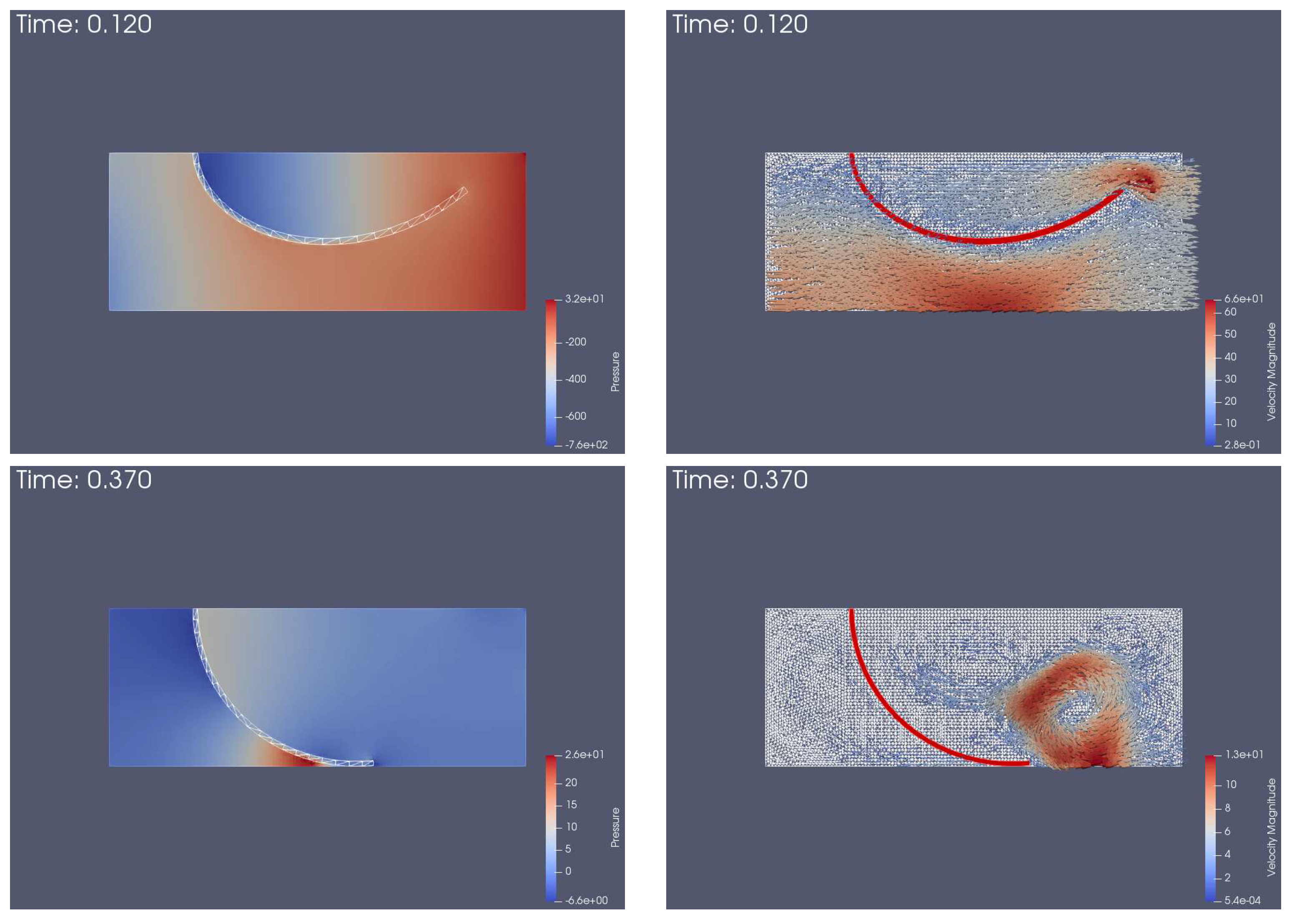
At the initial time, the valve was closed and prestressed, since the undeformed structure domain did not satisfy the non-penetration constraint. It ascended to its highest opening position, see Figure 8 the top images, then the valve descended and made contact with the rigid foundation, see Figure 8 the bottom images, for .
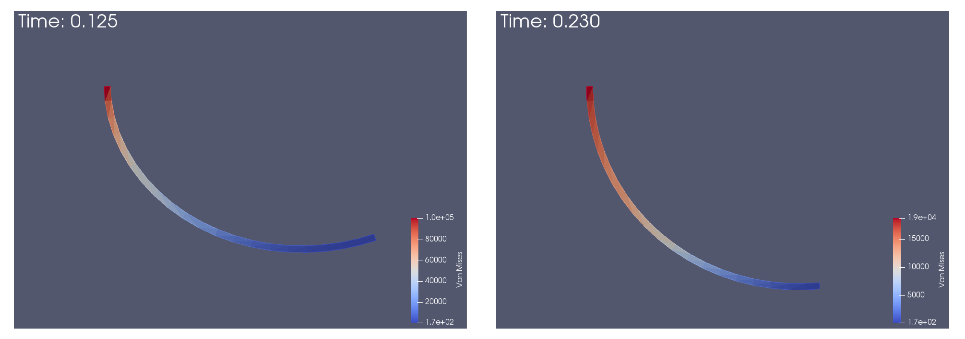
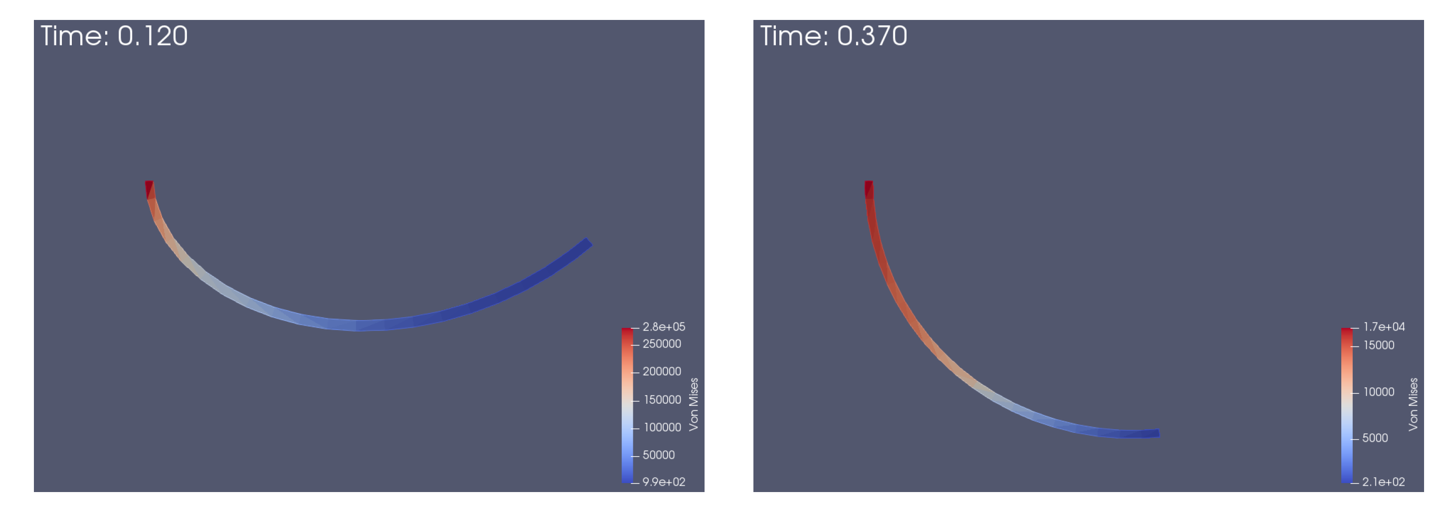
In Figure 9, Von Mises stress distribution in the structure is shown for . We observe that Von Mises stress was larger near to the top fixed boundary even when the valve was in contact with the bottom wall. The reason for this is that the structure was prestressed when the valve was closed. Similar behavior we observe for , in Figure 10 and Figure 11.
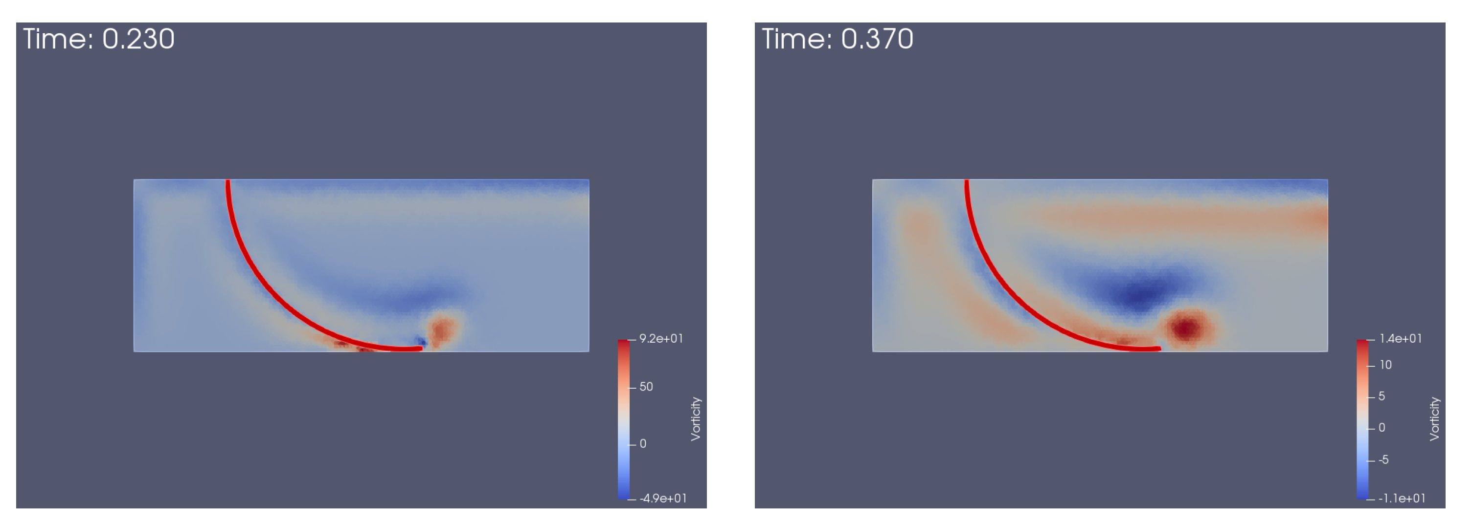
We also observe a vortex downstream of the closed valve, see also Figure 12, where the vorticity is plotted.
The structure deformations are important when and a non-linear model for the elasticity equations could be used.
7.3. Check Valve Interacting with Navier–Stokes Flow
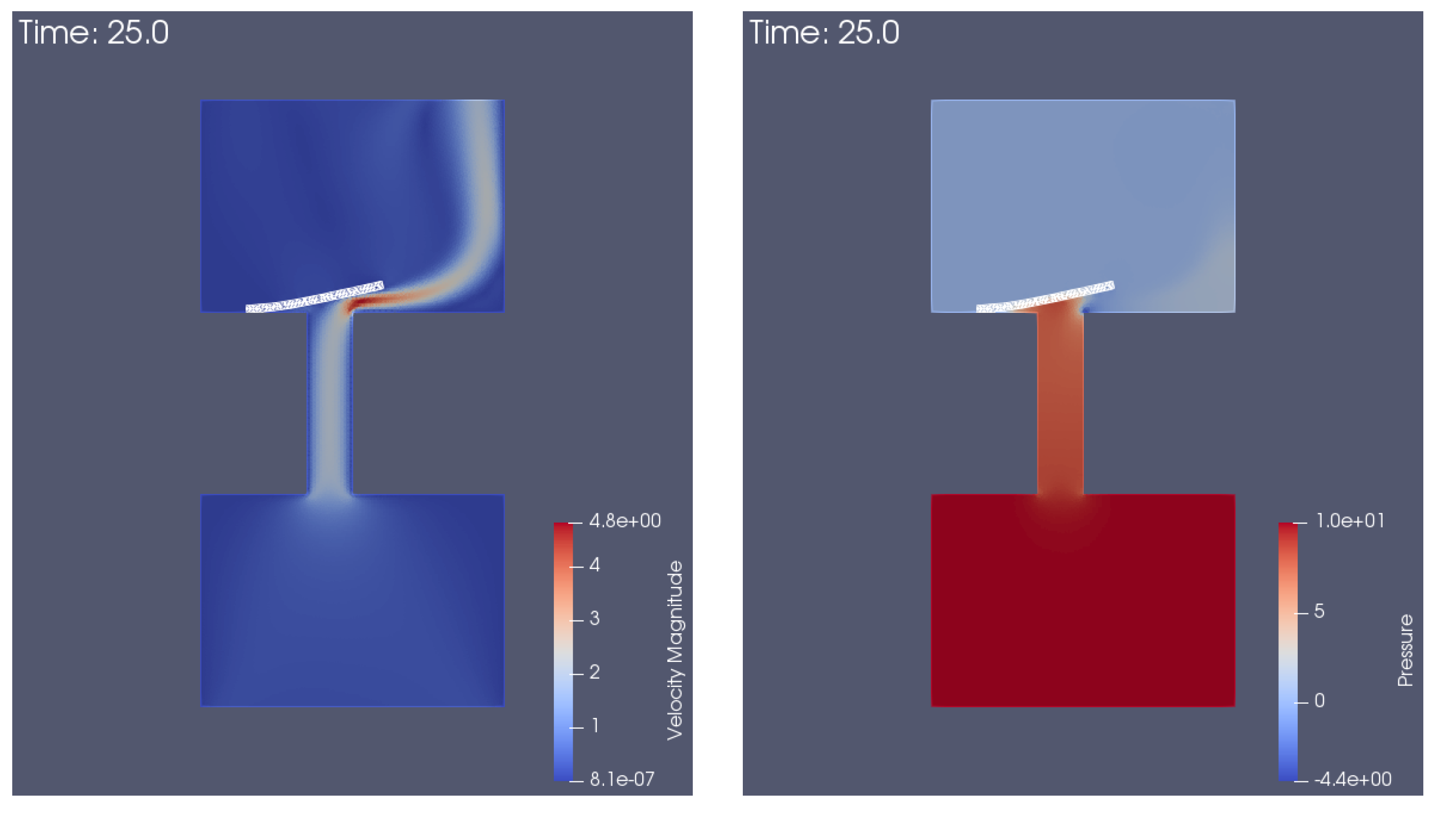
As we seen in Remark 2, the extension from Stokes to Navier–Stokes equations for the fluid is straightforward. Now, we present the numerical results for the check valve problem adapted from [15]. In our case, the fluid is governed by the Navier–Stokes equations but the structure is still governed by the linear elasticity equations.
All the units are derived from centimeter (cm), gram (g), millisecond (ms). The fixed computational fluid domain D was the union of three rectangles: (bottom), (middle) and (top). The mass density of the fluid was , the dynamic viscosity was and the boundary conditions were as follows:
prescribed surface stress at the bottom boundary, do-nothing at the top boundary and non-slip boundary condition otherwise. There were no applied volume forces in fluid.
The undeformed structure domain was a rectangle of thickness and length and the coordinates of the left bottom corner were . The mass density, Young’s modulus, Poisson’s ratio of the structure were as follows: , , , respectively. There were no applied volume forces in structure.
In the paper [15], the structure is modeled with Neo-Hookean material of thickness and . Our technique to compute the forces at the fluid–structure interface using integral over the structure domain requires a structure that is not too thin. For this reason, we used a structure of thickness . A linear model for the structure with gives important displacements, for this reason we worked with .
The fluid mesh had 34,432 triangles and 17,602 vertices, the structure mesh had 156 triangles and 121 vertices, the time step was Δt = 0.05 . The penalization parameter , the relaxation parameter , the parameter for the stopping test was and the finite elements were the same as in the previous simulations.
The contour plots of the velocity and pressure in Figure 13 are very similar to [15]. The maximal velocity magnitude is comparable with in [15] and the minimal pressure was obtained in the right top corner of the middle rectangle of the fluid domain: in our test and in [15].
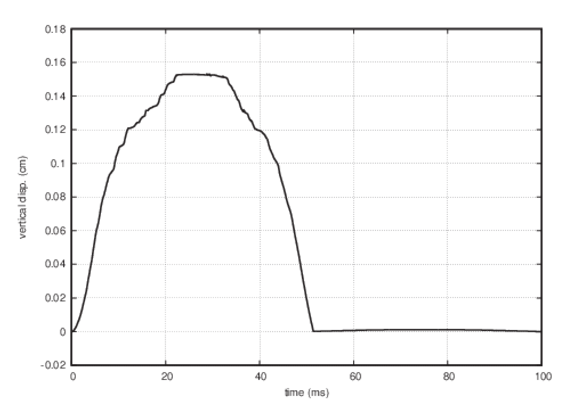
The vertical displacement of the structure tail in Figure 14 is correlated to the surface stress at the inflow (41): the valve ascended to its highest position , then descended and made contact with the rigid obstacle after . The valve was closed in the time interval . One difference from the report of [15], was that in our test, the shape of the vertical displacement of the structure tail did not have two humps in the time interval .
8. Conclusions
We have presented a numerical method for solving by partitioned procedures the dynamic behavior of an elastic thick structure immersed in an incompressible fluid. This method handles the contact between a linear elastic structure and a rigid obstacle. For the fluid flow, the fictitious domain method with penalization was used. The surface forces at the fluid–structure interface were computed using the fluid solution in the structure domain. Numerical tests were presented.
Author Contributions
The authors contributed equally to this work. All authors have read and agreed to the published version of the manuscript.
Funding
This research received no external funding.
Conflicts of Interest
The authors declare no conflict of interest.
References
- Quarteroni, A.; Formaggia, L. Mathematical modelling and numerical simulation of the cardiovascular system. In Handbook of Numerical Analysis; Ciarlet, P.G., Ed.; North-Holland: Amsterdam, The Netherlands, 2004; Volume XII, pp. 3–127. [Google Scholar]
- Tezduyar, T.E.; Sathe, S. Modelling of fluid-structure interactions with the space-time finite elements: Solution techniques. Int. J. Num. Meth. Fluids 2007, 54, 855–900. [Google Scholar] [CrossRef]
- Peskin, C.S. The immersed boundary method. Acta Numer. 2002, 11, 479–517. [Google Scholar] [CrossRef] [Green Version]
- Boffi, D.; Gastaldi, L.; Heltai, L.; Peskin, C. On the hyper-elastic formulation of the immersed boundary method. Comput. Methods Appl. Mech. Engrg. 2008, 197, 2210–2231. [Google Scholar] [CrossRef]
- Glowinsk, R.; Hesla, T.I.; Joseph, D.; Pan, T.; Périaux, J. A distributed Lagrange multiplier/fictitious domain method for the simulation of flow around moving rigid bodies: Application to particulate flow. Comput. Methods Appl. Mech. Engrg. 2000, 184, 241–267. [Google Scholar] [CrossRef]
- Boffi, D.; Gastaldi, L. A fictitious domain approach with Lagrange multiplier for fluid-structure interactions. Numer. Math. 2017, 135, 711–732. [Google Scholar] [CrossRef] [Green Version]
- Bost, C.; Cottet, G.-H.; Maitre, E. Convergence analysis of a penalization method for the three-dimensional motion of a rigid body in an incompressible viscous fluid. SIAM J. Numer. Anal. 2010, 48, 1313–1337. [Google Scholar] [CrossRef]
- Court, S.; Fournié, M.; Lozinski, A. A fictitious domain approach for fluid-structure interactions based on the extended finite element method. ESAIM Proc. Surv. 2014, 45, 308–317. [Google Scholar] [CrossRef]
- Alauzet, F.; Fabrèges, B.; Fernández, M.A.; Landajuela, M. Nitsche-XFEM for the coupling of an incompressible fluid with immersed thin-walled structures. Comput. Methods Appl. Mech. Engrg. 2016, 301, 300–335. [Google Scholar] [CrossRef] [Green Version]
- Dos Santos, N.; Gerbeau, J.-F.; Bourgat, J.-F. A partitioned fluid-structure algorithm for elastic thin valves with contact. Comput. Methods Appl. Mech. Engrg. 2008, 197, 1750–1761. [Google Scholar] [CrossRef] [Green Version]
- Astorino, M.; Gerbeau, J.-F.; Pantz, O.; Traoré, K.-F. Fluid-structure interaction and multi-body contact: Application to aortic valves. Comput. Methods Appl. Mech. Engrg. 2009, 198, 3603–3612. [Google Scholar] [CrossRef] [Green Version]
- Mayer, U.M.; Popp, A.; Gerstenberger, A.; Wall, W. 3D fluid-structure-contact interaction based on a combined XFEM FSI and dual mortar contact approach. Comput. Mech. 2010, 46, 53–67. [Google Scholar] [CrossRef]
- Kamensky, D.; Hsu, M.-C.; Schillinger, D.; Evans, J.A.; Aggarwal, A.; Bazilevs, Y.; Sacks, M.S.; Hughes, T.J.R. An immersogeometric variational framework for fluid-structure interaction: Application to bioprosthetic heart valves. Comput. Methods Appl. Mech. Engrg. 2015, 284, 1005–1053. [Google Scholar] [CrossRef] [PubMed] [Green Version]
- Hecht, F.; Pironneau, O. An energy stable monolithic Eulerian fluid-structure finite element method. Int. J. Numer. Methods Fluids 2017, 85, 430–446. [Google Scholar] [CrossRef]
- Kadapa, C.; Dettmer, W.G.; Peric, D. A stabilised immersed framework on hierarchical b-spline grids for fluid-flexible structure interaction with solid-solid contact. Comput. Methods Appl. Mech. Engrg. 2018, 335, 472–489. [Google Scholar] [CrossRef] [Green Version]
- Ager, C.; Schott, B.; Vuong, A.-T.; Popp, A.; Wall, W.A. A consistent approach for fluid-structure-contact interaction based on a porous flow model for rough surface contact. Int. J. Numer. Methods Eng. 2019, 119, 1345–1378. [Google Scholar] [CrossRef] [Green Version]
- Burman, E.; Fernández, M.A.; Frei, S. A Nitsche-based formulation for fluid-structure interactions with contact. ESAIM M2AN 2020, 54, 531–564. [Google Scholar] [CrossRef]
- Yakhlef, O.; Murea, C.M. Numerical procedure for fluid-structure interaction with the structure displacements limited by a rigid obstacle. Appl. Comput. Mech. 2017, 11, 91–104. [Google Scholar] [CrossRef]
- Halanay, A.; Murea, C.M.; Tiba, D. Existence and approximation for a steady fluid-structure interaction problem using fictitious domain approach with penalization. Ann. Acad. Rom. Sci. Ser. Math. Appl. 2013, 5, 120–147. [Google Scholar]
- Halanay, A.; Murea, C.M.; Tiba, D. Existence of a steady flow of Stokes fluid past a linear elastic structure using fictitious domain. J. Math. Fluid Mech. 2016, 18, 397–413. [Google Scholar] [CrossRef]
- Ciarlet, P.G. Mathematical Elasticity. Volume 1: Three Dimensional Elasticity; Elsevier: Amsterdam, The Netherlands, 2004. [Google Scholar]
- Halanay, A.; Murea, C.M.; Tiba, D. Extension theorems related to a fluid-structure interaction problem. Bull. Math. Soc. Sci. Math. Roum. 2018, 61, 417–437. [Google Scholar]
- Halanay, A.; Murea, C.M. Uniform Estimation of a Constant Issued from a Fluid-Structure Interaction Problem. In System Modeling and Optimization; IFIP Advances in Information and Communication Technology; Bociu, L., Désidéri, J.-A., Habbal, A., Eds.; Springer: Berlin, Germany, 2016; Volume 494, pp. 292–301. [Google Scholar]
- Kikuchi, N.; Oden, J.T. Contact Problems in Elasticity: A Study of Variational Inequalities and Finite Element Methods; SIAM Studies in Applied Mathematics; Society for Industrial and Applied Mathematics (SIAM): Philadelphia, PA, USA, 1988; Volume 8. [Google Scholar]
- Eck, C.; Jarusek, J.; Krbec, M. Unilateral Contact Problems. Variational Methods and Existence Theorems; Chapman and Hall/CRC: Boca Raton, FL, USA, 2005. [Google Scholar]
- Duvaut, G.; Lions, J.-L. Les inÉquations en mÉcanique et en Physique; Travaux et Recherches Mathématiques; Dunod: Paris, France, 1972; Volume 21. [Google Scholar]
- Lebeau, G.; Schatzman, M. A wave problem in a half-space with a unilateral constraint at the boundary. J. Differ. Equ. 1984, 53, 309–361. [Google Scholar] [CrossRef] [Green Version]
- Chau, O.; Shillor, M.; Sofonea, M. Dynamic frictionless contact with adhesion. Z. Angew. Math. Phys. 2004, 55, 32–47. [Google Scholar] [CrossRef]
- Eck, C.; Jarusek, J.; Sofonea, M. A dynamic elastic-visco-plastic unilateral contact problem with normal damped response and Coulomb friction. Eur. J. Appl. Math. 2010, 21, 229–251. [Google Scholar] [CrossRef]
- Doyen, D.; Ern, A.; Piperno, S. Time-integration schemes for the finite element dynamic Signorini problem. SIAM J. Sci. Comput. 2011, 33, 223–249. [Google Scholar] [CrossRef] [Green Version]
- Krause, R.; Walloth, M. Presentation and comparison of selected algorithms for dynamic contact based on the Newmark scheme. Appl. Numer. Math. 2012, 62, 1393–1410. [Google Scholar] [CrossRef]
- Lewy, H. On the coincidence set in variational inequality. J. Differ. Geom. 1971, 6, 497–501. [Google Scholar] [CrossRef]
- Kinderlehrer, D.; Stampacchia, G. An Introduction to Variational Inequalities and Their Applications; Reprint of the 1980 Original. Classics in Applied Mathematics; Society for Industrial and Applied Mathematics (SIAM): Philadelphia, PA, USA, 2000; Volume 31. [Google Scholar]
- Rodrigues, J.F. Obstacle Problems in Mathematical Physics; North-Holland Publishing Co.: Amsterdam, The Netherlands, 1987. [Google Scholar]
- Dautray, R.; Lions, J.-L. Analyse Mathématique et Calcul Numérique pour les Sciences et les Techniques; Masson: Paris, France, 1988; Volume 4. [Google Scholar]
- Boyer, F.; Fabrie, P. Mathematical Tools for the Study of the Incompressible Navier-Stokes Equations and Related Models; Applied Mathematical Sciences; Springer: New York, NY, USA, 2013; Volume 183. [Google Scholar]
- Hecht, F. New development in FreeFem++. J. Numer. Math. 2012, 20, 251–265. [Google Scholar] [CrossRef]
- Murea, C.M. Numerical simulation of a pulsatile flow through a flexible channel. ESAIM Math. Model. Numer. Anal. 2006, 40, 1101–1125. [Google Scholar] [CrossRef]
Figure 1.
The undeformed structure domain (continuous line) and deformed structure domain (pointed line) in contact with the obstacle.
Figure 1.
The undeformed structure domain (continuous line) and deformed structure domain (pointed line) in contact with the obstacle.

Figure 2.
Time history of the vertical displacement of two points at for (left) and (right).

Figure 3.
Computed solution at time instant t = 20 s: pressure (left) and zoom of velocity (right).

Figure 4.
Undeformed structure domain does not satisfy the non-penetration constraint.

Figure 5.
The geometrical configuration of fluid–structure.

Figure 6.
Time history of iterations number to obtain the convergence at each time step for (left) and (right).
Figure 6.
Time history of iterations number to obtain the convergence at each time step for (left) and (right).

Figure 7.
The relatively displacement by rapport of the initial configuration of the bottom corner of the tail segment of the structure: horizontal (left) and vertical (right).
Figure 7.
The relatively displacement by rapport of the initial configuration of the bottom corner of the tail segment of the structure: horizontal (left) and vertical (right).

Figure 8.
Computed solution for , pressure (left) and velocity (right): when the valve was at the highest position t = 0.125 s (top) and when the valve made contact with the foundation t = 0.230 s (bottom).
Figure 8.
Computed solution for , pressure (left) and velocity (right): when the valve was at the highest position t = 0.125 s (top) and when the valve made contact with the foundation t = 0.230 s (bottom).

Figure 9.
Von Mises stress distribution in the structure for .

Figure 10.
Computed solution for , pressure (left) and velocity (right): when the valve was at the highest position t = 0.120 s (top) and when the valve made contact with the foundation t = 0.370 s (bottom).
Figure 10.
Computed solution for , pressure (left) and velocity (right): when the valve was at the highest position t = 0.120 s (top) and when the valve made contact with the foundation t = 0.370 s (bottom).

Figure 11.
Von Mises stress distribution in the structure .

Figure 12.
Vorticity distribution when the valve starts to be in contact with the foundation for (left) and (right).
Figure 12.
Vorticity distribution when the valve starts to be in contact with the foundation for (left) and (right).

Figure 13.
Velocity magnitude (left) and pressure (right) of the fluid at t = 25 ms, when the structure is at the highest position.
Figure 13.
Velocity magnitude (left) and pressure (right) of the fluid at t = 25 ms, when the structure is at the highest position.

Figure 14.
Vertical displacement of the right bottom corner of the structure.

Publisher’s Note: MDPI stays neutral with regard to jurisdictional claims in published maps and institutional affiliations. |
© 2021 by the authors. Licensee MDPI, Basel, Switzerland. This article is an open access article distributed under the terms and conditions of the Creative Commons Attribution (CC BY) license (http://creativecommons.org/licenses/by/4.0/).
Share and Cite
MDPI and ACS Style
Yakhlef, O.; Murea, C.M. Numerical Simulation of Dynamic Fluid-Structure Interaction with Elastic Structure–Rigid Obstacle Contact. Fluids 2021, 6, 51. https://0-doi-org.brum.beds.ac.uk/10.3390/fluids6020051
AMA Style
Yakhlef O, Murea CM. Numerical Simulation of Dynamic Fluid-Structure Interaction with Elastic Structure–Rigid Obstacle Contact. Fluids. 2021; 6(2):51. https://0-doi-org.brum.beds.ac.uk/10.3390/fluids6020051
Chicago/Turabian StyleYakhlef, Othman, and Cornel Marius Murea. 2021. "Numerical Simulation of Dynamic Fluid-Structure Interaction with Elastic Structure–Rigid Obstacle Contact" Fluids 6, no. 2: 51. https://0-doi-org.brum.beds.ac.uk/10.3390/fluids6020051