Direct Numerical Simulation of Sediment Transport in Turbulent Open Channel Flow Using the Lattice Boltzmann Method

Abstract

The lattice Boltzmann method is employed to conduct direct numerical simulations of turbulent open channel flows with the presence of finite-size spherical sediment particles. The uniform particles have a diameter of approximately 18 wall units and a density of ${\rho }_p=2.65{\rho }_f$, where ${\rho }_p$ and ${\rho }_f$ are the particle and fluid densities, respectively. Three low particle volume fractions $\varphi =0.11\%$, 0.22%, and 0.44% are used to investigate the particle-turbulence interactions. Simulation results indicate that particles are found to result in a more isotropic distribution of fluid turbulent kinetic energy (TKE) among different velocity components, and a more homogeneous distribution of the fluid TKE in the wall-normal direction. Particles tend to accumulate in the near-wall region due to the settling effect and they preferentially reside in low-speed streaks. The vertical particle volume fraction profiles are self-similar when normalized by the total particle volume fractions. Moreover, several typical transport modes of the sediment particles, such as resuspension, saltation, and rolling, are captured by tracking the trajectories of particles. Finally, the vertical profiles of particle concentration are shown to be consistent with a kinetic model.

1. Introduction

Sediment transport is common in rivers, lakes, estuaries, and seacoasts. In these hydraulic systems, the flow regime is turbulent. Both the dynamics of the sediments and the properties of the turbulent flows could be affected by sediment-turbulence interactions. Therefore, gaining a deeper comprehension of sediment-turbulence interactions can help us better understand the transport phenomenon.

In the past, many experimental measurements were conducted to investigate sediment-turbulence interactions. Rashidi et al. [1] experimentally investigated a Plexiglas rectangular channel with solid particles of various sizes. They found that large particles (with a mean diameter at 1100 µm) increased the Reynolds stress and turbulence intensity, while small particles (with a mean diameter at 120 µm) led to opposite modulations. The particle-fluid interactions in an open channel turbulent boundary layer were explored by Baker and Coletti [2]. The spherical hydrogel particles had a diameter of approximately 9% of the channel depth and were slightly denser than the fluid. Their results showed that the turbulent activities were damped near the wall by the particles; however, in the outer region of the flow, the sweep and ejection motions of the turbulence were enhanced. Righetti and Romano [3] studied a closed-circuit rectangular Plexiglas open channel with glass spheres (${\rho }_p/{\rho }_f=2.6$) of two different sizes (mean diameters at 100 µm and 200 µm). They reported that the particle mean streamwise velocity was smaller than its fluid counterpart except for particles that resided very close to the wall. The inception motion of sediment particles (mean diameter ranges from 20.8 mm to 83.2 mm) in a recirculating flume was examined by Dwivedi et al. [4], and their results revealed that the inception was highly correlated with strong sweep flow structures for both shielded and exposed particles.

Besides the experimental studies, numerical simulations of sediment-laden flows also attract increasing attention. In principle, the transport of particles in a fluid flow could be modeled by three approaches: Eulerian method [5], Lagrangian point-particle method [6], and interface-resolved simulation [7]. The Eulerian method treats the particles as a continuum and the particle-fluid interactions are described by drag force correlations. This method fails to fully consider the particle-particle interactions and cannot track the movement of each particle. The Lagrangian point-particle method is applicable to situations where the particle size is much smaller than the Kolmogorov length scale and particles are dilute. This method assumes particles are point masses without volume. Drag force correction models are also needed to account for particle-fluid interactions. The interface-resolved simulation is the only appropriate method when particle sizes are comparable to or larger than the Kolmogorov length scale. This method considers the particle finite-size effect and resolves directly the disturbance flows around each particle. Consequently, the particle-turbulence interactions are fully resolved by the interface-resolved direct numerical simulations (IRDNS).

As one of the first simulations of the IRDNS, Pan and Banerjee [8] investigated a turbulent open channel flow seeded with finite-size particles of different sizes. They found that the ejection-sweep cycles were affected primarily through the suppression of sweeps by the smaller particles and enhancement of sweep activity by the larger particles. Simulations of horizontal open channel flow laden with finite-size heavy particles at a low solid volume fraction were performed by Kidanemariam et al. [9], and their results implied that the particles formed elongated streamwise structures, resembling aligned chains. The results of Ji et al. [10] indicated that the particle movements were closely related to the turbulent events and the protruding bed roughness can undermine the near-wall streaky structures. In the investigations of Yousefi et al. [11], the dynamics of a single sediment particle in a turbulent open channel flow over a fixed porous bed was explored. They reported that particles could resuspend or saltate if the Galileo number $Ga$ was less than 150, while particles tend to only roll on the bed if $Ga$ was greater than 150. Here, the Galileo number is defined as $Ga=\sqrt{({\rho }_p/{\rho }_f-1)g{D}^3}/\nu$, where g is the gravitational acceleration, D is the particle diameter, and $\nu$ is the fluid kinematic viscosity. $Ga$ is related to the ratio of the particle effective gravity to the viscous force. Derksen et al. [12] studied turbulent open channel flows laden with solid particles. Their results showed that the particle motion was strongly related to the strength of the turbulent fluctuations. Although these previous studies have provided some insight into understanding sediment-turbulence interactions, the problem is still poorly understand, and many questions remain unanswered. For example, how do heavy particles modulate the turbulent flow? How does turbulence affect the dynamics of individual sediment particles near the bed surface? These questions motivate us to conduct the present study.

On the other hand, most of these aforementioned IRDNS of sediment-laden flows are based on directly solving the Navier–Stokes equations. Compared to the conventional N-S solvers, the lattice Boltzmann method (LBM) has bettter flexibility in treating the boundary conditions. Specifically, using the interpolated bounce-back (IBB) schemes to treat the no-slip boundary condition can easily ensure a second-order accuracy, which has been shown to result in more accurate results in particulate flow simulations than the commonly used diffused-interface immersed boundary method (IBM) [13]. This relatively new approach has been convincingly validated and benchmarked in various particle-laden turbulent flows, such as homogeneous isotropic flows [14], pipe flows [15], and channel flows [16]. In light of these previous studies, we chose the IBB-based LBM as our numerical method to conduct IRDNS to investigate sediment-turbulence interactions in the present study.

The remainder of this paper is organized as follows. Section 2 briefly introduces LBM and its treatments of finite-size particles. In Section 3, simulation settings and code validation are given. The fluid statistics, flow structures, particle statistics, and particle dynamics are analyzed in Section 4. Finally, the major conclusions are recapitulated in Section 5.

2. Numerical Methodology

2.1. Problem Description

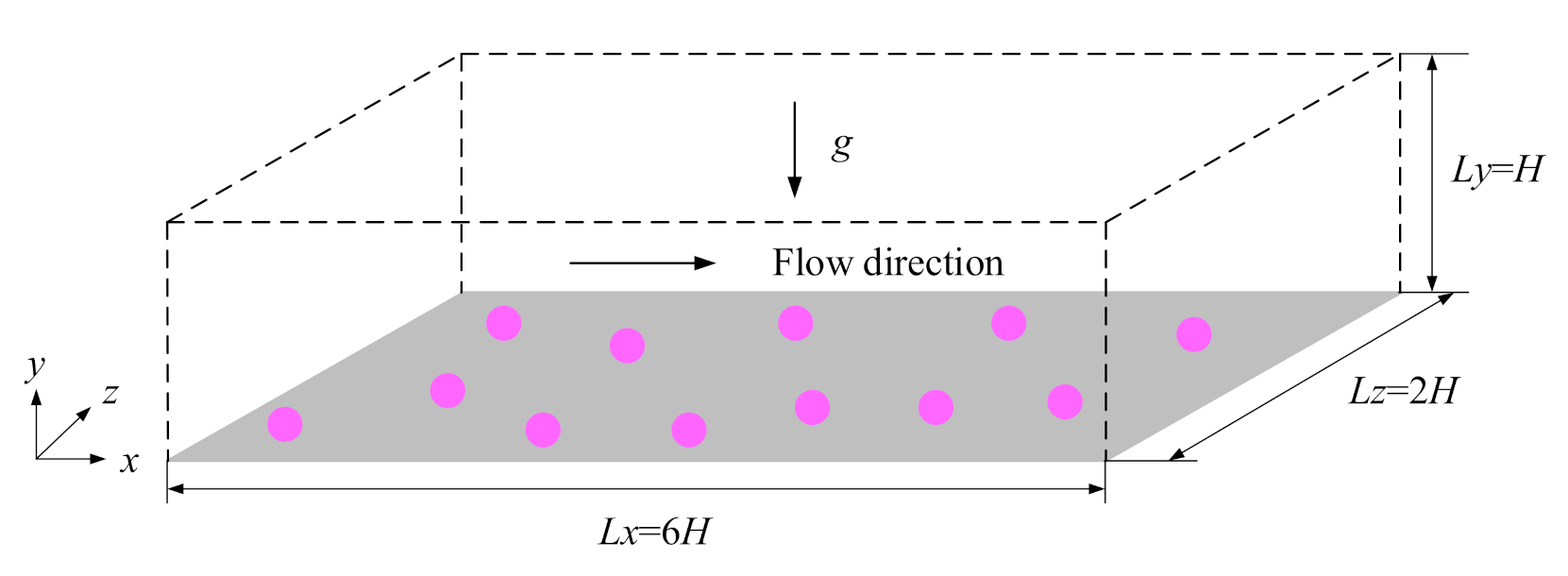
In this work, a horizontal turbulent open channel flow seeded with rigid, spherical, and finite-size sediment particles is investigated. As shown in Figure 1, spatial coordinates x, y, and z stand for the streamwise, wall-normal, and spanwise directions, respectively. The channel has a size of $L_x\times L_y\times L_z=6H\times H\times 2H$, where H is the channel height. Mean flow and gravitational force are directed in the positive x and negative y directions, respectively. Periodic boundary conditions are applied in the streamwise and spanwise directions. A no-slip boundary condition is imposed at the bottom wall ($y=0$) and free-slip condition [17] is assumed at the top boundary ($y=H$). The friction Reynolds number is set to be $R{e}_{\tau }=u_{\tau }H/\nu =180$, where $u_{\tau }=\sqrt{〈{\tau }_w〉/{\rho }_f}$ is the wall friction velocity and $〈{\tau }_w〉$ is the time-averaged wall shear stress.

The normalized diameter of the finite-size sediment particles is $D/H=0.1$. The particle-to-fluid density ratio is ${\rho }_p/{\rho }_f=2.65$, which is a typical density ratio between sediment and water in reality (i.e., ${\rho }_p=2650$ kg/m${}^3$, ${\rho }_f=1000$ kg/m${}^3$) [18]. The Shields number is defined as $\Theta ={\rho }_f{u}_{\tau }^2/\left[({\rho }_p-{\rho }_f)gD\right]$, indicating the ratio of fluid shear force on the particle to the effective gravitational force. Here we set $\Theta =0.5$, a value of relevance to sediment transport [19]. A small Shields number implies that particles will settle to the bottom under gravity, and a large Shields number implies that turbulent motion can lift off and suspend particles. In this study, one single-phase case and three sediment-laden cases with different particle volume fractions (i.e., $\varphi =0.11\%$, 0.22%, and 0.44%) are simulated. When sediment volume fractions are high, sediment particles would form a sediment layer on the bottom channel wall and serve as a rough surface. Studies of dense sediment-laden turbulent channel flows have been reported by Ji et al. [10] and Shao et al. [20]. Here we focus on sediment-turbulence interactions with relatively low sediment volume fractions as a supplement of those previous studies. As the driving force per unit volume is fixed in all cases, low sediment volume fractions are chosen to avoid introducing too large attenuation to the turbulent kinetic energy, as reported by Peng et al. [16].

2.2. Flow Solver

LBM is applied to conduct DNS of the turbulent open channel flow in the current simulation. Unlike the traditional computational fluid dynamic approaches based on directly solving the continuum N-S equations, LBM solves the evolution of mesoscopic fluid-particle distribution functions. Following our previous study [13], the multiple-relaxation time (MRT) LBM algorithm is chosen due to its better numerical stability compared to the single-relaxation time (SRT) LBM. The governing equation of MRT-LBM is expressed as:

$$\begin{array}{c}\hfill \mathit{f}(\mathit{x}+{\mathit{c}}_i\Delta t,t+\Delta t)-\mathit{f}(\mathit{x},t)=-{\mathit{M}}^{-1}\mathit{S}[\mathit{m}(\mathit{x},t)-{\mathit{m}}^{eq}(\mathit{x},t)]+{\mathit{M}}^{-1}\Psi ,\end{array}$$

(1)

where $\mathit{f}$ is the distribution function, $\mathit{x}$ is the spatial location, ${\mathit{c}}_i$ represents the discrete velocities, $\Delta t$ is the time step, $\mathit{M}$ is the transformation matrix that converts the distribution function $\mathit{f}$ from the velocity space to the moment space $\mathit{m}$, namely, $\mathit{m}=\mathit{M}\mathit{f}$, $\mathit{f}={\mathit{M}}^{-1}\mathit{m}$, $\mathit{S}$ is a diagonal matrix that contains relaxation parameters, ${\mathit{m}}^{eq}$ is the equilibrium moments, ${\mathit{M}}^{-1}\Psi$ represents the effect of external body force, and $\Psi$ denotes the mesoscopic force in the moment space.

The D3Q19 (three-dimensional lattice with 19 discrete velocities) model was most frequently used in the previous studies of particle-laden turbulent flows [14,21]. However, in the present work, the D3Q27 (three-dimensional lattice with 27 discrete velocities) model is adopted because of its better numerical stability [13]. The hydrodynamic variables, such as the local density fluctuation $\delta \rho$, pressure p, and momentum ${\rho }_0\mathit{u}$, are calculated from the moments of the distribution function $\mathit{f}$, as:

$$\delta \rho =\sum _{i=0}^{26}{f}_i,p=\delta \rho c_s^2,{\rho }_0\mathit{u}=\sum _{i=0}^{26}{f}_i{\mathit{c}}_i+\frac{1}{2}\mathit{F}\Delta t,$$

(2)

where, in the lattice units, $c_s=1/\sqrt{3}$ is the speed of the sound for the D3Q27 model, ${\rho }_0$=1 is the background density, $\mathit{u}$ is the macroscopic fluid velocity, and $\mathit{F}$ is the external body force. More detailed information about the D3Q27 MRT-LBM algorithm can be found in the work of Ref. [13].

2.3. Treatments of Particle Interface

In the LBM framework, the diffused-interface immersed boundary method (DI-IBM) and the interpolated bounce-back (IBB) scheme are two major methods used to treat the no-slip boundary condition on the moving particle surfaces. In general, DI-IBM has first-order accuracy while the IBB scheme has second-order accuracy, but the former usually yields better numerical stability [22].

In this study, the quadratic IBB scheme [23] is chosen as the default algorithm to implement the no-slip boundary condition on the particle surfaces. This scheme can guarantee the velocity field to be a second-order accuracy. The main idea of the IBB scheme is that the unknown distribution functions at boundary grid points are directly constructed based on the known ones, so that the no-slip velocity constraints can be satisfied. In order to handle the quadratic IBB scheme, at least two fluid grid points are needed. In the situations where two particles are very close to each other or a particle moves very close to the channel wall, the number of grid points in the gap becomes insufficient for the quadratic interpolation. When these scenarios occur, the linear IBB scheme [23] and the single-node IBB scheme [24] are used. These two schemes also ensure second-order accuracy in boundary treatment. During the interpolation process, the Galilean invariant momentum exchange method [25] is applied to evaluate the hydrodynamic forces and torques acting on particles. When a particle moves to a new position, some previous solid nodes could turn into fluid nodes, and the distribution functions at these uncovered nodes need to be initialized. In the present simulation, a refilling scheme referred to as “equilibrium distribution + non-equilibrium correction” [26] is adopted. The numerical accuracy and stability of the aforementioned schemes have been validated in several particle-laden turbulent flow problems [13].

2.4. Treatments of Particle Movements

When the gap between two particles, or between a particle and the channel wall, gets very narrow, the hydrodynamic interactions between the two solid objects are no longer fully resolved. In these circumstances, a lubrication correction model [27] is introduced to handle the unresolved short-range interactions. The expression of the lubrication model is given as:

$$\begin{array}{c}\hfill {\mathit{F}}_{ij}=-6\pi \mu R[\lambda \left(ϵ\right)-\lambda \left({ϵ}_0\right)]{\mathit{U}}_n,\end{array}$$

(3)

where ${\mathit{F}}_{ij}$ is the lubrication force acting on the ith particle due to the presence of the jth particle, $\mu$ is the fluid dynamic viscosity, R is the particle radius, $ϵ=(\delta -R)/R$ is the ratio of the gap width and the particle radius, $\delta$ is the distance between two approaching particles, ${ϵ}_0$ is the gap threshold value, and ${\mathit{U}}_n$ is half of the longitudinal velocity of the ith particle relative to the jth particle. For particle-particle interactions, $\lambda$ is defined as:

$$\lambda \left(ϵ\right)=\frac{1}{2ϵ}-\frac{9}{20}lnϵ-\frac{3}{56}ϵlnϵ+1.346.$$

(4)

While for particle-wall interactions, $\lambda$ is defined as:

$$\lambda \left(ϵ\right)=\frac{1}{ϵ}-\frac{1}{5}lnϵ-\frac{1}{21}ϵlnϵ+0.9713.$$

(5)

When two solid objects are in physical contact, the soft-sphere collision model [28] is employed to model the collision forces. This model allows particles to have slight overlap and it is intrinsically a spring-dashpot system. The collision force predicted by this soft-sphere model is written as:

$${\mathit{F}}_{ssc}=(-k_n\zeta -{\beta }_n{U}_n){\mathit{n}}_{ij},$$

(6)

$$k_n=\frac{m_e[{\pi }^2+{\left(ln{e}_d\right)}^2]}{{(N_c\Delta t)}^2},{\beta }_n=-\frac{2m_{e}ln{e}_d}{N_c\Delta t},$$

(7)

where ${\mathit{F}}_{ssc}$ is the contact collision force, $k_n$ is the stiffness parameter, $\zeta$ is the overlap distance, ${\beta }_n$ is the damping coefficient, $U_n$ is the magnitude of ${\mathit{U}}_n$, and ${\mathit{n}}_{ij}$ is the unit vector pointing from the jth particle to the ith particle. $m_e$ is the effective mass involved in the collision, $m_e=1/(1/m_i+1/m_j)$ for particle-particle collisions, and $m_e=m$ for particle-wall collisions. $e_d$ is the dry collision coefficient, it is set to be 0.97 [11]. $N_c\Delta t$ is the collision duration and $\Delta t$ is the flow evolution time step. Here, $N_c$ is set to be 8, it means that the sequence of initial contact, increasing overlap, zero relative motion, decreasing overlap, and end of overlap takes 8 time steps to finish. This implies that the 8 lattice time steps should be small, relative to the lubrication interaction time.

In practice, the lubrication force model and the soft-sphere collision model are implemented in a piecewise manner as follows [27]. When $ϵ>{ϵ}_0$, ${ϵ}_0=0.125$ for particle-particle collisions and ${ϵ}_0=0.15$ for particle-wall collisions, no lubrication correction for the hydrodynamic interactions is required. When ${ϵ}_1<ϵ\le {ϵ}_0$, ${ϵ}_1=0.001$, Equation (3) is activated. When $0\le ϵ\le {ϵ}_1$, to avoid singularity, the lubrication correction is kept constant using ${ϵ}_1$ instead of $ϵ$ in Equation (3). When ${ϵ}_2\le ϵ<0$, ${ϵ}_2=-0.01$, the interaction forces are the combination of those calculated by Equations (3) and (6), whereas $ϵ$ is still replaced by ${ϵ}_1$ in Equation (3). Finally, when $ϵ<{ϵ}_2$, the lubrication force becomes relatively weak compared to the contact force, the interaction forces are only evaluated by Equation (6).

After the resolved hydrodynamic force ${\mathit{F}}_i$, modeled particle-particle/wall interaction forces, and torque ${\mathit{T}}_i$ acting on the ith particle are obtained, the translational velocity ${\mathit{u}}_i$, angular velocity ${\omega }_i$, center position ${\mathit{y}}_i$, and angular displacement ${\theta }_i$ of the ith particle are updated as Equations (8)–(11). It should be pointed out that, in order to better resolve the collision process, a smaller particle time step $dt=0.1\Delta t$ is adopted to update the particle motion with ${\mathit{F}}_i$ unchanged within $\Delta t$,

$${\mathit{u}}_i^{t+dt}={\mathit{u}}_i^t+\frac{1}{M_p}[\frac{{\mathit{F}}_i^{t+\Delta t/2}+{\mathit{F}}_i^{t-\Delta t/2}}{2}+{({\mathit{F}}_{ij}+{\mathit{F}}_{ssc}+{\mathit{F}}_g)}^t]dt,$$

(8)

$${\mathbf{\omega }}_i^{t+dt}={\mathbf{\omega }}_i^t+\frac{1}{I_p}\left(\frac{{\mathit{T}}_i^{t+\Delta t/2}+{\mathit{T}}_i^{t-\Delta t/2}}{2}\right)dt,$$

(9)

$${\mathit{y}}_i^{t+dt}={\mathit{y}}_i^t+\frac{1}{2}({\mathit{u}}_i^t+{\mathit{u}}_i^{t+dt})dt,$$

(10)

$${\mathbf{\theta }}_i^{t+dt}={\mathbf{\theta }}_i^t+\frac{1}{2}({\mathbf{\omega }}_i^t+{\mathbf{\omega }}_i^{t+dt})dt,$$

(11)

where $M_p$ is the particle mass, $I_p=(2/5)M_p{R}^2$ is the moment of inertia of particle, ${\mathit{F}}_g=(3/4)\pi R^3({\rho }_p-{\rho }_f)\mathit{g}$ is the effective gravitational force. The contact collision process is numerically integrated over 80 time steps with $dt$, this ensures that the very stiff contact interaction force changes slowly each $dt$ step, helping to improve numerical stability in treating the multiscale particle-particle or particle-wall interactions involving a large time scale contrast among the resolved hydrodynamic force, the lubrication correction force, and the contact collision force.

3. Simulation Settings and Validation

3.1. Simulation Settings

A uniform mesh of $900\times 150\times 300$ is used to discretize the computational domain in the x, y, and z directions, respectively. This grid mesh yields to a grid resolution of ${\Delta }^{+}=\Delta /y_{\tau }\approx 1.20$, where $y_{\tau }=\nu /u_{\tau }$ is the viscous length scale (wall unit). According to the published DNS datasets, at $R{e}_{\tau }=180$, the minimized local Kolmogorov length scale near the channel wall is approximately ${\eta }^{+}\approx 1.5$ [29]. The current grid spacing ${\Delta }^{+}$ is smaller than the minimum flow length scale ${\eta }^{+}$, which indicates that the grid resolution adopted in the present study is reasonably sufficient to resolve the smallest eddy structures in the turbulent flow.

All the investigated cases start with a single-phase, initial laminar flow with a given velocity field [13]. To avoid a long transition from laminar to turbulent regime, a perturbation force is introduced to stir the initial flow [13]. This perturbation force promotes the flow instability and creates vortical structures which further stretch, break, and transfer energy from the mean flow to turbulent fluctuations, and eventually turns the whole flow into turbulent motion. After that, the perturbation force is turned off and a constant driving force is activated to maintain the turbulent flow to the fully developed stage. When the turbulent open channel flow reaches its statistically steady state, the sediment particles are randomly added in the near-wall region with a particle velocity equal to the local fluid velocity. These particles interact with the surrounding fluid and particles until a new two-phase, statistically steady state is achieved.

The single-phase and particle-laden statistics are gathered and averaged along the two homogeneous directions (i.e., streamwise and spanwise directions), over around 20 large eddy turnover times (20 $H/u_{\tau }$) after the statistically steady state is reached. In the present study, we mainly focus on two types of statistics. The first type is single-point statistics characterized by the wall-normal distance from the bottom wall. For example, a particle statistic $Q\left(j\right)$ of this type is first spatially averaged from the quantity $q^{\left(n\right)}(i,j,k)$ at each vertical location j as $Q^{\left(n\right)}\left(j\right)={\sum }_{i=1}^{N_x}{\sum }_{k=1}^{N_z}{q}^{\left(n\right)}(i,j,k){\psi }^{\left(n\right)}(i,j,k)/\sum {\psi }^{\left(n\right)}(i,j,k)$, where $N_x$ and $N_z$ are the total grid points in the streamwise and spanwise directions, respectively, and $\psi$ is a phase indicator, which equals to 1 when $(i,j,k)$ at time step n is inside the particle and 0 otherwise. This calculation is conducted for all the 150 j-planes in the wall-normal direction. Afterwards, $Q^n\left(j\right)$ is further time-averaged to obtain the final statistic $Q\left(j\right)$. The second type is the two-point statistics separated by a specified distance. This is also conditionally averaged in each time frame then time averaged. Throughout the remainder of this paper, we use the bracket $\langle \cdots \rangle$ to denote the first-type statistics and the overline $\overline{\cdots }$ to represent the second-type statistics.

The other notations of the fluid and particle statistics used in this paper is summarized as follows. The subscripts “f”and “p”represent the quantities associated with the fluid and particle phases, respectively. The wall-normal distance from the bottom wall is normalized by $y_{\tau }$ and shown as $y^{+}$, the velocity results are normalized by $u_{\tau }$ and exhibited with the superscript “+”. $u_{f,rms}^{+}$/$u_{p,rms}^{+}$, $v_{f,rms}^{+}$/$v_{p,rms}^{+}$, and $w_{f,rms}^{+}$/$w_{p,rms}^{+}$ represent the fluid/particle velocity fluctuation components in the streamwise, wall-normal, and spanwise directions, respectively. Unless otherwise specified, all figures cover the whole channel height from $y^{+}=0$ to $y^{+}=180$.

3.2. Code Validation

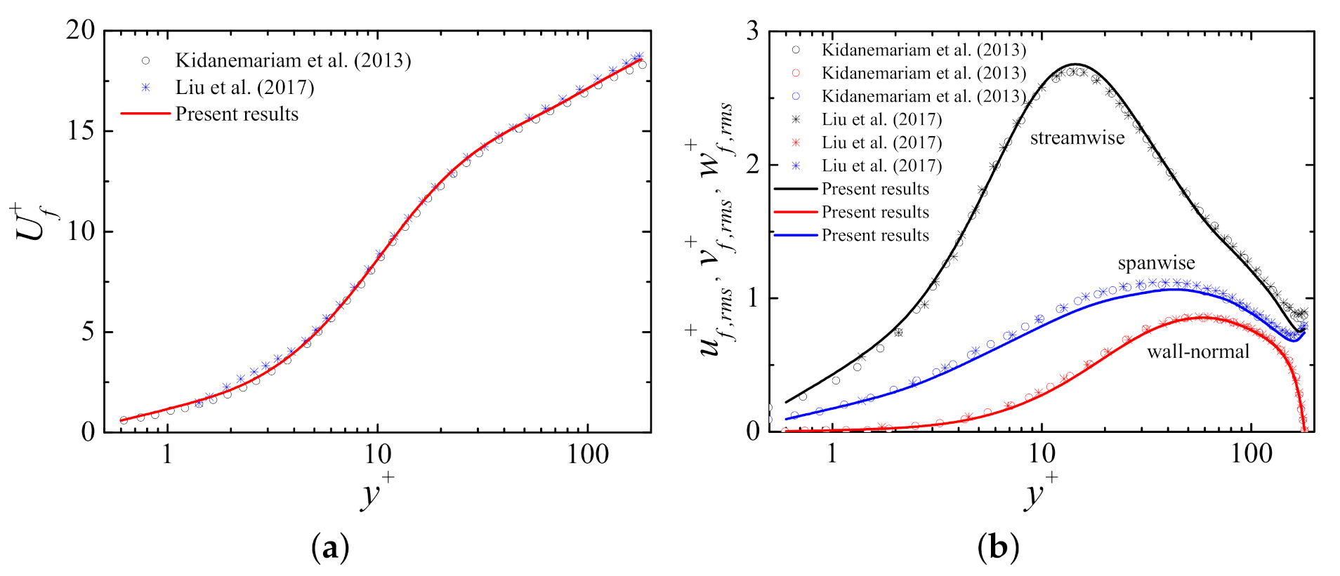
The statistical features of the single-phase flow are validated with the reference data of Kidanemariam et al. [9] and Liu et al. [19]. In the study of Kidanemariam et al. [9], the open channel had a size of $L_x\times L_y\times L_z=12H\times H\times 3H$, and the computational domain was discretized by $3072\times 257\times 768$ grid points. The turbulent flow was solved using a finite difference method based on the N-S equations. In the work of Liu et al. [19], the open channel size was $L_x\times L_y\times L_z=4\pi H\times H\times 2\pi H$, and the computational domain had a grid resolution of $384\times 64\times 384$. The turbulent flow was solved by the finite volume method based on the N-S equations.

Figure 2a shows the comparison results of the fluid mean streamwise velocity profiles. It can be seen that the present method predicts the mean streamwise velocity very well. In Figure 2b, the fluid root-mean-square (RMS) velocity fluctuation components are compared. For each component, a general good agreement is found along the whole channel height. However, slight deviations can be captured, in particular concerning the streamwise velocity fluctuation. This is perhaps due to the domain size in the streamwise direction not being long enough. Peng [13] argued that the streamwise velocity fluctuation was more related to the large-scale flow structures, which requires the size of the computational domain to be large enough, hence the contamination from the periodic boundary condition can be avoided.

Overall, reasonable agreements between the present results and the reference data are achieved, which provide evidences for the acceptable accuracy of the developed LBM codes. From now on, the sediment-turbulence interactions will be investigated in detailed in the following sections.

4. Results and Discussion

4.1. Fluid Statistics

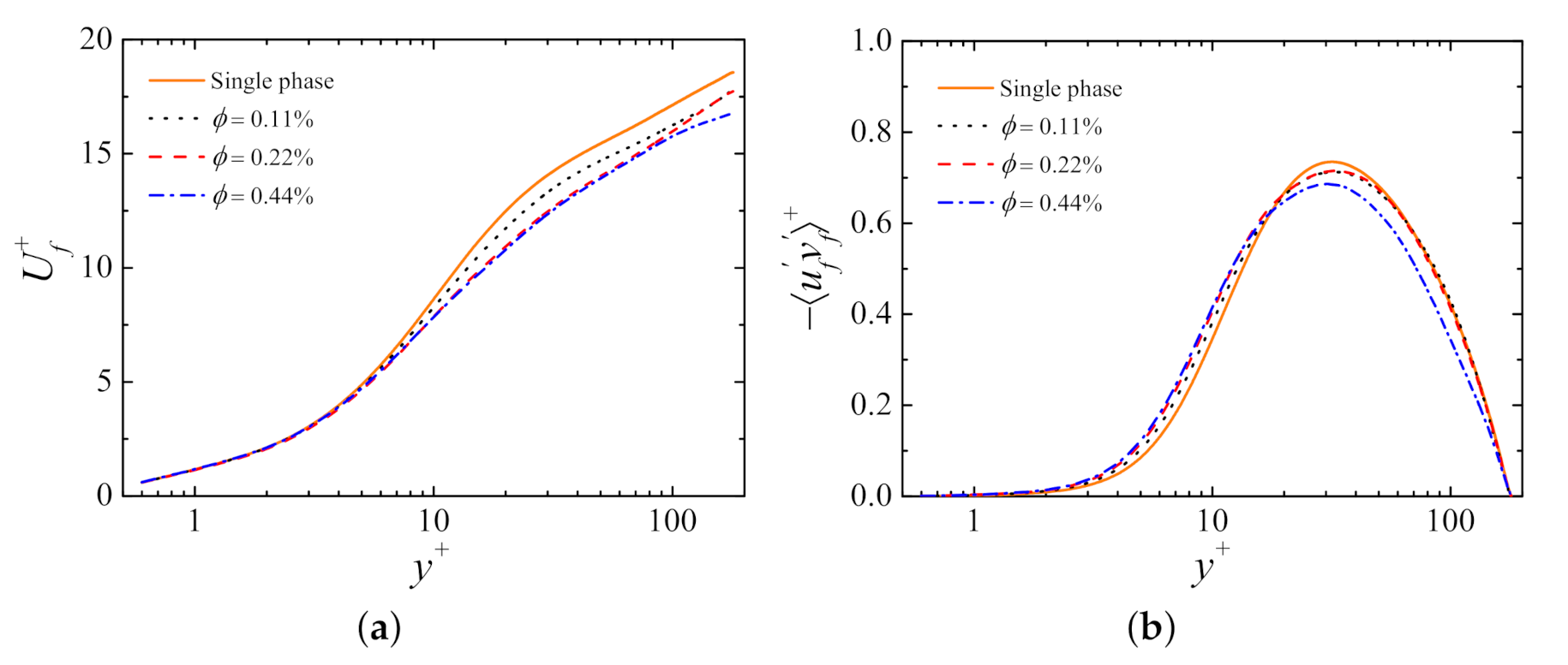
Figure 3a shows the fluid mean streamwise velocity profiles from different cases. It is clearly observed that the streamwise velocity is reduced by the presence of particles, which is consistent with the results reported in particle-laden turbulent pipe flows [15] and channel flows [16] with similar settings. Compared to the single-phase flow, domain-averaged velocity reductions of 5.02%, 7.11%, and 9.22% for cases $\varphi =0.11\%$, 0.22%, and 0.44% are found, respectively. Hence, the velocity reduction is more pronounced at a higher particle volume fraction. It is also seen that all particle-laden cases make the transition from the viscous sublayer to the logarithmic region more gradual. In the logarithmic region ($U_f^{+}=(1/\kappa )ln{y}^{+}+B)$, the von Kármán constant $\kappa$ and additive coefficient B are fitted ($\kappa$, B) = (0.4, 5.72) for the single-phase flow, and ($\kappa$, B) = (0.42, 5.37), (0.34, 2.51), and (0.42, 4.59) for cases $\varphi =0.11\%$, 0.22%, and 0.44%, respectively.

According to the stress balance in a particle-laden channel flow system [13], the fluid mean velocity changes in the sediment-laden cases from their single-phase flow counterpart are related to the change of the Reynolds stress. The Reynolds stress profiles of the four cases are compared in Figure 3b. With respect to the single-phase flow, the Reynolds stresses of the particle-laden simulations are increased in the near-wall region ($y^{+}\le 17$), but decreased in the intermediate region ($17<y^{+}\le 60$), and remain unchanged very close to the top boundary ($175\le y^{+}\le 180$). Peng and Wang [15] pointed out that particles have two opposite influences on the Reynolds stress. On the one hand, particles can filter out the small-scale flow fluctuations due to their finite size. This leads to a reduction in the Reynolds stress. On the other hand, particle rotation in the spanwise direction can produce additional sweep and ejection events through bringing high-speed fluid from the outer region to the wall, and low-speed fluid from the wall to the outer region. This results in the enhancement of the Reynolds stress. Consequently, the overall modulation on the Reynolds stress depends on the competitive mechanisms between the finite size filtration-induced attenuation and the particle rotation-induced enhancement. In the current particulate flows, enhancement due to the particle rotation overwhelms the attenuation induced by the particle filtration near the wall, therefore the Reynolds stress is augmented. Far from the wall, the enhancement mechanism becomes insufficient to compensate the attenuation mechanism, therefore the Reynolds stress is damped.

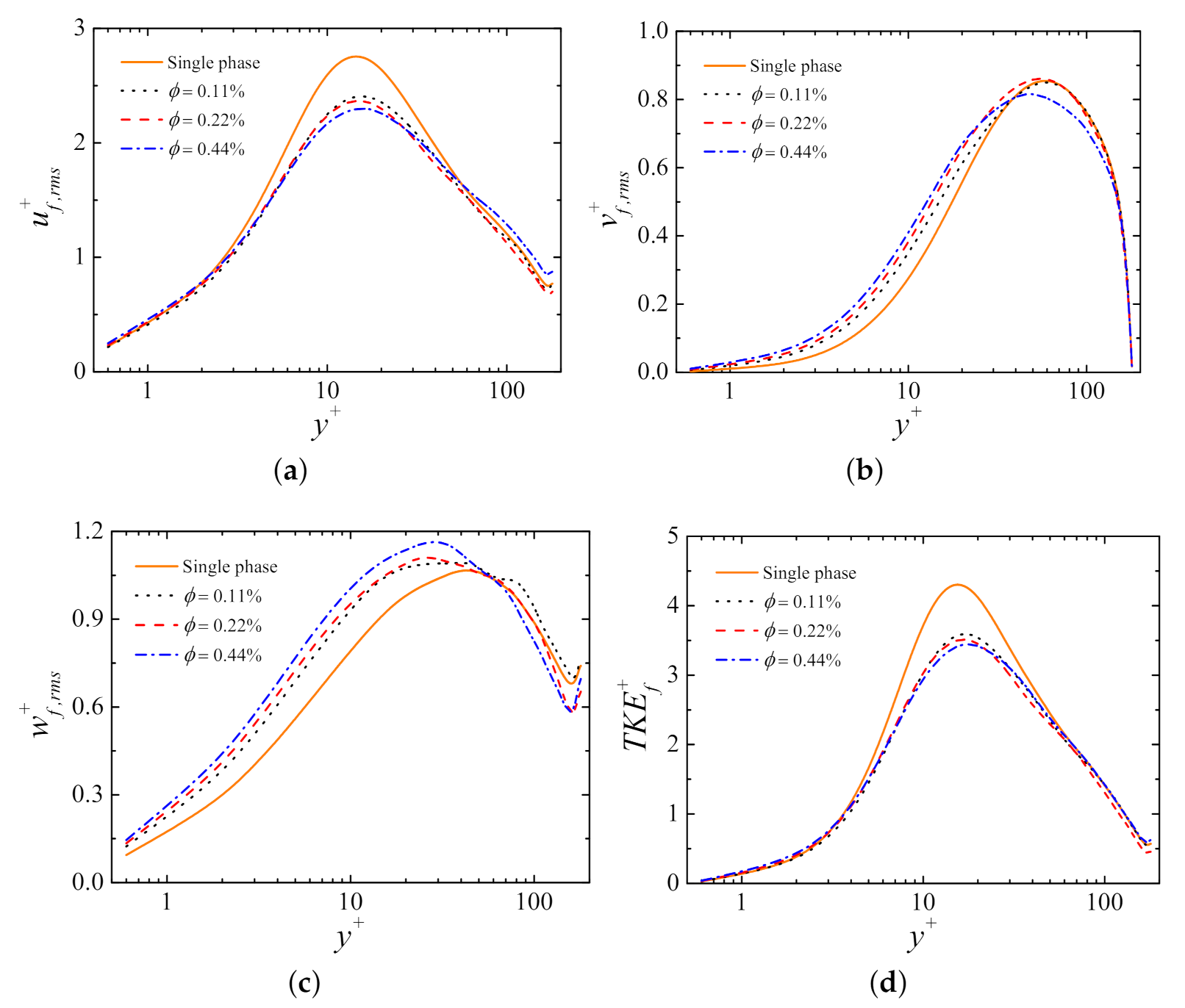
Figure 4a–c show the fluid RMS velocity fluctuation profiles. As seen from Figure 4a, the strength of the streamwise velocity fluctuation is significantly reduced by the particles. Again, a higher volume fraction leads to a stronger reduction. Shao et al. [20] attributed this reduction to the reduced strength of the large-scale streamwise vortices. Close to the wall ($y^{+}\le 30$), the wall-normal and spanwise velocity fluctuations are both increased compared to the unladen case. These increases can be explained by the fact that particles induce many small-scale vortices in the near-wall region (see Figure 5). It is also noted that the three RMS velocity fluctuation profiles become closer to each other in the particle-laden cases with respect to the single-phase flow. This behavior implies that particles make the distribution of the fluid energy towards a more isotropic state among different velocity components, and the modulation increases with the particle volume fraction.

The fluid turbulent kinetic energy (TKE) from different cases are shown in Figure 4d. The fluid TKE is defined as $TK{E}_f^{+}=0.5[{\left(u_{f,rms}^{+}\right)}^2+{\left(v_{f,rms}^{+}\right)}^2+{\left(w_{f,rms}^{+}\right)}^2]$. With the presence of particles, the two-phase flows have lower peak values of TKEs. It indicates that the turbulence activities are generally suppressed by the particles. Overall, the addition of particles is found to result in a more homogeneous TKE distribution in the wall-normal direction, with slightly enhanced TKE in the viscous sublayer and noticeably reduced TKE in the buffer region. Similar behaviors were also found in turbulent channel flows laden with neutrally buoyant particles [13].

4.2. Flow Structures

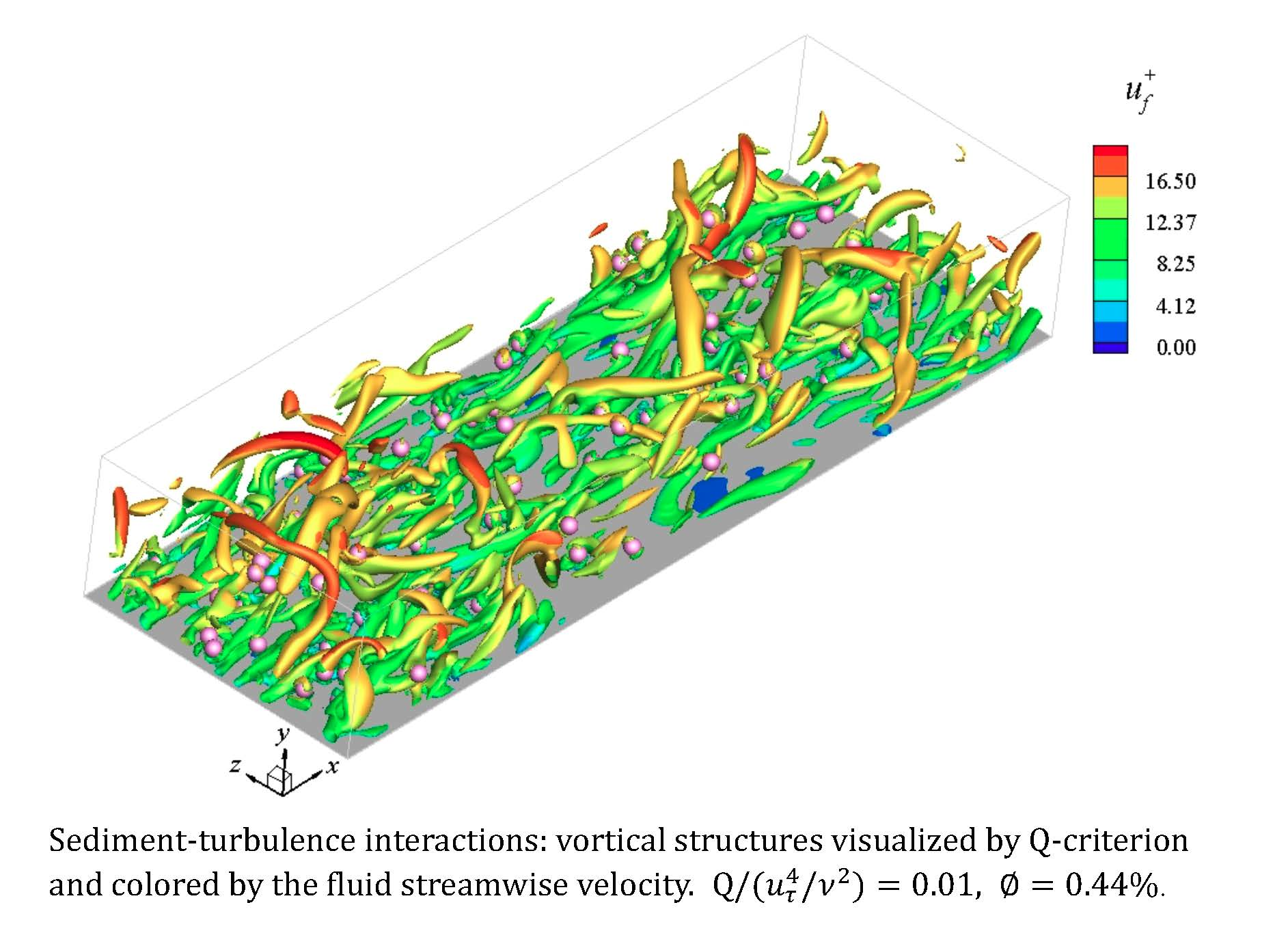
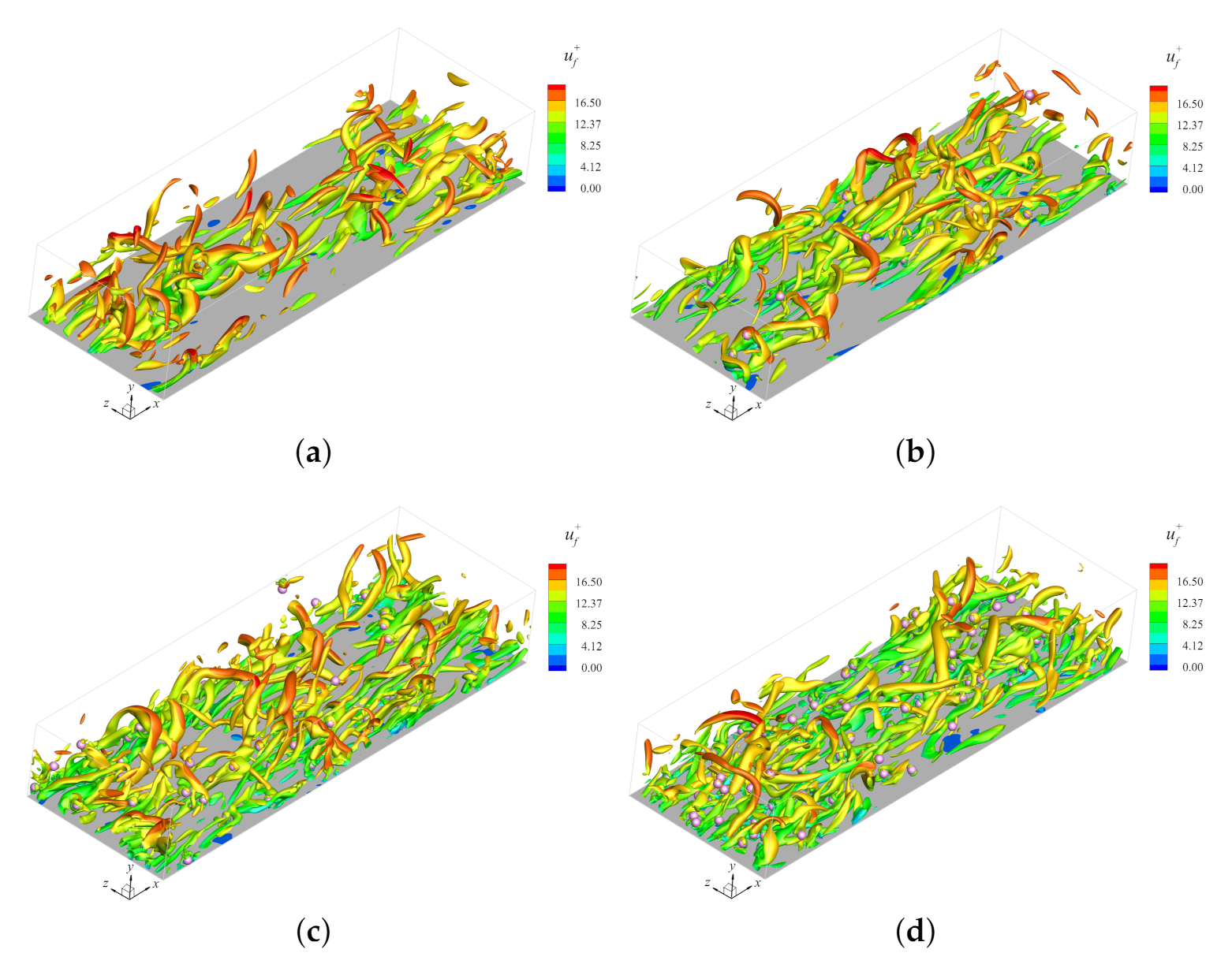
The modulations of the fluid statistics are essentially due to the changes brought by the sediment particles to local flow structures. Figure 5 exhibits the isosurfaces of the second invariant of the velocity gradient tensor, i.e., Q-criterion, which is frequently used to visualize vortical structures in the turbulent flow [30]. The Q-criterion is defined using Einstein summation convention as $Q=(1/4)({\omega }_i{\omega }_i-2S_{ij}{S}_{ij})$, where ${\omega }_i={\epsilon }_{ijk}{\partial }_j{u}_k$ is the vorticity, $S_{ij}=(\partial u_i/\partial x_j+\partial u_j/\partial x_i)/2$ is the strain rate of the velocity fluctuations, and ${\epsilon }_{ijk}$ is the Levi–Civita symbol. In all cases, the large-scale hairpin vortices can be identified, but their occurrence is decreased with the increase of particle volume fraction. With the presence of particles, the suppression of the vortical structures is responsible for the reduction of the maximum value of the fluid streamwise velocity fluctuations [20], as shown in Figure 4a. Compared to the single-phase flow, the particle-laden cases show a considerable amount of small-scale vortices in the near-wall region. The number of these vortices increases monotonically with the particle volume fraction. This is because the particle-turbulence interactions are more intense at a higher particle volume fraction, which lead to more large-scale vortices breaking into small-scale ones. In the numerical work of Eshghinejadfard et al. [21], they pointed out that such small-scale vortices were stronger and more energetic in the particle-laden cases than those in the single-phase flow. These small-scale vortices are the main reason for the enhancements of the fluid wall-normal and spanwise velocity fluctuations in the proximity of the wall, as depicted in Figure 4b,c.

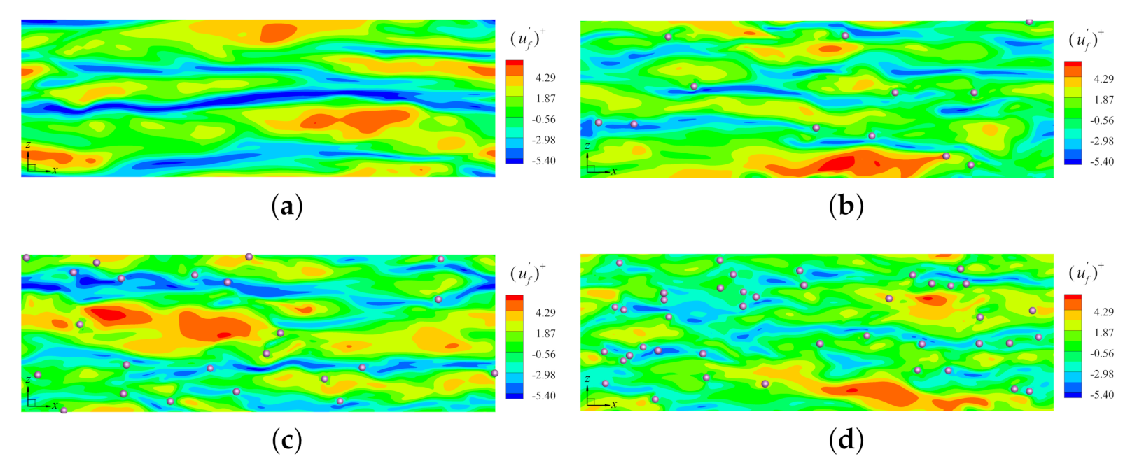
The streamwise vortices exchange the fluid momentum between the inner wall and the outer channel, which creates the well-known high- and low-speed velocity streaks [31]. As the streamwise vortices have been modified by the presence of sediment particles, the velocity streaks structures near the bottom channel wall could also be modulated. To explore this effect, snapshots of the streaky structures at $y^{+}=13.8$ plane are plotted in Figure 6. The reason for choosing this location is because it corresponds to the position with the maximum particle concentration, as depicted in Figure 7a. As shown, the presence of particles breaks the slender low-speed streaks into many smaller ones. Interestingly, the velocity streaks can still be recognized at the highest volume fraction $\varphi =0.44\%$. It is also observed that particles have a tendency to reside in the low-speed streaks. This phenomenon can be explained by the fact that the streamwise vortices tend to drive particles into the low-speed velocity regions. The above observation is in agreement with the simulation results of Kidanemariam et al. [9] ($D/H=0.04$, $\varphi =0.05\%$, ${\rho }_p/{\rho }_f=1.7$, and $\Theta =0.19$) and Shao et al. [20] ($D/H=0.05$ and 0.1, $\varphi$ ranges from 0.79% to 7.08%, ${\rho }_p/{\rho }_f=1.5$, and $\Theta =0.11$ and 0.22) for heavy finite-size particles.

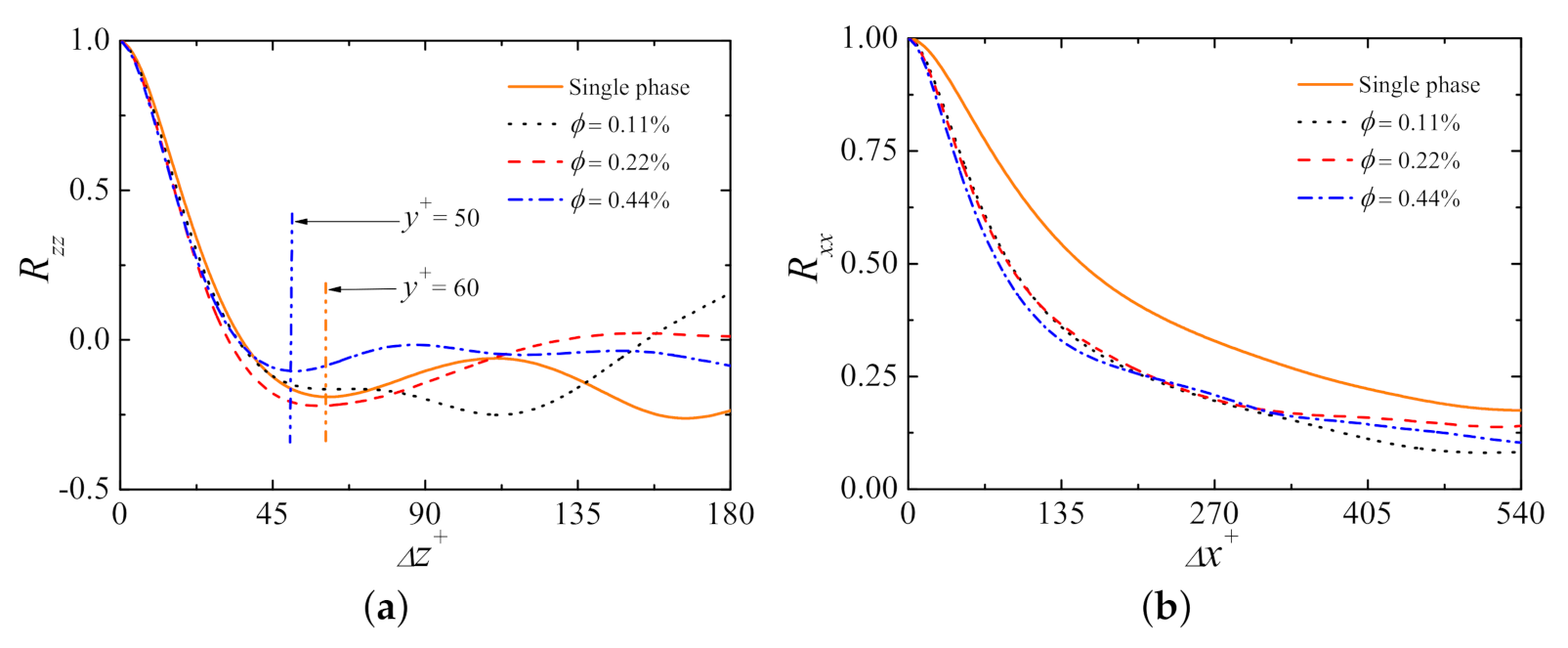
In order to quantitatively evaluate the effect of particles on the streaky structures, the two-point autocorrelation functions at $y^{+}=13.8$ plane are examined. Figure 8 illustrates the autocorrelations of velocity fluctuation components as a function of the spanwise and streamwise separations. The spanwise autocorrelation coefficient is calculated as $R_{zz}(\Delta z)=\overline{u^{{}^{\prime }}(x,y,z)u^{{}^{\prime }}(x,y,z+\Delta z)}/\overline{u^{{}^{\prime }}(x,y,z)u^{{}^{\prime }}(x,y,z)}$, where $\Delta z$ is the spanwise separation and $u^{{}^{\prime }}(x,y,z)$ is the instantaneous streamwise velocity fluctuation. The streamwise autocorrelation coefficient is computed as $R_{xx}(\Delta x)=\overline{u^{{}^{\prime }}(x,y,z)u^{{}^{\prime }}(x+\Delta x,y,z)}/\overline{u^{{}^{\prime }}(x,y,z)u^{{}^{\prime }}(x,y,z)}$, where $\Delta x$ is the streamwise separation. As stated by Kim et al. [33], the streak spacing is roughly twice the spanwise location of the minimum point of $R_{zz}$. It is found in Figure 8a that the streak spacing decreases from $\Delta z^{+}\approx 120$ in the single-phase flow to $\Delta z^{+}\approx 100$ for a volume fraction of $\varphi =0.44\%$. This result confirms the qualitative comparisons between Figure 6a,d. As observed from Figure 8b, the values of $R_{xx}$ are substantially decreased by the existence of particles, which verifies the observations in Figure 6 that particles alters the near-wall turbulent structures to a less organized state.

4.3. Particle Statistics

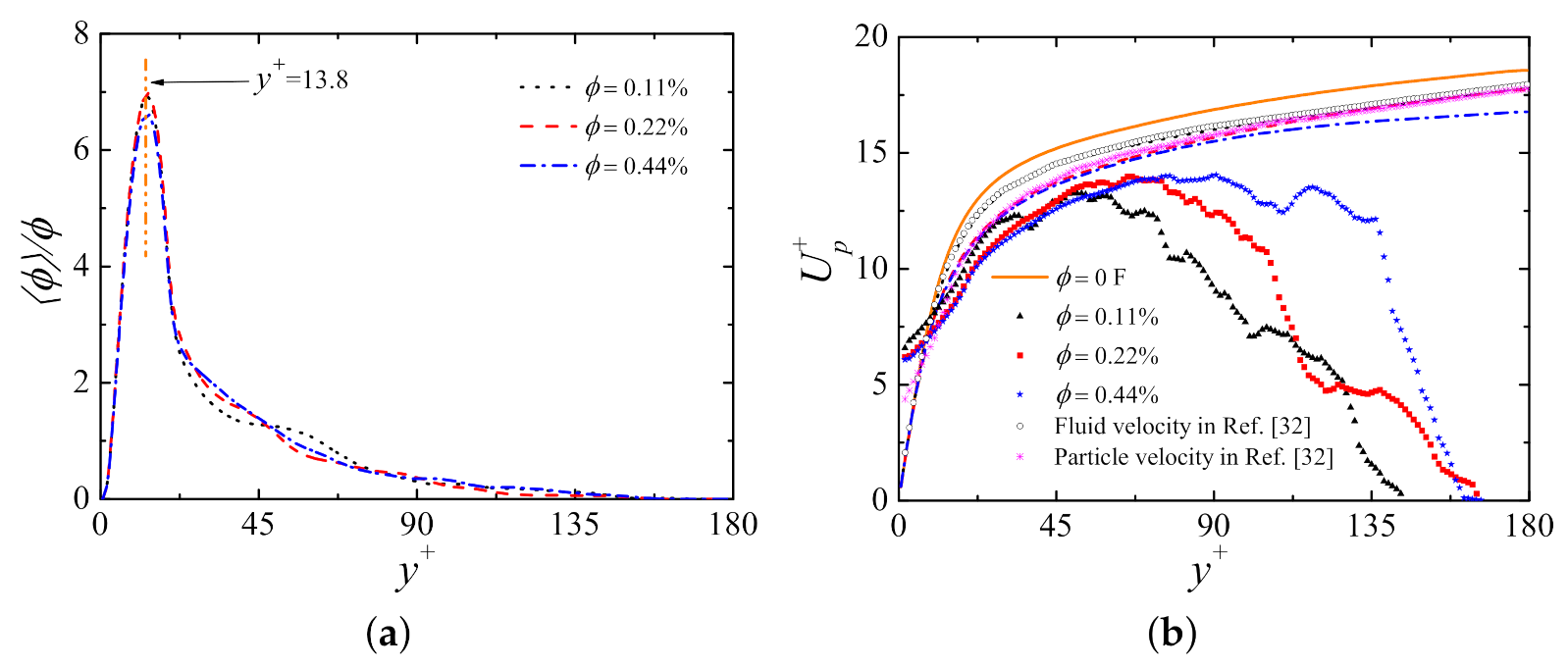
In Figure 7a, the distributions of particle local volume fraction as function of the wall-normal locations are presented. All three profiles show a local maximum point near the wall ($y^{+}=13.8$), followed by a rapid decrease, reaching zero near the upper boundary. Note that, if a particle rests on the wall, its center will be at $y^{+}=9$. Thus the peak position is a dynamic balance between gravity, lubrication force, and turbulent transport. The observed phenomenon is consistent with the experimental measurement by Ni et al. [34] for the sediment particles. Due to the settling effect, most particles locate near the bottom wall (see Figure 9 as an example), leading to a noticeably higher concentration close to the wall. It is also found that all particle-laden curves are self-similar, exhibiting only slight discrepancies across the whole channel. This is because the particle volume fractions are small in all particle-laden cases. Based on the current parameter settings, it might be concluded that the total particle volume fraction has little effect on the normalized concentration profile.

Figure 7b shows the particle mean streamwise velocity profiles together with their fluid counterparts for comparison. At a close proximity to the wall, particles move significantly faster than the fluid phase. This is because the particles can slip on the bottom wall whereas the fluid velocity is constrained by the no-slip condition. A similar observation is also found in the experimental results of Ebrahimian et al. [32] for particle-laden turbulent channel flows (see Figure 7a in their paper, $R{e}_{\tau }=410$, $D^{+}=6.8$, $\varphi =0.03\%$, ${\rho }_p/{\rho }_f=2.65$, and $\Theta =1.49$). As shown ($y^{+}<9$), the mean slip velocity $\Delta U_{pf}^{+}=U_p^{+}-U_f^{+}$ in the present simulation is larger than that in Ref. [32]. Specifically, as $y^{+}\to 0$, $\Delta U_{pf}^{+}$ in case $\varphi =0.44\%$ is approximately 5.81, compared to 3.78 of Ref. [32]. The differences in $\Delta U_{pf}^{+}$ between these two studies perhaps come from the different values of the particle size, friction Reynolds number $R{e}_{\tau }$, and Shields number $\Theta$. In the outer channel, the fluid velocity is obviously larger than the particle velocity. It can be explained by the fact that the solid particles are lifted off by ejection events, perhaps only momentarily, and then settle back down, resulting in a much smaller mean velocity in the outer region relative to the fluid velocity. It is also noted that the particle-laden curves have strong fluctuations in the outer region. The reason is that most particles settle to the near-wall region, the statistical samples are insufficient in the upper section.

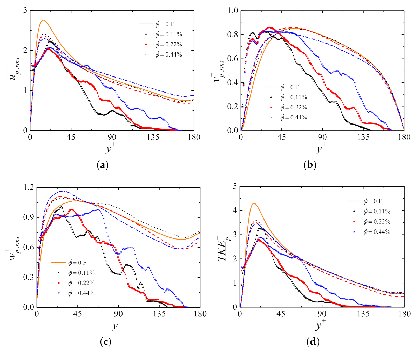
The particle and fluid RMS velocity fluctuations are compared in Figure 10a–c. The particle RMS velocity fluctuations are generally much smaller than those of the fluid phase at the same wall-normal location except for the near-wall region. This is due to the particle inertial effect, preventing fast changes in velocity. In the neighborhood of the wall, it is interesting to find that the particle wall-normal velocity fluctuations are significantly larger than the corresponding fluid components. Similar phenomenon can be also found in the study of Chan-Braun et al. [35] for Shields number $\Theta =0.22$. In Figure 10d, the particle and fluid turbulent kinetic energy (TKE) profiles are compared. The definition of the particle TKE is an analogy to that of the fluid TKE, i.e., $TK{E}_P^{+}=0.5[{\left(u_{p,rms}^{+}\right)}^2+{\left(v_{p,rms}^{+}\right)}^2+{\left(w_{p,rms}^{+}\right)}^2]$. Besides a small region attached to the wall, the particle TKE is lower than that of the fluid phase, which is again due to the particle inertia.

4.4. Particle Dynamics

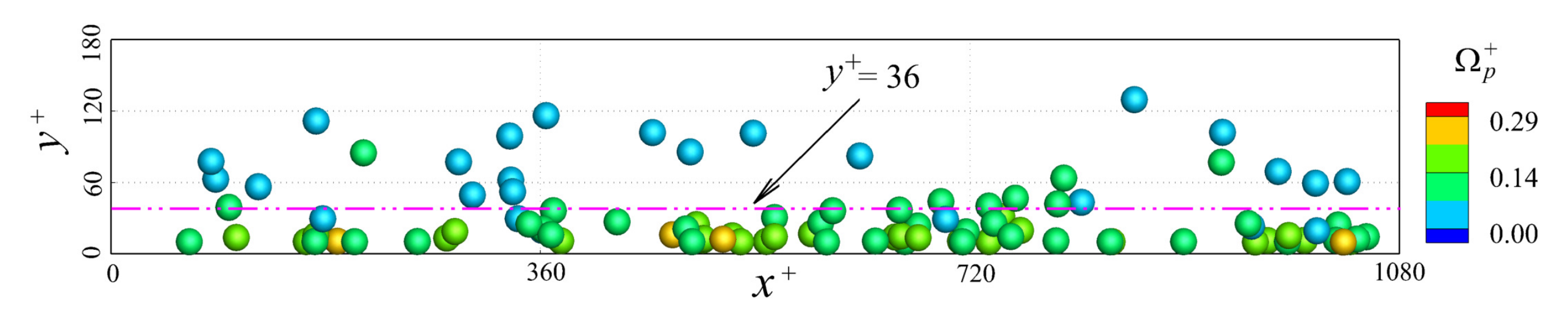
Figure 9 shows the side view snapshot of particle positions from case $\varphi =0.44\%$. As observed, a large number of particles accumulate near the bottom wall whereas a few particles are suspended in the upper channel. This observation is consistent with the particle concentration profiles, as shown in Figure 7a. More specifically, approximately 70% of the particles with their normalized center positions locate in the region $y^{+}\le 36$ (twice the normalized diameter of the particles). In addition, the near-wall particles have obviously larger angular velocities than those in the outer area. One of the main reasons is because the shear stress is decreased with the wall-normal distance. Several typical transport modes of the sediment particles, such as resuspension, saltation, and rolling are captured in the side view animation (see Video S1 in the supplementary materials). It is worth mentioning that resuspension represents the sediment particles being lifted up from the bed and exhibit large jumps to eventually become suspended for a relatively long time; saltation denotes the sediments lose contact with the bed for a short while and their jump heights are within twice the particle diameter; rolling indicates the particles have angular velocities and their movements generally in contact with the bed [18].

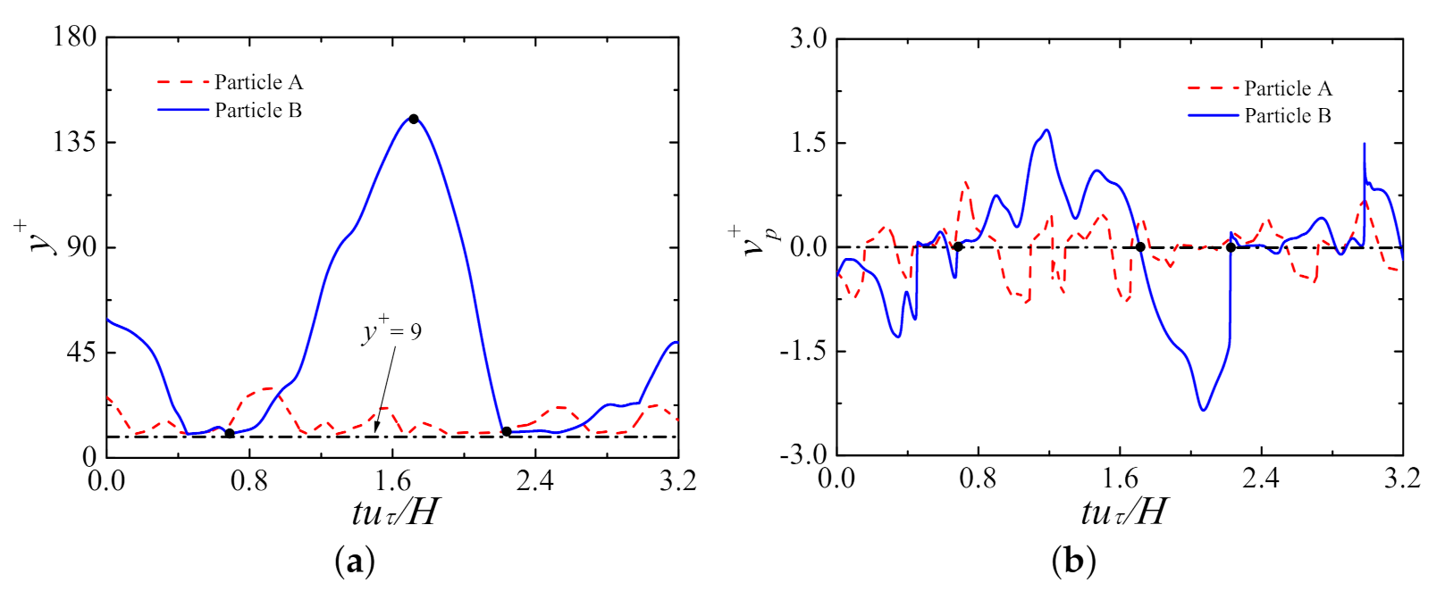
To gain further insight into the particle motions, the wall-normal trajectories of all particles in case $\varphi =0.44\%$ are analyzed for period $0\le t{u}_{\tau }/H\le 3.2$. It should be noted that $t{u}_{\tau }/H=0$ indicates a time when the two-phase flow has reached the statistically steady state. Among them, two typical types of particle trajectories (A and B) are found, as shown in Figure 11a. As observed from Figure 11a, particle A spends all its time residing in the near-wall region and some obvious hops are identified. It could be imagined that the particle-wall collisions are frequent. Moreover, side view animation (see Video S2 in the supplementary materials) visually shows that the major transport modes of this particle are saltation and rolling. It is noted that particle A remains in the lower part of the logarithmic layer and below. The saltation period is roughly $0.5H/u_{\tau }$. It never gains enough energy to enter the outer region.

On the contrary, particle B is occasionally lifted up and entrained by the turbulent eddies so that it resuspends and moves upward to the outer channel and then returns to the bottom wall ($0.7\le t{u}_{\tau }/H\le 2.2$). Its trajectory exhibits evident rising and falling, looking like a ballistic curve. This interesting phenomenon is closely related to the combined effects of turbulent dynamics and gravitational force. The whole process of resuspension and redeposition takes more than one large eddy turnover time.

As for the wall-normal velocities (Figure 11b), particle A experiences more frequent velocity variations (negative-positive-negative) than particle B. This is because particle A almost moves near the bottom wall where the particle-wall and particle-particle interactions are intensive, while particle B is sometimes entrained to the outer region where the particle-turbulence interactions are relatively weak. On the other hand, the velocity fluctuation amplitudes of particle A are overall lower than those of particle B. At $t{u}_{\tau }/H=0.7$, the wall-normal velocity of particle B alters from negative to positive, which means it begins to take off. This moment also indicates the particle reaches the lowest position. Later on, particle B continuously climbs up together with positive vertical velocity until the maximum wall-normal position is reached ($t{u}_{\tau }/H=1.7$). At the early stage of this climbing, the combined effects of the upward forces (i.e., shear-induced lift force and rotation-induced lift force) overwhelm the downward gravitational force and drag force, thereby the particle rapidly accelerates and incessantly rise up. However, at the late stage, the gravitational force and drag force predominate the lift force, hence the particle decelerates till it arrives the peak point. After that, the vertical velocity changes from positive to negative and the particle quickly falls down under the effects of gravity and sweep events. When particle B settles close to the bottom wall, its vertical velocity again decelerates until a particle-wall collision takes place ($t{u}_{\tau }/H=2.2$). This slow down process is owing to the fact that the particle encounters resistances from the turbulence and the bottom wall. The aforementioned transport processes ($0.7\le t{u}_{\tau }/H\le 2.2$), i.e., resuspension and re-sedimentation, could be viewed as a free-flight stage where only the hydrodynamic force and the gravitational force affect the particle motion.

4.5. Particle Clustering

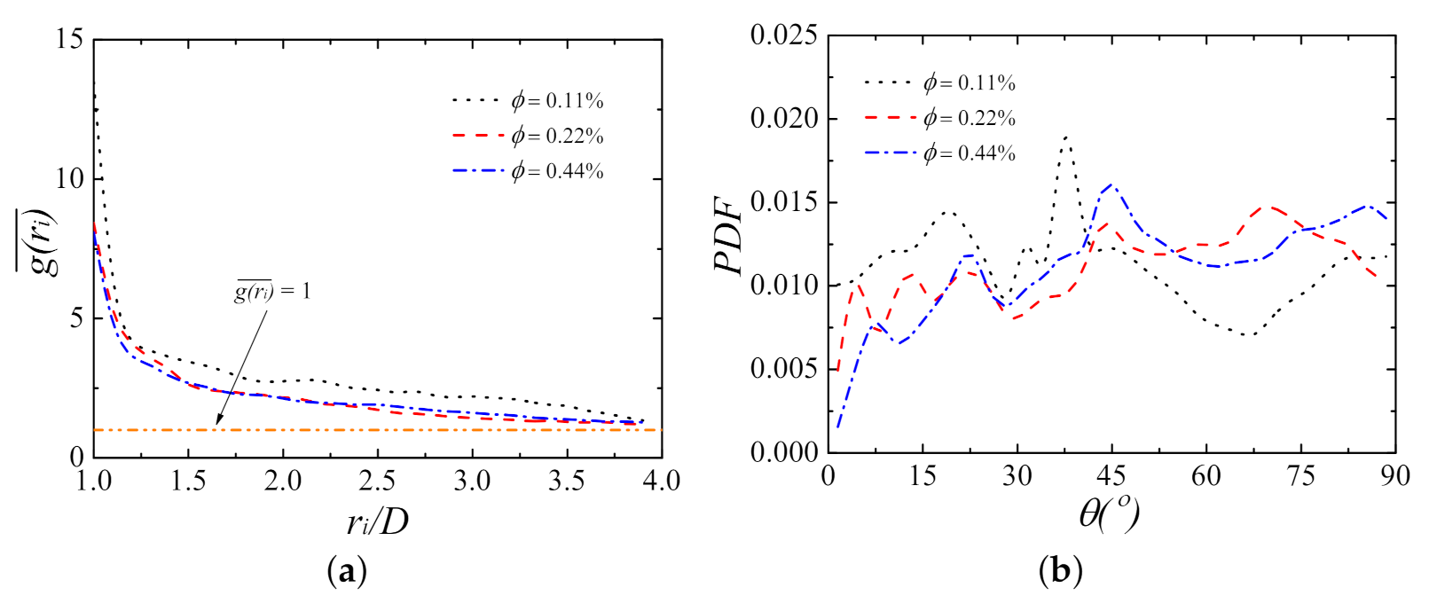
Figure 12a shows the results of the particle radial distribution functions (RDFs), $\overline{g\left(r_i\right)}$. This quantity estimates the probability of finding a second particle at distance $r_i$ away from the target particle, which is defined as $\overline{g\left(r_i\right)}=(N_i/V_i)/(N/V)$, where $r_i$ is the distance of two particle centers, $N_i$ is the number of particle pairs separeted with a distance ($r_i-\Delta r$, $r_i+\Delta r$), $\Delta r$ is set to be $0.1R$ in this simulation; $V_i=4\pi [{(r_i+\Delta r)}^3-{(r_i-\Delta r)}^3]/3$ is the shell volume, $N=N_p(N_p-1)/2$ is the total number of particle pairs in the flow system, and $V=L_x\times L_y\times L_z$ is the total volume of the computational domain. The value of $\overline{g\left(r_i\right)}$ at the distance equals to the particle diameter indicates the level of two-particle clustering. As shown, all particle-laden cases display obvious peaks at the separation distance $r_i=D$, followed by a quick drop, then gradually decrease when $r_i$ further increases. The findings concerning two-particle clustering have the highest RDFs are in line with the simulation results of Lashgari et al. [36], where turbulent channel flows laden with finite-size neutrally buoyant particles were studied.

The probability density functions (PDFs) of the two-particle clustering orientation angles $\theta$ are plotted in Figure 12b. The orientatin angle is defined as $\theta =ta{n}^{-1}(\sqrt{{(y_A-y_B)}^2-{(z_A-z_B)}^2}$/ $\parallel x_A-x_B\parallel )$, where ($x_A$, $y_A$, $z_A$) and ($x_B$, $y_B$, $z_B$) are the center coordinates of two contact partilces A and B, respectively. When $0\le \theta \le {45}^{°}$, the particle clustering aligns towards the streamwise direction; when $\theta >{45}^{°}$, it aligns along the cross-streamwise directions. It is observed that the two-particle clustering seems to uniformly orientate in all angles with the exceptions of the angles around 0 and ${45}^{°}$. Near zero degree, the orientation angles have the lowest probability. This is likely due to the strong particle-turbulence interactions so as to destroy the contact particles exactly align the streamwise direction. It is also interesting to note that the two-particle clustering has a slight preference to orientate close to ${45}^{°}$. The possible reason is closely related to the streamwise vortices who grow outward from the near-wall region with their heads inclining at ${45}^{°}$ to the streamwise direction [37].

4.6. Discussion on the Particle Concentration Distribution

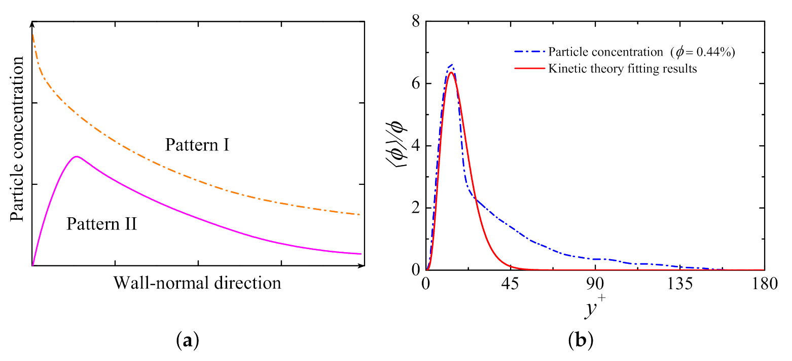
As reported by Wang and Ni [38], there are two different kinds of patterns for the particle concentration distribution in open channels, i.e., pattern I and pattern II, as shown in Figure 13a. Pattern I displays an increasing concentration downward, with a maximum value at the bottom wall. On the other hand, pattern II exhibits the maximum concentration at some position above the bottom wall and then shows the decreasing value towards the wall. The mechanisms for the formations of these two different patterns are primarily ascribed to the lift forces acting on the particles by the surrounding fluid and the wall lubrication force [38]. In general, small heavy particles (${\rho }_p/{\rho }_f>1$) are usually formed the pattern I and it can be modeled by the Rouse formula [39]; while large light particles (${\rho }_p/{\rho }_f\le 1$) commonly form pattern II and it can be modeled by the kinetic theory of particle-fluid two-phase flows, which is given as Equation (12) [38]. Evidently, our current particle concentration distributions belong to the pattern II regime.

$$\frac{C}{C_a}={\left(\frac{\eta }{{\eta }_a}\right)}^{\zeta -1}{e}^{-Z_{*}(\eta -{\eta }_a)},$$

(12)

where C is the vertical concentration at some position y above the bottom, $\eta =y/H$, $C_a$ is a reference concentration at a reference location ${\eta }_a$ (i.e., bed-layer thickness, ${\eta }_a=y_a/H$), and $Z_{*}$ and $\zeta$ denotes the relative dynamic effects of fluid turbulent intensity and particle weight as well as the static characteristics of the fluid and particles in a given sized space. Usually, $Z_{*}$ is a linear function of ${\omega }_s/u_{\tau }$, (i.e., $Z_{*}=a({\omega }_s/u_{\tau }))$, where ${\omega }_s$ is the particle terminal settling velocity; $\zeta$ is related to the particle-fluid density ratio and the particle relative size, (i.e., $\zeta =1+b(D/H)/\sqrt{{\rho }_p/{\rho }_f})$. a and b are two adjustable constants.

In the current fitting, the concentration profile of case $\varphi =0.44\%$ is chosen. The reference location ${\eta }_a$ is set to be 0.01 [40] since no apparent bed-layers are formed, which leads to $C_a=0.12$. Based on Equation (12), the two adjustable parameters a and b are fitted as 23.35 and 56.68, respectively. Figure 13b shows the fitting results versus the actual concentration distribution from case $\varphi =0.44\%$. It is clearly observed that the fitting data and the present concentration match well in the near-wall region, while some differences are detected far away from the wall. Overall, the fitting is reasonable with the R-squared value being 0.85. The deviations might come from two reasons: (i) The different treatments of the particle collisions. In the theoretical model, the particle inter-collisions and particle-wall collisions are neglected. However, in the present simulation, the lubrication force model and the soft-sphere collision model are considered when particle-particle and particle-wall collisions occur; (ii) the theoretical model is derived under the condition of two-dimensional steady state assumption, whereas the current simulation is a three-dimensional sediment-laden flow. Similar deviations were also found in [38] who compared their prediction results with other authors’ experimental data (see Figure 3 in their paper).

5. Conclusions

In this study, interface-resolved direct numerical simulations based on the lattice Boltzmann method are used to explore the sediment-turbulence interactions in the turbulent open channel flows. The effects of different particle volume fractions on the statistics of the fluid and particle phases, flow structures, and particle dynamics are numerically investigated. According to the simulation results, the following conclusions are drawn:

(i)

The presence of heavy particles substantially reduces the maximum fluid streamwise velocity fluctuations, and this effect is more pronounced at a higher particle volume fraction. In the near-wall region, the fluid wall-normal and spanwise velocity fluctuations are both augmented when compared to the single-phase flow. The particles force the TKE to distribute in a more isotropic manner and also make the TKE more homogeneous in the wall-normal direction.

(ii)

By visualizing the vortical structures, it is found that particles suppress the generation of the large-scale coherent vortices and simultaneously create numerous small-scale vortices in the near-wall region. Particles have a tendency to reside in the low-speed velocity regions and alter the streaky structures to a less organized state.

(iii)

Third itemThe particle TKE is much smaller than the fluid TKE except in the region very close to the wall. Under the current parameter settings, the normalized vertical particle concentration profiles are self-similar. Additionally, a general match between the present concentration profile and a theoretical model is found.

(iv)

Owing to the settling effect, most particles accumulate in the vicinity of the bottom wall, where the particle-wall and particle-particle collisions and the particle-turbulence interactions are strongest. By tracking the particle trajectories, different modes of the sediment transport, such as resuspension, saltation, and rolling, are captured.

References

- Rashidi, M.; Hetsroni, G.; Banerjee, S. Particle-turbulence interaction in a boundary layer. Int. J. Multiph. Flow 1990, 16, 935–949. [Google Scholar] [CrossRef]
- Baker, L.J.; Coletti, F. Experimental study of negatively buoyant finite-size particles in a turbulent boundary layer up to dense regimes. J. Fluid Mech. 2019, 866, 598–629. [Google Scholar] [CrossRef]
- Righetti, M.; Romano, G.P. Particle-fluid interactions in a plane near-wall turbulent flow. J. Fluid Mech. 2004, 505, 93–121. [Google Scholar] [CrossRef]
- Dwivedi, A.; Melville, B.W.; Shamseldin, A.Y.; Guha, T.K. Flow structures and hydrodynamic force during sediment entrainment. Water Resour. Res. 2011, 47, 499–509. [Google Scholar] [CrossRef]
- Balachandar, S.; Eaton, J.K. Turbulent dispersed multiphase flow. Annu. Rev. Fluid Mech. 2010, 42, 111–133. [Google Scholar] [CrossRef]
- Maxey, M. Simulation methods for particulate flows and concentrated suspensions. Annu. Rev. Fluid Mech. 2017, 49, 171–193. [Google Scholar] [CrossRef]
- Tenneti, S.; Subramaniam, S. Particle-resolved direct numerical simulation for gas-solid flow model development. Annu. Rev. Fluid Mech. 2014, 46, 199–230. [Google Scholar] [CrossRef]
- Pan, Y.; Banerjee, S. Numerical investigation of the effects of large particles on wall-turbulence. Phys. Fluids 1997, 9, 3786–3807. [Google Scholar] [CrossRef]
- Kidanemariam, A.G.; Chan-Braun, C.; Doychev, T.; Uhlmann, M. DNS of horizontal open channel flow with finite-size, heavy particles at, low solid volume fraction. New J. Phys. 2013, 15, 025031. [Google Scholar] [CrossRef]
- Ji, C.N.; Munjiza, A.; Avital, E.; Ma, J.; Williams, J.J.R. Direct numerical simulation of sediment entrainment in turbulent channel flow. Phys. Fluids 2013, 25, 056601. [Google Scholar] [CrossRef]
- Yousefi, A.; Costa, P.; Brandt, L. Single sediment dynamics in turbulent flow over a porous bed-insights from interface-resolved simulations. J. Fluid Mech. 2020, 893. [Google Scholar] [CrossRef] [Green Version]
- Derksen, J.J. Simulations of granular bed erosion due to a mildly turbulent shear flow. J. Hydraul. Res. 2015, 53, 622–632. [Google Scholar] [CrossRef]
- Peng, C. Study of turbulence modulation by finite-size solid particles with the lattice Boltzmann method. Ph.D. Thesis, University of Delaware, Newark, DE, USA, 2018. [Google Scholar]
- Gao, H.; Li, H.; Wang, L.-P. Lattice Boltzmann simulation of turbulent flow laden with finite-size particle. Comput. Math. Appl. 2013, 65, 194–210. [Google Scholar] [CrossRef]
- Peng, C.; Wang, L.-P. Direct numerical simulations of turbulent pipe flow laden with finite-size neutrally buoyant particles at low flow Reynolds number. Acta Mech. 2019, 230, 517–539. [Google Scholar] [CrossRef]
- Peng, C.; Ayala, O.M.; Wang, L.-P. Flow modulation by a few fixed spherical particles in a turbulent channel flow. J. Fluid Mech. 2020, 884. [Google Scholar] [CrossRef]
- Tang, G.H.; Tao, W.Q.; He, Y.L. Lattice Boltzmann method for simulating gas flow in microchannels. Int. J. Mod. Phys. C 2004, 15, 335–347. [Google Scholar] [CrossRef] [Green Version]
- Rowiński, P.; Banaszkiewicz, M.; Pempkowiak, J.; Lewandowski, M.; Sarna, M. Hydrodynamics-Hydrodynamic and Sediment Transport Phenomena, 1st ed.; Springer: London, UK, 2014. [Google Scholar]
- Liu, X.; Ji, C.N.; Xu, X.L.; Xu, D.; Williams, J.J.R. Distribution characteristics of inertial sediment particles in the turbulent boundary layer of an open channel flow determined using Voronoï analysis. Int. J. Sediment Res. 2017, 32, 401–409. [Google Scholar] [CrossRef]
- Shao, X.M.; Wu, T.H.; Yu, Z.S. Fully resolved numerical simulation of particle-laden turbulent flow in a horizontal channel at a low Reynolds number. J. Fluid Mech. 2012, 693, 319–344. [Google Scholar] [CrossRef]
- Eshghinejadfard, A.; Zhao, L.H.; Thévenin, D. Lattice Boltzmann simulation of resolved oblate spheroids in wall turbulence. J. Fluid Mech. 2018, 849, 510–540. [Google Scholar] [CrossRef]
- Peng, Y.; Luo, L.S. A comparative study of immersed-boundary and interpolated bounce-back methods in LBE. Prog. Comput. Fluid Dyn. 2008, 8, 156–167. [Google Scholar] [CrossRef] [Green Version]
- Bouzidi, M.; Firdaouss, M.; Lallemand, P. Momentum transfer of a Boltzmann-lattice fluid with boundaries. Phys. Fluids 2001, 13, 3452–3459. [Google Scholar] [CrossRef]
- Zhao, W.F.; Yong, W.A. Single-node second-order boundary schemes for the lattice Boltzmann method. J. Comput. Phys. 2017, 329, 1–15. [Google Scholar] [CrossRef] [Green Version]
- Wen, B.; Zhang, C.Y.; Tu, Y.S.; Wang, C.L.; Fang, H.P. Galilean invariant fluid-solid interfacial dynamics in lattice Boltzmann simulations. J. Comput. Phys. 2014, 266, 161–170. [Google Scholar] [CrossRef] [Green Version]
- Caiazzo, A.; Junk, M. Boundary forces in lattice Boltzmann: Analysis of momentum exchange algorithm. Comput. Math. Appl. 2008, 55, 1415–1423. [Google Scholar] [CrossRef]
- Brändle de Motta, J.C.; Breugem, W.P.; Gazanion, B.; Estivalezes, J.L.; Vincent, S.; Climent, E. Numerical modelling of finite-size particle collisions in a viscous fluid. Phys. Fluids 2013, 25, 083302. [Google Scholar] [CrossRef] [Green Version]
- Breugem, W.P. A combined soft-sphere collision/immersed boundary method for resolved simulations of particulate flows. In Proceedings of the ASME 2010 3rd Joint US-European Fluids Engineering Summer Meeting and 8th International Conference on Nanochannels, Microchannels, and Minichannels, Montreal, QC, Canada, 1–5 August 2010. [Google Scholar]
- Lammers, P.; Beronov, K.N.; Volkert, R.; Brenner, G.; Durst, F. Lattice BGK direct numerical simulation of fully developed turbulence in incompressible plane channel flow. Comput. Fluids 2006, 35, 1137–1153. [Google Scholar] [CrossRef]
- Zhou, J.; Adrian, R.J.; Balachandar, S.; Kendall, T.M. Mechanisms for generating coherent packets of hairpin vortices in channel flow. J. Fluid Mech. 1999, 387, 353–396. [Google Scholar] [CrossRef]
- Blackwelder, R.F.; Eckelmann, H. Streamwise vortices associated with the bursting phenomenon. J. Fluid Mech. 1979, 94, 577–594. [Google Scholar] [CrossRef]
- Ebrahimian, M.; Sanders, R.S.; Ghaemi, S. Dynamics and wall collision of inertial particles in a solid-liquid turbulent channel flow. J. Fluid Mech. 2019, 881, 872–905. [Google Scholar] [CrossRef]
- Kim, J.; Moin, P.; Moser, R. Turbulence statistics in fully developed channel flow at low Reynolds number. J. Fluid Mech. 1987, 177, 133–166. [Google Scholar] [CrossRef] [Green Version]
- Ni, J.R.; Wang, G.Q.; Borthwick, A.G.L. Kinetic theory for particles in dilute and dense solid-liquid flows. J. Hydraul. Eng. 2000, 126, 893–903. [Google Scholar] [CrossRef]
- Chan-Braun, C.; García-Villalba, M.; Uhlmann, M. Direct numerical simulation of sediment transport in turbulent open channel flow. In High Performance Computing in Science and Engineering; Springer: Berlin/Heidelberg, Germany, 2010. [Google Scholar]
- Lashgari, I.; Picano, F.; Costa, P.; Breugem, W.P.; Brandt, L. Turbulent channel flow of a dense binary mixture of rigid particles. J. Fluid Mech. 2017, 818, 623–645. [Google Scholar] [CrossRef] [Green Version]
- Robinson, S.K. Coherent motions in the turbulent boundary layer. Annu. Rev. Fluid Mech. 1991, 23, 601–639. [Google Scholar] [CrossRef]
- Wang, G.Q.; Ni, J.R. Kinetic theory for particle concentration distribution in two phase flow. J. Eng. Mech. 1990, 116, 2738–2748. [Google Scholar] [CrossRef] [Green Version]
- Rouse, H. Modern conceptions of the mechanics of turbulence. Trans. Am. Soc. Civ. Eng. 1937, 102, 463–505. [Google Scholar] [CrossRef]
- van Rijn, L.C. Sediment Transport, Part II: Suspended Load Transport. J. Hydraul. Eng. 1984, 110, 1613–1641. [Google Scholar] [CrossRef]
Figure 1.
Schematic diagram of the open channel laden with finite-size sediment particles.
Figure 2.
Comparison of results between the single-phase flow and the reference data: (a) Fluid mean streamwise velocity and (b) fluid root-mean-square (RMS) velocity fluctuation components.
Figure 3.
Comparison of results between the single-phase flow and the particle-laden flows: (a) Fluid mean streamwise velocity profiles and (b) fluid Reynolds stress profiles.
Figure 4.
(a–c) Fluid RMS velocity fluctuations in the streamwise, wall-normal, and spanwise directions, respectively, and (d) fluid turbulent kinetic energy (TKE).
Figure 5.
Vortical structures visualized by the Q-criterion at and colored by the fluid streamwise velocity: (a) Single phase, (b) , (c) , and (d) .
Figure 6.
Snapshots of the streaky structures at plane: (a) Single phase, (b) , (c) , and (d) . Particles in contact with this plane are also shown.
Figure 7.
(a) Distributions of particle local volume fraction as function of the wall-normal locations and (b) particle mean streamwise velocity profiles. In (b), the corresponding profiles of the fluid phase are also shown for comparison (lines). Besides, mean velocity profiles of the fluid and the particles in Ref. [32] (see Figure 7a in their paper) are also added for comparison.
Figure 8.
Autocorrelation coefficients of the streamwise velocity fluctuations versus the separations at plane: (a) In the spanwise direction and (b) in the streamwise direction.
Figure 9.
Side view snapshot of the particle positions taken from case , particles are colored by their angular velocities. Animations can be found in Video S1 in the supplementary materials.
Figure 10.
(a–c) Intensities of the particle RMS velocity fluctuations in the streamwise, wall-normal, and spanwise directions, respectively, and (d) particle turbulent kinetic energy (TKE). The corresponding profiles of the fluid phase are also shown for comparison (lines).
Figure 11.
Time histories of two typical particle wall-normal motions extracted from case = 0.44%: (a) Center positions and (b) center velocities. If a particle touches the bottom wall, its normalized center position in the wall-normal direction is at . Transport times , 1.7, and 2.2 are marked with symbol “• ”. Side view animation can be found in Video S2 in the Supplementary Materials.
Figure 12.
(a) The radial distribution functions (RDFs) as a function of center-to-center distance and (b) probability density functions (PDFs) of the particle-pair orientation angles.
Figure 13.
(a) Two different patterns of the particle concentration distribution and (b) particle concentration profile from case versus a fitting curve based on the kinetic theory.
Publisher’s Note: MDPI stays neutral with regard to jurisdictional claims in published maps and institutional affiliations. |
© 2021 by the authors. Licensee MDPI, Basel, Switzerland. This article is an open access article distributed under the terms and conditions of the Creative Commons Attribution (CC BY) license (https://creativecommons.org/licenses/by/4.0/).
Share and Cite
MDPI and ACS Style
Hu, L.; Dong, Z.; Peng, C.; Wang, L.-P. Direct Numerical Simulation of Sediment Transport in Turbulent Open Channel Flow Using the Lattice Boltzmann Method. Fluids 2021, 6, 217. https://0-doi-org.brum.beds.ac.uk/10.3390/fluids6060217
AMA Style
Hu L, Dong Z, Peng C, Wang L-P. Direct Numerical Simulation of Sediment Transport in Turbulent Open Channel Flow Using the Lattice Boltzmann Method. Fluids. 2021; 6(6):217. https://0-doi-org.brum.beds.ac.uk/10.3390/fluids6060217
Chicago/Turabian StyleHu, Liangquan, Zhiqiang Dong, Cheng Peng, and Lian-Ping Wang. 2021. "Direct Numerical Simulation of Sediment Transport in Turbulent Open Channel Flow Using the Lattice Boltzmann Method" Fluids 6, no. 6: 217. https://0-doi-org.brum.beds.ac.uk/10.3390/fluids6060217