Evaluation of Turbulent Jet Characteristic Scales Using Joint Statistical Moments and an Adaptive Time-Frequency Analysis

Abstract

This paper presents an analysis of turbulence characteristic scales and eddy convection velocity of jet flows computed using joint statistical moments, digital filters, and a modified version of the empirical mode decomposition (EMD). The ongoing aim of this study is to develop semi-empirical space-time cross-correlation models based on stationary statistics and jet physical lengths. Multivariate statistics are used to correlate jet properties to one-dimensional time series. The data available to this study were recorded from single-point and two-point hot-wire anemometry experiments carried out for a range of jet Mach numbers ($0.2\le M\le 0.8$). Firstly, the jet eddy convection velocity, turbulence length, and time scales are computed using space-time cross-correlation functions. Isotropic flow and frozen turbulence hypothesis are then used to estimate the joint moments from single-point statistics in the fully developed turbulence region. An EMD-based decomposition method is presented and assessed in both the Gaussian and non-Gaussian signal regions. It is demonstrated that the artificially filtered signal reconstructs the physical properties of single and multi-point jet statistics. The relationship between central moments and joint moments presented here focuses on the region of high turbulence levels, which generates the vast majority of jet mixing noise produced by turbofan engines. Further analysis is required to extend this investigation to intermittent zones and other jet noise sources, such as jet-surface installation noise.

1. Introduction

Turbulent jet flows have been studied extensively due to their wide application in engineering systems and their importance in improving our understanding of turbulence. Jets are produced by several propulsion systems used in aviation, playing a major role in propulsion efficiency, as well as aviation gas and noise emissions. Additionally, turbulent jet flows are relatively easily reproducible and controlled in laboratory experiments. For almost one century, unsteady jet properties have been studied extensively to shed light on the physics of self-similar turbulent flows.

The main characteristic lengths of a round jet are the diameter measured at the nozzle exit, the potential core length, the jet spreading angle, and the shear layer width. Early investigations focused on regions several dozen jet diameters downstream of the nozzle exit [1,2,3,4]. In these far-downstream locations, the jet is self-similar, and the properties of simplifying hypothesis can be verified (i.e., homogeneous, isotropic turbulence, and frozen turbulence). However, for modern engineering applications, the turbulence properties in the initial and transitional regions of the jet (i.e., up to ten jet diameters downstream of the nozzle exit), especially at the nozzle exit plane, are essential for noise mitigation and noise prediction [2,5,6]. The industry still relies on relatively simple, semi-empirical methods to predict jet mixing noise and inform the design of novel turbofan engines [7,8,9].

Statistical analysis has been extensively used to define characteristic velocities and characteristic length scales, which define self-similar parameters to the initial region of jets. The classical integral turbulence scales defined from the space-time cross-correlation functions in the frequency and time domains [10,11,12] have been quantified in several works [13,14,15,16]. The vast majority of these experiments have been performed for the stream-wise velocity component, which dominates both the central moments and joint statistics in jets [17,18,19].

The integral scales have been demonstrated to be frequency-dependent [5,20,21]. Hot-wire anemometry is a popular technique for studying turbulence scales due to its high-frequency resolution and low-cost. The development of very small, reliable hot-wire probes prompted several researchers to revisit early experiments on single-point and two-point statistics of jet flows [21,22]. This investigation on incompressible jets was taken further to account for high-subsonic jet speeds under static and in-flight conditions [23,24,25]. Hot-wire measurements are complemented by LES flow-field analyses [17,19,26] and particle image velocimetry [27], in which larger portions of the jet are surveyed.

This paper quantifies the turbulence integral scales and eddy convection velocity in the plume of a round, cold, subsonic jet. The databases presented in [23,25] are explored. In the original research, the focus has been on a limited region of the jet plume. This paper will explore additional jet locations by analysing additional data, applying artificial filtering and empirical mode decomposition (EMD) techniques to separate the contribution of large-scale and small-scale structures on the jet statistics. Furthermore, this paper aims to put the basis on isolating frequency-localized jet features, which should be the input of stochastic models able to predict the jet statistics. In doing so, we aim to identify situations in which only the stationary statistics are necessary to model the characteristic scales in the jet plume, thus avoiding expensive numerical simulations or wind tunnel experiments.

The paper is structured as follows. The next section provides key information about the experimental dataset used, which is presented in the next section. In Section 3, the statistical models used in this work, namely, joint statistics, digital filters, and EMD, are briefly described. Results are presented in Section 4, Section 5 and Section 6, where the jet turbulence time scales, eddy convection velocity, and length scales are computed using the signal decomposition methods.

2. Materials and Methods

The analysis presented in the paper utilizes experimental data acquired in the Doak Laboratory, located at the University of Southampton, UK. These tests were conducted in the original Static Jet Rig (SJR), which is now superseded by a Flight-Jet Rig. Information about the facility equipped with the SJR is provided in the next section.

2.1. Experimental Facility and Hardware

The original static jet rig was active in the Doak Laboratory from the late 2000s to 2017. This rig was mounted in an anechoic chamber with a length of 15 m, a width of 7 m, and a height of 5 m. A compressor-reservoir system supplied air at a maximum pressure of 20 bar. Undesirable flow fluctuations and rig noise were diminished in a labyrinth-type plenum. Two valves were used to obtain the nominal jet velocity at the nozzle exit. A stainless steel convergent nozzle measuring 38 mm in diameter was used in the experiments. The high-speed air exhausted by the nozzle then exited the anechoic chamber via a natural exhaust system.

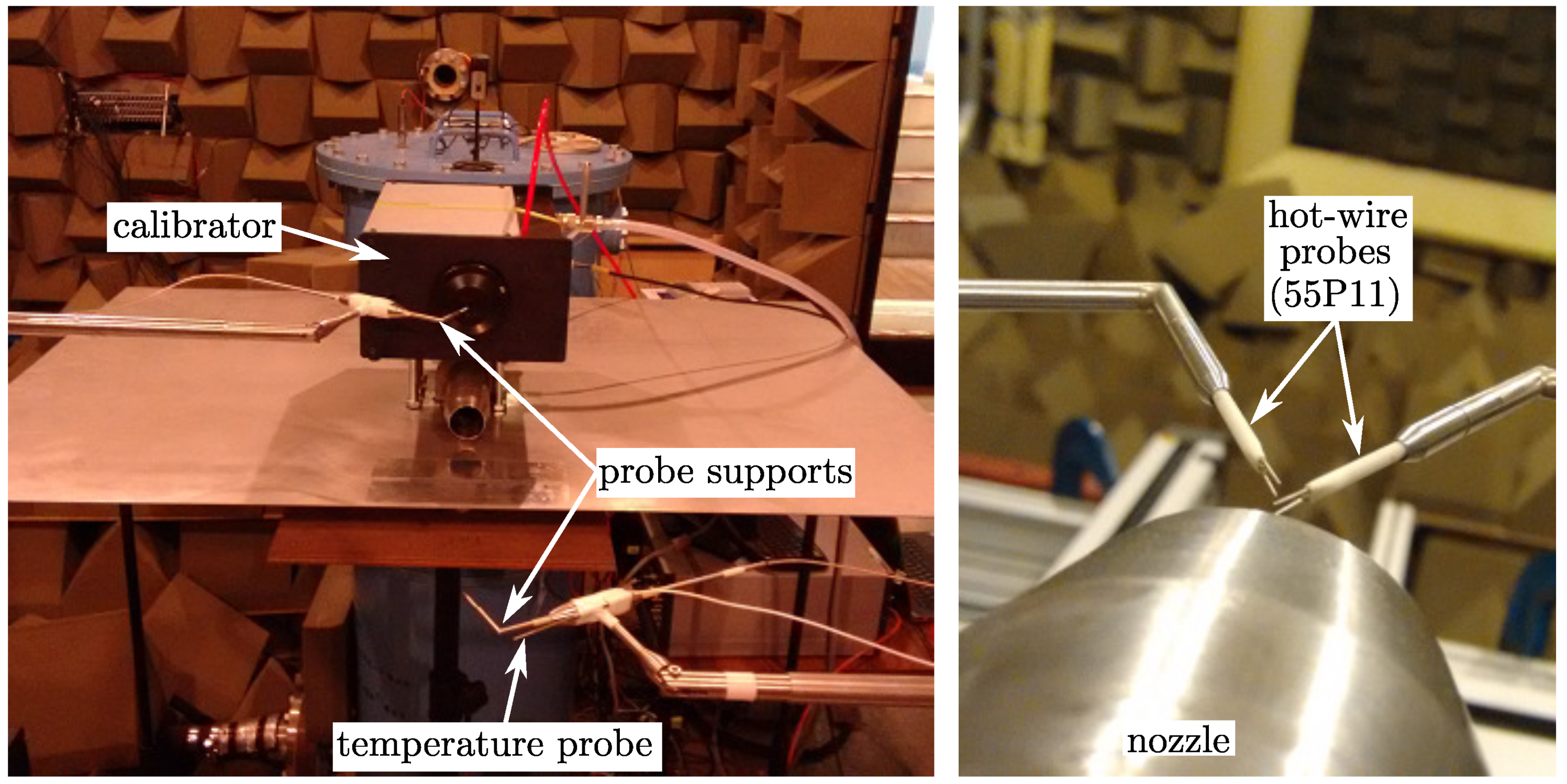
A constant temperature anemometry (CTA) system was used to acquire unsteady velocity data. Single-point and two-point measurements using Dantec 55P01 single hot-wire probes were carried out. These probes were mounted to two ISEL traverse systems, allowing for automatic traverses in three orthogonal axes. Figure 1 illustrates the hot-wire setup and automatic calibrator unit. Note that the installed configuration using the plate displayed in the figure below is beyond the scope of the present work.

Pressure and temperature rakes are located above the plenum (blue chamber in Figure 1) and are used to compute and control the jet nominal velocity. More information about the SJR can be found in [23,25].

2.2. Coordinate System and Jet Properties

The jet studied in this work is nominally axisymmetric. Care was taken to align the two traverse systems with the jet nozzle. The difference between the geometrical jet axis and the measured jet axis was found to be $\pm 0.5^{\circ }$ [16].

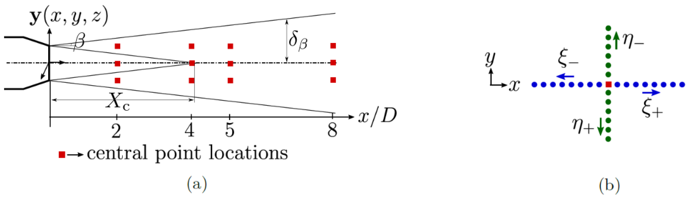
The origin of the jet coordinate system (i.e., $\mathbf{y}(x,y,z)$) is defined at the nozzle exit plane, and at the centre of the nozzle. In two-point tests, the stationary (reference) probe was positioned on four axial locations, along both the centreline and lipline. A separate coordinate system is used for the moving sensor, namely, $\zeta (\xi ,\eta ,\Delta \theta )$. An illustration of the reference probe locations and separation directions initially studied in this paper is displayed in Figure 2. As the final analysis focuses on the stream-wise velocity statistics within the region of high turbulent kinetic energy (i.e., jet lipline), only the separations performed along the axial direction $\zeta (\xi ,0,0)$ are interrogated.

The next section introduces the techniques used to post-process the available experimental data.

3. Joint Moments and Models

As mentioned in the Introduction, jet characteristic scales and convection velocities are studied using different techniques. This section summarises the three tools used in the investigation, namely, cross-correlation coefficients, empirical mode decomposition, and digital filters.

3.1. Cross-Correlation and Coherence Models

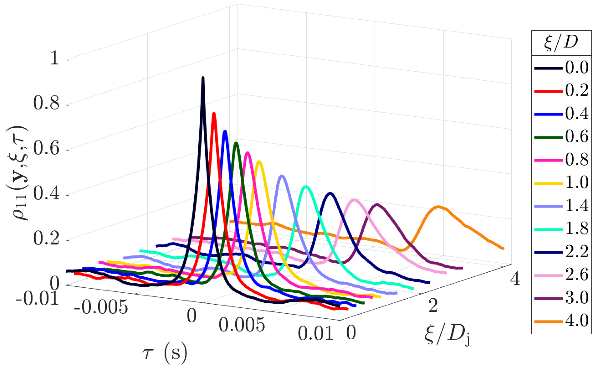
Cross-correlation and coherence functions applied to the experimental data used in this paper were investigated extensively in previous works [16,23]. The general form of the space-time correlation coefficients discussed here is given by,

$${\rho }_{11}\left(\mathbf{y},\zeta ,\tau \right)=\frac{\overline{u^{\prime }\left(\mathbf{y},t\right)u^{\prime }\left(\mathbf{y}+\zeta ,t+\tau \right)}}{\sqrt{\overline{u^{{\prime }^2}}\left(\mathbf{y}\right)\overline{u^{{\prime }^2}}\left(\mathbf{y}+\zeta \right)}},$$

(1)

where the subscripts ‘11’ indicate that only the streamwise velocity component is considered. Autocorrelation coefficients are obtained for $\zeta =0$.

Figure 3 displays an example of the cross-correlation coefficients obtained from the experimental database. The reference sensor is located at $x/D_{\mathrm{j}}=8$ and several separation distances are shown. Both sensors are located on the lipline and, therefore, the separation vector is along the streamwise direction $\xi$.

Length scales and time scale models proposed in a previous work [23] are revisited in this paper. In summary, characteristic scales and eddy convection velocity are self-similar in the high-turbulence intensity region (i.e., along the jet lipline or in the fully developed region several potential core lengths downstream of the jet nozzle exit). The focus of this preliminary study is on this developed region. Self-similarity does not hold true, however, in the nominally laminar potential core region and in the highly intermittent region close to the edge of the jet shear layer.

Time-domain statistics (i.e., space-time cross-correlation and autocorrelation functions) and frequency-domain statistics (i.e., cross-power spectral density and autospectrum) in the jet flow field were previously studied in detail [23]. However, no attempt to correlate the time and frequency-domain models has been pursued. This is conducted here using EMD and digital filters to extract simple statistical trends from the hot-wire signals. The EMD model and digital filters used are discussed in the following sub-sections.

3.2. Empirical Mode Decomposition

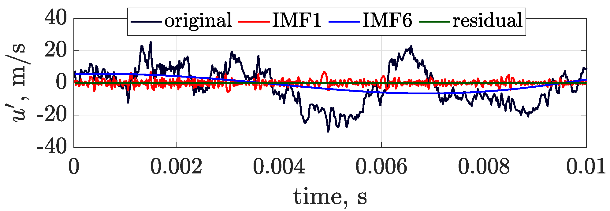
The empirical mode decomposition (EMD) models a signal as a sum of oscillatory components called intrinsic mode functions (IMFs). This method has gained a lot of interest in signal analysis in the past decade, mainly because it is able to separate stationary and non-stationary components from a signal [28]. The EMD is a fully data-driven, unsupervised signal decomposition and does not need any a priori defined basis system [29]. Furthermore, this decomposition method is adaptive and, therefore, highly efficient. The decomposition method is defined by the following Equation [30]:

$$x\left(t\right)=\sum _{k=1}^{K-1}{\mathrm{IMF}}_k\left(t\right)+\mathrm{residual}.$$

(2)

An example of the decomposition applied to a sample set of hot-wire data is displayed in Figure 4. Only the first and sixth IMFs are illustrated. As suggested by the nature of the IMF signals, the first intrinsic modes capture the behaviour of the small-scale structures of the flow, whilst the high IMFs represent the low-frequency behaviour. The several signals obtained by using Equation (2), however, cannot specify a frequency bandwidth between each IMF.

More recently, several modified versions of the EMD have been published in the literature. In one of these works, the cut-off frequency between modes can be selected by using time-varying filters (TVF) [31]. Although this frequency cut-off selection is performed indirectly by setting a bandwidth size, it serves well the purposes of the present work, which is to select a frequency range for large-scale and small-scale structures based on the jet plume single-point statistics. Additionally, the time-varying filter approach is ideal for relatively small time series. This is certainly not a problem for the dataset used here and general hot-wire measurements, but the ability to cope with small, non-stationary time series constitutes a great advantage for other experimental techniques and numerical methods.

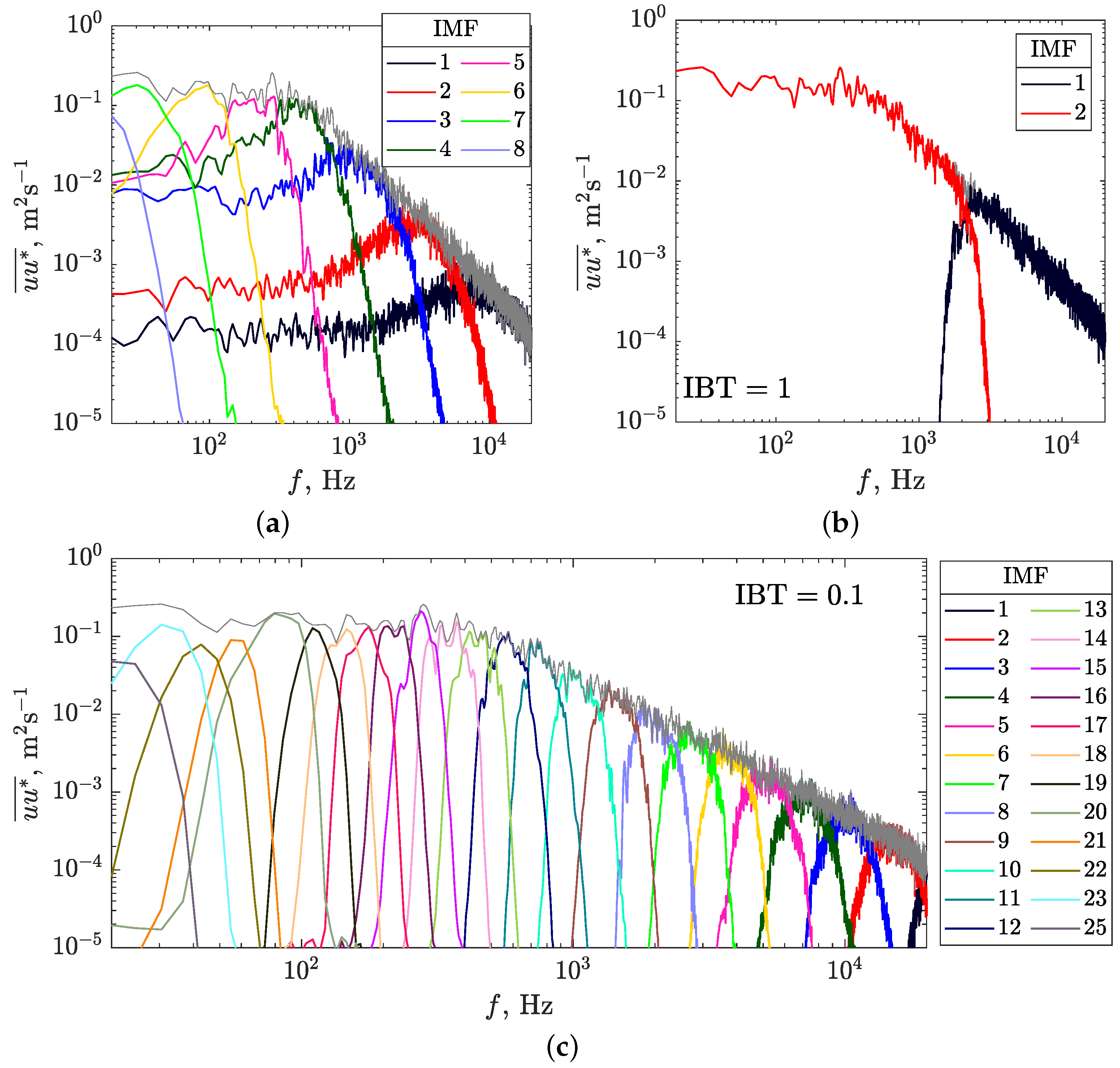
A comparison between the original and the modified EMD is illustrated in Figure 5. The original signal (grey curve) was obtained along the jet lipline and displays the classical flat power at low frequencies and $-5/3$ decay with frequency at the other end of the spectrum. The TVF-EMD data displayed in Figure 5b,c were obtained using instantaneous bandwidth thresholds (IBT) 1 and 0.1, respectively.

The results displayed in Figure 5c are ideal for the present work, as several IMFs of each part of the spectrum can be added up to reconstruct signals representing different characteristic time and length scales. On the basis of the detected phenomena scales, a cut-off filter is defined to separate the decay zone from the energy injection region. These regions were identified using the autospectrum of each of the IMF signals, which were grouped according to their PSD decay with frequency (e.g., flat spectrum for energy-producing region, $-5/3$ decay with frequency for the dissipation region). An $\mathrm{IBT}=0.1$ value was used for the results presented in the paper. Differently from, for example, wavelet analysis, this approach decomposes and reconstructs the signal working only in the frequency domain.

Finally, the results displayed in Figure 5 also indicate that numerical errors associated with the reconstruction of the added-up IMF signals are relatively small. Additionally, decomposed data collected at several locations were compared to their original counterparts, and the resulting PSD levels did not differ by more than 1%. This is well within the expanded uncertainty of the two-point experiment ($\pm 3\%$ [19]). A similar trend was observed for digitally filtered data, discussed in the next section.

3.3. Digital Filters

The shape of the jet streamwise velocity frequency spectrum is well established [3,5]. At high-turbulence regions, the power for individual frequency components is initially ‘flat’ at the low end of the spectrum, followed by a $-5/3$ decay with frequency towards large wavenumbers. Highly intermittent regions are dominated by a signature of the coherent structures, displaying a well-defined energy injection wavenumber range in the form of a ‘hump’.

The single-point time series can be artificially filtered to recreate the signals that produce each of the features discussed above. In the paper, this is done by using digital filters. Investigating the performance of different filter-types is beyond the scope of the present work. A preliminary comparison between infinite impulse response (IIR) and finite impulse response (FIR) filters available as built-in functions in Matlab and Python was carried out. IIR filters required less computational costs and were used for post-processing the data presented in the paper. Both Butterworth and Chebyshev responses were used to set low-pass and high-pass filters.

The frequency attenuation defined for each filter depends upon the jet location analysed and, due to the large dataset, it would have been unfeasible to analyse all spatial domain. Thus, only a few jet points were considered. Nonetheless, the scaling of the data at several regions is demonstrated in the following sections. Thus, it is expected that the filtering process can be extrapolated to other positions.

Using the classical definition, the jet integral time scale was obtained by integrating the autocorrelation coefficients at several jet plume locations. Similarly, a length scale was obtained by integrating the space correlation coefficients. The next sections present the key findings in modelling time scales, convection velocity, and length scale estimation from the single-point statistics.

4. Turbulence Characteristic Time Scales

For jet locations with relatively low intermittency, the normalised autocorrelation coefficients are seen to decay as a one-term exponential function. Based on the lipline data, a universal autocorrelation function defined by the signal time delay, the jet nominal velocity, and the shear layer width is defined as

$$\rho \left(\tau \right)=exp\left(-\frac{\tau U_{\mathrm{j}}}{0.55{\delta }_{\beta }}\right).$$

(3)

This exponential approximation is obtained from fittings applied to autocorrelation coefficients at ten locations along the lipline, and four different jet Mach numbers (ranging from $0.2\le M_{\mathrm{j}}\le 0.8$). A one-term exponential function essentially simplifies the local jet time scale $\mathcal{T}$ to be proportional to $0.55{\delta }_{\beta }/U_{\mathrm{j}}$. The greatest advantage of this simple definition is that characteristic scales of a family of nozzles can be obtained from simple, quick, and low-cost physical or numerical experiments (e.g., experimentally using pressure rake measurements and RANS simulations).

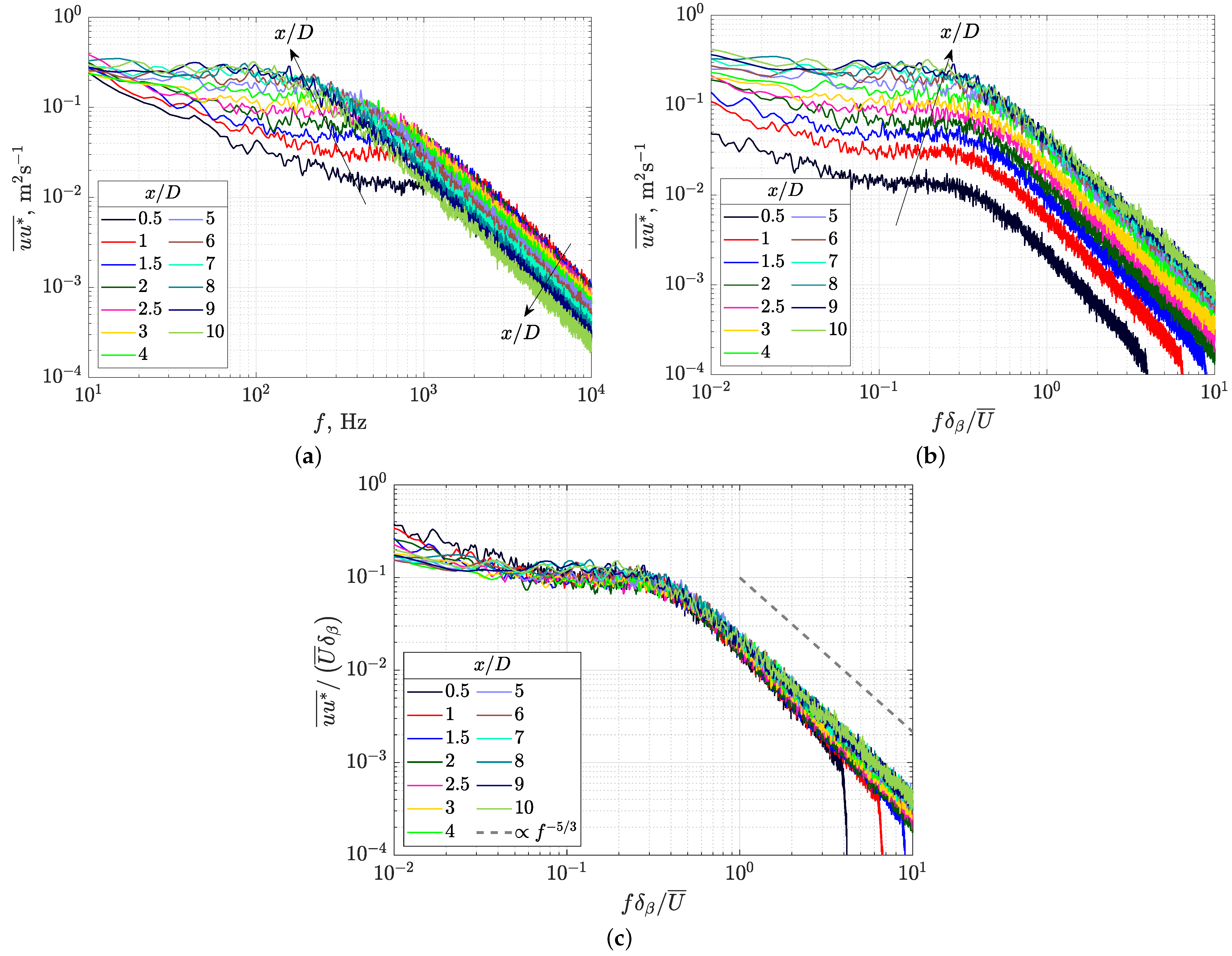
In the frequency domain, a similar function based on the shear layer width and nominal jet velocity can be found. Firstly, scaling of the autospectra measured at several jet plume locations is investigated. Figure 6a displays sample power spectral density (PSD) along the lipline at several axial locations. As expected, the frequency cut-off decreases with increasing axial location, whilst the high-frequency energy content is shifted towards lower frequencies.

Figure 6b,c illustrates the normalisation of the frequency axis, and both frequency and power axes, respectively. Frequency and power are normalised by the shear layer width and jet nominal velocity, as per the autocorrelation function. A good collapse of the data is observed using the aforementioned parameters.

The importance of the result above is twofold. Firstly, a single location in the highly intermittent region is enough to evaluate the single and multi-variate statistics of jet plumes. Secondly, the existence of a well-defined flat region followed by a decay region indicates that the frequency cut-off (i.e., $0.2\le f{\delta }_{\beta }/\overline{U}\le 0.5$) can be inferred from the physical properties of the jet. These two points are central to the rest of the discussion presented below.

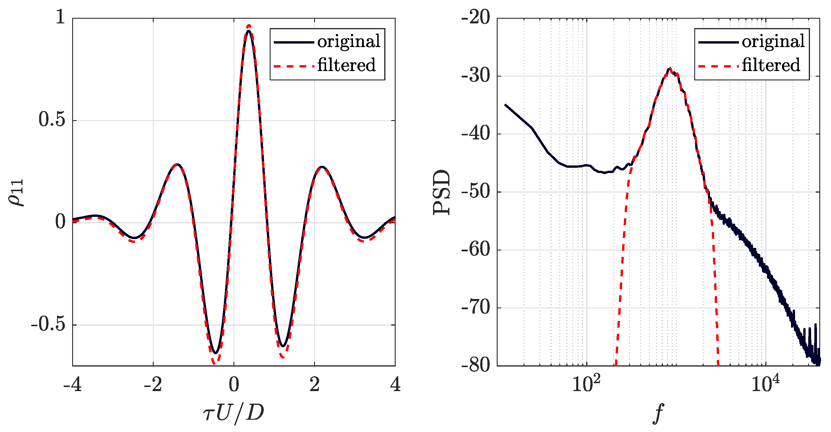
However, it is important to note that the one-term exponential model for the autocorrelation coefficients is not representative of all locations in the jet plume. Within the jet potential core, a sinusoidal component is seen in the autocorrelation and power spectral density functions. This is a signature of the coherent structures existing in the jet shear layer. An example of the autocorrelation and PSD computed on the jet centreline, at $x/D_{\mathrm{j}}=3$, is displayed in Figure 7.

In the figure above, a digitally filtered signal using the filters described in Section 3.3 is also illustrated by red dashed lines. The time signal in the jet low-turbulence-intensity region is dominated by the hump frequencies shown on the right-hand side. Hence, the autocorrelation function (and integral time scale) can be reconstructed. Nonetheless, the limits of the filtering process must be determined by the jet’s physical properties. The standard EMD analysis did not provide a straightforward signal decomposition into well-defined exponential and cosine components. This is one example in which the TVF-EMD works relatively well, although about five times slower than a Chebyshev filter.

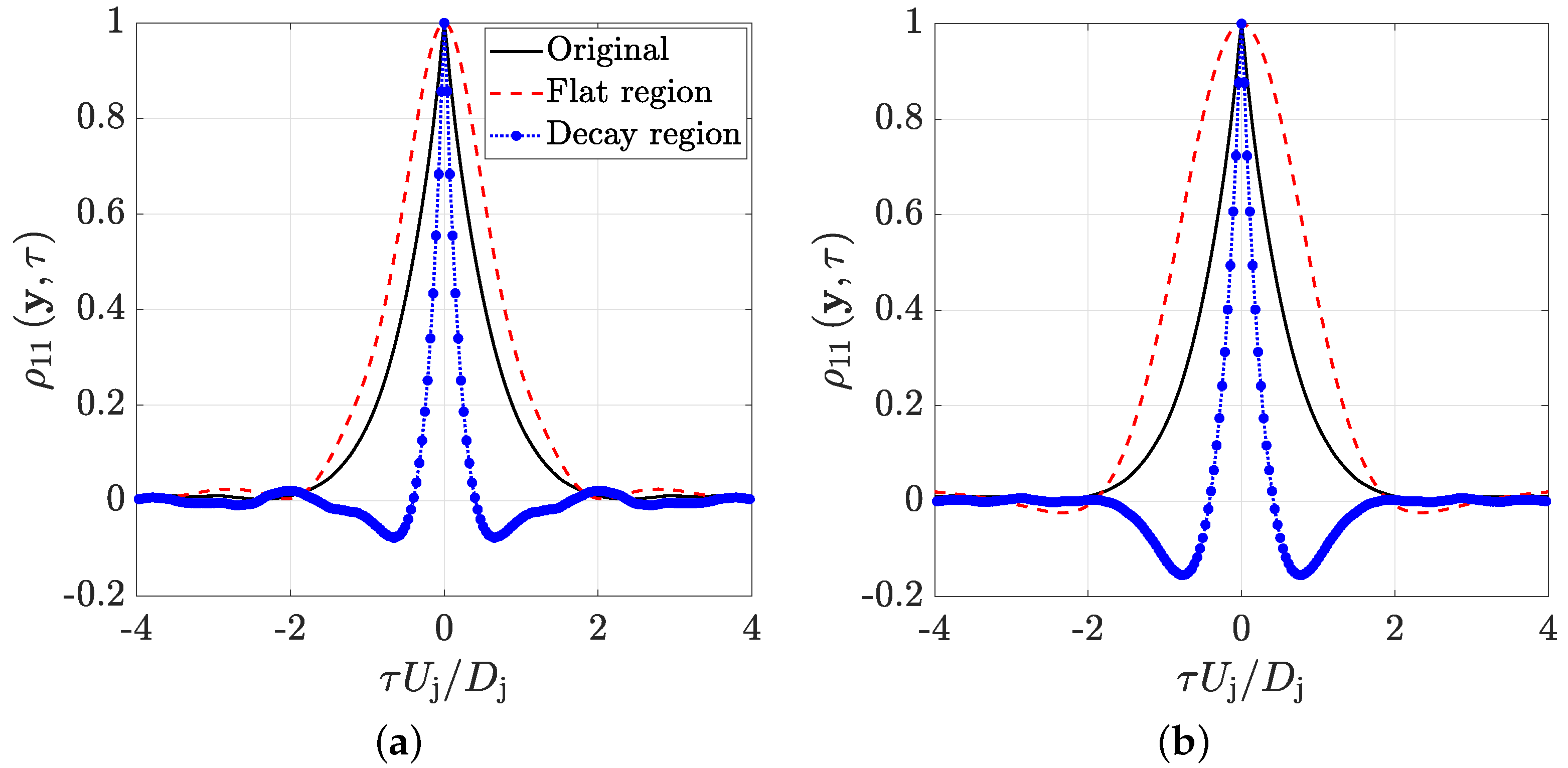
Another problem with the filtering methods regards the definition of the frequency cut-offs. Consider, for example, the filtered signals of Figure 5c. The resulting autocorrelations are displayed in Figure 8. The ‘flat region’ and ‘decay region’ signals were produced by adding up IMF signals. In Figure 8a, only the first ten IMFs were used to produce the decay region curve (a summation of the other IMFs produce the flat region data). Figure 8b used the first 14 IMFs, leaving only the flat region modes for producing the large scale portion of the spectrum.

These results show that, as expected, the signal composed of the decay region in the PSD decays more rapidly than the total signal. The decomposed flat region on the left-hand side is broader than the right-hand-side cut-off. It is clear that tuning this cut-off to match the original signal would generate the same time scales obtained by integrating the autocorrelation coefficients. This then allows the coefficients of the TVF-EMD and digital filter techniques to be used in other regions of the jet plume.

The derivation of these frequency cut-offs is a work in progress and requires additional data to further the current analysis (i.e., different jet nozzle geometries and boundary conditions). At very limited locations, frequency-dependent length-scale models have been presented in the literature [21,22,23]. These models stress that a linear relationship between the single-point and join moments exist in the high-turbulence region.

Approximations of the length scales can, in principle, be obtained from the autocorrelation function and the local eddy convection velocity, $U_{\mathrm{c}}$. These properties are discussed in the next sections.

5. Eddy Convection Velocity

The eddy convection velocity along the jet lipline and centreline was calculated from classical integral scales in the time and frequency domains. A summary of the results is provided below.

5.1. Time Domain

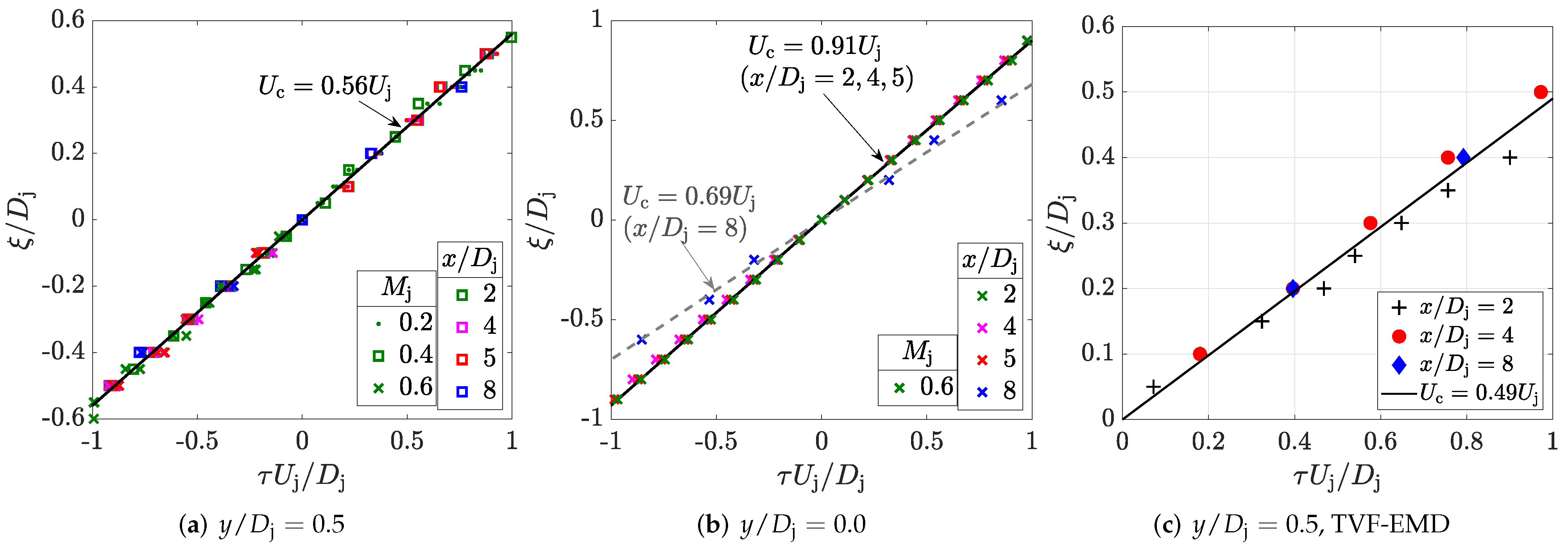
The eddy convection velocity for different jet Mach numbers and jet locations is depicted in Figure 9. Along the lipline, the eddy convection velocity is approximately 56% of the nominal jet velocity. As expected, the eddy convection velocity is larger within the jet’s potential core. Along the centreline the convection velocity decreases rapidly downstream of the end of the potential core. Nonetheless, those values are consistently slightly lower than the local mean flow velocity [5,6].

Figure 9c illustrates the result obtained using the low-frequency part of the signal (i.e., large IMFs) decomposed using the TVF-EMD technique, for IBT = 0.1. The eddy convection velocity calculated at three jet locations collapses relatively well. The $U_{\mathrm{c}}$ obtained from the decomposed signal, however, is seen to be smaller compared to the original data.

The high-frequency signal (summation of the first ten IMFs) produced a convection velocity of 61% of the jet nominal velocity along the lipline. This is an increase of almost 9% compared to the original signal. These differences are discussed further in the next sub-section, as the low-frequency content of the original signal is seen to have a slower velocity than the high-frequency part of the signal.

5.2. Frequency Domain

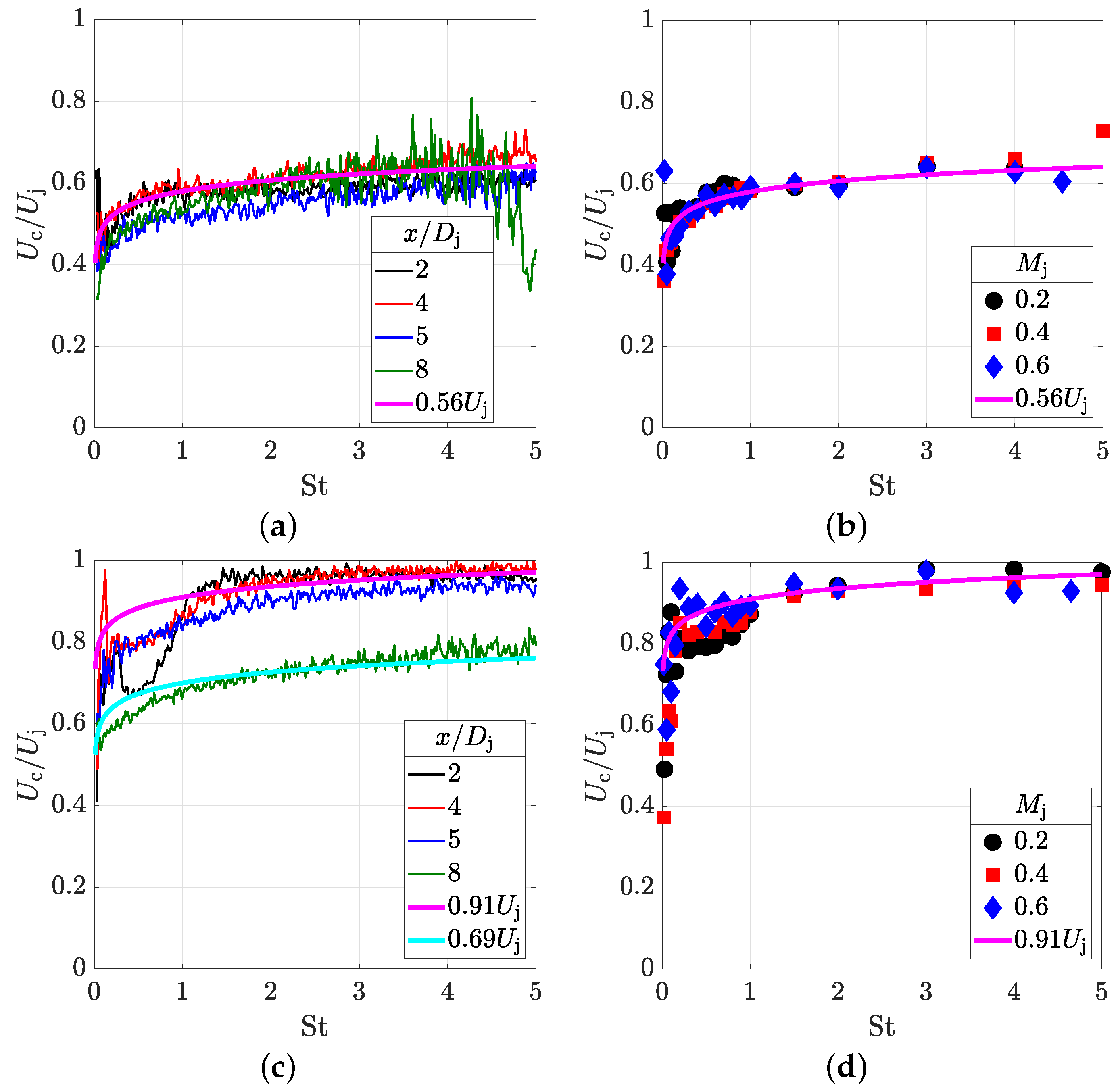
The convection velocity as a function of individual frequency bands was computed. As for the time domain analysis, the frequency-dependent $U_{\mathrm{c}}$ was computed at several axial locations and jet Mach numbers. An example of the results is shown in Figure 10. Data are shown for a reference sensor located at four axial distances, and on the lipline ( Figure 10a) and centreline (Figure 10c). A logarithmic fitting using the Strouhal number based on the jet diameter and nominal velocity is also displayed in all graphs.

The convection velocity is seen to follow a logarithmic relationship with frequency. The wave-like signature in the potential core has a profound effect in the low-frequency region (Figure 10c,d). This effect disappears further downstream on the centreline. This is a potential point for further investigation into modelling characteristic scales within the potential cone.

As mentioned in the previous sub-section, the trends seen in the eddy convection velocity of the filtered data (flat and decay regions of the spectra) agree with the frequency-dependent eddy convection velocity derived from the original signal joint moments. The logarithmic growth with frequency observed in Figure 10 indicates that the signal obtained from the summation of large IMFs removes relatively high-speed components of the data. Normalisation of central moments and joint moments is obtained with the same self-similar parameters. This is demonstrated in the next section.

6. Estimating Length Scales from Time Scales and Eddy Convection Velocity

Similarly to the integral time scales, length scales in the high-turbulence-intensity region can be approximated by a one-term exponential which is function of the shear layer width. This model will, however, be a function of at least five separation directions (i.e., $\pm \xi$, $\pm \eta$ and $\Delta \theta$), as the space and space-time cross-correlation coefficients are not represented by even functions [23]. Additionally, the length scales in the region of high turbulent kinetic energy and the edge of the jet shear layer differ significantly [26].

Nonetheless, time and length scales can be approximated by assuming that the turbulence is frozen, and the power spectral density is well represented by isotropic model functions. This holds true at least in the region of maximum turbulence kinetic energy. Taylor’s hypothesis (limited to the relationship between time and space properties) and isotropic turbulence assumptions are shown to be valid approximations for the statistics of the streamwise velocity component in locations where a quasi-normal distribution is encountered.

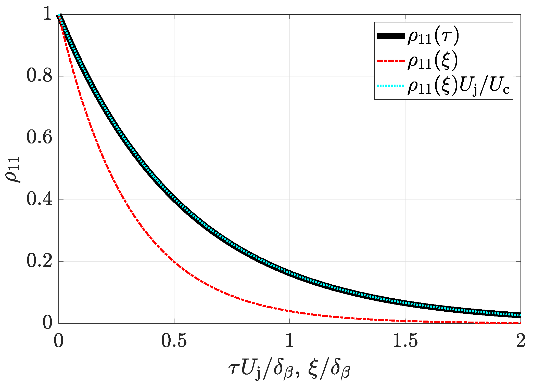
An example result of this hypothesis is illustrated in Figure 11. The autocorrelation coefficients (thick black curve) and the space correlation coefficients (dashed red line) were obtained from the empirical models presented in [23]. Along the lipline, the integral time scale and the integral length scale are related simply by the eddy convection velocity. In turn, the eddy convection velocity is similar to the local mean velocity in that region. Thus, inexpensive and simple single-point experiments can be performed to estimate the characteristic scales along the jet lipline.

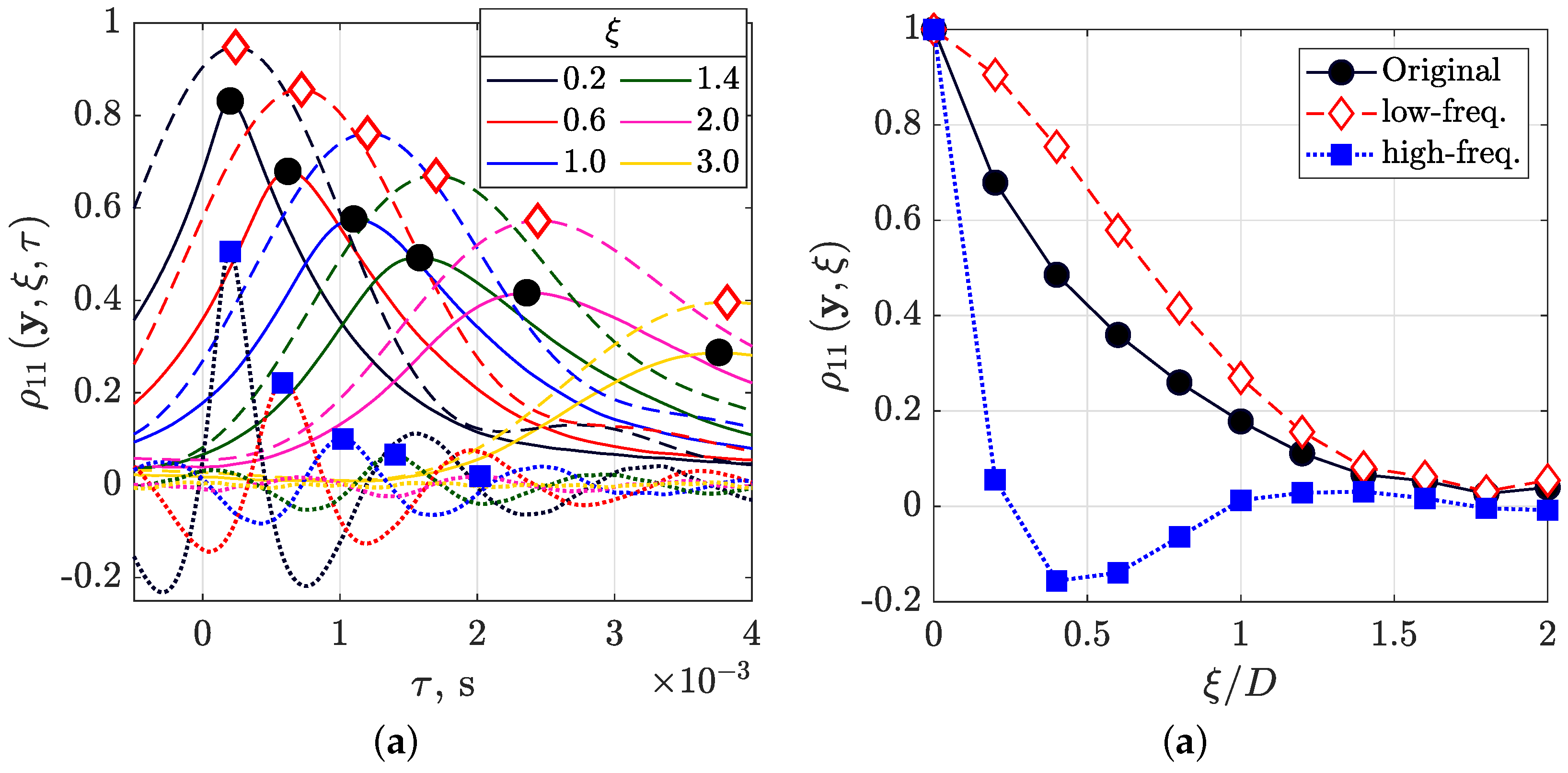
This relationship remains valid for individual frequency bands of the signal. Figure 12a illustrates the space-time cross-correlation coefficients of the original (solid lines) and filtered signals (dashed lines for low-frequency IMFs, dotted lines for high-frequency IMFs). The resulting space coefficients are displayed in Figure 12b. Note that, as the length scale is the area under each curve, the trends observed are similar to the time-scale data provided in Figure 8.

This is not true, however, in other jet locations. The jet plume is truly isotropic, and the frozen hypothesis holds only several dozen diameters downstream of the nozzle exit. Along the centreline, for example, the frozen turbulence hypothesis does not hold. The space correlations do not capture well the periodic oscillation seen in the autocorrelation, and the convection velocity does not correct for the differences in decay of time and space correlations.

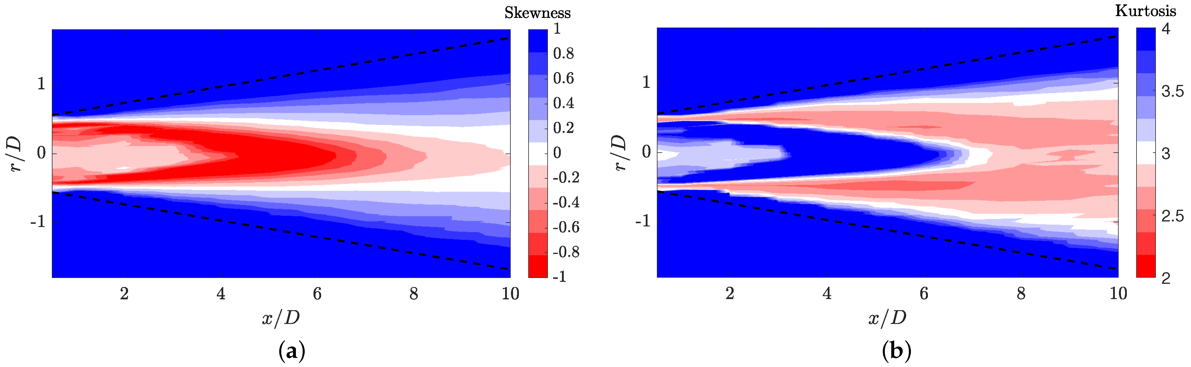
The extent to which the linear relationship between single- and two-point statistics is valid can be estimated by higher-order statistical central moments. Figure 13 displays the third and fourth central moments calculated for an $M=0.6$ jet. A normal distribution (i.e., zero skewness and kurtosis equal to 3) are well represented by the model discussed above. Close to the edge of the shear layer (dashed lines) and the edge of the jet’s potential core, the frozen hypothesis does not hold due to the random behaviour of the small-scale structures and the breakdown of the potential core.

7. Conclusions

This paper described an investigation into the calculation of turbulence integral scales and eddy convection velocity in the flow-field of jets using digital filters and an empirical mode decomposition. The long-term aim of the analyses described is to improve the accuracy of empirical modelling of jet characteristic scales and convection velocity. These unsophisticated, low-cost models are essential to the industrial assessment of new turbofan engine designs installed close to solid surfaces such as wing and high-lift devices.

Single-point and two-point statistics within the highly turbulent shear layer of jets are linearly related by the first statistical central moments. Furthermore, in this region, both central and joint statistical moments are normalised by the physical properties of the jet (i.e., nozzle exit velocity and shear layer width). This is valid for analyses in the time and frequency domain. Although the analysis described here was applied to the highly turbulent region of jet plumes, the filtering approach can be applied to other free shear flows.

Decomposed and reconstructed signals using digital filters and TVF-EMD produced reasonable values of turbulence characteristic scales. The data dominated by low-frequency components travel at a lower convection velocity compared to the original signal. This indicates that the characteristic time scale has a higher increase rate than the characteristic length of large-scale structures. The convection velocity of small-scale structures is higher than that of the complete signal, but the proportion in which time and space scales change with frequency is comparable. The single-point and two-point statistics of the filtered signals were seen to follow similar trends, suggesting that physical insight into the jet turbulence can be extracted even from unphased, pointwise data.

To sum up, digital filters and TVF-EMD can be used as a high-resolution tool to detect flow structures that move at different speeds with the jet flow. These frequency-localized features can then be inputted into stochastic and conditional analyses, which are useful in statistical jet modelling. Both techniques can be applied to small time series and non-stationary data, which provides potential for reducing the costs of numerical simulation and experiments.

References

- Abramovich, G.N. The Theory of Turbulent Jets; The MIT Press Classics: Cambridge, MA, USA, 1963. [Google Scholar]
- Bradshaw, P.; Ferris, D.H.; Johnson, R.H. Turbulence in the noise-producing region of a circular jet. J. Fluid Mech. 1964, 9, 591–624. [Google Scholar] [CrossRef]
- Laurence, J.C. Intensity, Scale, and Spectra of Turbulence in Mixing Region of Free Subsonic Jet (No. NACA-TN-3561). Available online: https://ntrs.nasa.gov/api/citations/19930084270/downloads/19930084270.pdf (accessed on 10 January 2022).
- Hinze, J.O. Turbulence, 2nd ed.; McGraw-Hill: New York, NY, USA, 1975. [Google Scholar]
- Davies, P.O.A.L.; Fisher, M.J.; Barratt, M.J. The Characteristics of the Turbulence in the Mixing Region on a Round Jet. J. Fluid Mech. 1963, 15, 337–367. [Google Scholar] [CrossRef]
- Fisher, M.J.; Davies, P.O.A.L. Correlation measurements in a non-frozen pattern of turbulence. J. Fluid Mech. 1964, 18, 97–116. [Google Scholar] [CrossRef]
- SAE. Gas Turbine Jet Exhaust Noise Prediction SAE ARP 876F; SAE International: Warrendale, PA, USA, 2013. [Google Scholar] [CrossRef]
- ESDU. Computer-based estimation procedure for single-stream jet noise. Including Far-Field, Static Jet Mixing Noise Database for Circular Nozzles—ESDU 98019. (Amendments May 2016). 1998. Available online: https://www.globalspec.com/FeaturedProducts/Detail/ESDU/Computerbased_Estimation_for_Jet_Noise/263965/0 (accessed on 10 January 2022).
- Khavaran, A.; Bridges, J. SHJAR Jet Noise Data and Power Spectral Laws; NASA/TM-2009-21560. 2009. Available online: https://ntrs.nasa.gov/api/citations/20090015382/downloads/20090015382.pdf (accessed on 10 January 2022).
- Batchelor, G.K. The Theory of Homogeneous Turbulence; Cambridge Science Classics: Cambridge, UK, 1982. [Google Scholar]
- Tritton, D. Physical Fluid Dynamics; Oxford Science Publications, Clarendon Press: Oxford, UK, 1988; Chapter 12; p. 12. [Google Scholar]
- Piquet, J. Turbulent Flows—Models and Physics; Springer: Berlin/Heidelberg, Germany, 1999. [Google Scholar] [CrossRef]
- Yule, A.J. Large-scale structure in the mixing layer of a round jet. J. Fluid Mech. 1978, 89, 413–432. [Google Scholar] [CrossRef]
- Lynch, D.A.; Blake, W.K.; Mueller, T.J. Turbulence Correlation Length-Scale Relationships for the Prediction of Aeroacoustic Response. AIAA J. 2005, 43, 1187–1197. [Google Scholar] [CrossRef]
- Kamruzzaman, M.; Lutz, T.; Kraemer, E.; Wuerz, W. On the Length Scales of Turbulence for Aeroacoustic Applications. In Proceedings of the 17th AIAA/CEAS Aeroacoustics Conference (32nd AIAA Aeroacoustics Conference), Portland, OR, USA, 5–8 June 2011. [Google Scholar] [CrossRef]
- Proença, A. Aeroacoustics of Isolated and Installed Jets under Static and in-Flight Conditions. Ph.D. Thesis, University of Southampton, Southampton, UK, 2018. [Google Scholar]
- Karabasov, S.A.; Afsar, M.Z.; Hynes, T.P.; Dowling, A.P.; McMullan, W.A.; Pokora, C.D.; Page, G.J.; McGuirk, J.J. Jet Noise: Acoustic Analogy informed by Large Eddy Simulation. AIAA J. 2010, 48, 1312–1325. [Google Scholar] [CrossRef]
- Wang, Z.N.; Naqavi, I.; Tucker, P.G. Large Eddy Simulation of the Flight Effects on Single Stream Heated Jets. In Proceedings of the 55th AIAA Aerospace Sciences Meeting, Grapevine, TX, USA, 9–13 January 2017. [Google Scholar] [CrossRef]
- Wang, Z.N.; Proenca, A.; Lawrence, J.; Tucker, P.G.; Self, R. Large-Eddy-Simulation Prediction of an Installed Jet Flow and Noise with Experimental Validation. AIAA J. 2020, 58, 2494–2503. [Google Scholar] [CrossRef]
- Self, R.H. Jet noise prediction using the Lighthill acoustic analogy. J. Sound Vib. 2004, 275, 757–768. [Google Scholar] [CrossRef]
- Harper-Bourne, M. Jet noise turbulence measurements. In Proceedings of the 9th AIAA/CEAS Aeroacoustics Conference and Exhibit, Hilton Head, SC, USA, 12–14 May 2003. [Google Scholar]
- Morris, P.J.; Zaman, K. Velocity measurements in jets with application to noise source modeling. J. Sound Vib. 2010, 329, 394–414. [Google Scholar] [CrossRef]
- Proença, A.; Lawrence, J.; Self, R. Measurements of the single-point and joint turbulence statistics of high subsonic jets using hot-wire anemometry. Exp. Fluids 2019, 60, 63. [Google Scholar] [CrossRef] [Green Version]
- Proença, A.; Lawrence, J.; Self, R. Experimental Investigation into the Turbulence Flowfield of In-Flight Round Jets. AIAA J. 2020, 58, 3339–3350. [Google Scholar] [CrossRef]
- Proença, A.; Lawrence, J.; Self, R. Investigation into the turbulence statistics of installed jets using hot-wire anemometry. Exp. Fluids 2020, 61, 220. [Google Scholar] [CrossRef]
- Adam, A.; Papamoschou, D.; Bogey, C. Imprint of Vortical Structures on the Near-Field Pressure of a Turbulent Jet. AIAA J. 2022, 60, 1578–1591. [Google Scholar] [CrossRef]
- Dahl, M.D. Turbulence Statistics for Jet Noise Source Modeling from Filtered PIV Measurements. Int. J. Aeroacoustics 2015, 14, 521–552. [Google Scholar] [CrossRef]
- Gilles, J. Empirical Wavelet Transform. IEEE Trans. Signal Process. 2013, 61, 3999–4010. [Google Scholar] [CrossRef]
- Zeiler, A.; Faltermeier, R.; Keck, I.R.; Tomé, A.M.; Puntonet, C.G.; Lang, E.W. Empirical mode decomposition-an introduction. In Proceedings of the 2010 International Joint Conference on Neural Networks (IJCNN), Barcelona, Spain, 18–23 July 2010; IEEE: Piscataway, NJ, USA, 2010; pp. 1–8. [Google Scholar]
- Debert, S.; Pachebat, M.; Valeau, V.; Gervais, Y. Ensemble-Empirical-Mode-Decomposition method for instantaneous spatial-multi-scale decomposition of wall-pressure fluctuations under a turbulent flow. Exp. Fluids 2010, 50, 339–350. [Google Scholar] [CrossRef]
- Li, H.; Li, Z.; Mo, W. A time varying filter approach for empirical mode decomposition. Signal Process. 2017, 138, 146–158. [Google Scholar] [CrossRef]
Figure 1.
Doak Laboratory Static Jet Rig setup for hot-wire measurements.
Figure 2.
Schematics showing the location of the reference probes (red squares) and the coordinate system of the moving probe (circles). (a) illustration of the jet main regions and location of the reference sensors; (b) example of axial and radial separation traverses.
Figure 3.
Sample data of the cross-correlation coefficients obtained from axial separations along the lipline.
Figure 4.
A sample of IMFs and residual plotted together with the original signal.
Figure 5.
IMFs obtained using the original EMD (a) and modified EMD (b,c).
Figure 6.
PSD measured along the jet’s lipline. (a) absolute data; (b) normalised frequency; and (c) normalised frequency and normalised PSD.
Figure 7.
Example of signal filtering applied to data measured on the jet’s potential core.
Figure 8.
Autocorrelation coefficients of original and decomposed signals measured at , . (a) flat- and decay-region IMFs, (b) only flat-region IMFs.
Figure 9.
Eddy convection velocity calculated from the peak of cross-correlation coefficients using original (a,b) and decomposed (c) wavelet large-scale signals.
Figure 10.
Frequency-dependent eddy convection velocity calculated from the argument of the cross-power spectral density. (a) , , (b) , , (c) , , (d) , .
Figure 11.
Empirical models obtained for the autocorrelation coefficients (black) and space correlation coefficients (red dashed line). The cyan dotted line illustrates the space correlation coefficients obtained using the eddy convection velocity.
Figure 12.
(a) Space-time cross-correlation coefficients and (b) space correlation coefficients of original and filtered signals.
Figure 13.
Higher-order statistics measured for a Mach 0.6 jet. The black dashed lines indicate the edge of the jet shear layer. (a) skewness, (b) kurtosis.
Publisher’s Note: MDPI stays neutral with regard to jurisdictional claims in published maps and institutional affiliations. |
© 2022 by the authors. Licensee MDPI, Basel, Switzerland. This article is an open access article distributed under the terms and conditions of the Creative Commons Attribution (CC BY) license (https://creativecommons.org/licenses/by/4.0/).
Share and Cite
MDPI and ACS Style
Proença, A.R.; Meloni, S. Evaluation of Turbulent Jet Characteristic Scales Using Joint Statistical Moments and an Adaptive Time-Frequency Analysis. Fluids 2022, 7, 125. https://0-doi-org.brum.beds.ac.uk/10.3390/fluids7040125
AMA Style
Proença AR, Meloni S. Evaluation of Turbulent Jet Characteristic Scales Using Joint Statistical Moments and an Adaptive Time-Frequency Analysis. Fluids. 2022; 7(4):125. https://0-doi-org.brum.beds.ac.uk/10.3390/fluids7040125
Chicago/Turabian StyleProença, Anderson R., and Stefano Meloni. 2022. "Evaluation of Turbulent Jet Characteristic Scales Using Joint Statistical Moments and an Adaptive Time-Frequency Analysis" Fluids 7, no. 4: 125. https://0-doi-org.brum.beds.ac.uk/10.3390/fluids7040125