New Dimensionless Number for the Transition from Viscous to Turbulent Flow

Abstract

Within the framework of Classical Continuum Thermomechanics, we consider an unsteady isothermal flow of a simple isotropic linear viscous fluid in the liquid state to investigate the transient flow conditions. Despite the attention paid to this problem by several research works, it seems that the understanding of turbulence in these flow conditions is controversial. We propose a dimensionless procedure that highlights some aspects related to the transition from viscous to turbulent flow which occurs when a finite amplitude pressure wave travels through the fluid. This kind of transition is demonstrated to be described by a (first) dimensionless number, which involves the bulk viscosity. Furthermore, in the turbulent flow regime, we show the role played by a (second) dimensionless number, which involves the turbulent bulk viscosity, in entropy production. Within the frame of the 1D model, we test the performance of the dimensionless procedure using experimental data on the pressure waves propagation in a long pipe (water hammer phenomenon). The obtained numerical results show good agreement with the experimental data. The results’ inspection confirms the predominant role of the turbulent bulk viscosity on energy dissipation processes.

1. Introduction

The physical description of the role of viscous terms for unsteady flows has gained particular attention by researchers. Indeed, this aspect is not related only to theoretical reasoning, while it has a clear practical importance when friction damping deeply influences physical phenomena in engineered structures. The water hammer phenomenon occurring in pipe networks is only one of such examples (e.g., [1]). As it is well known, the water hammer phenomenon plays a crucial role in the pipe’s design and surge protection devices [2]. Generally, the hydraulic approaches to study the water hammer phenomenon are founded on the 1D or 2D models. The classical 1D hydraulic model, in which the friction forces are expressed through the steady approximation, shows a significant discrepancy with the experimental damping and shift pressure waves [1].

Several friction models have been proposed so far. They rely on a series of assumptions that can lead to unreliable reproduction of the physics phenomenon. With reference to the water hammer phenomenon, Ghidaoui et al. [1] highlighted that several models assume that turbulence in pipes is quasi-steady and its features can be modeled as in steady flows. These assumptions have been identified as the main source of unreliability in reproducing experimental findings of transient flows (e.g., [3]).

To overcome this shortcoming, a wide range of friction models are proposed in the literature [3]. The resulting models show an improvement in simulating pressure wave propagation (e.g., [4,5,6,7]); other improvements are obtained with 2D models [8]. The results of most of the models have been compared to experimental data and satisfactory comparison was achieved even if with different assumptions. Mainly developed within the frame of the water hammer problem, some of them assume that the instantaneous value of the viscous term is related to time evolution of the transient [4], some relate the unsteady contribution to the fluid acceleration [9], further conjectured that the role of viscous terms is not longer described by the Reynolds number [10], dimensional analysis of the 1D and 2D models revealed the role of some dimensionless numbers in the pressure wave attenuation in the water hammer phenomenon [3,8,11]. The problem is still controversial and further efforts seem to be needed. It can be observed that while on the one hand some approaches neglect the viscous compressible effects, on the other hand, some proposed dimensionless numbers involve the shear viscosity.

In this paper we emphasize the role played by the viscous compressible effects and the turbulent fluctuations on the energy dissipation processes, proposing new dimensionless numbers that involve the bulk viscosity and turbulent bulk viscosity. A rigorous model is proposed and numerically solved. The obtained results show good agreement with experimental data revealing the reliability of the dimensionless procedure by confirming the predominant role of the turbulent bulk viscosity on energy dissipation processes.

In detail, we consider a simple fluid, i.e., a homogeneous, chemically inert, and electrically neutral fluid, for which the thermodynamic state is defined by an equation of state which relates the absolute temperature, the thermodynamic pressure, and the density [12]. A simple linear viscous fluid is characterized by a linear mechanical constitutive equation; for isotropic fluids, the momentum transport phenomena involve two scalar viscosity coefficients. Using the Classical Continuum Thermomechanics (CCT), we examine an unsteady flow of a simple isotropic linear viscous fluid. In CCT, the mechanical description of fluid flow is based on Newtonian mechanics (with special emphasis on the surface forces), whilst the thermodynamic description is based on Classical Irreversible Thermodynamics, according to which the fluid is in Local Thermodynamic Equilibrium condition (LTE condition). The CCT covers a wide range of phenomena, from Linear non-equilibrium Thermodynamic Regime (LTR), which corresponds to the viscous (laminar) flow regime, to the Non-Linear non-equilibrium Thermodynamic Regime (NLTR), which corresponds to the turbulent flow regime. The LTR, which is stable and regular, is characterized by “small” values of both the velocity gradient, $\parallel \nabla \mathit{v}\parallel$, and the temperature gradient, $\left|\nabla T\right|$: perturbations of the mechanical and thermodynamic state vanish during the evolution of the motion. The NLTR, which is unstable and chaotic, is characterized by “large” values of $\parallel \nabla \mathit{v}\parallel$ and/or $\left|\nabla T\right|$: perturbations amplify and have systematic effects on the motion features. The phenomena which are characterized by very high frequencies and short wavelengths cannot be examined using the CCT, but they require an extended formulation which removes the LTE assumption [13]. Other phenomena, which are very fast or very steep, must be considered as boundary phenomena: these kinds of phenomena can be analyzed using either the CCT or extended formulation.

Within the framework of CCT, ref. [14] have developed an idea suggested by [15,16,17], and they have proposed a 3D model for the unsteady isothermal flow of a simple isotropic linear viscous fluid in the liquid state (i.e., with low compressibility), which involves the turbulent bulk viscosity. In this paper, we re-examine this model. After some brief remarks on the simple isotropic linear viscous fluid (Section 2), we show the connection between the closure equation for the turbulent bulk viscosity and the elementary time scale. For this purpose, Section 3 recalls the main features of the Elementary Scales Method (ESM) [18]. In Section 4, we suggest a dimensionless formulation of the field equations. This procedure allows us to provide new details on the transition from viscous to turbulent flow which occurs when a finite amplitude pressure wave travels through the fluid. We show that this kind of transition is governed by a (first) new dimensionless number, involving the bulk viscosity. In Section 5, we focus on the turbulent flow regime, and we show the role played by a (second) new dimensionless number, involving the turbulent bulk viscosity, on the entropy production. After reducing the 3D model to a 1D model, in Section 6, we show the performance of the dimensionless procedure using experimental data concerning the 1D pressure waves propagation in liquid-filled pipes (water hammer phenomenon). Section 7 closes the paper.

2. Simple Isotropic Linear Viscous Fluids

The momentum transfer due to viscosity occurs in fluids when there is a relative motion between fluid particles [19]. For Simple Isotropic linear viscous Fluids (SIF), the momentum transfer depends only on the first spatial derivative of velocity, and the viscous stress tensor ${\underline{\mathit{T}}}_{vis}$ is expressed by the linear mechanical constitutive equation:

$${\underline{\mathit{T}}}_{vis}=-\eta \left(\nabla ·\mathit{v}\right)\underline{\mathit{I}}-2{\mu }_1{\underline{\mathit{E}}}_{dev}$$

(1)

where $\mathit{v}$ is the velocity, $\underline{\mathit{I}}$ the unit tensor, $\eta =2/3{\mu }_1+{\mu }_2$ the bulk viscosity, ${\mu }_1$ the first viscosity coefficient, ${\mu }_2$ the second viscosity coefficient, ${\underline{\mathit{E}}}_{dev}$ the deviatoric part of the rate of deformation tensor $\underline{\mathit{E}}$, $\underline{\mathit{E}}={\displaystyle \frac{1}{2}}\left(\nabla \mathit{v}+{\nabla \mathit{v}}^T\right)$ the symmetric part of the velocity gradient tensor $\nabla \mathit{v}$. The first viscosity coefficient, and the second viscosity coefficient (and hence the bulk viscosity) are regular functions of $p^a$, the thermodynamic (absolute) pressure, and of T, the absolute temperature. For SIF, the relative velocity ${\mathit{v}}_{rel}$ between two neighboring fluid particles, located in $\mathit{r}$ and in $\mathit{r}+d\mathit{r}$ at the time t, can be expressed as:

$${\mathit{v}}_{rel}=\mathit{v}\left(\mathit{r}+d\mathit{r},t\right)-\mathit{v}\left(\mathit{r},t\right)=\nabla \mathit{v}·d\mathit{r}=\frac{1}{3}\left(\nabla ·\mathit{v}\right)\underline{\mathit{I}}·d\mathit{r}+{\underline{\mathit{E}}}_{dev}·d\mathit{r}+\omega \times d\mathit{r}$$

(2)

where $\omega$ is the angular velocity. Equations (1) and (2) are valid for both LTR and NLTR.

3. Elementary Scales Method (ESM)

Within the framework of CCT, the ESM [18,20] allows us to define the elementary spatial scale $\left|d\mathit{r}\right|$ and the elementary time scale $\left|dt\right|$ such that:

$$\frac{\ell }{\left|d\mathit{r}\right|}\ll 1$$

(3)

$$\frac{t_r}{\left|dt\right|}\ll 1$$

(4)

where ℓ is a fluid molecular length, and $t_r$ the relaxation time, i.e., the interval time to restore an LTE condition in place of a local thermodynamic non-equilibrium condition [19]. The elementary spatial scale can be assumed proportional to the scale of the generic field function gradient [21]:

$$\left|d\mathit{r}\right|\propto \frac{\left|b\right|}{\left|\nabla b\right|}$$

(5)

where b is the generic field function. For the purposes of this paper, we recall that the continuity equation is given as:

$$\frac{\partial \rho }{\partial t}+\nabla ·\left(\rho \mathit{v}\right)=0$$

(6)

where $\rho$ is the density, which assures that $\forall \nabla \mathit{v}\exists dt:\parallel \nabla \mathit{v}dt\parallel \ll 1$. If $\parallel \nabla \mathit{v}dt\parallel \ll 1$, then $det\left(\underline{\mathit{I}}+\nabla \mathit{v}dt\right)=1+\left(\nabla ·\mathit{v}\right)dt$ is very close to 1, and then $\left|\left(\nabla ·\mathit{v}\right)dt\right|\ll 1$. For Simple Isotropic linear viscous Fluids in the Liquid State (SIFLS), for which, in the usual flow conditions, $\epsilon =O\left({10}^9\mathrm{Pa}\right)\gg 1$, where $\epsilon$ is the bulk modulus of elasticity, the differential state equation, expressed as [22]:

$$-\frac{1}{\rho }d\rho =-\frac{1}{\epsilon }d{p}^a+\alpha dT$$

(7)

where $\alpha$ is the thermal expansion, assures that $\forall \nabla T\exists d\mathit{r}:\alpha \left|dT\right|\ll 1$. Observing that $dT={\displaystyle \frac{\partial T}{\partial t}}dt+\nabla T·d\mathit{r}$, the relationship $\alpha \left|dT\right|\ll 1$, formally, implies that $\alpha \left|\nabla T·d\mathit{r}\right|\ll 1$. We stress that the elementary scales $\left|d\mathit{r}\right|$ and $\left|dt\right|$ are regular functions of both space $\mathit{r}$ and time t.

4. Dimensionless Field Equations

To predict the transition from a viscous to turbulent flow regime when a finite amplitude pressure wave travels through SIFLS, we propose a new dimensionless number. For the sake of clarity, this topic is treated by considering adiabatic walls and assuming that the dynamic processes do not change the temperature significantly. By keeping $T=T_0=constant$, the field equations are:

$$\frac{D\rho }{Dt}+\rho \nabla ·\mathit{v}=0$$

(8)

$$\rho \frac{D\mathit{v}}{Dt}=\rho \mathit{f}-\nabla \left(p^a\right)+\nabla \left(\eta \nabla ·\mathit{v}\right)+2\nabla ·\left({\mu }_1{\underline{\mathit{E}}}_{dev}\right)$$

(9)

$$\frac{1}{\rho }d\rho =\frac{1}{\epsilon }d{p}^a$$

(10)

where $\mathit{f}$ is the external body force per unit mass, expressed as $\mathit{f}=-\mathit{g}=-g{\widehat{\mathit{e}}}_z=-g\nabla z$, with $\mathit{g}$ the vector of gravitational acceleration, $g=\left|\mathit{g}\right|$, ${\widehat{\mathit{e}}}_z$ the unit vector in the vertical direction, z the elevation in the gravitational field. In the given flow conditions ($T=T_0=constant$), Equation (7) reduces to the barotropic equation (Equation (10)). Assuming that $\eta$, ${\mu }_1$, $\epsilon$ and $\alpha$ are pressure-independent (Navier–Stokes fluids), the field of relative thermodynamic pressure p can be introduced in place of the absolute pressure $p^a$, being $p=p^a-p_{atm}$, where $p_{atm}$ is the constant atmospheric pressure.

Accordingly, the momentum equation is given as:

$$\rho \frac{D\mathit{v}}{Dt}=-\rho g\nabla z-\nabla p+\eta \nabla \left(\nabla ·\mathit{v}\right)+2{\mu }_1\nabla ·{\underline{\mathit{E}}}_{dev}$$

(11)

the barotropic equation reads as:

$$\rho ={\rho }_0{e}^{p/\epsilon }$$

(12)

and the continuity equation can be expressed as:

$$\frac{1}{\epsilon }\frac{Dp}{Dt}+\nabla ·\mathit{v}=0$$

(13)

where ${\rho }_0=\rho \left(p=0\right)$ is the density at the relative atmospheric pressure. The comparison between Equations (8) and (10), rewritten as:

$$\frac{1}{\rho }\frac{D\rho }{Dt}=\frac{1}{\epsilon }\frac{Dp}{Dt}$$

(14)

provides the continuity equation Equation (13). In order to recast the problem into dimensionless form, in addition to the velocity scale $U_0$ and the length scale $L_0$, a proper pressure scale $p_0$ must be specified. The changes in pressure can be mainly attributed to the perturbation propagation. In the given flow conditions (i.e., isothermal conditions), we express the pressure scale $p_0$, which is identified with the maximum pressure wave amplitude, as:

$$p_0={\rho }_0{c}_0{U}_0$$

(15)

where the relative wave celerity $c_0$ is given as:

$$c_0=\sqrt{\frac{\epsilon }{{\rho }_0}}$$

(16)

Using $c_0$, the time scale $t_0$ is:

$$t_0=\frac{L_0}{c_0}$$

(17)

We stress that the time scale is related to the (fast) perturbation propagation. According to this line of reasoning, setting:

$$b=b_0\left[b\right]$$

(18)

where $b_0$ is the scale of b and the terms in square brackets are dimensionless, we obtain the following relationships:

$$\frac{Db}{Dt}=\frac{\partial b}{\partial t}+\nabla b·\mathit{v}=\frac{b_0{c}_0}{L_0}\left[\frac{\partial b}{\partial t}\right]+\frac{b_0{U}_0}{L_0}\left[\nabla b·\mathit{v}\right]$$

(19)

$$\frac{1}{\rho }\nabla p=\frac{c_0{U}_0}{L_0}\left[\frac{1}{\rho }\nabla p\right]$$

(20)

$$\frac{\eta }{\rho }\nabla \left(\nabla ·\mathit{v}\right)=\frac{\eta U_0}{{\rho }_0{L}_0^2}\left[\frac{1}{\rho }\nabla \left(\nabla ·\mathit{v}\right)\right]$$

(21)

$$\frac{{\mu }_1}{\rho }\nabla ·{\underline{\mathit{E}}}_{dev}=\frac{{\mu }_1{U}_0}{{\rho }_0{L}_0^2}\left[\frac{1}{\rho }\nabla ·{\underline{\mathit{E}}}_{dev}\right]$$

(22)

The adopted notation implies that $\left[B_1{B}_2\right]=\left[B_1\right]\left[B_2\right]$ and $\left[B_1/B_2\right]=\left[B_1\right]/\left[B_2\right]$, where $B_i$ is the generic field function or differential operator. With this setting, Equations (11), (12) and (14) become:

$$\frac{1}{M}\left[\frac{\partial p}{\partial t}\right]+\left[\nabla p·\mathit{v}\right]+\frac{1}{M}\left[\nabla ·\mathit{v}\right]=0$$

(23)

$$\begin{array}{cc}\hfill & \frac{1}{M}\left[\frac{\partial \mathit{v}}{\partial t}\right]+\left[\nabla \mathit{v}·\mathit{v}\right]=-\frac{1}{{Fr}^2}{\widehat{\mathit{e}}}_z-\frac{1}{M}\left[\frac{1}{\rho }\nabla p\right]+\hfill \\ \hfill & \frac{\eta }{{\rho }_0{U}_0{L}_0}\left[\frac{1}{\rho }\nabla \left(\nabla ·\mathit{v}\right)\right]+\frac{2}{Re}\left[\frac{1}{\rho }\nabla ·{\underline{\mathit{E}}}_{dev}\right]\hfill \end{array}$$

(24)

$$\left[\rho \right]=e^{M\left[p\right]}$$

(25)

where $M=U_0/c_0$ is the Mach number, $Fr={\left({\displaystyle \frac{U_0^2}{g{L}_0}}\right)}^{1/2}$ the Froude number, $Re={\displaystyle \frac{{\rho }_0{U}_0{L}_0}{{\mu }_1}}$ the Reynolds number. The term ${\displaystyle \frac{\eta }{{\rho }_0{U}_0{L}_0}}\left[{\displaystyle \frac{1}{\rho }}\nabla \left(\nabla ·\mathit{v}\right)\right]$ is related to the change in density and, in turn, to the change in pressure. Using Equation (15), we derive:

$$\frac{\eta }{{\rho }_0{U}_0{L}_0}\left[\frac{1}{\rho }\nabla \left(\nabla ·\mathit{v}\right)\right]=\frac{c_0\eta }{p_0{L}_0}\left[\frac{1}{\rho }\nabla \left(\nabla ·\mathit{v}\right)\right]$$

(26)

where ${\displaystyle \frac{p_0{L}_0}{c_0\eta }}$ is the new dimensionless number. To our best knowledge, the bulk viscosity is not present in any previous dimensionless number and, consequently, ${\displaystyle \frac{p_0{L}_0}{c_0\eta }}$ cannot be obtained by any combination of existing dimensionless numbers. With Equation (26), the dimensionless momentum equation reads as:

$$\begin{array}{cc}\hfill & \frac{1}{M}\left[\frac{\partial \mathit{v}}{\partial t}\right]+\left[\nabla \mathit{v}·\mathit{v}\right]=-\frac{1}{{Fr}^2}{\widehat{\mathit{e}}}_z-\frac{1}{M}\left[\frac{1}{\rho }\nabla p\right]+\frac{c_0\eta }{p_0{L}_0}\left[\frac{1}{\rho }\nabla \left(\nabla ·\mathit{v}\right)\right]+\hfill \\ \hfill & \frac{2}{Re}\left[\frac{1}{\rho }\nabla ·{\underline{\mathit{E}}}_{dev}\right]\hfill \end{array}$$

(27)

In line with Equation (27), the transition from viscous to turbulent flow regime occurs when $Re$ number and/or ${\displaystyle \frac{p_0{L}_0}{c_0\eta }}$ number exceed their critical values ${Re}_c$ and ${\left({\displaystyle \frac{p_0{L}_0}{c_0\eta }}\right)}_c$, respectively: when $Re>R{e}_c$ and/or ${\displaystyle \frac{p_0{L}_0}{c_0\eta }}>{\left({\displaystyle \frac{p_0{L}_0}{c_0\eta }}\right)}_c$, the stabilizing effect exerted by the viscous forces becomes evanescent and the stable and regular flow turns unstable and chaotic. The two numbers ${\displaystyle \frac{p_0{L}_0}{c_0\eta }}$ and $Re$, which are conceptually similar, are intended to describe different phenomena: the $Re$ number is related to the viscous forces arising from shape variation of the fluid particles; the ${\displaystyle \frac{p_0{L}_0}{c_0\eta }}$ number to the viscous forces arising from volume variation; the $Re$ number governs the transition between the viscous and turbulent regimes during the fluid flow; the ${\displaystyle \frac{p_0{L}_0}{c_0\eta }}$ number the transition which occurs when a pressure wave travels through the fluid, and therefore, a change in density happens. Following the physics of the phenomenon, the higher $p_0$ and $L_0$ and the lower $\eta$ and $c_0$, the higher the ${\displaystyle \frac{p_0{L}_0}{c_0\eta }}$ number.

5. Dimensionless Mean-Flow Field Equations

Following [14], in the turbulent flow regime, the mean-flow equations which correspond to Equations (8)–(10) can be written as follows:

$$\frac{D\rho }{Dt}+\rho \nabla ·\langle \mathit{v}\rangle =0$$

(28)

$$\rho \frac{D〈\mathit{v}〉}{Dt}=-\rho g\nabla z-\nabla \langle p\rangle +\eta \nabla (\nabla ·\langle \mathit{v}\rangle )+2{\mu }_1\nabla ·\langle {\underline{\mathit{E}}}_{dev}\rangle -\nabla ·{\underline{\mathit{T}}}_{Re}$$

(29)

$$\rho ={\rho }_0^{\langle p\rangle /\epsilon }$$

(30)

where:

$$\frac{D\langle b\rangle }{Dt}=\frac{\partial \langle b\rangle }{\partial t}+\nabla \langle b\rangle ·\langle \mathit{v}\rangle$$

(31)

and:

$${\underline{\mathit{T}}}_{Re}=\rho \langle {\mathit{v}}^{\prime }\otimes {\mathit{v}}^{\prime }\rangle$$

(32)

is the Reynolds stress tensor. Equations (28)–(30) can be obtained using the Reynolds decomposition along with the Russo Spena Assumption (RSAss) [14] setting:

$$p\left(\mathit{r},t\right)=\langle p(\mathit{r},t)\rangle +p^{\prime }(\mathit{r},t)$$

(33)

$$\mathit{v}\left(\mathit{r},t\right)=\langle \mathit{v}(\mathit{r},t)\rangle +{\mathit{v}}^{\prime }(\mathit{r},t)$$

(34)

$$\rho \left(\mathit{r},t\right)=\langle \rho (\mathit{r},t)\rangle$$

(35)

$${\rho }^{\prime }\left(\mathit{r},t\right)=0$$

(36)

where $\langle b(\mathit{r},t)\rangle$ and $b^{\prime }\left(\mathit{r},t\right)$ are the ensemble-mean and the turbulent fluctuation of the generic field function b, respectively.

It has to be stressed that the density fluctuations are assumed to be negligible, whilst its mean value can vary depending on the mean value of the pressure, according to Equation (30).

In agreement with RSAss, the differential form of the mean barotropic equation can be expressed as:

$$\frac{1}{\rho }d\rho =\frac{1}{\epsilon }d\langle p\rangle$$

(37)

According to Equation (37), the mean-flow equation which corresponds to Equation (14) reads as follows:

$$\frac{1}{\rho }\frac{D\rho }{Dt}=\frac{1}{\epsilon }\frac{D\langle p\rangle }{Dt}$$

(38)

The comparison between Equations (28) and (38) leads to:

$$\frac{1}{\epsilon }\frac{D\langle p\rangle }{Dt}+\nabla ·\langle \mathit{v}\rangle =0$$

(39)

In the context of the eddy-viscosity model, Equation (29) is consistent with the relationship:

$$\langle {\mathit{v}}_{rel}\rangle =\langle \mathit{v}(\mathit{r}+d\mathit{r},t)\rangle -\langle \mathit{v}(\mathit{r},t)\rangle =\nabla \langle \mathit{v}\rangle ·\langle d\mathit{r}\rangle +\langle \nabla {\mathit{v}}^{\prime }·d{\mathit{r}}^{\prime }\rangle$$

(40)

being $d\mathit{r}=\langle d\mathit{r}\rangle +d{\mathit{r}}^{\prime }$ (as a field function and in line with the Reynolds decomposition, $d\mathit{r}$ can be splitted in the ensemble-mean value, $\langle d\mathit{r}\rangle$, and in the fluctuation value, $d{\mathit{r}}^{\prime }$). Equation (40) can be deduced from Equation (2) setting:

$$\begin{array}{cc}\hfill & {\mathit{v}}_{rel}=\mathit{v}\left(\mathit{r}+d\mathit{r},t\right)-\mathit{v}\left(\mathit{r},t\right)=\nabla \mathit{v}·d\mathit{r}=\hfill \\ \hfill & \nabla \langle \mathit{v}\rangle ·\langle d\mathit{r}\rangle +\nabla \langle \mathit{v}\rangle ·d{\mathit{r}}^{\prime }+\nabla {\mathit{v}}^{\prime }·\langle d\mathit{r}\rangle +\nabla {\mathit{v}}^{\prime }·d{\mathit{r}}^{\prime }\hfill \end{array}$$

(41)

According to Equation (41), $\langle {\underline{\mathit{T}}}_{vis}\rangle$ is related to $\nabla \langle \mathit{v}\rangle$ by means of the relationship:

$$\langle {\underline{\mathit{T}}}_{vis}\rangle =-\eta \left(\nabla ·\langle \mathit{v}\rangle \right)\underline{\mathit{I}}-2{\mu }_1\langle {\underline{\mathit{E}}}_{dev}\rangle$$

(42)

while ${\underline{\mathit{T}}}_{Re}$ is linked to turbulent fluctuations.

In the CCT context, the ESM assures that $\forall \nabla \langle \mathit{v}\rangle \exists \langle dt\rangle :t_r/\left|\langle dt\rangle \right|\ll 1$ and $\parallel \nabla \langle \mathit{v}\rangle \langle dt\rangle \parallel \ll 1$, being $dt=\langle dt\rangle +d{t}^{\prime }$ (as for $d\mathit{r}$, the field function $dt$ is splitted in the ensemble-mean value, $\langle dt\rangle$, and in the fluctuation value, $d{t}^{\prime }$). If $\parallel \nabla \langle \mathit{v}\rangle \langle dt\rangle \parallel \ll 1$ also $|\left(\nabla ·\langle \mathit{v}\rangle \right)\langle dt\rangle |\ll 1$.

The additional Reynolds stress tensor ${\underline{\mathit{T}}}_{Re}$ can be decomposed into its isotropic and deviatoric parts:

$${\underline{\mathit{T}}}_{Re}={\left({\underline{\mathit{T}}}_{Re}\right)}_{iso}+{\left({\underline{\mathit{T}}}_{Re}\right)}_{dev}$$

(43)

The deviatoric stress tensor ${\left({\underline{\mathit{T}}}_{Re}\right)}_{dev}$ is related to additional shear stresses; the isotropic part ${\left({\underline{\mathit{T}}}_{Re}\right)}_{iso}$, which is related to additional relative normal stresses, can be expressed using the constitutive equation [14]:

$${\left({\underline{\mathit{T}}}_{Re}\right)}_{iso}=-{\eta }_{tur}\left(\nabla ·\langle \mathit{v}\rangle \right)\underline{\mathit{I}}$$

(44)

where the turbulent bulk viscosity ${\eta }_{tur}$, which depends on both the fluid and the kinematic properties of the flow field, is expressed by the closure equation:

$${\eta }_{tur}={\eta }_{tur}\left(\mathit{r},t\right)=\lambda e^{|\left(\nabla ·\langle \mathit{v}\rangle \right)\langle dt\rangle |}$$

(45)

where $\lambda$ is a parameter. Equation (45), which represents more accurately the closure equation proposed in [14], shows the connection between the turbulent bulk viscosity and the elementary time scale. If the temperature changes due to the dynamic processes, in agreement with the RSAss, by assuming $\alpha =constant$ and $\epsilon =constant$, the mean state equation is:

$$\alpha \langle dT\rangle =-\frac{1}{\rho }d\rho +\frac{1}{\epsilon }d\langle p^a\rangle =\left(\nabla ·\langle \mathit{v}\rangle \right)\langle dt\rangle +\frac{1}{\epsilon }d\langle p^a\rangle$$

(46)

According to Equation (46), assuming for SIFLS that $\epsilon =O\left({10}^9\mathrm{Pa}\right)\gg 1$, the ESM assures that $|d\langle p^a\rangle |/\epsilon \ll 1$, $|\left(\nabla ·\langle \mathit{v}\rangle \right)\langle dt\rangle |\ll 1$, $\alpha |d\langle T\rangle |\ll 1$. Setting $d\langle T\rangle ={\displaystyle \frac{\partial \langle T\rangle }{\partial t}}\langle dt\rangle +\nabla \langle T\rangle ·\langle d\mathit{r}\rangle$, the relationship $\alpha \left|d\langle T\rangle \right|\ll 1$ implies that $\forall \nabla \langle T\rangle \exists \langle d\mathit{r}\rangle :\ell /|\langle d\mathit{r}\rangle |\ll 1$ and $\alpha \left|\nabla \langle T\rangle ·\langle d\mathit{r}\rangle \right|\ll 1$.

With Equations (43) and (44), Equation (29) becomes:

$$\begin{array}{cc}\hfill & \rho \frac{D\langle \mathit{v}\rangle }{Dt}=-\rho g\nabla z-\nabla \langle p\rangle +\eta \nabla (\nabla ·\langle \mathit{v}\rangle )+\nabla ({\eta }_{tur}\nabla ·\langle \mathit{v}\rangle )+\hfill \\ \hfill & 2{\mu }_1\nabla ·\langle {\underline{\mathit{E}}}_{dev}\rangle -\nabla ·{\left({\underline{\mathit{T}}}_{Re}\right)}_{dev}\hfill \end{array}$$

(47)

In agreement with Equation (47), the mean kinetic energy equation is given as:

$$\rho \frac{D\langle k\rangle }{Dt}=-\rho g\nabla z·\langle \mathit{v}\rangle -\nabla \langle p\rangle ·\langle \mathit{v}\rangle -(\nabla ·\langle \widetilde{\underline{\mathit{T}}}\rangle )·\langle \mathit{v}\rangle$$

(48)

where $\langle k\rangle =\langle v^2\rangle /2$ is the ensemble-mean specific kinetic energy, and:

$$\langle \widetilde{\underline{\mathit{T}}}\rangle =\langle {\underline{\mathit{T}}}_{vis}\rangle +{\underline{\mathit{T}}}_{Re}$$

(49)

In the given flow conditions ($T=T_0=constant$), the mean energy equation is:

$$\rho \frac{D\langle e\rangle }{Dt}=-\rho g\nabla z·\langle \mathit{v}\rangle -\nabla ·\left(\langle p\rangle \langle \mathit{v}\rangle \right)+\nabla ·(\langle \widetilde{\underline{\mathit{T}}}\rangle ·\langle \mathit{v}\rangle )$$

(50)

where $\langle e\rangle =\langle k\rangle +\langle u_i\rangle$, with $\langle u_i\rangle$ ensemble-mean specific internal energy. The mean internal energy equation:

$$\rho \frac{D〈u_i〉}{Dt}=-\langle p\rangle \nabla ·\langle \mathit{v}\rangle -\langle \tilde{\mathit{T}}\rangle :\nabla \langle \mathit{v}\rangle$$

(51)

in connection with the mean Gibbs equation:

$$d〈u_i〉=Td\langle s\rangle +\frac{\langle p\rangle }{\rho }d\rho$$

(52)

provides the mean entropy equation:

$$\begin{array}{cc}\hfill & \rho T\frac{D\langle s\rangle }{Dt}=-\langle \tilde{\mathit{T}}\rangle :\nabla \langle \mathit{v}\rangle =\left(\eta +{\eta }_{tur}\right){(\nabla ·\langle \mathit{v}\rangle )}^2-\langle {\underline{\tilde{\mathit{T}}}}_{dev}\rangle :\langle {\underline{\mathit{E}}}_{dev}\rangle =\hfill \\ \hfill & \left(\eta +{\eta }_{tur}\right){(\nabla ·\langle \mathit{v}\rangle )}^2+2{\mu }_1\langle {\underline{\mathit{E}}}_{dev}\rangle :\langle {\underline{\mathit{E}}}_{dev}\rangle -{\left({\underline{\mathit{T}}}_{Re}\right)}_{dev}:\langle {\underline{\mathit{E}}}_{dev}\rangle \hfill \end{array}$$

(53)

where $\langle s\rangle$ is the ensemble-mean specific entropy and $\langle {\underline{\tilde{\mathit{T}}}}_{dev}\rangle$ the deviatoric part of $\langle \underline{\tilde{\mathit{T}}}\rangle$. Setting:

$$\begin{array}{cc}\hfill & \frac{1}{\rho }\nabla \left({\eta }_{tur}\nabla ·\langle \mathit{v}\rangle \right)=\frac{{\eta }_{tur}}{\rho }\nabla \left(\right|\left(\nabla ·\langle \mathit{v}\rangle \right)\langle dt\rangle \left|\right)\nabla ·\langle \mathit{v}\rangle +\frac{{\eta }_{tur}}{\rho }\nabla (\nabla ·\langle \mathit{v}\rangle )=\hfill \\ \hfill & \frac{{\eta }_{tur}{U}_0^2}{{\rho }_0{c}_0{L}_0^2}\left[\frac{1}{\rho }\nabla \left(\right|\left(\nabla ·\langle \mathit{v}\rangle \right)\langle dt\rangle \left|\right)\nabla ·\langle \mathit{v}\rangle \right]+\frac{{\eta }_{tur}{U}_0}{{\rho }_0{L}_0^2}\left[\frac{1}{\rho }\nabla (\nabla ·\langle \mathit{v}\rangle )\right]\hfill \end{array}$$

(54)

$$\frac{1}{\rho }\nabla ·{\left({\underline{\mathit{T}}}_{Re}\right)}_{dev}=\frac{U_0^2}{L_0}\left[\frac{1}{\rho }\nabla ·{\left({\underline{\mathit{T}}}_{Re}\right)}_{dev}\right]$$

(55)

$$T\langle s\rangle =U_0^2\left[T\langle s\rangle \right]$$

(56)

$$T\frac{\mathrm{D}\langle s\rangle }{\mathrm{D}t}=\frac{U_0^2{c}_0}{L_0}\left[T\frac{\partial \langle s\rangle }{\partial t}\right]+\frac{U_0^3}{L_0}[T\nabla \langle s\rangle ·\langle \mathit{v}\rangle ]$$

(57)

the dimensionless form of momentum and entropy equations read as follows:

$$\begin{array}{cc}\hfill & \frac{1}{M}\left[\frac{\partial \langle \mathit{v}\rangle }{\partial t}\right]+[\nabla \langle \mathit{v}\rangle ·\langle \mathit{v}\rangle ]=-\frac{1}{F{r}^2}{\widehat{\mathit{e}}}_z-\frac{1}{M}\left[\frac{1}{\rho }\nabla \langle p\rangle \right]+\frac{c_0\eta }{p_0{L}_0}\left[\frac{1}{\rho }\nabla (\nabla ·\langle \mathit{v}\rangle )\right]+\hfill \\ \hfill & \frac{2}{Re}\left[\frac{1}{\rho }\nabla ·\langle {\underline{\mathit{E}}}_{dev}\rangle \right]+M\frac{c_0{\eta }_{tur}}{p_0{L}_0}\left[\frac{1}{\rho }\nabla \left(\right|\left(\nabla ·\langle \mathit{v}\rangle \right)\langle dt\rangle \left|\right)\nabla ·\langle \mathit{v}\rangle \right]+\hfill \\ \hfill & \frac{c_0{\eta }_{tur}}{p_0{L}_0}\left[\frac{1}{\rho }\nabla (\nabla ·\langle \mathit{v}\rangle )\right]-\left[\frac{1}{\rho }\nabla ·{\left({\underline{\mathit{T}}}_{Re}\right)}_{dev}\right]\hfill \end{array}$$

(58)

$$\begin{array}{cc}\hfill & \frac{1}{M}\left[T\frac{\partial \langle s\rangle }{\partial t}\right]+[T\nabla \langle s\rangle ·\langle \mathit{v}\rangle ]=\frac{c_0\eta }{p_0{L}_0}\left[\frac{1}{\rho }{(\nabla ·\langle \mathit{v}\rangle )}^2\right]+\frac{c_0{\eta }_{tur}}{p_0{L}_0}\left[\frac{1}{\rho }{(\nabla ·\langle \mathit{v}\rangle )}^2\right]+\hfill \\ \hfill & \frac{2}{Re}\left[\frac{1}{\rho }\langle {\underline{\mathit{E}}}_{dev}\rangle :\langle {\underline{\mathit{E}}}_{dev}\rangle \right]-\left[\frac{1}{\rho }{\left({\underline{\mathit{T}}}_{Re}\right)}_{dev}:\langle {\underline{\mathit{E}}}_{dev}\rangle \right]\hfill \end{array}$$

(59)

where ${\displaystyle \frac{p_0{L}_0}{c_0{\eta }_{tur}}}$ is the (second) new dimensionless number.

6. Test Case

In order to test the performance of the dimensionless procedure, we focus on the classical hydraulic problem of 1D finite amplitude pressure waves propagation in liquid-filled pipe (water hammer phenomenon). This phenomenon, which involves rapid changes in a liquid density and considerable energy dissipations, occurs in pipe networks as a result of valve maneuvers: the local liquid velocity variations generate pressure waves that travel in the liquid-pipe system. In a 1D context, for a horizontal single-pipe system with axially symmetric geometry, Equations (30), (39), (47), and (53) become:

$$\frac{1}{\epsilon }\frac{\partial p}{\partial t}+\frac{1}{\epsilon }U\frac{\partial p}{\partial x}+\frac{\partial U}{\partial x}=0$$

(60)

$$\frac{\partial U}{\partial t}+U\frac{\partial U}{\partial x}=-\frac{1}{\rho }\frac{\partial p}{\partial x}+\frac{\eta }{\rho }\frac{{\partial }^{2}U}{\partial x^2}-f\frac{U\left|U\right|}{2D}+\frac{1}{\rho }\frac{\partial }{\partial x}\left({\eta }_{tur}\frac{\partial U}{\partial x}\right)$$

(61)

$$\rho ={\rho }_0{e}^{p/\epsilon }$$

(62)

$$T\frac{\partial s}{\partial t}+TU\frac{\partial s}{\partial x}=\frac{\left(\eta +{\eta }_{tur}\right)}{\rho }{\left(\frac{\partial U}{\partial x}\right)}^2+f\frac{U^2\left|U\right|}{2D}$$

(63)

where x is the pipe-axis longitudinal coordinate (i.e., along the mean flow direction), $\rho =\rho \left(x,t\right)$ the liquid density, $U=U\left(x,t\right)=Q\left(x,t\right)/\Omega$ the ensemble-mean value of the relative velocity of the liquid with respect to the solid wall, with $Q\left(x,t\right)$ the ensemble-mean volumetric flow rate and $\Omega$ the (constant) area of the pipe cross-section, $p=p\left(x,t\right)$ the ensemble-mean value of the pressure, D the (constant) pipe diameter, f the Darcy friction factor. It should be underlined that the temperature T is a parameter of the problem.

The parameter $\epsilon$ depends on the pipe-liquid system; the parameters f and ${\eta }_{tur}$ depend on both the pipe-liquid system and the kinematic property of the flow field. In the crossover from 3D to 1D, the velocity $\langle \mathit{v}\rangle$ is reduced to U; the term $2{\displaystyle \frac{{\mu }_1}{\rho }}\nabla ·\langle {\underline{\mathit{E}}}_{dev}\rangle -\frac{1}{\rho }\nabla ·{\left({\underline{\mathit{T}}}_{Re}\right)}_{dev}$ is reduced to $-f{\displaystyle \frac{U\left|U\right|}{2D}}$; the term $-{\displaystyle \frac{1}{\rho }}\langle {\widetilde{\underline{\mathit{T}}}}_{dev}\rangle :\langle {\underline{\mathit{E}}}_{dev}\rangle$ is reduced to $-f{\displaystyle \frac{U^2\left|U\right|}{2D}}$; the material derivative ${\displaystyle \frac{D\langle b\rangle }{Dt}}$ is reduced to ${\displaystyle \frac{\partial b}{\partial t}}+U{\displaystyle \frac{\partial b}{\partial x}}$; the term $\left|\left(\nabla ·\langle \mathit{v}\rangle \right)\langle dt\rangle \right|$ is reduced to $\left|{\displaystyle \frac{\partial U}{\partial x}}dt\right|$ and the closure equation (i.e., Equation (45)) becomes:

$${\eta }_{tur}={\eta }_{tur}\left(x,t\right)=\lambda e^{\left|\frac{\partial U}{\partial x}dt\right|}$$

(64)

According to system of Equations (60)–(62), which neglect the thermal effects, cavitation phenomena, and assume an elastic behavior of the pipe-wall, the relative wave celerity reads as follows:

$$c=\sqrt{\frac{\epsilon }{{\rho }_0}{e}^{-p/\epsilon }}$$

(65)

The unknown parameters $\epsilon$ and $\lambda$ must be calibrated using experimental data. The experimental data considered herein available in the literature [23], consist of thermodynamic pressure time series, expressed in terms of piezometric head $h\left(x,t\right)={\displaystyle \frac{p}{{\rho }_{0}g}}$, collected at the downstream section of a high density polyethylene pipe (in $x=X$, where $X=164.93$ m is the pipe length, with $D=93.3$ mm, wall thickness $8.1$ mm), during the water hammer phenomenon (${\rho }_0$ = 1000 kg/m${}^3$). The experiments are carried out using standard laboratory facilities (reservoir-pump-pressurized tank-pipe-valve): the pipe connects the upstream pressurized tank to a downstream maneuver valve; the piezometric signals are measured employing piezoresistive transducers, the steady-state discharge by means of electromagnetic flow-meters. Once the initial steady-state is established, the water hammer is generated by a fast closure of the valve. During the tests, the water temperature range varied between 18.1 and 18.9 ${}^{\circ }$C. Hence, the basic hypothesis of the proposed model (i.e., isothermal flow) applies. Details about experimental set-up and procedures are in [23].

Table 1. Initial steady-state conditions.

Test	$\mathit{U}(\mathit{x},0)$ = ${\mathit{U}}_0\mathbf{m}/\mathbf{s}$	$\mathit{h}(\mathit{X},0)\mathbf{m}$	$\mathbf{Re}={\displaystyle \frac{{\mathit{\rho }}_0{\mathit{U}}_0\mathit{D}}{{\mathit{\mu }}_1}}$
1	0.07	21.20	6940
2	0.14	21.03	13,345
3	0.22	20.80	20,526
4	0.24	20.68	22,392
5	0.31	20.51	28,923
6	0.36	20.37	33,588
7	0.42	20.04	39,653
8	0.52	19.61	48,143
9	0.58	19.47	54,114
10	0.66	19.39	61,578
11	0.71	19.11	66,710
12	0.78	18.92	72,774

summarizes the experimental initial steady-state conditions. Figure 1 shows the experimental results (for the clarity of the plot, the time series are shifted vertically by 40 m, horizontally by 0.35 s; the duration of the observation time, $t_d$, is 10 s). The maximum surge pressure $\Delta p_{max}$ is in agreement with the Joukowsky formula:

$$\Delta p_{max}={\rho }_0{c}_0{U}_0=p_0$$

(66)

where $\Delta p=p\left(X,t\right)-p\left(X,0\right)$

As shown in Figure 2, the experimental trials collapse in a master curve if the data are scaled setting $\left[p\right]={\displaystyle \frac{gh}{c_0{U}_0}}$, $g=9.81$ m/s${}^2$, $c_0=350$ m/s, $L_0$ = $D=93.5$ mm, $t_d=10$ s. This result can be attributed to the reliability of the dimensionless procedure and indicates no significant Reynolds number dependence, in agreement with [14]. The selected value of $c_0$ assures that $\left[\Delta p\right]=\left[p\left(X,t\right)\right]-\left[p\left(X,0\right)\right]\simeq 1$ for $0<\left[t/t_d\right]\le$ 0.1; with this setting, $\epsilon ={\rho }_0{c}_0^2=$1.225 × 10${}^8$ Pa. The dimensionless form of Equations (60)–(63) becomes:

$$\frac{1}{M}\left[\frac{\partial p}{\partial t}\right]+\left[U\frac{\partial p}{\partial x}\right]+\frac{1}{M}\left[\frac{\partial U}{\partial x}\right]=0$$

(67)

$$\begin{array}{cc}\hfill & \frac{1}{M}\left[\frac{\partial U}{\partial t}\right]+\left[U\frac{\partial U}{\partial x}\right]=-\frac{1}{M}\left[\frac{1}{\rho }\frac{\partial p}{\partial x}\right]+\frac{c_0\eta }{p_0{L}_0}\left[\frac{1}{\rho }\frac{{\partial }^{2}U}{\partial x^2}\right]-\frac{f}{2}\left[U\left|U\right|\right]+\hfill \\ \hfill & \frac{c_0{\eta }_{tur}}{p_0{L}_0}\left[\frac{1}{\rho }\frac{{\partial }^{2}U}{\partial x^2}\right]+M\frac{c_0{\eta }_{tur}}{p_0{L}_0}\left[\frac{1}{\rho }\frac{\partial }{\partial x}\left(\left|\frac{\partial U}{\partial x}dt\right|\right)\frac{\partial U}{\partial x}\right]\hfill \end{array}$$

(68)

$$\left[\rho \right]=e^{M\left[p\right]}$$

(69)

$$\begin{array}{cc}\hfill & \frac{1}{M}\left[T\frac{\partial s}{\partial t}\right]+\left[TU\frac{\partial s}{\partial x}\right]=\frac{c_0\eta }{p_0{L}_0}\left[\frac{1}{\rho }{\left(\frac{\partial U}{\partial x}\right)}^2\right]+\hfill \\ \hfill & \frac{c_0{\eta }_{tur}}{p_0{L}_0}\left[\frac{1}{\rho }{\left(\frac{\partial U}{\partial x}\right)}^2\right]+\frac{f}{2}\left[U^2\left|U\right|\right]\hfill \end{array}$$

(70)

Equations (67)–(69) are solved using a commercial finite element software package [24]. Following [14], the elementary time scale $\left|dt\right|$ is chosen proportionalyl to the wave travel time through the pipe $t_w$. In a first step, $t_w$ can be approximated as:

$$t_w=\frac{2X}{c_0}$$

(71)

The numerical simulations are carried out setting $\left|dt\right|=0.01t_w$. For the viscous flow regime, the Darcy friction factor is expressed as:

$$f=\frac{64}{\widetilde{Re}}$$

(72)

where $\widetilde{Re}={\displaystyle \frac{\rho \left|U\right|D}{{\mu }_1}}$. For the turbulent flow regime, f is computed through the Blasius formula:

$$f=\frac{0.3164}{{\widetilde{Re}}^{0.25}}$$

(73)

The Blasius formula is valid for smooth pipes in the range ${\widetilde{Re}}_c\le \widetilde{Re}\le {10}^5$, with ${\widetilde{Re}}_c$ the critical Reynolds number (${\widetilde{Re}}_c\simeq 2\times$ 10${}^3$). The normal flow is used as the initial condition. The initial value $\left[p\left(x,0\right)\right]$ is given by the normal flow formula for the circular pipe:

$$\left[p(x,0)\right]=\left[p(X,0)\right]+\frac{f_0}{2M}\left[x\right]$$

(74)

where $\left[p\left(X,0\right)\right]=h\left(X,0\right){\displaystyle \frac{g}{c_0{U}_0}}$ with $h\left(X,0\right)=21.65-5.2\times {10}^{-5}Re$, $f_0={\displaystyle \frac{0.3164}{{Re}^{0.25}}}$, $Re={\displaystyle \frac{{\rho }_0{U}_{0}D}{{\mu }_1}}$. Setting ${\mu }_1={\mu }_2={10}^{-3}{\displaystyle \frac{\mathrm{kg}}{\mathrm{ms}}}$, the reference value of the bulk viscosity is $\eta ={\displaystyle \frac{2}{3}}{\mu }_1+{\mu }_2=1.66\times {10}^{-3}{\displaystyle \frac{\mathrm{kg}}{\mathrm{ms}}}$. The downstream boundary conditions are given as:

$$\left[U(X,t)\right]=1-\left[\frac{t}{t_c}\right]\mathrm{for}0<\left[\frac{t}{t_c}\right]\le 1$$

(75)

$$\left[U(X,t)\right]=0\mathrm{for}\left[\frac{t}{t_c}\right]>1$$

(76)

where $t_c=0.1$ s is the closure time. The inlet boundary conditions are expressed as:

$$\left[p(0,t)\right]=\left(\left[p\left(0,t_d\right)\right]-\left[p(0,0)\right]\right)\left[\frac{t}{t_d}\right]+\left[p(0,0)\right]$$

(77)

where $\left[p(0,0)\right]=\left[p(X,0)\right]+{\displaystyle \frac{f_0}{2M}}\left[X\right]$ and $\left[p\left(0,t_d\right)\right]=0.65\left[p\left(0,0\right)\right]+\Delta h{\displaystyle \frac{g}{c_0{U}_0}}$, with $\Delta h=7.65$ m. The selection of the best values of the parameters $\epsilon$ and $\lambda$ involves two steps. In the first step, the refinement of $\epsilon$ value is carried out paying attention to the phase shift of the pressure waves; the second step is devoted to the calibration of $\lambda$. A standard test-and-try procedure is adopted. Figure 3 shows good agreement between experimental and computational results. The best fit is obtained for $\epsilon =1.2\times {10}^8\mathrm{Pa}\left(c_0=347\frac{\mathrm{m}}{\mathrm{s}}\right)$, $\lambda =2.7\times {10}^6{\displaystyle \frac{\mathrm{kg}}{\mathrm{ms}}}$.

The resulting values taken for $Re$, ${\displaystyle \frac{p_0{L}_0}{c_0\eta }}$ and M numbers are given in

Table 2. Values of $Re$, ${\displaystyle \frac{p_0{L}_0}{c_0\eta }}$ and M numbers.

Test	$\mathbf{Re}$	${\displaystyle \frac{{\mathit{p}}_0{\mathit{L}}_0}{{\mathit{c}}_0\mathit{\eta }}}$	M
1	6904	4143	0.2 × 10${}^{-3}$
2	13,345	8061	0.4 × 10${}^{-3}$
3	20,526	12,316	0.6 × 10${}^{-3}$
4	22,392	13,435	0.7 × 10${}^{-3}$
5	28,923	17,354	0.9 × 10${}^{-3}$
6	33,588	20,153	1.0 × 10${}^{-3}$
7	39,653	23,792	1.2 × 10${}^{-3}$
8	48,143	28,886	1.5 × 10${}^{-3}$
9	54,114	32,468	1.7 × 10${}^{-3}$
10	61,578	36,947	1.9 × 10${}^{-3}$
11	66,710	40,026	2.0 × 10${}^{-3}$
12	72,774	43,662	2.2 × 10${}^{-3}$

. We observed that, for the specific case of a pressure wave generated by the fast and complete closure of the valve, the following relationship holds: $Re=1.66{\displaystyle \frac{p_0{L}_0}{c_0\eta }}$.

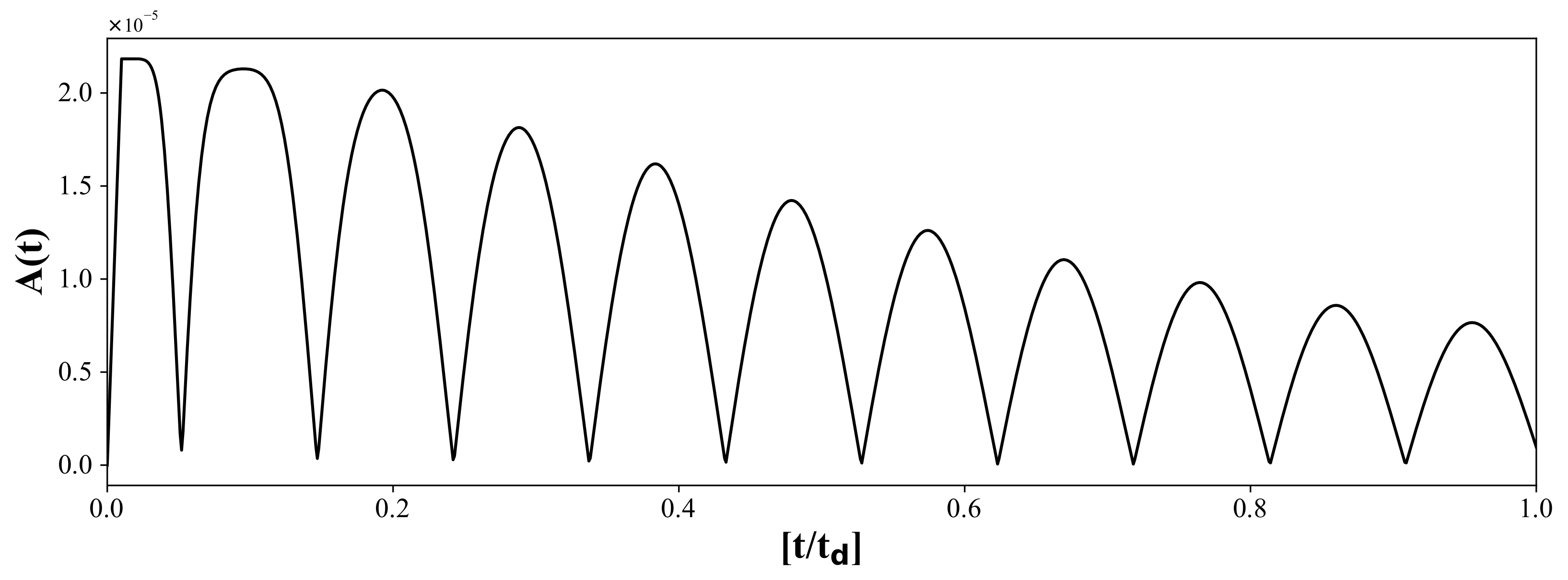
The inspection of the entropy production is evaluated by introducing the following functions:

$$S_1\left(t\right)=\frac{1}{\left[X\right]}{\int }_0^{\left[X\right]}\frac{f}{2}\left[U^2\left|U\right|\right]\left[\mathrm{d}x\right]$$

(78)

$$S_2\left(t\right)=\frac{1}{\left[X\right]}{\int }_0^{\left[X\right]}\frac{c_0{\eta }_{tur}}{p_0{L}_0}\left[\frac{1}{\rho }{\left(\frac{\partial U}{\partial x}\right)}^2\right]\left[\mathrm{d}x\right]$$

(79)

Figure 4 shows the evolution of both $S_1$ and $S_2$. Results reveal that the predominant role in the energy dissipation process is played by the compressibile turbulent effects.

In order to gain deeper insight into the phenomenon, the trend of spatially averaged of the ${\displaystyle \frac{p_0{L}_0}{c_0{\eta }_{tur}}}$ number:

$$N\left(t\right)=\frac{1}{\left[X\right]}{\int }_0^{\left[X\right]}\frac{p_0{L}_0}{c_0{\eta }_{tur}}\left[dx\right]$$

(80)

and of the $\left|{\displaystyle \frac{\partial U}{\partial x}}dt\right|$ number:

$$A\left(t\right)=\frac{1}{\left[X\right]}{\int }_0^{\left[X\right]}\left|\frac{\partial U}{\partial x}dt\right|\left[dx\right]$$

(81)

are computed. Results inspection reveals that $N\left(t\right)$ is almost constant ($N\left(t\right)\simeq$ 1.25 × 10${}^{-5}$); $A\left(t\right)$ is very close to zero, consistent with the ESM (Figure 5).

7. Conclusions

As an extension of previous works [14,17], we have examined the unsteady flow of a simple isotropic linear viscous fluid in the liquid state. We have suggested a new dimensionless procedure of the field equations. On the basis of the obtained results, we have conjectured that the transition from viscous to turbulent flow, which occurs when a finite amplitude pressure wave travels through the fluid, is governed by the dimensionless number ${\displaystyle \frac{p_0{L}_0}{c_0\eta }}$. This new dimensionless number is conceptually different from the Re number. The $Re$ number is related to the viscous forces arising from shape variation of the fluid particles, whilst the new dimensionless number is related to the viscous forces arising from volume variation; the $Re$ number governs the transition between the viscous and turbulent regimes during the fluid flow, whilst the new dimensionless number governs the transition which occurs when a pressure wave travels through the fluid. After some remarks on the role played by the elementary time scale in the closure equation for the turbulent bulk viscosity, we have applied the dimensionless procedure to the mean-flow equations which govern the unsteady turbulent flow regime, and we have identified a (second) new dimensionless number, given as ${\displaystyle \frac{p_0{L}_0}{c_0{\eta }_{tur}}}$. To test the performance of the dimensionless procedure, we have analyzed the experimental data concerning the 1D finite amplitude pressure waves propagation in liquid-filled pipe (water hammer phenomenon). We have shown that the experimental data roughly fall together on one curve. In line with the numerical simulation outcomes, this result is attributed to the reliability of the dimensionless procedure. The numerical results show good agreement with the experimental data. The analysis of the numerical results reveals the predominant role played by the ${\displaystyle \frac{p_0{L}_0}{c_0{\eta }_{tur}}}$ number in the turbulent compressible dissipation. Although we have suggested that the flow becomes unstable when the ${\displaystyle \frac{p_0{L}_0}{c_0\eta }}$ number exceeds its critical value, at the present there are no studies to support this conjecture, a critical value of the ${\displaystyle \frac{p_0{L}_0}{c_0\eta }}$ number is unknown, the details of the transition process are not available.

References

- Ghidaoui, M.S.; Zhao, M.; McInnis, D.A.; Axworthy, D.H. A Review of Water Hammer Theory and Practice. Appl. Mech. Rev. 2005, 58, 49–76. [Google Scholar] [CrossRef]
- Streeter, V.L.; Kestin, J. Handbook of fluid dynamics. J. Appl. Mech. 1961, 28, 640. [Google Scholar] [CrossRef] [Green Version]
- Duan, H.F.; Ghidaoui, M.S.; Lee, P.J.; Tung, Y.K. Relevance of unsteady friction to pipe size and length in pipe fluid transients. J. Hydraul. Eng. 2012, 138, 154–166. [Google Scholar] [CrossRef]
- Zielke, W. Frequency-Dependent Friction in Transient Pipe Flow. J. Basic Eng. 1968, 90, 109–115. [Google Scholar] [CrossRef]
- Trikha, A.K. An Efficient Method for Simulating Frequency-Dependent Friction in Transient Liquid Flow. J. Fluids Eng. 1975, 97, 97–105. [Google Scholar] [CrossRef]
- Pezzinga, G. Quasi-2D model for unsteady flow in pipe networks. J. Hydraul. Eng. 1999, 125, 676–685. [Google Scholar] [CrossRef]
- Zhou, J.; Bao, W.; Tick, G.R.; Moftakhari, H.; Cao, Q.; Ye, F. A weighting function model for unsteady open channel friction. J. Hydraul. Res. 2022, 60, 460–475. [Google Scholar] [CrossRef]
- Wahba, E. On the propagation and attenuation of turbulent fluid transients in circular pipes. J. Fluids Eng. 2016, 138, 031106. [Google Scholar] [CrossRef]
- Brunone, B.; Karney, B.W.; Mecarelli, M.; Ferrante, M. Velocity profiles and unsteady pipe friction in transient flow. J. Water Resour. Plan. Manag. 2000, 126, 236–244. [Google Scholar] [CrossRef] [Green Version]
- Wahba, E. Runge–Kutta time-stepping schemes with TVD central differencing for the water hammer equations. Int. J. Numer. Methods Fluids 2006, 52, 571–590. [Google Scholar] [CrossRef]
- Urbanowicz, K.; Bergant, A.; Karadžić, U.; Jing, H.; Kodura, A. Numerical investigation of the cavitating flow for constant water hammer number. J. Phys. Conf. Ser. 2021, 1736, 012040. [Google Scholar] [CrossRef]
- Durst, F. Fluid Mechanics: An Introduction to the Theory of Fluid Flows; Springer Science & Business Media: New York, NY, USA, 2008. [Google Scholar]
- Jou, D.; Casas-Vazquez, J.; Lebon, G. Extended irreversible thermodynamics revisited (1988–98). Rep. Prog. Phys. 1999, 62, 1035. [Google Scholar] [CrossRef]
- Di Nucci, C.; Pasquali, D.; Celli, D.; Pasculli, A.; Fischione, P.; Di Risio, M. Turbulent bulk viscosity. Eur. J. Mech.-B/Fluids 2020, 84, 446–454. [Google Scholar] [CrossRef]
- Di Nucci, C.; Petrilli, M.; Russo Spena, A. Unsteady friction and visco-elasticity in pipe fluid transients. J. Hydraul. Res. 2011, 49, 398–401. [Google Scholar] [CrossRef]
- Di Nucci, C.; Russo Spena, A. On the propagation of one-dimensional acoustic waves in liquids. Meccanica 2013, 48, 15–21. [Google Scholar] [CrossRef]
- Di Nucci, C.; Russo Spena, A. On transient liquid flow. Meccanica 2016, 51, 2135–2143. [Google Scholar] [CrossRef]
- Di Nucci, C.; Celli, D.; Fischione, P.; Pasquali, D. Elementary scales and the lack of Fourier paradox for Fourier fluids. Meccanica 2022, 57, 251–254. [Google Scholar] [CrossRef]
- Landau, L.D.; Lifshitz, E.M. Fluid Mechanics (Course of Theoretical Physics, Volume 6); Elsevier: Amsterdam, The Netherlands, 2013. [Google Scholar]
- Di Nucci, C.; Celli, D. From Darcy Equation to Darcy Paradox. Fluids 2022, 7, 120. [Google Scholar] [CrossRef]
- Gad-el Hak, M. The fluid mechanics of microdevices—The Freeman scholar lecture. J. Fluids Eng. 1999, 121. [Google Scholar] [CrossRef]
- Panton, R.L. Incompressible Flow; John Wiley & Sons: Hoboken, NJ, USA, 2005. [Google Scholar]
- Meniconi, S.; Brunone, B.; Ferrante, M.; Massari, C. Transient hydrodynamics of in-line valves in viscoelastic pressurized pipes: Long-period analysis. Exp. Fluids 2012, 53, 265–275. [Google Scholar] [CrossRef]
- Comsol AB. COMSOL Multiphysics™; Comsol AB: Stockholm, Sweden, 2016. [Google Scholar]
Figure 1.
Experimental data [23].
Figure 2.
Experimental data scaled according to , m/s, = 350 m/s, = D = 93.5 mm.
Figure 3.
Comparison between experimental and numerical results, for .
Figure 4.
Temporal variation of and , for = 33,588.
Figure 5.
Temporal variation of , for = 33,588.