
Tsunami-Induced Bore Propagating over a Canal—Part 1: Laboratory Experiments and Numerical Validation


1
Department of Civil Engineering, University of Ottawa, Ottawa, ON K1N 6N5, Canada
2
Department of Civil Engineering, Lakehead University, Thunder Bay, ON P7B 5E1, Canada
*
Author to whom correspondence should be addressed.
Fluids 2022, 7(7), 213; https://0-doi-org.brum.beds.ac.uk/10.3390/fluids7070213
Submission received: 13 May 2022
/
Revised: 12 June 2022
/
Accepted: 20 June 2022
/
Published: 22 June 2022
Abstract
:This companion paper investigates the hydrodynamics of turbulent bores that propagate on a horizontal plane and have a striking resemblance to dam break waves and tsunami-like hydraulic bores. The focus of this paper is on the propagation of a turbulent bore over a mitigation canal using both laboratory experiments and numerical simulations. In the first part of this paper, the effects of canal depth on the time histories of wave height and velocity were experimentally investigated, and the experimental results were used for the validation of the numerical model. The rapid release of water from an impoundment reservoir at depths of do = 0.30 m and 0.40 m generated bores analogous to tsunami-induced inundations. The time histories of the wave heights and velocities were measured at 0.2 m upstream and at 0.2 m and 0.58 m downstream of the canal to study the energy dissipation effect of the mitigation canal. The recorded time series of the water surface levels and velocities were compared with simulation outputs, and good agreement was found between the experimental and numerical water surface profiles, with a Root Mean Square Error (RMSE) of less than 6.7% and a relative error of less than 8.4%. Three turbulence models, including the standard k-ε, Realizable k-ε, and RNG k-ε, were tested, and it was found that all these models performed well, with the standard k-ε model providing the highest accuracy. The velocity contour plots of the mitigation canal with different depths showed jet streams of different sizes in the shallow, medium-depth, and deep canals. The energy dissipation and air bubble entrainment of the bore as it plunged downward into the canal increased as the canal depth increased, and the jet stream of the maximum bore velocity decreased as the canal depth increased. It was found that the eye of the vortex created by the bore in the canal moved in the downstream direction and plunged downward in the middle of the canal, where it then began to separate into two smaller vortices.
1. Introduction
Tsunami-induced bores are infrequent but are extremely destructive and can cause significant infrastructure damage in coastal regions. The most common source of tsunami waves are earthquakes, ones either near or beneath the ocean, and the resulting tsunami bores can become massive far from their points of origin [1]. Despite the availability of new design guidelines for coastal structures, post-tsunami field investigations of past events have revealed that many nearshore structures were completely destroyed or significantly damaged during these events [2,3,4]. The recent tsunami events in the Indian Ocean in 2004, in Japan in 2011, and in Indonesia in 2018 showed the destructive energy of tsunami-induced loads. As a result, more safety measures and design guidance should be considered in order to minimize human casualties and ensure safe critical infrastructure in coastal areas [5]. Field observations of tsunami waves have indicated that return wave periods range from 10 min to 45 min [6]. In deep water and far from the shore, tsunami waves can reach velocities of the order of hundreds of kilometers/hour and can propagate toward the shoreline without a substantial loss in their kinetic energy. Once a tsunami wave approaches the coastal region, its velocity decreases, its height increases, while their wave period remains constant. Depending on the tsunami wave characteristics and the nearshore bathymetry, the wave’s leading edge can break to form a turbulent bore or a bore even right before the wave reaches the shoreline [7,8].
An analysis of video images of the tsunami waves which propagated overland in several coastal regions of the Indian Ocean in 2004 showed a strong similarity between dam-break waves propagating on a horizontal plane and tsunami-like hydraulic bores [9]. As a result, researchers started employing dam-break waves to model tsunami inundation in laboratory studies [3,10,11,12,13,14,15,16,17,18,19,20,21,22]. Various water-release mechanisms have been used to generate dam-break bores. A volume of water stored in a reservoir could be released by a rapidly opening swing gate [23,24], by the sudden removal of a vertical gate [25,26,27,28], or by releasing an elevated volume of water through vertical pipes [12,13,29,30,31]. In order to model tsunami wave inundations, several experiments generated dam-break waves by rapidly releasing water impounded from behind a vertical gate [7,8,10,15,16,24,32,33]. The differences between hydraulic bores flowing over dry beds and those flowing over stagnant water, known as a wet bed, have been examined using laboratory experiments and numerical simulations [10,34,35]. For the same initial impoundment depth, a bore propagating over a wet bed is higher, and its wave front is steeper in comparison to that of a bore with an equivalent initial wave height propagating over a dry bed [12]. Additionally, the velocity of a bore front propagating over a wet bed is affected by the still water depth. Hydraulic bores from impoundments of the same depth have higher velocities when propagating over the shallower still water depths [7].
The influences of tsunami mitigation structures on tsunami wave energy dissipation have been investigated in the past by studying the characteristics of wave hydrodynamics before and after different natural and manmade obstacles such as pine forests [36], coastal dunes [37], rivers and canals [38,39], and natural and artificial buildings [40]. During bore propagation over natural streams or manmade canals, the upstream water level increases while the bore velocity decreases due to energy dissipation within the canal. Figure 1 shows an aerial image of the 2011 Japan Tsunami propagating over a canal running parallel to the coastline.
Laboratory experiments have shown that the hydrodynamic features of tsunami waves are considerably changed during their propagation over natural streams. Ref. [41] showed how the destructive energy of tsunami waves was dissipated over a mitigation canal by conducting tests at three impoundment water depths of do = 0.55 m, 0.79 m, and 0.80 m. Only one canal geometry was tested, with a width of w = 0.30 m and a depth of d = 0.05 m, which gives a canal aspect ratio of w/d = 6. The overflow wave velocity was shown to have been reduced by the canal, while the wave height downstream of the canal increased. Ref. [42] indicated that the maximum reduction in wave velocity downstream of a canal occurred for the deepest and widest canals. A narrow range of canal aspect ratios of w/d = 4 to 10 was used. The physical experiments showed a similar wave velocity reduction when the canals had different depths but the same width. However, delays in the tsunami propagation were observed, and velocity mitigation occurred for all canal configurations. It was observed that the tsunami wave energy can be partially absorbed by the reflected wave generated by the canal. Recently, a series of laboratory experiments was conducted to examine the effects of canal geometry on the hydrodynamics of turbulent bores passing over a rectangular mitigation canal installed perpendicular to the flow direction [39]. The surface water level and wave velocity were measured both upstream and downstream of the canal, and the effect of canal geometry was tested for a wide range of canal aspect ratios (i.e., 4 ≤ w/d ≤ 60) in order to study the variations in wave heights and velocities for canal optimization.
Tsunami-like bores have been numerically simulated to provide more insight into the wave hydrodynamics and energy transfers during wave propagation and impact with coastal structures. Ref. [10] performed numerical simulations of tsunami-like bores with an upstream water depth of do = 0.85 m with the use of a structural model. A discrepancy was found in the early stages of the bore–structure interaction due to the significant splashing of water at the initial impact, which was not accurately reproduced by the numerical model. However, relatively good agreement was achieved between the numerical results and measurements after approximately 3 s of the bore initiation. Ref. [43] investigated the effect of still water depth on the hydrodynamics of tsunami waves and wave structure interactions using a 3D Smoothed Particle Hydrodynamics (SPH) model. The time series of the net total base horizontal force acting on a slender square column were modelled, and it was found that the hydrodynamic loads due to hydraulic bore propagation were greatly correlated with still water depth. Ref. [44] performed a comparison of experimental and computational time series of water surface profiles for a dam-break wave with an upstream water depth of do = 0.85 m; they found that the initial run-up tongue reached its peak elevation at t = 1.9 s, and that it collapsed under the effect of gravity. In [11], the time variations of bores’ water surface profiles passing over a triangular obstacle were simulated using the OpenFoam software package, and the numerical results were compared with measurements. The results of the numerical simulation using the standard k-ε turbulence model agreed well with the experimental results, but the time series of the water surface downstream of the triangular obstacle was not in good agreement with the measurements.
The main objective of the present companion paper is to evaluate the performance of a three-dimensional transient Computational Fluid Dynamics (CFD) model [45] in simulating the propagation of a turbulent bore over a mitigation canal. The paper aims to evaluate the capability of the proposed numerical model to simulate such complex turbulent and transient flows and to select the most suitable turbulence model for accurate simulations. Model evaluation was achieved by comparing the time histories of water surface elevations and bore velocities, and the performance of three turbulence models was tested. After model validation, the numerical outputs were further analyzed to investigate the effect of canal depth on the wave characteristics and to understand the mitigation effects of a rectangular canal by comparing water surface elevations and velocities before and after the canal. The effects of the mitigation canal on variations in specific momentum and energy dissipation are studied in the second part of this companion paper. As shown in Figure 1, the tsunami wave propagated over a manmade canal with different angles of incidence against the tsunami wave. The effects of canal inclination on the energy dissipation of hydraulic bores are also presented in the second part of this companion paper.
2. Experimental Set-Up
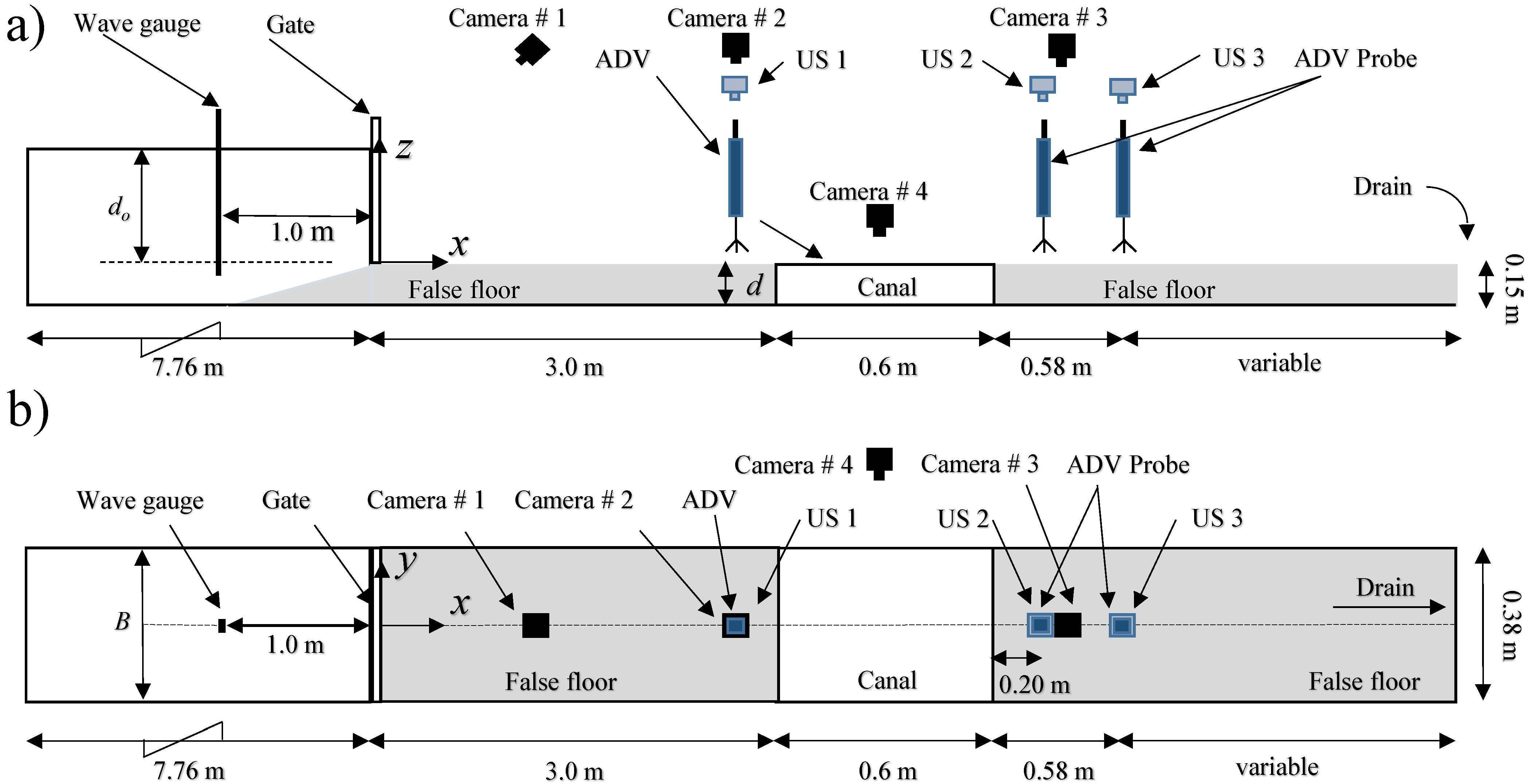
Laboratory experiments were conducted in the Water Resources Laboratory at the University of Ottawa, Canada. A glass-walled tilting flume that was 15.56 m long, 0.38 m wide, and 0.60 m deep was used to perform the laboratory experiments. The schematic of the experimental setup and the coordinate system is shown in Figure 2. A false floor was made of several parallelepipeds (PVC, Canus Plastics Inc., Ottawa, ON, Canada) of different sizes to form a rectangular canal with varying depths and widths. Two impoundment depths of do = 0.3 m and 0.4 m were set by installing a vertical gate (Plexiglas, Canus Plastics Inc., Ottawa, ON, Canada) located at 7.76 m downstream of the flume reservoir (see Figure 3a). The vertical gate was firmly fixed at the upstream end of the false floor such that water leakage would be minimized. The released impounded water generated a turbulent bore which propagated over the smooth horizontal bed. The generated bore interacted with the rectangular mitigation canal, which then continued to propagate to the end of the flume and then, through a drain, into the downstream reservoir. The canal width was constant (w = 0.60 m), and three depths of d = 0.05 m, 0.10 m, and 0.15 m were examined (see Table 1).
Four wireless video cameras (GoPro, Hero5, SanMateo, CA, USA) were used to monitor the propagation of the bore front and the bore wave passing over the canal. The first camera was positioned on the side of the flume at the lengthwise half-way point of the canal in order to visualize the bore front and capture the bore profiles. The other three video cameras were positioned on top of the flume at different locations between the gate and the upstream end of the canal in order to monitor the motion of the bore front. A 1V:6H ramp (PVC, Canus Plastics Inc., Ottawa, ON, Canada) was installed at the upstream end of the false floor to reduce flow separation and local energy losses before the mitigation canal. The mitigation canal was located at 3.0 m downstream of the gate to ensure the formation of a fully developed hydraulic bore. The false floor was marked on the bed with parallel tape lines with a 0.05 m distance between each other (see Figure 3). The marked bed was used to measure the bore front velocity using a high-speed image-tracking technique (particle tracking velocity-based). Plastic beads with a diameter of 0.015 m were placed on the flume bed downstream of the gate. They moved as the lift gate was opened, and a GoPro camera with a shutter speed of 60 frames per second was positioned above the marked section to capture the propagation of the beads over a marked 0.60 m long section. The bore frontal velocity was measured by computing the travel distance of the beads between two adjacent parallel lines in two consecutive images.
The volumes of water in the reservoir for the impoundment depths of do = 0.4 m and 0.3 m were 1.62 m3 and 1.21 m3, respectively. The equivalent aspect ratios of reservoir L/do for do = 0.4 m and 0.3 m were 26.61 and 35.47, respectively, both of which were considerably larger than the minimum reservoir aspect ratio (i.e., L/do = 11.05) suggested by [32]. To generate a fully developed dam-break wave, the lifting speed of the vertical gate was measured by a high-speed camera and compared with the maximum opening time. Ref. [32] indicated that a dam-break wave would develop fully if the non-dimensional gate-opening time To = to(g/do)1/2 was less than 21/2, where to is the gate-opening time. Theoretically, the time required to open the gate is the time it takes for the topmost water particles to fall in order to produce a dynamic wave followed by a horizontal translational motion. In this study, the time to open the gate was monitored with a high-speed camera, and the measured non-dimensional gate-opening times were in the range of 0.70 < To < 0.825.
Two wave gauge sensors were used to measure the time histories of the water surface levels. A capacitance-type wave gauge (model WG-50, manufactured by RBR Ottawa, ON, Canada) was used to measure the time history of the water level in the reservoir, with a sampling frequency of 1200 Hz. This capacitance-type wave gauge sensor was mounted 1 m upstream of the gate and was labeled as WG (see Figure 3a). Three ultrasonic wave gauge sensors (MASSA, M-5000/220, Hingham, MA, USA) were deployed upstream and downstream of the canal to measure the time series of the water surface, with a sampling frequency of 1200 Hz (see Figure 3b). An acoustic Doppler velocimeter (ADV) probe (Nortek-AS, Vangkroken, Rud, Norway) was used to measure the time histories of the velocity, with a sampling frequency of 200 Hz. The ADV probe measured the instantaneous velocity at z = 0.01 m above the surface of the false bed. The ultrasonic wave sensors were labelled as US, and the velocity sensors were labelled as ADV. Both the water surface levels and velocities were measured at the centerline of the flume and at 0.2 m upstream (US1/ADV1) and at 0.2 m (US2/ADV2) and 0.58 m (US3/ADV3) downstream of the canal (see Figure 3b). All the experimental runs were repeated three times to ensure the repeatability of the tests and to obtain averaged time-series data from the sensors.
3. Numerical Simulation
A two-phase (i.e., water and air), three-dimensional numerical model (OpenFOAM) v5.0 was used for the numerical simulations. Three types of turbulence models were analyzed in order to identify the most accurate numerical results. The open-source feature of OpenFOAM enables users to modify and expand the functionality of the solver package according to the requirements of their specific project. The Finite Volume Method (FVM) was used to model the hydraulic bore propagation over a smooth horizontal bed, and the InterFoam solver was used to solve the continuity, momentum (i.e., Navier-Stokes), and turbulence equations. The time-averaged form of the Navier–Stokes equations, known as the Reynolds-Averaged Navier–Stokes (RANS), was used in this study, and the turbulence closure equation was the well-known k-ε model with different modifications. The performances of the classic k-ε, Realizable k-ε, and Renormalization Group (RNG) k-ε turbulence models were examined to be able to select the most accurate numerical results.
The continuity equation in a cubic control volume was solved at each time step, and mass conservation was achieved by setting the net flow in the cubic control volume as [46]:
where , , and are the components of the mean velocity in the x, y, and z directions, respectively. The instantaneous velocities were decomposed to the mean flow and velocity fluctuations as [46]:
Where , and are the velocity fluctuations in the x, y, and z directions, respectively. The momentum equation for a three-dimensional domain, known as a Navier–Stokes equation, can be expressed as follows [46,47]:
where t is the time, p is the fluid pressure, g is the gravitational acceleration, and ρ is the fluid density. A phase fraction equation is required to model the spatial distribution of two different fluids (i.e., air and water) at any particular time step. The phase fraction α is a scalar quantity, which is one for water and zero for air. The value of the phase fraction determines the transitional region. The phase fraction α parameter is a conserved quantity and can be described by the transport equation as follows [48]:
where is the divergence, and is the velocity vector. The density of the air–water mixture in the water surface cells can be calculated as [48]:
The Navier–Stokes equations can predict the motion of a fluid. Regarding the technique that the user needs to deal with turbulent fluctuations in the flow, OpenFOAM provides various techniques. These equations are stated in Cartesian coordinates and tensor notation while disregarding body forces. Thus, the RANS conservation equations of the mass and momentum of an incompressible fluid are shown in [49]. It is impossible to answer the momentum and continuity equations analytically, except for a very few straightforward conditions. To close the equations, a novel idea of turbulent viscosity was developed by Boussinesq, and the Reynolds stresses can be numerically defined by time-averaging the flow equations [49].
All the parameters inside the flume domain (except for the canal and the reservoir), such as water depth, phase fraction, pressure, velocity, and force, had an initial value of zero. The phase fractions for the canal and the reservoir were equal to 1, indicating that those domains were filled with water. Figure 4a shows the computational domain for the water surface profile upstream of the gate and inside the canal. The simulated flume dimensions and water level at the beginning of the test at t = 0 are also shown in this figure. The length of the upstream reservoir is exactly half of the overall flume length. The desired upstream impoundment depth and the amount of water in the canal were established by setting a different initial phase fraction than for the rest of the flume. Figure 4b,c show the mesh resolution in the upstream reservoir and in the canal. The mesh size for all directions was set to 10 mm, and the number of mesh layers was controlled by the impoundment and canal depths. Figure 4d,e display the three-dimensional water surface profiles of the turbulent bore front and its interaction with the canal at t⁎ = 0.25 s and 0.50 s after the bore front plunged into the canal; t⁎= 0 is when the bore reaches the upstream edge of the canal. At t⁎ = 0.25 s, a deep plunge and water surface rolling were observed as a result of a heavy shear layer formation. A surface jump started to occur at t⁎ = 0.50 s, and then, over time, the water depth in the canal increased.
All boundary conditions were set as “wall boundary with no-slip”, except for the wall located downstream of the flume, on which an “outlet with a zero gradient” was imposed. This latter outlet boundary condition permitted water to exit from the computational domain. A systematic mesh independence analysis was performed, similar to those in the studies by [50,51]. A comparison of the numerical outcomes using different mesh resolutions indicated that a domain with a cell size of 10 mm × 10 mm × 10 mm replicated the experimental results with a reasonable accuracy, with a root mean square error (RMSE) of less than 6.7% and a relative error of less than 8.4%.
4. Results and Discussion
4.1. Model Validation
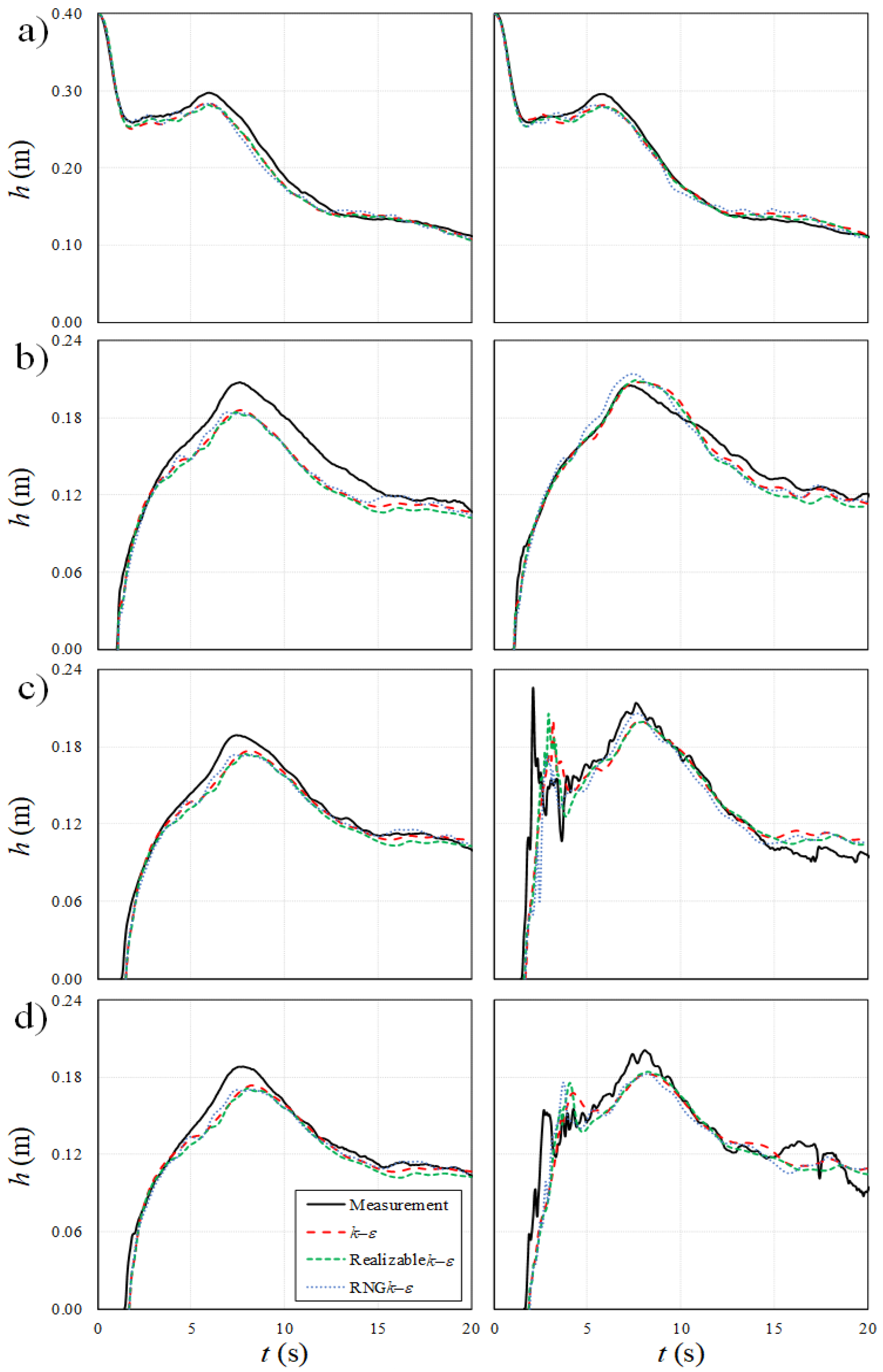
The time histories of the water surface levels and velocities at four locations: 1.0 m upstream of the gate, 0.2 m upstream of the canal, and 0.2 m and 0.58 m downstream of the canal, were extracted from the numerical models, and the results were compared with the measurements. Model validations were performed in both the absence and presence of a rectangular canal and for an impoundment depth of do = 0.4 m. The canal dimensions for model validation were w = 0.6 m and d = 0.15 m. Figure 5 shows the comparison of the simulated time histories of water surface profiles with the experimental results. The subplots in the left column show the time histories of the water depth in the absence of a canal, while the subplots in the right column show the same variables in the presence of a rectangular canal. Sensitivity analyses have been conducted in previous studies to select a proper turbulence model [11,15,16,33], and in order to improve simulation accuracy, three k-ε-based turbulence models (i.e., classic k-ε, Realizable k-ε, and RNG k-ε) were implemented.
Figure 5a shows the performance of the numerical model at 1.0 m upstream of the gate; the numerical results were compared with the measurements from the capacitance-type wave gauge (WG). As it can be seen, the turbulent bore height peaked and then gradually decreased over time. For the water surface profiles of the bore propagating over the horizontal surface, the maximum simulated water level was approximately 4% less than the measured peak water depth. The experimental and numerical results for the maximum bore heights measured at 1.0 m upstream of the gate and without a canal were 0.30 m and 0.28 m, respectively. The peak water levels occurred at approximately the same time (i.e., t = 5.9 s) for both laboratory experiments and numerical simulations. For the water surface profiles when propagating over the canal, the peak water elevation was about 5% smaller than the measured peak water depth. The experimental and numerical results for the maximum bore heights at 1.0 m upstream of the gate and in presence of a canal were 0.30 m and 0.28 m, respectively. For the water surface profiles over the horizontal bed, a small discrepancy was found between the experimental and numerical results for 5 s ≤ t < 13 s. For 13 s ≤ t < 17 s, the bore became almost similar to a quasi-steady flow. The bore height linearly decreased with time for the water surface profiles over a horizontal surface and over the rectangular canal for t ≥ 17 s. The results revealed that all three turbulence models were able to simulate the experiments at the position of the WG.
The time series of water surface profiles at 0.2 m upstream of the canal (US1) are shown in Figure 5b. As it can be seen, in the absence of a canal, the maximum simulated water surface profile was approximately 10% lower than that measured. The water surface profile rose steadily from zero, reached its peak, and then declined over time. The maximum measured and simulated water levels at this location were 0.21 m and 0.19 m, respectively. In the presence of the canal, the measured and simulated peak water depths were the same, with a value of 0.21 m. The times to reach the peak water depth in the absence and presence of a canal were 7.7 s and 7.8 s, respectively. For t ≥ 15 s, the water surface profiles in the absence and presence of a rectangular canal became similar to a quasi-steady state profile. At this location, the three turbulence models provided approximately the same water surface profiles.
Figure 5c displays the temporal variations in the water surface levels at 0.2 m downstream of the canal (US2). The maximum simulated water depths for both cases with and without a canal were 6% smaller than those measured. The maximum experimental and numerical water depths in the absence of a canal were 0.19 m and 0.18 m, respectively. However, in the presence of a canal, the water depths were 0.21 m and 0.20 m, respectively. In addition, the times to reach the peak water depth without and with the canal were t = 8.0 s and 7.8 s, respectively. The slight difference in the simulations of peak water depth after the canal may be attributed to air entrainment and bubble formation in the canal. The entrained bubbles were formed by the bore plunging into the canal. The time histories of the bore height at 0.58 m downstream of the gate (US3) are shown in Figure 5d. It was observed that the simulated water surfaces in the absence of a canal were 7% smaller than those measured, but the times to reach the peak were similar, with a value of t = 8.2 s. In the presence of the canal, the simulated peak water depth was 9% smaller than that measured. The performance of the standard k-ε model in reproducing this element was slightly better than that of the other turbulence models (see Table 2).
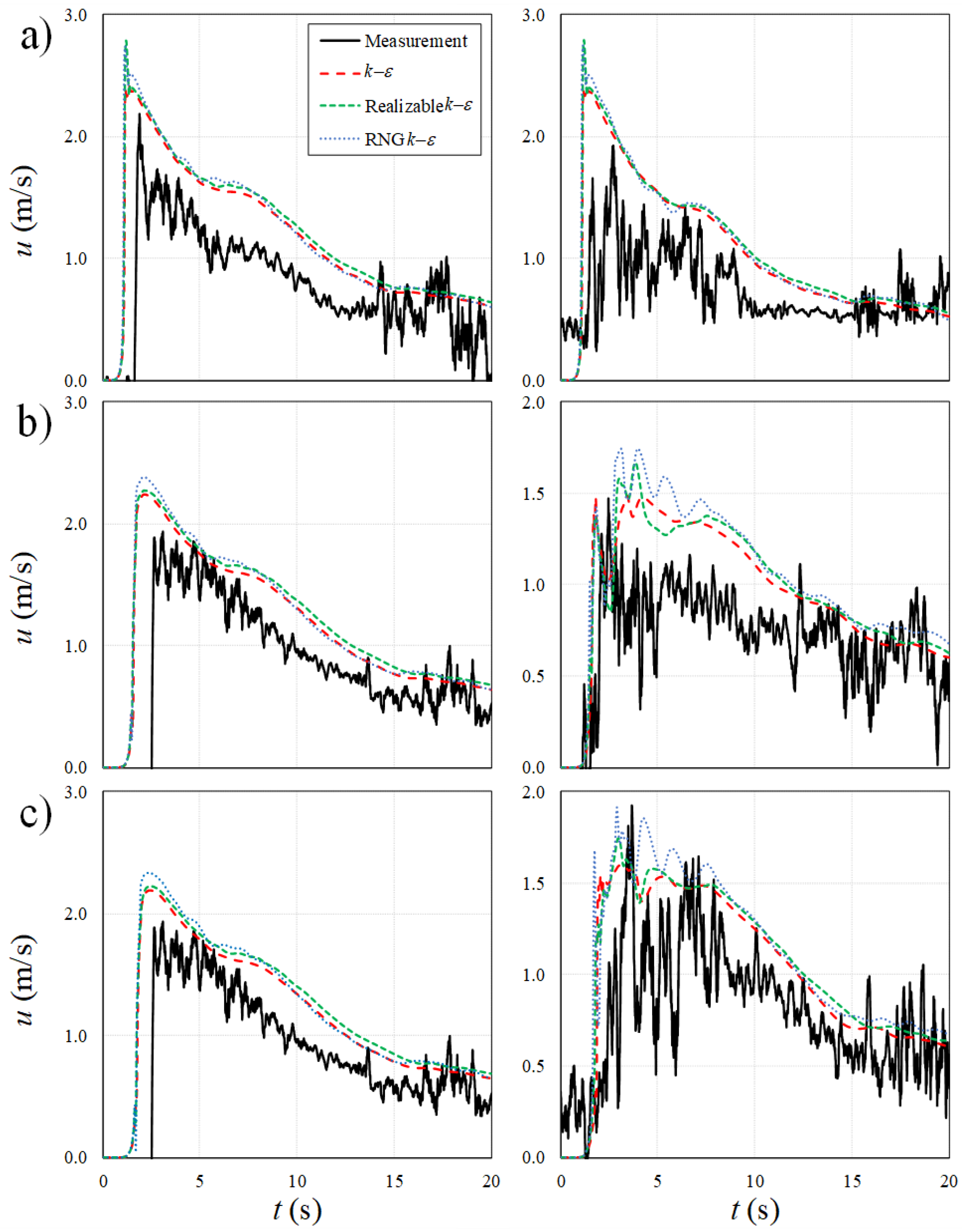
The time series of the water velocities of the bore generated by an impoundment depth of do = 0.4 m were extracted from the numerical model results for both the absence and presence of the rectangular canal (w = 0.6 m, d = 0.15 m). The simulated bore velocity profiles were compared with measurements at three different positions: ADV1, ADV2, and ADV3 (see Figure 6). Comparison of the numerical outcomes with the measurements indicated that the simulated time histories of the water velocities were overestimated compared to the measurements. As shown in Figure 6, the bore front in the horizontal bed tests reached the canal earlier than the front identified by the measurements, whereas in the presence of a canal, the simulated bore front velocities were similar to those from the measurements.
Figure 6a shows the time histories of the bore velocities in the absence and in the presence of a canal at 0.20 m upstream of the canal (ADV1). For the bore velocity profiles over a horizontal bed without a canal, the maximum measured peak bore velocity was approximately 9.5% lower than the simulated peak bore velocity. The measured and simulated peak bore velocities in the horizontal bed tests were 2.19 m/s and 2.42 m/s, respectively. For the bore velocity profiles over a canal, the maximum measured bore velocity was approximately 20% less than that from the simulation results. The measured and simulated bore velocities in the presence of a canal were 1.93 m/s and 2.41 m/s, respectively. Figure 6b shows the temporal variations of the bore velocity profiles at 0.20 m downstream of the canal (ADV2). In the absence of a canal, the peak measured bore velocity was 11% smaller than the simulated ones; however, the maximum measured and simulated bore velocities were approximately the same over the canal surface. In the absence of a canal, the experimental and numerical bore velocities at 0.20 m downstream of the canal (ADV2) were 1.99 m/s and 2.24 m/s, respectively. In the presence of a canal, the experimental and numerical bore velocities were 1.47 m/s and 1.49 m/s, respectively.
The time series of the bore velocities at 0.58 m downstream of the canal (ADV3) are shown in Figure 6c. It was observed that the maximum measured bore velocity in the absence of a canal was lower than the simulated velocity by 11.5%, with values of 2.19 m/s and 1.94 m/s, respectively. In contrast, in the presence of a canal, the maximum measured bore velocity was higher than the simulated peak velocity by 17%, with values of 1.92 m/s and 1.60 m/s, respectively. However, the inaccuracy in predicting the commencement of the bore and the maximum bore velocity still appeared in the horizontal bed tests, as shown in Figure 6b,c (see Table 2).
The underestimation of the velocity measurements obtained with the ADV probe is due to the fact that ADV data tend to be affected by the high turbulence. The high turbulence can occasionally generate cavitation around the tip of the AVD, which induces unwanted noise in the signal, thus influencing the results. The effect of the high turbulence on the ADV recording can be observed indirectly since the time histories of the experimentally measured and the calculated bore velocities are almost the same after about 15 s, when flow turbulence reduces significantly. Overall, the accuracy of the time histories of the measured bore velocity results is highly dependent on the precision of the ADV probe.
4.2. Water Surface Variations with Time
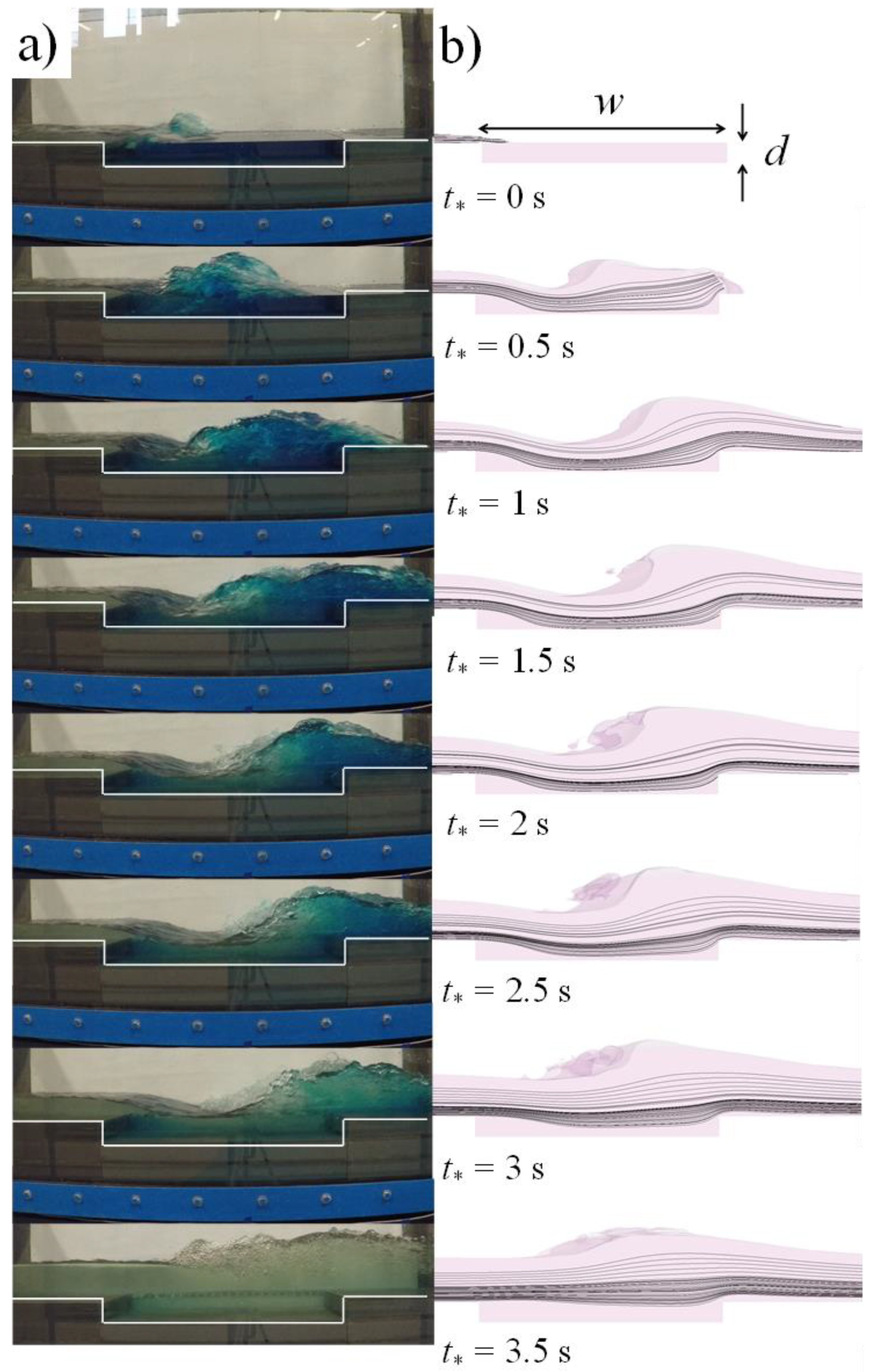
Figure 7a shows a series of consecutive images of water surface profiles as the bore propagates over a canal with a depth of d = 0.05 m.
Blue dye was added to the stationary water in the canal for a better visualization of the bore arrival and mixing. Once the bore front reached the upstream edge of the canal, a sequence of ripples formed on the surface of the bore as it travelled over the canal. At t⁎ = 0.50 s, the bore front plunged into the canal and initiated a surface hydraulic jump. The bore height was amplified due to a substantial increase, and a surface hydraulic jump formed in the middle of the canal. After a short period of time, at t⁎ = 1.0 s, the bore height increased again and reached the downstream edge of the canal. At t⁎ = 1.5 s, the bore front expended some of its momentum into the stagnant water in the canal, displacing the water in the canal and causing it to peak. A strong shear layer formed due to the existence of a quasi-steady flow in the upstream of the canal, and as a result, a strong surface jump formed at the downstream end of the canal, at 2 s ≤ t⁎ ≤ 2.5 s. At this stage, the water surface level increased with time and reached its maximum value at 3 s ≤ t⁎ ≤ 3.5 s. For t⁎ > 3.5 s, a rapid change in the water surface profile occurred, flattening the water surface profile.
This bore–canal interaction suppressed the energy of the bore. As such, one could use such canals to protect coastal or near-shore infrastructure against tsunami inundation hazards. The simulated three-dimensional water surface profiles and streamlines observed when the bore passed over the canal were extracted from validated numerical models. Figure 7b shows consecutive images of the simulated water surface profiles, starting from t⁎ = 0 s and with a time interval of 0.5 s. A comparison of the experimental water surface profiles obtained from video images and those from the numerical simulations indicated very good agreement. At t⁎ = 0 s, the simulated water surface profile and streamlines reached the upstream edge of the canal. At t⁎ = 0.5 s, the measured bore front reached the downstream edge of the canal, whereas the simulated streamlines reached the canal bottom at a distance of approximately 0.17 m from the upstream edge of the canal. At t⁎ = 1.0 s, the bore propagated further downstream of the canal, but no change was observed in the spreading of the simulated bore front. The measured and simulated bores showed a similar trend in water surface level for 1.5 s ≤ t⁎ ≤ 2.0 s. The simulated turbulent bores continuously affected the volume of water observed in the sector of the canal for 0.5 s ≤ t⁎ ≤ 3.5 s.
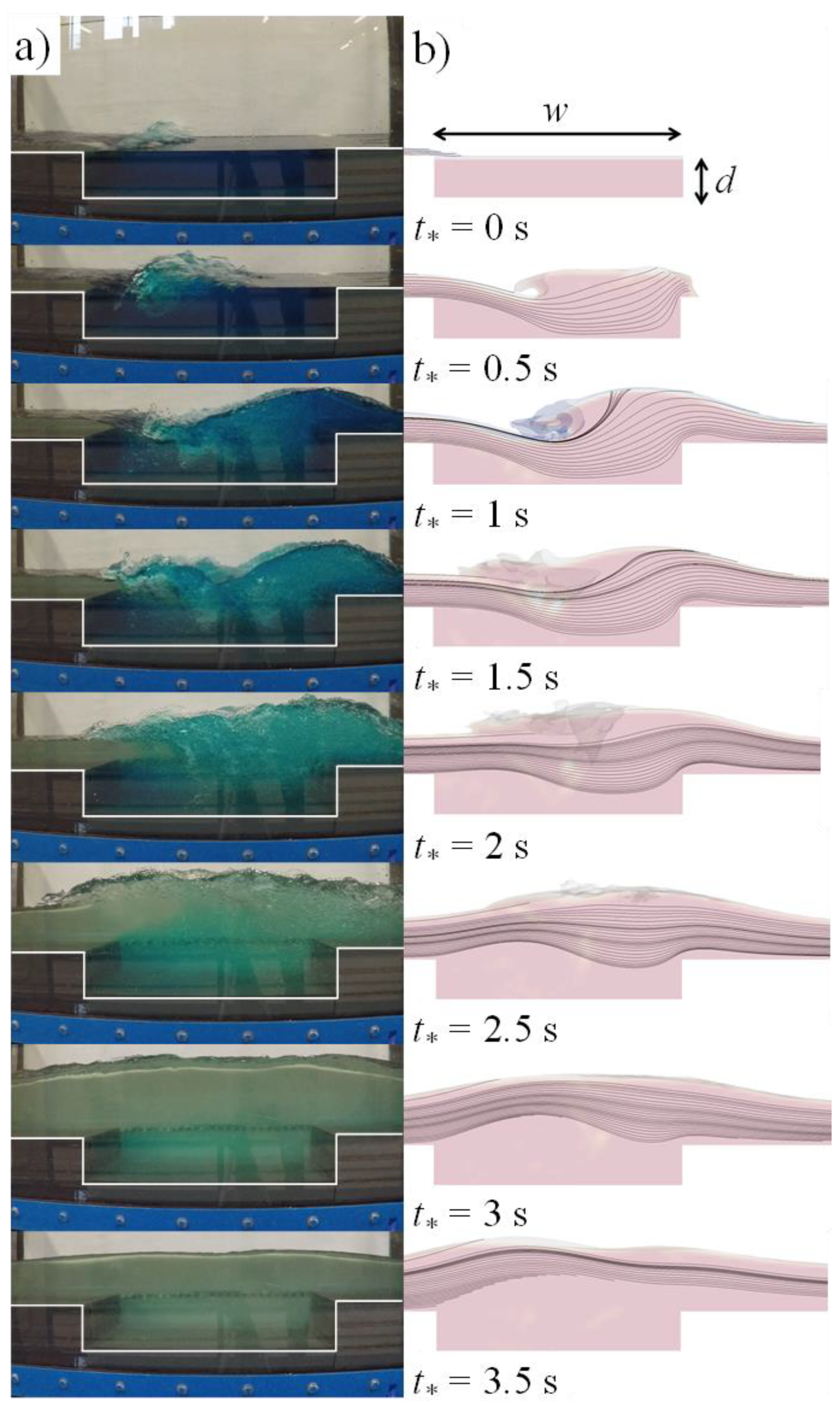
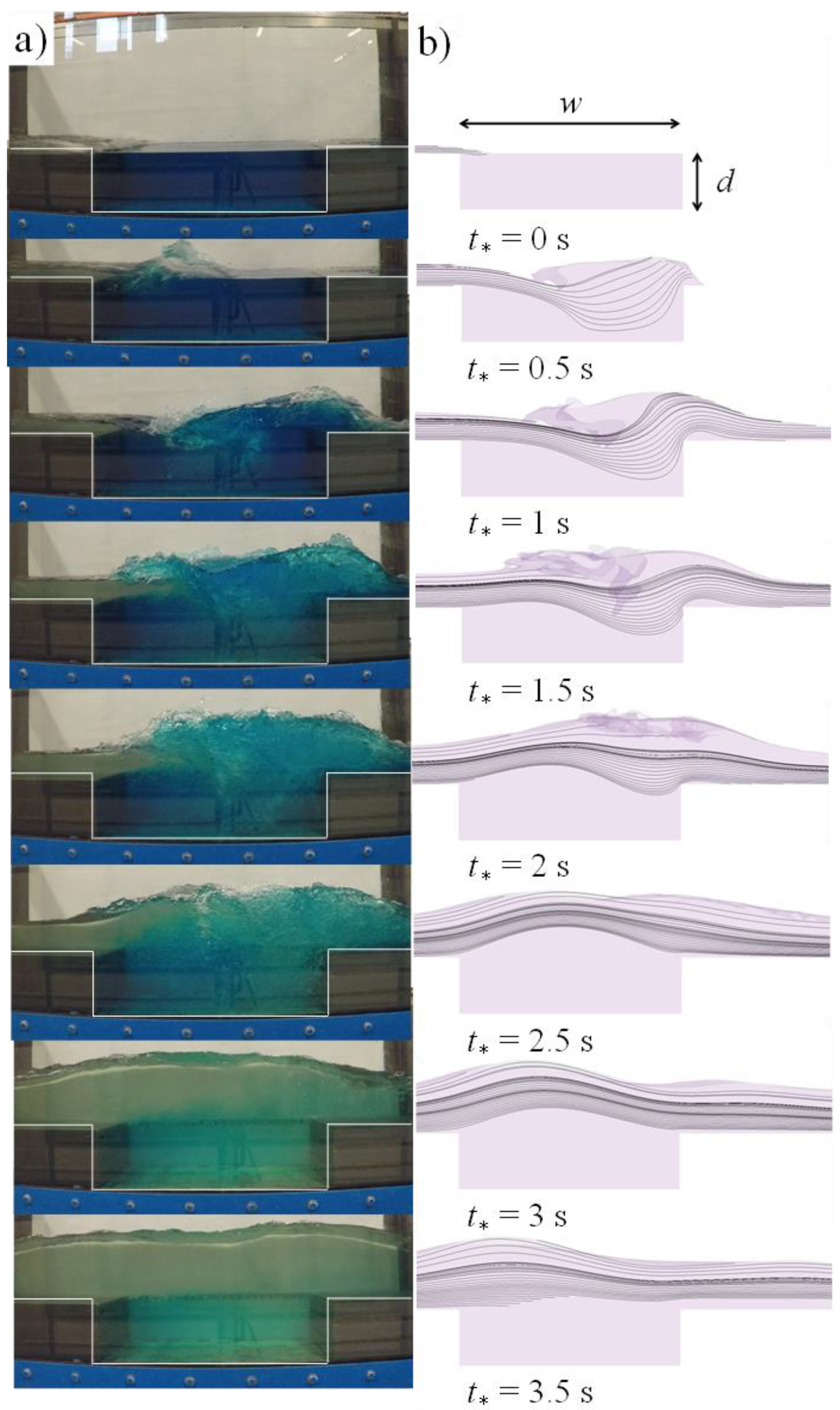
Analogous to simulations of a hydraulic bore passing over a shallow canal with a depth of d = 0.05 m, the time histories of the water surface profiles and flow streamlines passing over medium-depth and deep canals with depths of d = 0.10 m and d = 0.15 m, respectively, are shown in Figure 8 and Figure 9. As can be seen in Figure 8, the simulated turbulent bore passing over a medium-depth canal with a depth of d = 0.10 m reached the canal end at t⁎ = 0.5 s, while the toe of the surface jump was located at approximately 0.28 m from the upstream edge of the canal. At the bottom of the canal, the simulated streamlines slowly rose at time at t⁎ = 1.0 s. The time histories of the water surface profiles and streamlines passing over the deep canal with a depth of d = 0.15 m are shown in Figure 9. These simulated streamlines did not reach the bottom of the canal during the passage of the turbulent bore. The simulated streamlines near the canal bottom gradually rose with time at t⁎ = 1.0 s.
4.3. Velocity Fields
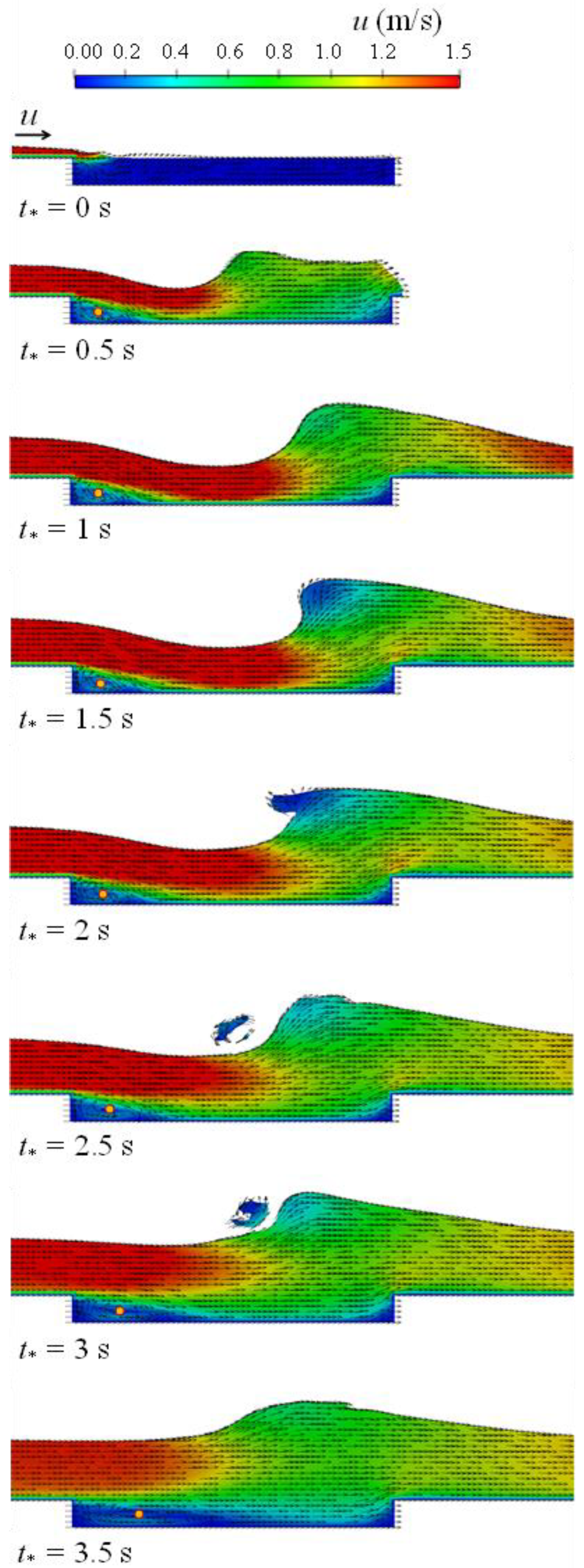
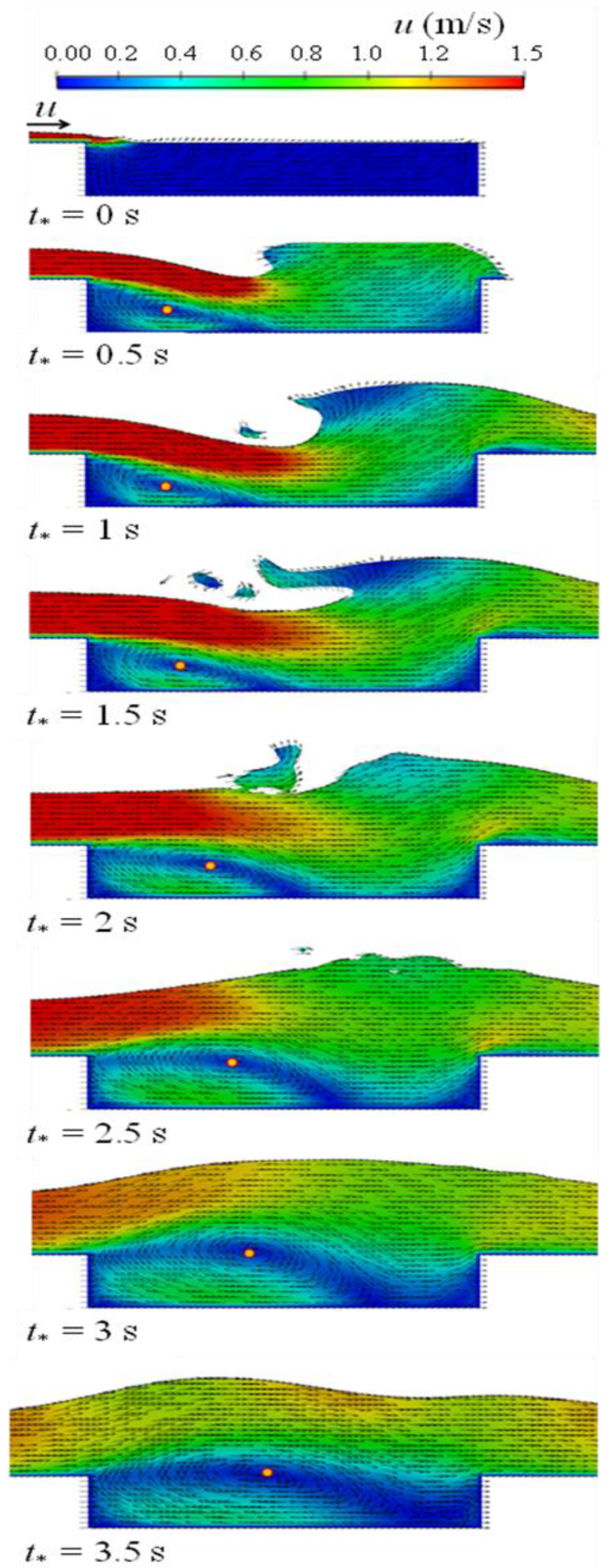
The time-history contour plots of the velocities of hydraulic bores passing over the mitigation canal were extracted from the validated numerical models in order to study the effect of canal depth on the hydrodynamics of a turbulent bore and its interaction with the canal. Figure 10 shows the time histories of the contour plots of the bore velocity and the velocity vector field of a turbulent bore, generated using an impoundment with a depth of do = 0.3 m, passing over a rectangular canal (w = 0.6 m, d = 0.05 m). It can be seen that the red area of the maximum bore velocity (i.e., u ≥ 1.5 m/s) decreases over time, indicating a significant momentum transfer due to the presence of the canal. The region of maximum bore velocity (i.e., u ≥ 1.5 m/s) did not reach the downstream end of the canal, indicating that the canal length is long enough to deflect the bore jet stream towards the bottom of the canal. At t⁎ = 0 s, the bore front reached the upstream of the canal, and the peak velocity jet stream reached the half-way point of the canal at t⁎ = 0.5 s. The maximum length of the jet stream occurred at a t⁎ between 1 s and 2.5 s. The eye of the vortex field formed in the vicinity of the upstream edge of the canal under the red area of the maximum bore velocity (i.e., u ≥ 1.5 m/s), as shown by the yellow spot in Figure 10. The vortex eye was formed 0.05 m from the upstream wall of the canal and moved slowly downstream as the bore passed over the canal. At t⁎ = 1.5 s, the maximum bore velocity reached the longest distance of 0.45 m from the upstream edge of the canal. Once the turbulent bore front passed the canal, the bore energy decreased, and the bore jet stream decayed. As a result, the peak velocity jet stream retreated back to the first half of the canal. The upward deflection of the peak velocity jet stream at t⁎ = 3.5 s increased the recirculation zone in the upstream edge of the canal and gradually moved the eye of the vortex upward, from 0.05 m to 0.12 m. Tidal currents usually generate river bores. Similar flows can be generated in controlled environments such as wave flumes. A number of experimental investigations have been conducted to determine some of the main features of hydraulic bores. The relatively slight discrepancy in the experiments could be partially attributed to the vorticity generated by the discharge method used to produce the undular bore. Vorticity, in particular, is a main factor which influenced the constant discharge bores. Some authors have suggested that bottom friction influences the emergence of an undular bore. If the conditions are suitable, a nearly constant profile of undulations can be observed in a river bore [52,53,54,55,56,57,58].
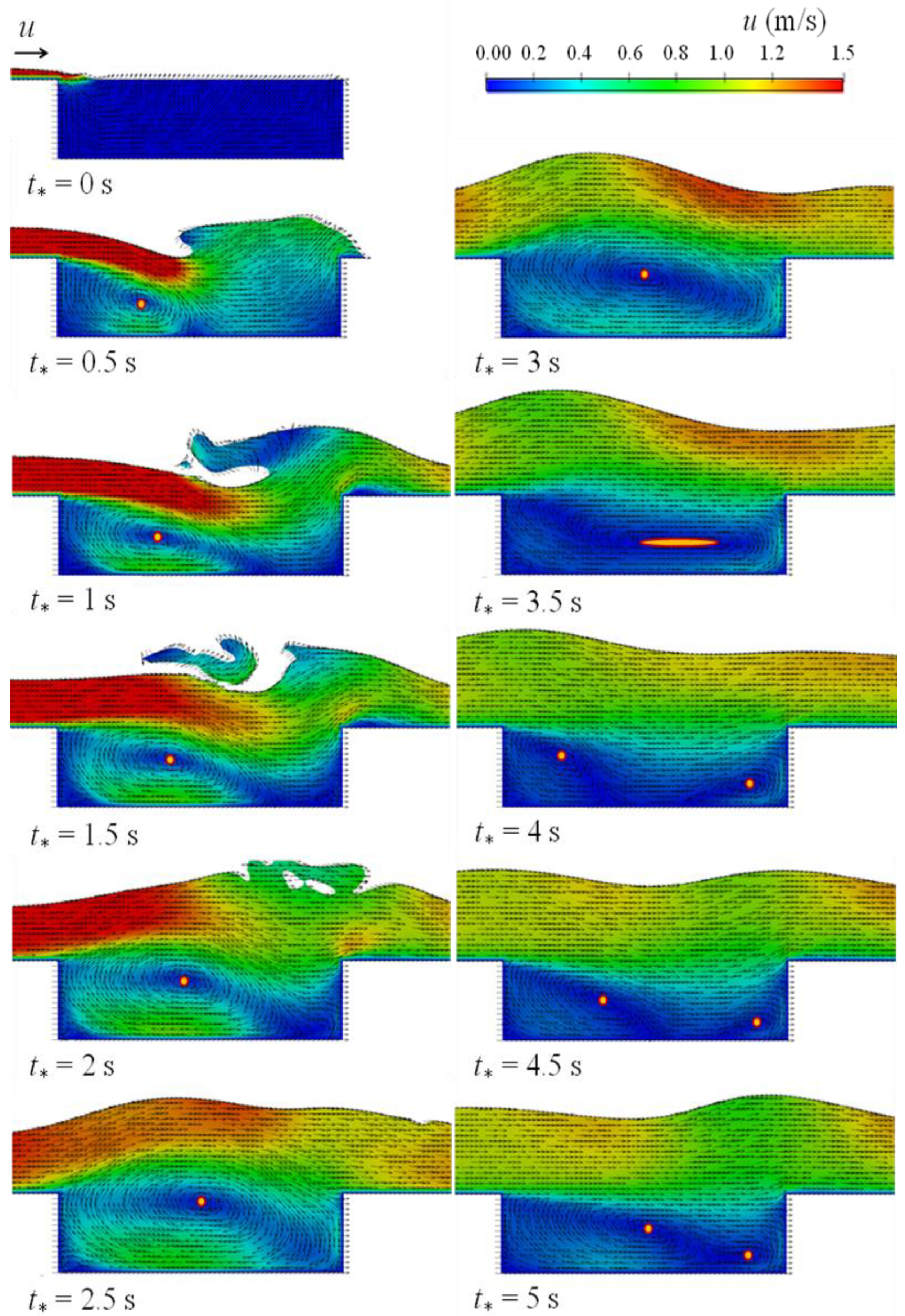
The contour plots of the bore velocities and velocity vector fields for turbulent bores with an impoundment depth of do = 0.3 m, passing over a medium-depth canal (d = 0.10 m) and a deep canal (d = 0.15 m), are shown in Figure 11 and Figure 12, respectively.
Similar to Figure 10, the maximum bore velocity was indexed at a velocity range of u ≥ 1.5 m/s. As can be seen, the jet stream of the peak velocity plunged downward into the canal and reached the half-way point of the canal at 0.5 s ≤ t⁎ ≤ 2.50 s. The penetration length of the jet stream with the maximum bore velocity decreased as the canal depth increased. In addition, the vortex eyes in the medium-depth (d = 0.10 m) and deep (d = 0.15 m) canals gradually moved downstream until they reached the longest distance from the upstream wall of the canals, i.e., 0.27 m at t⁎ = 3.5 s and 0.31 m at t⁎ = 3 s, respectively. The authors conclude that the location of the vortex eye as measured from the upstream wall of the canal increased with an increase in canal depth.
At t⁎ = 3.5 s, the vortex eye elongated as a result of water circulation through the entire width of the canal. At t⁎ ≥ 4.0 s, the vortex eye in the deep canal split into two vortices, and the velocity vectors show that the bore plunged downward into the middle of the canal. The new smaller vortices were generated in the vicinity of the upstream and downstream walls of the canal as the walls restricted the movement and propagation of the bore inside the canal. The vortex near the upstream wall started to move towards the downstream direction until it reached the middle of the canal at t⁎ = 5.0 s.
5. Discussion
The mitigation effects of a perpendicular canal on various dam-break waves were examined using laboratory experiments and numerical simulations. The effect of a mitigation canal on the wave hydrodynamics, namely the time histories of the water surface levels and velocities, was studied by employing a rectangular canal with a constant width of w = 0.6 m and three depths of d = 0.05 m, 0.10 m, and 0.15 m. The experimental results were also modelled with an OpenFoam multi-phase, three-dimensional numerical model. The differences between the maximum water depth predictions and measurements in the absence of a canal at WG (1.0 m upstream of the gate), US1 (0.20 m upstream of the canal), US2 (0.20 m downstream of the canal), and US3 (0.58 m downstream of the canal) were 4%, 10%, 6%, and 7%, respectively. Similarly, the performance of the validated numerical model in predicting the maximum water depth in the presence of a canal at WG, US1, US2, and US3 was 5%, 1%, 6%, and 9%, respectively. The performance of the validated numerical model in predicting the bore velocity at ADV1 (0.20 m upstream of the canal), ADV2 (0.20 m downstream of the canal), ADV3 (0.58 m downstream of the canal), and in the absence of a canal was 9.5%, 11%, and 11.5%, respectively. In the presence of a canal, the difference between the experimental and numerical results in velocity predictions at ADV1, ADV2, and ADV3 were 20%, 1%, and 17%, respectively.
The accuracy of the numerical models in predicting the time history of the bore water surface was found to be reasonable, within an error margin of approximately 5%. Three turbulence models were tested to predict the bore hydrodynamics when propagating over a canal. It was found that the classic k-ε turbulence model performed well, with an RMSE < 6.7% and a relative error of <8.4%. Both the numerical and experimental results showed that the depth of the canal plays a significant role in influencing bore wave hydrodynamics. As such, when considering the design of a mitigation canal, the interaction of the tsunami inundation bore with the canal depth must be taken into account. A suitable choice of canal geometry may considerably modify water levels and the associated turbulent bore velocity. A reduction of the bore velocity in particular leads to a reduction in the tsunami-induced momentum and the hydrodynamic loading of structures located near the canal.
The time history of the water surface showed that the quasi-steady state influence of a water surface profile, owing to the interaction of the passing bore with the canal, can reduce the bore momentum and energy and hence reduce the hydrodynamic loading on the other side of the canal. For the canal depth of d = 0.05 m, simulated streamlines near the canal bottom did not reach the level of the flume bed throughout the whole time history (t⁎ = 3.5 s), while for the canal depths of d = 0.10 m and d = 0.15 m, the simulated streamlines did reach the flume bed level. Streamline motion was also faster for the case of mitigation canals with greater depth.
The highest bore velocity decreased over time, suggesting a major reduction in momentum due to the presence of the canal. The penetration lengths of the jet stream with the highest bore velocity were reduced as the depth of the canal increased. The position of the eye of the vortex was located near the upstream wall of the canal; its size decreased as the canal depth decreased. It can therefore be concluded that as the canal depth increased, energy dissipation proportionally increased. This was inferred from the fact that the jet stream of the maximum bore velocity decreased as the canal depth increased due to the higher capacity of the deep canal to dissipate the energy generated by the bore–canal interaction. As the canal depth increased, the volume of water contributing to the eddy generation in the initial flow direction decreased; as a result, the distance of the vortex eye from the canal edge increased. In addition, two vortices formed at 4.0 s ≤ t⁎ ≤ 5.0 s for the deep (d = 0.15 m) canal after the original vortex eye stretched due to the circulation of the water in the canal. As a result, the original vortex separated into two smaller, separate vortices due to the bore plunging downward into the middle of the canal.
The bore front plunges into the canal, generates a high splash, interacts with the stagnant water in the canal, and then dissipates energy. Energy dissipation due to the turbulence generated by the interaction of the high-speed bore with the stagnant water is significant. In the presence of the canal, the bore’s impact on the canal results in the water propagating with a larger depth and a slower velocity as compared to the same conditions but in the absence of the canal. The time histories of the water surface level of the experimental and the numerical simulation results generally show good agreement as the developed numerical model simulates the turbulent kinetic energy dissipation occurring in the canal, which is triggered by the interaction between the bore and the stagnant water in the canal.
Finally, while the scope of this preliminary study has limitations, the authors conclude that mitigation canals have the potential to act as measures that reduce hydrodynamic loading on critical infrastructure located in nearshore areas.
6. Conclusions
- Three turbulence models were tested to predict the time history of the water level; they performed very well for the propagation of the bore over the flat flume bed and in the presence of the mitigation canal, with an RMSE < 6.7% and a Relative Error < 8.4%. The accuracy of numerical models in predicting the time history of the water surface profiles was found to be within an error of approximately 5%.
- The experimental and numerical results indicated that the maximum water levels increased and the maximum flow velocity decreased as the turbulent bore propagated over the canal in comparison to the case when the canal was not present. The tsunami bore front plunged into the canal, generating a high splash and interacting with the stagnant canal water. The energy of the tsunami bore front decreased significantly due to the turbulence generated by the dynamic impact of the bore.
- As the canal depth increased, its capability to suppress the momentum of the bore increased.
- The jet stream of the maximum bore velocity in shallow, medium-depth, and deep canals reached their longest distance from the upstream edge of the canal, with values of 0.45 m, 0.40 m, and 0.37 m, respectively. The energy dissipation of the bore plunging into the canal increased as the canal depth increased, and the jet stream of the maximum bore velocity decreased as the canal depth increased. Therefore, the maximum bore velocity jet stream for canals with depths of 0.05 m, 0.1 m, and 0.15 m extended to the furthest location downstream of the canal, with values of 0.45 m, 0.40 m, and 0.37 m, respectively.
- The location of the vortex eye for different canal depths gradually moved downstream until reaching distances of 0.12 m, 0.27 m, and 0.31 m from the upstream canal edge, for canal depths of 0.05 m, 0.1 m, and 0.15 m, respectively.
- The mitigation canals have the potential to act as measures that reduce hydrodynamic loading on critical infrastructure located in tsunami-prone areas. The incipient research proposed in study confirms some of the field observations during tsunami forensic engineering events [59].
Author Contributions
Conceptualization, I.N. and A.M.; data curation, N.E.; formal analysis, N.E.; funding acquisition, I.N. and A.M.; investigation, N.E. and A.H.A.; methodology, I.N. and A.M.; project administration, I.N. and A.M.; resources, N.E.; software, N.E., I.N. and A.M.; supervision, I.N. and A.M.; validation, N.E.; visualization, N.E.; writing—original draft preparation, N.E., A.H.A., I.N. and A.M.; writing—review and editing, I.N. and A.M. All authors have read and agreed to the published version of the manuscript.
Funding
This research was supported by funding provided by Discovery (NSERC) Grants to Prof. Ioan Nistor (210282) and Prof. Majid Mohammadian (210717).
Institutional Review Board Statement
Not applicable.
Informed Consent Statement
Not applicable.
Data Availability Statement
Part or all of the data is available from the corresponding author upon request.
Conflicts of Interest
The authors declare no conflict of interest.
Nomenclature
The following symbols are used in this paper:
| B | flume width (m) |
| d | canal depth (m) |
| do | equivalent impoundment depth (m) |
| g | gravitational acceleration (m/s2) |
| h | water surface elevation (m) |
| L | reservoir length (m) |
| P | fluid pressure (Pa) |
| t | time since gate opening (s) |
| to | gate-opening time (s) |
| t⁎ | time since the bore front plunges into the canal (s) |
| To | non-dimensional removal time for the gate (-) |
| u | turbulent bore velocity (m/s) |
| u, v, w | components of velocity in the x-, y- and z-directions, respectively (m/s) |
| u′, v′, w′ | turbulent fluctuation of velocity in the x-, y- and z-directions, respectively (m/s) |
| components of mean velocity in the x-, y-, and z-directions, respectively (m/s) | |
| U | flow velocity (m/s) |
| w | canal width (m) |
| RMSE | root mean square error (%) (-) |
| α | phase fraction (-) |
| ρ | density of air-water mixture (kg/m3) |
| ρa | density of the air (kg/m3) |
| ρw | density of the water (kg/m3) |
References
- FEMAP646. Guidelines for Design of Structure for Vertical Evacuation from Tsunamis, 2nd ed.; Federal Emergency Management Agency: Redwood, CA, USA, 2012.
- Nistor, I.; Saatcioglu, M.; Ghobarah, A. The 26 December 2004 earthquake and tsunami-hydrodynamic forces on physical infrastructure in Thailand and Indonesia. In Proceedings of the Canadian Coastal Engineering Conference, Halifax, NS, Canada, 6–9 November 2005. CD-ROM. [Google Scholar]
- Nistor, I.; Palermo, D. Post-Tsunami Engineering Forensics: Tsunami Impact on Infrastructure—Lessons from 2004 Indian Ocean, 2010 Chile, and 2011 Tohoku Japan Tsunami Field Surveys. In Handbook of Coastal Disaster Mitigation for Engineers and Planners; Butterworth-Heinemann: Waltham, MA, USA, 2015; pp. 417–435. [Google Scholar] [CrossRef]
- Ghobarah, A.; Saatcioglu, M.; Nistor, I. The Impact of the 26 December 2004 Earthquake and Tsunami on Structures and Infrastructure. Eng. Struct. 2006, 28, 312–326. [Google Scholar] [CrossRef]
- Rajaie, M.; Azimi, A.H.; Nistor, I.; Rennie, C.D. Experimental investigations on hydrodynamic characteristics of tsunami-like hydraulic bores impacting a square structure. J. Hydraul. Eng. 2022, 148, 04021061. [Google Scholar] [CrossRef]
- Douglas, S. Numerical Modeling of Extreme Hydrodynamic Loading and Pneumatic Long Wave Generation: Application of a Multiphase Fluid Model. Ph.D. Thesis, University of Ottawa, Ottawa, ON, Canada, 2016. [Google Scholar]
- Ghodoosipour, B.; Stolle, J.; Nistor, I.; Mohammadian, A.; Goseberg, N. Experimental study on extreme hydrodynamic loading on pipelines. Part 1: Flow hydrodynamics. J. Mar. Sci. Eng. 2019, 7, 251. [Google Scholar] [CrossRef] [Green Version]
- Ghodoosipour, B.; Stolle, J.; Nistor, I.; Mohammadian, A.; Goseberg, N. Experimental study on extreme hydrodynamic loading on pipelines. Part 2: Induced force analysis. J. Mar. Sci. Eng. 2019, 7, 262. [Google Scholar] [CrossRef] [Green Version]
- Chanson, H. Tsunami surges on dry coastal plains: Application of dam break wave equations. Coast. Eng. J. 2006, 48, 355–370. [Google Scholar] [CrossRef] [Green Version]
- Nistor, I.; Palermo, D.; Nouri, Y.; Murty, T.; Saatcioglu, M. Tsunami-induced forces on structures. In Handbook of Coastal and Ocean Engineering; World Scientific: Singapore, 2009; pp. 261–286. [Google Scholar] [CrossRef]
- Sarjamee, S.; Nistor, I.; Mohammadian, A. Numerical Investigation of the Influence of Extreme Hydrodynamic Forces on the Geometry of Structures Using OpenFOAM. Nat. Hazards 2017, 87, 213–235. [Google Scholar] [CrossRef]
- Wüthrich, D.; Pfister, M.; Nistor, I.; Schleiss, A.J. Experimental study of tsunami-like waves generated with a vertical release technique on dry and wet beds. J. Waterw. Port Coast. Ocean. Eng. 2018, 144, 04018006. [Google Scholar] [CrossRef]
- Wüthrich, D.; Pfister, M.; Nistor, I.; Schleiss, A.J. Experimental study on the hydrodynamic impact of tsunami-like waves against impervious free-standing buildings. Coast. Eng. J. 2018, 60, 180–199. [Google Scholar] [CrossRef]
- Wüthrich, D.; Pfister, M.; Nistor, I.; Schleiss, A.J. Experimental study on forces exerted on buildings with openings due to extreme hydrodynamic events. Coast. Eng. 2018, 140, 72–86. [Google Scholar] [CrossRef]
- Asadollahi, N.; Nistor, I.; Mohammadian, A. Numerical investigation of tsunami bore effects on structures. Part I: Drag coefficients. Nat. Hazards 2019, 96, 285–309. [Google Scholar] [CrossRef]
- Asadollahi, N.; Nistor, I.; Mohammadian, A. Numerical investigation of tsunami bore effects on structures. Part II: Effects of bed condition on loading onto circular structures. Nat. Hazards 2019, 96, 331–351. [Google Scholar] [CrossRef]
- Madsen, P.A.; Fuhrman, D.R.; Schäffer, H.A. On the solitary wave paradigm for tsunamis. J. Geophys. Res. Ocean. 2008, 113, C12012. [Google Scholar] [CrossRef]
- Leal, J.G.; Ferreira, R.M.; Cardoso, A.H. Maximum Level and Time to Peak of Dam-Break Waves on Mobile Horizontal Bed. J. Hydraul. Eng. 2009, 135, 995–999. [Google Scholar] [CrossRef] [Green Version]
- Khankandi, A.; Tahershamsi, A.; Soares-Frazão, S. Experimental investigation of reservoir geometry effect on dam-break flow. J. Hydraul. Res. 2012, 50, 376–387. [Google Scholar] [CrossRef]
- Shafiei, S.; Melville, B.W.; Shamseldin, A.Y. Experimental investigation of tsunami bore impact force and pressure on a square prism. Coast. Eng. 2016, 110, 1–16. [Google Scholar] [CrossRef]
- Shafiei, S.; Melville, B.W.; Shamseldin, A.Y.; Beskhyroun, S.; Adams, K.N. Measurements of tsunami-borne debris impact on structures using an embedded accelerometer. J. Hydraul. Res. 2016, 54, 435–449. [Google Scholar] [CrossRef]
- Liu, H.; Liu, H.; Guo, L.; Lu, S. Experimental Study on the Dam-Break Hydrographs at the Gate Location. J. Ocean. Univ. China 2017, 16, 697–702. [Google Scholar] [CrossRef]
- Al-Faesly, T.; Palermo, D.; Nistor, I.; Cornett, A. Experimental modeling of extreme hydrodynamic forces on structural models. Int. J. Prot. Struct. 2012, 3, 477–505. [Google Scholar] [CrossRef]
- Stolle, J.; Ghodoosipour, B.; Derschum, C.; Nistor, I.; Petriu, E.; Goseberg, N. Swing gate generated dam-break waves. J. Hydraul. Res. 2019, 57, 675–678. [Google Scholar] [CrossRef]
- Crespo, A.J.; Gómez-Gesteira, M.; Dalrymple, R.A. Modeling dam break behavior over a wet bed by a SPH technique. J. Waterw. Port Coast. Ocean. Eng. 2008, 134, 313–320. [Google Scholar] [CrossRef]
- Duarte, R.; Ribeiro, J.; Boillat, J.L.; Schleiss, A. Experimental study on dam-break waves for silted-up reservoirs. J. Hydraul. Eng. 2011, 137, 1385–1393. [Google Scholar] [CrossRef]
- Oertel, M.; Bung, D.B. Initial stage of two-dimensional dam-break waves: Laboratory versus VOF. J. Hydraul. Res. 2012, 50, 89–97. [Google Scholar] [CrossRef]
- Aureli, F.; Dazzi, S.; Maranzoni, A.; Mignosa, P.; Vacondio, R. Experimental and numerical evaluation of the force due to the impact of a dam-break wave on a structure. Adv. Water Resour. 2015, 76, 29–42. [Google Scholar] [CrossRef]
- Arnason, H.; Petroff, C.; Yeh, H. Tsunami bore impingement onto a vertical column. J. Disaster Res. 2009, 4, 391–403. [Google Scholar] [CrossRef]
- Baldock, T.E.; Peiris, D.; Hogg, A.J. Overtopping of solitary waves and solitary bores on a plane beach. Proc. R. Soc. A Math. Phys. Eng. Sci. 2012, 468, 3494–3516. [Google Scholar] [CrossRef] [Green Version]
- von Häfen, H.; Goseberg, N.; Stolle, J.; Nistor, I. Gate-Opening Criteria for Generating Dam-Break Waves. J. Hydraul. Eng. 2019, 145, 04019002. [Google Scholar] [CrossRef]
- Lauber, G.; Hager, W.H. Experiments to dambreak wave: Horizontal channel. J. Hydraul. Res. 1998, 36, 291–307. [Google Scholar] [CrossRef]
- Sarjamee, S.; Nistor, I.; Mohammadian, A. Large eddy simulation of extreme hydrodynamic forces on structures with mitigation walls using OpenFOAM. Nat. Hazards 2017, 85, 1689–1707. [Google Scholar] [CrossRef]
- Nouri, Y.; Nistor, I.; Palermo, D.; Cornett, A. Experimental investigation of tsunami impact on free standing structures. Coast. Eng. J. 2010, 52, 43–70. [Google Scholar] [CrossRef]
- Al-Faesly, T.Q. Extreme Hydrodynamic Loading on Near-Shore Structures. Ph.D. Thesis, University of Ottawa, Ottawa, ON, Canada, 2016; p. 356. [Google Scholar]
- Tanaka, N. Vegetation bioshields for tsunami mitigation: Review of effectiveness, limitations, construction, and sustainable management. Landsc. Ecol. Eng. 2009, 5, 71–79. [Google Scholar] [CrossRef] [Green Version]
- Fadly, U.; Murakami, K. Study on reducing tsunami inundation energy by the modification of topography based on local wisdom. J. Jpn. Soc. Civ. Eng. Ser. B3 (Ocean. Eng.) 2012, 68, 66–71. [Google Scholar] [CrossRef] [Green Version]
- Dao, N.X.; Adityawan, M.B.; Tanaka, H. Sensitivity analysis of shore-parallel canal for tsunami wave energy reduction. J. Jpn. Soc. Civ. Eng. Ser. B3 (Ocean. Eng.) 2013, 69, 401–406. [Google Scholar] [CrossRef] [Green Version]
- Elsheikh, N.; Azimi, A.H.; Nistor, I.; Mohammadian, A. Experimental Investigations of Hydraulic Surges Passing Over a Rectangular Canal. J. Earthq. Tsunami 2020, 14, 2040004. [Google Scholar] [CrossRef]
- St-Germain, P.; Nistor, I.; Townsend, R.; Shibayama, T. Smoothed-particle hydrodynamics numerical modeling of structures impacted by tsunami bores. J. Waterw. Port Coast. Ocean. Eng. 2014, 140, 66–81. [Google Scholar] [CrossRef]
- Watanabe, S.A.; Mikami, T.; Shibayama, T. Laboratory Study on Tsunami Reduction Effect of Teizan Canal. In Proceedings of the 6th International Conference on the Application of Physical Modelling in Coastal and Port Engineering and Science (Coastlab16), Ottawa, ON, Canada, 10–13 May 2016; pp. 1–6. [Google Scholar]
- Rahman, M.M.; Schaab, C.; Nakaza, E. Experimental and numerical modeling of tsunami mitigation by canals. J. Waterw. Port Coast. Ocean. Eng. 2017, 143, 04016012. [Google Scholar] [CrossRef]
- St-Germain, P.; Nistor, I.; Townsend, R. Numerical modeling of the impact with structures of tsunami bores propagating on dry and wet beds using the SPH method. Int. J. Prot. Struct. 2012, 3, 221–255. [Google Scholar] [CrossRef]
- Douglas, S.; Nistor, I. On the effect of bed condition on the development of tsunami-induced loading on structures using OpenFOAM. Nat. Hazards 2015, 76, 1335–1356. [Google Scholar] [CrossRef]
- OpenFOAM. OpenFOAM: The Open Source CFD Toolbox. Available online: http://foam.sourceforge.net/docs/Guides-a4/UserGuide.pdf (accessed on 14 July 2021).
- Sarjamee, S. Numerical Modelling of Extreme Hydrodynamic Loading on Coastal Structures. Master’s Thesis, University of Ottawa, Ottawa, ON, Canada, 2016. [Google Scholar]
- Versteeg, H.K.; Malalasekera, W. An Introduction to Computational Fluid Dynamics: The Finite Volume Method, 2nd ed.; Pearson Education Ltd.: Harlow, UK; New York, NY, USA, 2007. [Google Scholar]
- Heyns, J.A.; Malan, A.G.; Harms, T.M.; Oxtoby, O.F. Development of a compressive surface capturing formulation for modelling free-surface flow by using the volume-of-fluid approach. Int. J. Numer. Methods Fluids 2013, 71, 788–804. [Google Scholar] [CrossRef]
- Ferziger, J.H.; Perić, M. Computational Methods for Fluid Dynamics; Springer: Berlin/Heidelberg, Germany, 2002. [Google Scholar]
- Azimi, A.H.; Zhu, D.Z.; Rajaratnam, N. Effect of particle size on the characteristics of sand jet in water. J. Eng. Mech. 2011, 137, 822–834. [Google Scholar] [CrossRef]
- Azimi, A.; Zhu, D.Z.; Rajaratnam, N. Computational Investigation on Vertical Slurry Jets. Int. J. Multiph. Flow 2012, 47, 94–114. [Google Scholar] [CrossRef]
- Shugan, I.V.; Chen, Y.-Y.; Hsu, C.-J. Experimental and Theoretical Study on Flood Bore Propagation and Forerunner Generation in Dam-Break Flow. Phys. Wave Phenom. 2020, 28, 274–284. [Google Scholar] [CrossRef]
- Vargas-Magaña, R.M.; Marchant, T.R.; Smyth, N.F. Numerical and analytical study of undular bores governed by the full water wave equations and bidirectional Whitham–Boussinesq equations. Phys. Fluids 2021, 33, 067105. [Google Scholar] [CrossRef]
- El, G.A.; Grimshaw, R.H.J.; Kamchatnov, A.M. Analytic model for a weakly dissipative shallow-water undular bore. Chaos Interdiscip. J. Nonlinear Sci. 2005, 15, 037102. [Google Scholar] [CrossRef] [Green Version]
- Amaechi, C.V.; Wang, F.; Ye, J. Mathematical Modelling of Bonded Marine Hoses for Single Point Mooring (SPM) Systems, with Catenary Anchor Leg Mooring (CALM) Buoy Application—A Review. J. Mar. Sci. Eng. 2021, 9, 1179. [Google Scholar] [CrossRef]
- Hatland, S.D.; Kalisch, H. Wave breaking in undular bores generated by a moving weir. Phys. Fluids 2019, 31, 033601. [Google Scholar] [CrossRef] [Green Version]
- El, G.A.; Grimshaw, R.H.J.; Kamchatnov, A.M. Wave Breaking and the Generation of Undular Bores in an Integrable Shallow Water System. Stud. Appl. Math. 2005, 114, 395–411. [Google Scholar] [CrossRef]
- El, G.A.; Khodorovskii, V.V.; Tyurina, A.V. Undular bore transition in bi-directional conservative wave dynamics. Phys. D Nonlinear Phenom. 2005, 206, 232–251. [Google Scholar] [CrossRef]
- Chock, G.; Roberson, I.; Kriebel, D.; Francis, M.; Nistor, I. Tohoku Japan Tsunami of March 11, 2011—Performance of Structures under Tsunami Loads; ASCE/SEI Report; ASCE: Reston, VA, USA, 2013; p. 359. [Google Scholar]
Figure 1.
Image of tsunami propagating over a canal during the 2011 Japan Tsunami event Reprinted with permission from [5] (2022, ASCE).
Figure 1.
Image of tsunami propagating over a canal during the 2011 Japan Tsunami event Reprinted with permission from [5] (2022, ASCE).

Figure 2.
Schematic of experimental setup and coordinate system: (a) side view; (b) top view (not at scale).
Figure 2.
Schematic of experimental setup and coordinate system: (a) side view; (b) top view (not at scale).

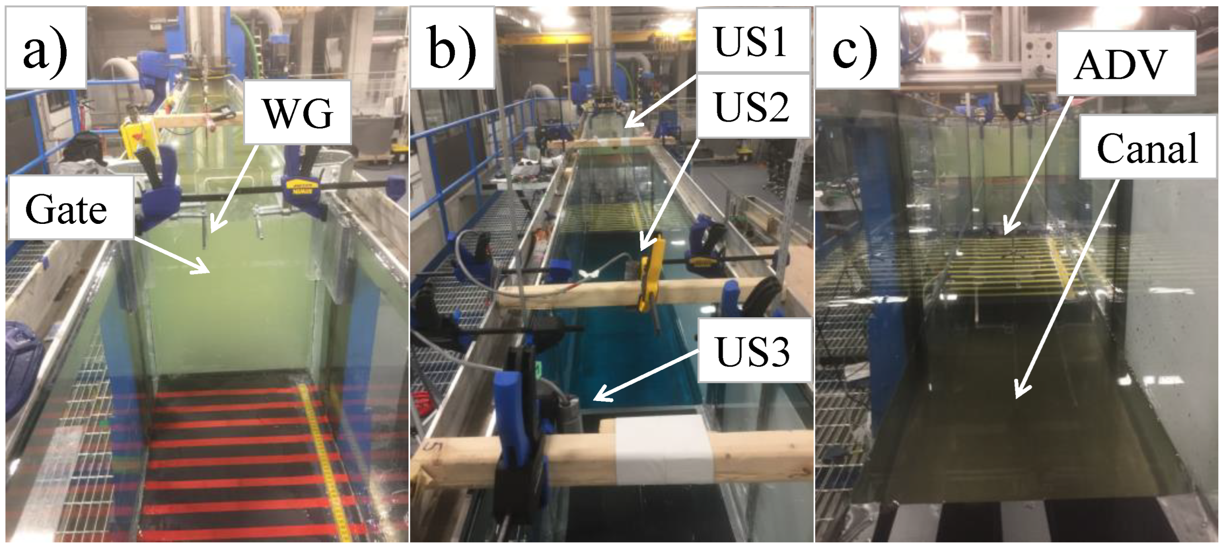
Figure 3.
Laboratory experimental setup: (a) upstream view of the flume and the vertical gate; (b) positions of the ultrasonic depth sensors (US) in the flume; (c) upstream view of the canal and the ADV probe.
Figure 3.
Laboratory experimental setup: (a) upstream view of the flume and the vertical gate; (b) positions of the ultrasonic depth sensors (US) in the flume; (c) upstream view of the canal and the ADV probe.

Figure 4.
Computational domain and three-dimensional water surface profile: (a) computational domain of the full channel; (b) mesh resolution of the reservoir in the initial condition; (c) mesh resolution in the canal; (d) three-dimensional water surface profile at t⁎ = 0.25 s; (e) three-dimensional water surface profile at t⁎ = 0.5 s. t⁎ is the time when the bore front reaches the canal.

Figure 5.
Effect of different turbulence models on the prediction of the time history of the water surface profiles, and comparisons of numerical results with laboratory measurements for do = 0.4 m. Left column shows the time history of the water surface profiles over the horizontal bed section, while the right column shows the time history of the water surface profiles over a rectangular canal (w = 0.6 m, d = 0.15 m): (a) WG; (b) US1; (c) US2; (d) US3.

Figure 6.
Effect of different turbulence models on the prediction of bore velocity profiles, and comparisons of the numerical results with laboratory measurements for do = 0.4 m. Left column shows the bore velocity profiles over a horizontal surface, and right column shows the bore velocity profiles over a rectangular canal (w = 0.6 m, d = 0.15 m): (a) ADV1; (b) ADV2; (c) ADV3.

Figure 7.
Time history of water surface profiles of a bore from an impoundment with a depth of do = 0.3 m, passing over a canal with a width of w = 0.6 m and a depth of d = 0.05 m: (a) side-view images; (b) simulated water surface profile and streamlines.
Figure 7.
Time history of water surface profiles of a bore from an impoundment with a depth of do = 0.3 m, passing over a canal with a width of w = 0.6 m and a depth of d = 0.05 m: (a) side-view images; (b) simulated water surface profile and streamlines.

Figure 8.
Time history of water surface profiles of a bore from an impoundment with a depth of do = 0.3 m, passing over a canal with a width of w = 0.6 m and a depth of d = 0.10 m: (a) side-view images; (b) simulated water surface profile and streamlines.
Figure 8.
Time history of water surface profiles of a bore from an impoundment with a depth of do = 0.3 m, passing over a canal with a width of w = 0.6 m and a depth of d = 0.10 m: (a) side-view images; (b) simulated water surface profile and streamlines.

Figure 9.
Time history of water surface profiles of a bore from an impoundment with a depth of do = 0.3 m, passing over a canal with a width of w = 0.6 m and a depth of d = 0.15 m: (a) side-view images; (b) simulated water surface profile and streamlines.
Figure 9.
Time history of water surface profiles of a bore from an impoundment with a depth of do = 0.3 m, passing over a canal with a width of w = 0.6 m and a depth of d = 0.15 m: (a) side-view images; (b) simulated water surface profile and streamlines.

Figure 10.
Variations of the contour plots of velocity and velocity vector fields with time, for a bore from an impoundment with a depth of do = 0.3 m, passing over a canal with a width of w = 0.6 m and a depth of d = 0.05 m. The dots in the contour plots show the eye of the vortex.
Figure 10.
Variations of the contour plots of velocity and velocity vector fields with time, for a bore from an impoundment with a depth of do = 0.3 m, passing over a canal with a width of w = 0.6 m and a depth of d = 0.05 m. The dots in the contour plots show the eye of the vortex.

Figure 11.
Variations of the contour plots of velocity and velocity vector fields with time, for a bore from an impoundment with a depth of do = 0.3 m, passing over a canal with a width of w = 0.6 m and a depth of d = 0.10 m. The dots in the contour plots show the eye of the vortex.
Figure 11.
Variations of the contour plots of velocity and velocity vector fields with time, for a bore from an impoundment with a depth of do = 0.3 m, passing over a canal with a width of w = 0.6 m and a depth of d = 0.10 m. The dots in the contour plots show the eye of the vortex.

Figure 12.
Variations of the contour plots of velocity and velocity vector fields with time, for a bore from an impoundment with a depth of do = 0.3 m, passing over a canal with a width of w = 0.6 m and a depth of d = 0.15 m. The dots in the contour plots show the eyes of the vortices.
Figure 12.
Variations of the contour plots of velocity and velocity vector fields with time, for a bore from an impoundment with a depth of do = 0.3 m, passing over a canal with a width of w = 0.6 m and a depth of d = 0.15 m. The dots in the contour plots show the eyes of the vortices.


Table 1.
Parameters of the performed tests.
| Test No. | Test Name | do (m) | w (m) | d (m) | w/d |
|---|---|---|---|---|---|
| 1 | F-0.3 | 0.30 | 0 | 0 | 0 |
| 2 | F-0.4 | 0.40 | 0 | 0 | 0 |
| 3 | C-0.3–4 | 0.30 | 0.60 | 0.15 | 4 |
| 4 | C-0.3–6 | 0.30 | 0.60 | 0.10 | 6 |
| 5 | C-0.3–12 | 0.30 | 0.60 | 0.05 | 12 |
| 6 | C-0.4–4 | 0.40 | 0.60 | 0.15 | 4 |
Table 2.
Percentage error values of the compared numerical results versus laboratory measurements of the maximum water surface levels and velocities.
Table 2.
Percentage error values of the compared numerical results versus laboratory measurements of the maximum water surface levels and velocities.
| Parameter | Location | In the Absence of the Canal (%) | In the Presence of the Canal (%) |
|---|---|---|---|
| WSL | WG | 4 | 5 |
| US1 | 10 | 1 | |
| US2 | 6 | 6 | |
| US3 | 7 | 9 | |
| Velocity | ADV1 | 9.5 | 20 |
| ADV2 | 11 | 1 | |
| ADV3 | 11.5 | 17 |
Publisher’s Note: MDPI stays neutral with regard to jurisdictional claims in published maps and institutional affiliations. |
© 2022 by the authors. Licensee MDPI, Basel, Switzerland. This article is an open access article distributed under the terms and conditions of the Creative Commons Attribution (CC BY) license (https://creativecommons.org/licenses/by/4.0/).
Share and Cite
MDPI and ACS Style
Elsheikh, N.; Nistor, I.; Azimi, A.H.; Mohammadian, A. Tsunami-Induced Bore Propagating over a Canal—Part 1: Laboratory Experiments and Numerical Validation. Fluids 2022, 7, 213. https://0-doi-org.brum.beds.ac.uk/10.3390/fluids7070213
AMA Style
Elsheikh N, Nistor I, Azimi AH, Mohammadian A. Tsunami-Induced Bore Propagating over a Canal—Part 1: Laboratory Experiments and Numerical Validation. Fluids. 2022; 7(7):213. https://0-doi-org.brum.beds.ac.uk/10.3390/fluids7070213
Chicago/Turabian StyleElsheikh, Nuri, Ioan Nistor, Amir H. Azimi, and Abdolmajid Mohammadian. 2022. "Tsunami-Induced Bore Propagating over a Canal—Part 1: Laboratory Experiments and Numerical Validation" Fluids 7, no. 7: 213. https://0-doi-org.brum.beds.ac.uk/10.3390/fluids7070213