

Efficient Scale-Resolving Simulations of Open Cavity Flows for Straight and Sideslip Conditions

Institute for Applied Mathematics and Scientific Computing, Department of Aerospace Engineering, University of the Bundeswehr Munich, 85577 Neubiberg, Germany
*
Author to whom correspondence should be addressed.
Fluids 2023, 8(8), 227; https://0-doi-org.brum.beds.ac.uk/10.3390/fluids8080227
Submission received: 8 July 2023
/
Revised: 29 July 2023
/
Accepted: 3 August 2023
/
Published: 8 August 2023
(This article belongs to the Special Issue Recent Advances in Aerodynamics and Aeroacoustics: Towards Greener Aviation)
Abstract
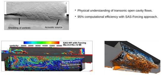
:This study aims to facilitate a physical understanding of resonating cavity flows with efficient numerical treatments of turbulence. It reinforces the efficiency and affordability of scale-adaptive numerical techniques for simulating open cavity flows with a separated shear layer consisting of a wide range of flow scales. Visualization of the resonant modes occurring due to the acoustic feedback loop aids in a better understanding of large-scale flow oscillations. Under this scope, scale-adaptive simulation (SAS) based on the k- SST RANS model with different turbulence treatments has been studied for an open cavity configuration with a length-to-depth ratio of featuring Mach number () and Reynolds number () . It is shown that the essential cavity flow physics has been captured using the SAS approach with more than improved computational efficiency compared to commonly used hybrid RANS-LES approaches. In addition, wall-modeled SAS when supplemented with an artificial forcing concept to trigger the model provides very good spectral estimates comparable with hybrid RANS-LES results. Following the validation of numerical approaches, the directional dependence of the cavity resonance is investigated under asymmetric flow conditions, and spanwise interference of waves due to the lateral walls of the cavity has been observed.
1. Introduction
Separated flow from the front edge of an open cavity configuration impinges on the rear wall. The impingement location on the rear wall acts as an acoustic source to initiate sustained flow oscillations inside the cavity [1]. Free-stream flow over the cavity, a shear layer and turbulent fluctuations contribute to a typical acoustic spectrum consisting of broadband noise and narrow-band tones. The high-amplitude narrow-band tones are attributed to Rossiter modes. Rossiter described the mechanism of distinct modes appearing in the open cavity and postulated a semi-empirical model to estimate the frequencies at which the modes occur [2]. He devised the oscillation model (Equation (1)) based on the observation that the downstream convection of vortices from the shear layer leads to the impingement of vortices at the downstream edge, generating acoustic waves. The generated acoustic waves travel upstream exciting further disturbances in the shear layer, leading to a self-sustained oscillation process.
where f is the frequency, is the free-stream velocity, L is the length of the cavity, m is the Rossiter mode number, is the phase delay constant with the value of [3], D is the depth of the cavity, is the Mach number and is the ratio of the convection velocity of the vortical structures to the free-stream velocity [2].
In the literature, there exists an ample number of cavity studies, discussing the effect of different parameters on the acoustic spectrum, namely the length-to-depth ratio, Reynolds number and presence of stores from subsonic to supersonic flow conditions [4,5,6]. Furthermore, some studies have reported on the understanding of the resonance process, which has been observed to be predominantly 2D in nature [7]. Gloerfelt et al. [8] observed the mechanism responsible for the lower frequency range, suggesting evidence of the possibility of mode-switching and strong coupling between the shear layer from the front edge and the recirculation region developed in the cavity. Wagner et al. [9] showed the correlation of large-scale flow oscillations to the first Rossiter mode, while higher-order modes were correlated to the coherent structures generated in the shear layer. Rowley et al. [10] conducted analyses that reveal a transition in the behavior of supersonic cavity flows. For shorter cavities and lower Mach numbers, a shear-layer mode dominates, while for longer cavities and higher Mach numbers, a wake mode becomes prevalent. The shear-layer mode is notably distinguished by the acoustic feedback process, as described by Rossiter. Disturbances in the shear layer align closely with predictions based on a linear stability analysis of the Kelvin–Helmholtz mode. On the other hand, the wake mode is characterized by the presence of large-scale vortex shedding, with the Strouhal number remaining independent of the Mach number.
Although many studies have been published on open cavity flows, there have been hardly any studies discussing the 3D effect from the lateral walls. Most of the studies cover symmetric flow conditions, whereas less attention to the modulation of resonant modes due to lateral walls is given. The aim of the current study is twofold. One is investigating the effect of asymmetric flow conditions on the cavity flow features, such as the resonant modes. The second is addressing the efficiency of treating turbulence so the computing effort can be reduced for industrial use. Highly resolving turbulence approaches, such as direct numerical simulation (DNS) and large eddy simulation (LES), are improbable to be used in industrial applications for high Reynolds number flows. Therefore, many of the cavity studies are focused on different ways of treating the turbulence. Chang et al. [11] studied 3D incompressible flow past an open cavity by modeling the entire range of the turbulent spectrum using the Spalart–Allmaras (SA) model. They showed good predictions of the mean velocity field by URANS and a scale-resolving simulation, whereas the turbulent quantities of URANS were shown to deviate from LES and the experimental results. Due to the nature of the URANS formulation, the method has an inherent inability to detect modes accurately. Therefore, a number of studies have been dedicated to scale-resolving turbulence models.
Nayyar et al. [12] showed the superior performance of the LES and detached eddy simulation (DES) models in predicting the noise level, frequency content and velocity profiles inside the cavity with and in comparison to the URANS approach. They showed that over-predicted spectral values are a common occurrence for most URANS computations. To achieve a reasonable behavior with URANS, some studies, such as Stanek et al. [13], have tried to limit the production of eddy viscosity based on the values produced along the boundary layer, without which hardly any oscillatory behavior was seen.
Wang et al. [14] performed numerical investigations to analyze oscillations in supersonic open cavity flows using a hybrid RANS-LES approach. Subsequently, simulations are carried out to identify and analyze the different oscillation regimes and feedback mechanisms present in the supersonic cavity flows. The characteristics of the oscillations in the flow of are captured in the calculation, wherein a mixed shear-layer/wake oscillation mode is observed to occur alternately.
Considering the expensive nature of the LES and DES models for 3D industrial computations, the focus now has been set on efficiently capturing the resonant modes. Girimaji et al. [15] evaluated the scale-adaptive simulation (SAS) of M219 cavity flows for transonic flow conditions and achieved computational efficiency relative to DES simulations. As the SAS model depends on inherent flow fluctuations to resolve the turbulence, the model might not resolve turbulence in quasi-steady conditions. Therefore, an improved version of the SAS model with artificial forcing (SAS-F) has been proposed by Menter et al. [16], where flow fluctuations are introduced based on the modeled turbulent length and time scales, which leads to the resolution of the turbulence field. This study applies the SAS-F model to fundamental planar flow applications, such as channel and backward-facing step configurations.
In the author’s previous study [17], the open cavity configuration presented in the work by Mayer et al. [18] has been studied numerically using the DLR-TAU code [19] for transonic flow conditions and supersonic conditions using a hybrid RANS-LES approach based on Spalart–Allmaras based on the improved delayed DES (SA-IDDES) model. Further studies [20,21] featured preliminary works on the different wall treatments in the framework of scale-adaptive simulation (SAS) towards reducing the computational cost of simulating cavity flows maintaining good accuracy relative to the hybrid RANS-LES results and experimental data. The current work focuses on the detailed investigations of the SAS approach, including the synthetic forcing technique for predicting spectra for straight flow conditions [22]. The configuration is then further studied under sideslip flow conditions to understand the directional impact of flow processes on the resonant modes and their modulations. Investigations into the 3D visualization of the resonant modes and performance of the SAS approaches with different numerical treatments are featured in this article. To realize the goals of this study, the open cavity configuration with opened doors at the sides [18] has been investigated numerically at transonic flow conditions of and using scale-resolving turbulence models such as SA-IDDES and SAS. The results of the SA-IDDES model supplemented with a wall function approach (DES-WF) have been used as a reference for the different SAS investigations, which include the wall-resolved (SAS-WR), the wall-modeled (SAS-WF) and the artificially-forced and wall-modeled SAS (SAS-F) variants. In addition to validating the different SAS variants for the symmetric flow case, the cavity has been studied further under the sideslip condition, with an angle of sideslip () with the SAS-WR approach to investigate the directional effects on the cavity flow features.
2. Cavity Model and Mesh
2.1. Description of the Cavity
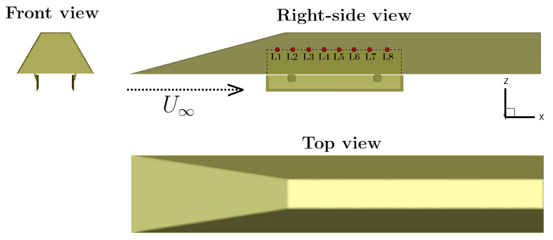
A cuboid cavity with a length-to-depth ratio of and length-to-width ratio of is cut into a flat side of a test rig at a certain distance from its sharp leading edge and on the center line (see Figure 1). The doors, which are connected to the rig plate, are placed on either side of the cavity with a positive Z pointing into the cavity. The experimental survey conducted by Mayer et al. [18] had probes placed at equidistant locations along the cavity ceiling, named L1 to L8, with the flow direction from the sharp leading edge of the rig towards the cavity. The flat plate upstream of the cavity is long enough to obtain a fully developed turbulent boundary layer before reaching the cavity.
2.2. Mesh
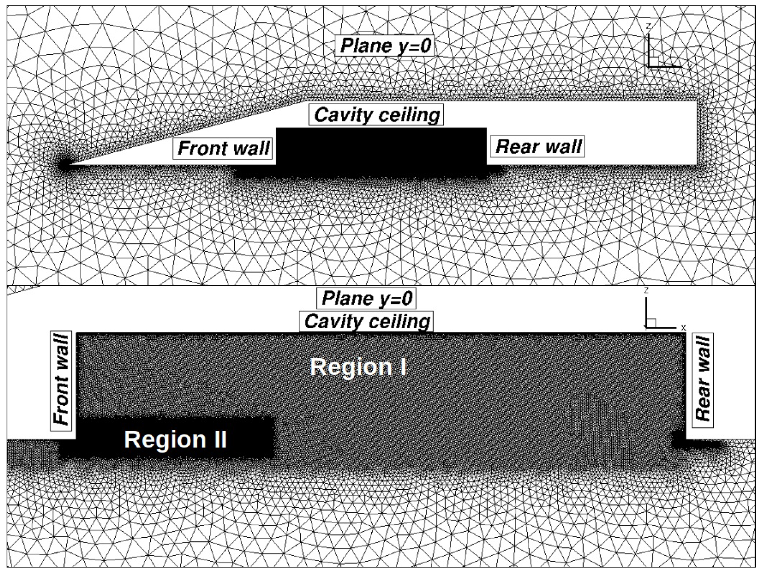
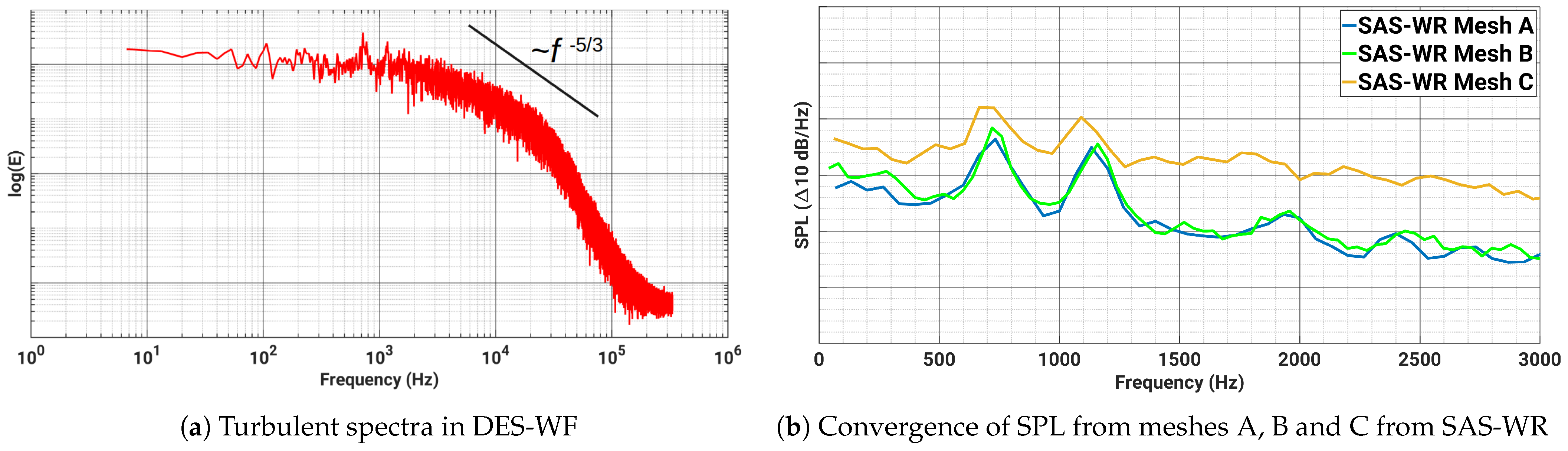
The numerical mesh used for all the turbulence models is of an unstructured type. The surface of the cavity walls, doors and the plate of the rig where the cavity is cut is composed of triangles and quadrilaterals. To cover the boundary layer over the flat plate leading to the cavity, the surface elements follow up to 35 layers of prism and hexahedral elements in the case of wall-resolved simulation and up to 10 layers in the case of wall-modeled simulation with as the total thickness of the layers for the considered flow conditions. The sharp leading edge of the rig has been refined to avoid the introduction of mesh-dependent errors that could be convected and affect the flow over the cavity. The other regions of the sphere-shaped computational domain with a diameter as high as are composed of unstructured elements with tetrahedral and pyramidal cells. The cavity ceiling near the front wall has lower values of compared to the aft part of the cavity, yet the number of prism layers has been kept the same. The model has been meshed in half and mirrored about the symmetry axis so that asymmetric grid effects are effectively avoided. The local regions in and around the cavity have been meshed based on the integral scale estimates obtained from the k- SST model. A total of 2–3 cells per integral length scale have been used to resolve the shear layer, and the resulting local mesh distribution is shown in Figure 2, where region I has cells with dimensions in the range of , whereas the cells in region II are half as big. For DES-WF the mesh resolution has been chosen by demonstrating the existence of a Kolmogorov inertial range [23], which extends roughly over one order of magnitude based on the turbulence in the shear layer. This condition has been verified in the shear layer, which can be seen in Figure 3a. The DES-WF mesh is composed of grid nodes and surface elements. Moreover, it has been observed that refining the entire shear layer does not provide further benefits for the prediction of resonance spectra.
Unlike DES-WF, regions I and II have the same mesh resolution, and the scale-resolving capability of SAS does not explicitly depend on the cell resolution, but on the scale (see Section 3.2). To achieve sufficiently resolved turbulence in the cavity, the cell size has been chosen based on a mesh convergence study. Three meshes, A, B and C, of increasing cell sizes by a factor of in each direction within the cavity have been chosen, which consist of , and million nodes, respectively (see Table 1). The wall-normal resolution has been the same for all of the meshes with of the first cell less than . The SPL spectra are very sensitive to the global mesh characteristics and resolution of the shear layer near the front edge and, therefore, are chosen for illustrating mesh convergence. The resulting spectra from SAS-WR on the three meshes are shown in Figure 3b. According to the results, mesh B has been chosen to perform the SAS-WR simulation. Overall, the SAS-WR mesh with prism cells contains around grid nodes. In SAS-WF and SAS-F, the resolution in the cavity is the same as in SAS-WR with of the first element greater than 100, whereby the resulting mesh has the advantage of using only 50% of the prism cells compared to the SAS-WR mesh with grid nodes. Table 2 summarizes the mesh parameters used for all of the simulation method variants in this study.
3. Simulation Methodologies
In this study, a three-dimensional, parallel, hybrid, finite volume code developed by the German Aerospace Center, DLR-TAU ([19]), has been used to carry out the numerical simulations for solving the compressible Navier-Stokes formulation, which has been written in a conservative form as follows.
where
The flux density tensor is composed of the flux vectors in the three coordinate directions:
The viscous and the inviscid fluxes in the x-direction:
The pressure field p is computed from the equation of state for a perfect gas (7)
In Equations (2)–(7), is density, T is temperature, H is enthalpy, V is an arbitrary control volume, t is time, is the ratio of specific heats, is an outer normal vector, is shear stress tensor, E is the total energy per unit mass and are instantaneous velocity components in directions with unit vectors , respectively.
Since an open cavity configuration features a complex flow pattern with a range of turbulent and acoustic scales, a high degree of turbulence resolution is preferred in the numerical simulations, and, therefore, different numerical treatments of turbulence have been applied in this study, which will be introduced briefly in this section.
3.1. Hybrid RANS-LES Approach
After the first promising results of this cavity configuration were published in a previous study [17], some of the numerical settings used have been optimized in the present work. By applying matrix dissipation [24] in this study, the artificial dissipation is reduced in order to prevent excessive damping of the resolved turbulent structures.
The DES-WF method is based on the SAneg model [25], which models the transport equation for the eddy viscosity and is written as follows [26].
The turbulent eddy viscosity is computed from:
where
The production term and the destruction term are:
Additional definitions are given by the following equations:
where and are model constants, , d is the distance to the nearest wall and is the shielding function designed to be unity in the LES region and zero elsewhere.
3.2. Scale-Adaptive Approach
Although all RANS models have the potential to be solved in an unsteady manner (URANS), conventional URANS models are known to lack spectral content, even when the grid and time step resolutions are adequate. This limitation has been attributed to high turbulent viscocities that reflect the averaging in the theoretical derivation of the RANS equations, which effectively removes all turbulence information from the velocity field. The SAS model can be considered as a URANS model with a scale-resolving capability, which can show LES-like behavior. Unlike LES, it also remains well-defined if the mesh cells become coarser. This makes it attractive in the present application, where the aero-acoustic effects are mostly affected by larger turbulent scales, which, in turn, need to be predicted accurately.
The work by Menter et al. [16] suggests a modified turbulence model that adds a source term based on the local von Karman length scale into the dissipation rate transport equation to only resolve turbulence where significant fluctuations exist and can be resolved by the mesh. This scale-resolving technique with the standard k- SST model [27] as the base model has been used in the present study. The source term is added in the transport equation for the turbulence eddy frequency which is defined in Einstein’s notations, as shown in Equation (14).
with , and and:
with and .
3.3. Wall Treatment
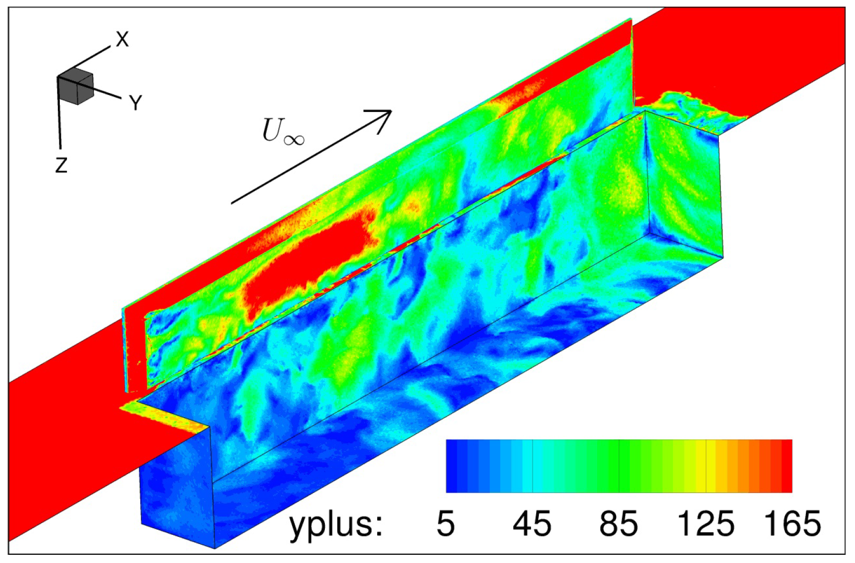
In this study, wall functions based on the universal law of the wall are employed for the DES-WF, SAS-WF and SAS-F simulations, whereas the low-Re boundary condition is used for the SAS-WR simulation. The aim of grid-independent wall functions is to provide a boundary condition at solid walls that enables flow solutions independently of the location of the first grid node above the wall. The RANS equations are solved only down to the first grid node above the wall and are matched there with an adaptive wall function solution. The matching condition (Equation (15)) makes sure that the wall-parallel components of the RANS solution and the wall function are equal at the wall distance , which is then solved for the friction velocity using Newton’s method. The shear stress is then prescribed at the wall node. Figure 4 shows the instantaneous non-dimensional wall distance distribution in the case of the DES-WF simulation.
3.4. Artificial Forcing
In principle, the SAS approach thrives under the presence of significant flow fluctuations. As will be shown in Section 4, wall functions tend to damp the fluctuations close to the wall, and this results in the inability of the model to produce enough fluctuations; eventually, the SAS model becomes dormant when wall functions are used, resulting in a URANS solution with fully modeled turbulence. Therefore, to increase the resolution capability of the SAS model in the shear layer, an investigation has been carried out to force fluctuations inside the cavity based on the modeled length and time scales and activate the SAS model strongly in the shear layer of the cavity. This is achieved in the SAS-F simulation through the use of additional terms (Equation (16)) to transfer modeled kinetic energy into resolved turbulent kinetic energy as discussed in the original paper by Menter et al. [16]. The terms are added to the momentum equations, whereas is subtracted from the turbulent kinetic energy equation. The fluctuating term in Equation (16), which requires as input the local length scale and time scale computed from the underlying RANS turbulence model, is based on the random flow generator (RFG) by Kraichnan [28].
where
where () is the length scale of the turbulence, and is the time scale.
is a random variable following a normal distribution with a mean and standard deviation .
Moreover, finer-scale structures that could not be resolved by the grid are prevented with the help of a Nyquist limiter. As a result, only the energy that can actually be resolved by the underlying grid is transferred. Thus, dissipation is shifted from the integral scales in the RANS mode of the SAS model toward subgrid-scales in the scale-resolving mode.
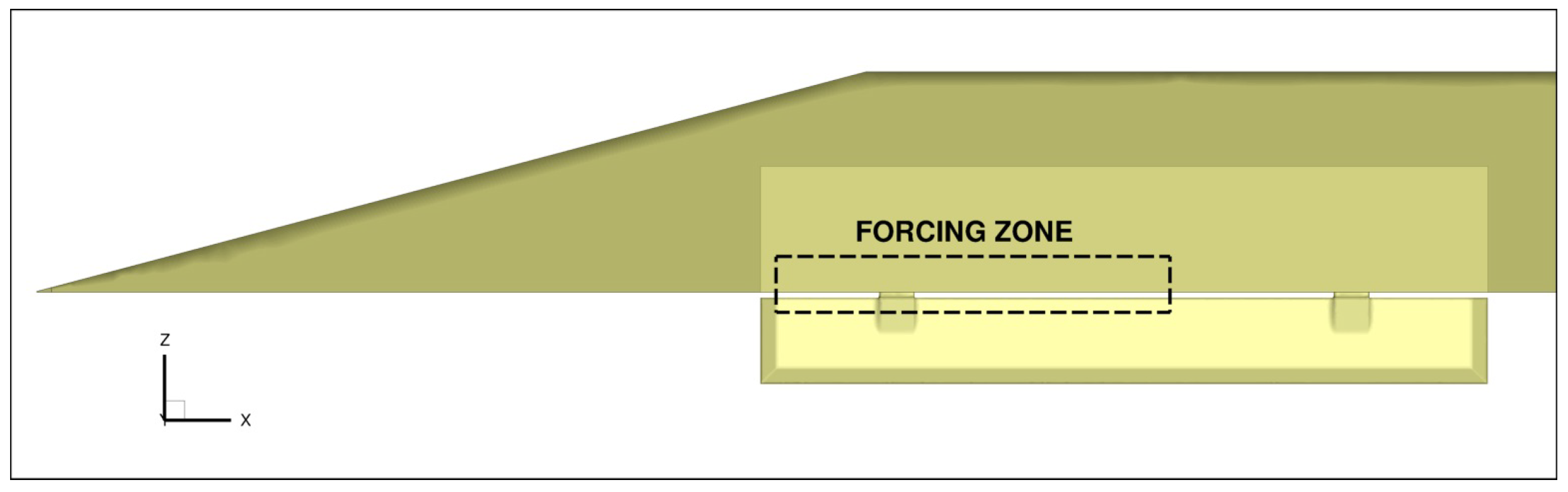
where is the time step size, and is the maximum of grid spacing in the directions. The forcing can be applied to the whole domain (globally) or to a specific region (zonally). In the global prescription of forcing, the SAS model simply damps out the fluctuations in the steady regions. The zonal prescription of forcing does not require additional treatment at the interfaces. Furthermore, the forcing term is only significant in the first few timesteps of the simulation, and its contribution to the momentum equation drops to a negligible value with time as the field contains more resolved structures and an equilibrium between forcing and dissipation develops. As a result, the stability and robustness of the method are similar to the unforced approach. The dimensions of the forcing zone for the present case have been chosen based on the shear-layer prediction from the URANS computations, as shown in Figure 5, roughly extending 50% of the cavity length and 30% of the cavity depth. The highest levels of turbulent kinetic energy in URANS have been identified and enclosed by the forcing zone, as the contribution of the forcing term is directly proportional to the modeled turbulent kinetic energy.
The simulations employ a second-order central scheme for spatial discretization with matrix dissipation schemes. The temporal discretization has been achieved through a dual-time stepping approach, which follows the approach of Jameson [29]. An implicit Euler method is employed for discretizing the time-derivative to generate a sequence of (non-linear) steady-state problems, which make use of the singly diagonally implicit Runge–Kutta method (SDIRK) until a steady state in fictitious pseudo time is reached. The convective Courant–Friedrichs–Lewy number (CFL) has been kept around for the DES-WF and 2.0–3.0 for the SAS variants. The convergence criteria are based on Cauchy convergence control of the variables’ volume-averaged turbulent kinetic energy, maximum eddy viscosity, total vorticity and maximum Mach number with tolerance values of each. Further details regarding the DLR-TAU solver can be found in Galle et al. [30].
3.5. Computational Time Requirements
Table 3 shows the time step size and computational cost reduction relative to the wall-resolved SA-IDDES results (DES-WR) from a previous work [17]. The number of outer iterations per time step has been set to 200, which ensures a reduction in the density residual by two orders of magnitude within a time step. It has been observed that time step size plays a major role in the improvement of computational efficiency within the SAS variants, which allows for a larger time step size due to the underlying RANS nature of the SAS model. The DES-WR and DES-WF simulations are stringent in terms of the time step size, and a higher CFL number leads to misprediction of spectral results.
4. Results and Discussion
This section is organized in three subsections. Section 4.1 will focus on the resonant modes occurring in the cavity for the symmetric flow condition. A comparison of resonant frequencies from the simulation will be shown with the measured values and the theoretical model. The mechanism of each resonant mode has been identified, and a correlation to the flow processes is presented using the results of the DES-WF simulation. Section 4.2 will focus on the performance of the different SAS approaches, namely the SAS-WR, SAS-WF and SAS-F variants, comparing them with experimental and DES-WF simulation data. Additionally, the comparison of RMS pressure, turbulent kinetic energy and von Karman length scales will be illustrated. Upon validation of the SAS approaches, the cavity was simulated under asymmetric flow conditions with the SAS-WR approach to study the directional effect on the resonant modes. These results will be presented and discussed in Section 4.3.
4.1. Prediction of Acoustic Spectrum
During the simulations, unsteady pressure data were collected in the mid-plane of the cavity from locations with a spatial resolution of in the streamwise direction and in the transverse direction for a physical time corresponding to over 500 convective time units (CTU). A fast Fourier transform (FFT) has been performed on the collected data based on Welch’s method to decompose the pressure data into its frequency components. The data have been processed for the FFT analysis using the Hamming window function with the maximum offset length of FFT windows corresponding to the integral time scale computed through the autocorrelation function. The lowest frequency that the simulated data can resolve is kept around 40 Hz for all of the simulations and the experimental data. The first four modal frequencies are listed in Table 4 for the four different simulation strategies, which represent the peaks in the FFT results. The table also shows the theoretically computed modes from the modified Rossiter model (Equation (22)) along with the frequencies of the measured modes [5].
In comparison to the original Rossiter model according to Equation (1), the modified Rossiter model features an additional variable , the adiabatic exponent, derived by assuming the speed of sound in the cavity is equal to the stagnation sonic speed.
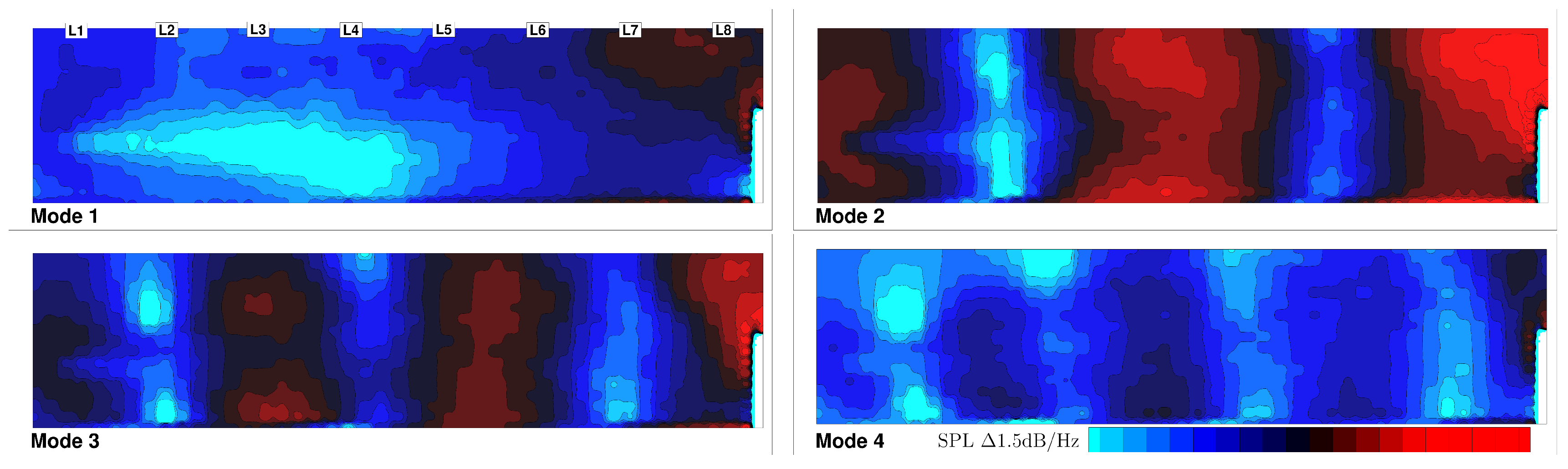
The local amplitudes of the first four resonance modes have been identified on the central plane . They are shown in Figure 6 to visualize the shape of the modes inside the cavity. Rossiter mode 1 has a node in the center of the cavity, anti-nodes on both ends and the front part is significantly overlayed by the shear layer, which suppresses the mode with its broadband frequency ranging between 150–450 Hz. The higher-order Rossiter modes 2, 3 and 4 correspond to the standing waves resulting from the organized vortical structures between the front and rear walls of the cavity. It is also observed that the lip of the cavity in all the modes is overlayed by the shear layer. This result is consistent with the experimental findings by Wagner et al. [9], which explains the relationship between the acoustic tones and flow structure in transonic open cavity flow.
4.2. Performance of the Different SAS Variants
This subsection presents the performance of the different SAS variants with respect to their computational cost, accuracy and robustness. Additionally, some of the flow details of the cavity, such as the turbulent kinetic energy, vorticity magnitude and Reynolds stress, will be presented, as well as the resolution capability of the turbulent structures of the different simulation methods.
4.2.1. Prediction of SPL
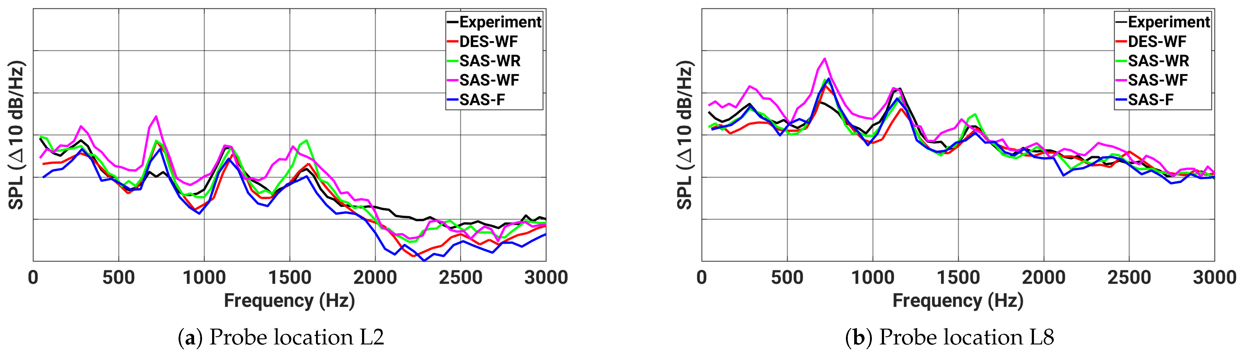
Figure 7 shows the FFT data of the experiment, DES-WF, SAS-WR, SAS-WF and SAS-F simulations for the probe locations L2 and L8. The length of the experimental data made available to this study was s. They have been divided into 40 samples each containing s. Each sample has been processed, and its FFT result is shown in Figure 7 in black color. With a width in the range of 3–4 dB/Hz, the experimental spectrum appears as one block of data, upon which the simulation results are superimposed for validation. This accounts for the effect of the sample length, as the length of the series simulated is s. The Rossiter frequencies are captured extremely well by the DES-WF, SAS-WR and SAS-F simulations, while SAS-WF shows its trend to mispredict the higher modal frequencies. In terms of magnitude, at the probe location L2, the mode 1 is predicted well by the DES-WF, SAS-WR and SAS-F simulations. Mode 2 is over-predicted significantly by the SAS-WF simulation, whereas mode 3 has been captured well by all the simulations. In general, the SAS-WF simulation mispredicts the modal amplitudes but shows the tendency to capture the frequencies as well as the DES-WF and SAS-WR simulations. As the pressure fluctuations are higher near the rear wall, it is considered important to analyze the performance of the simulations at probe location L8. It can be clearly seen that the SPL levels in general are higher at probe location L8 than at L1. Modes 2, 3 and 4 are captured adequately well by SAS-WR, SAS-WF and SAS-F simulations.
To summarize the spectral results, it is observed that the overall behavior of the simulations is extremely good in terms of frequency prediction. However, the magnitudes between the simulations show noticeable differences. In particular, the SAS-WR and SAS-F simulations fit the magnitude levels as good as the DES-WF simulations. The SAS-WF simulation shows some good trends in predicting the spectral distribution with scope for improvement in its magnitude prediction capability, which has been achieved by applying the artificial forcing method (i.e., SAS-F).
4.2.2. Prediction of RMS Pressure
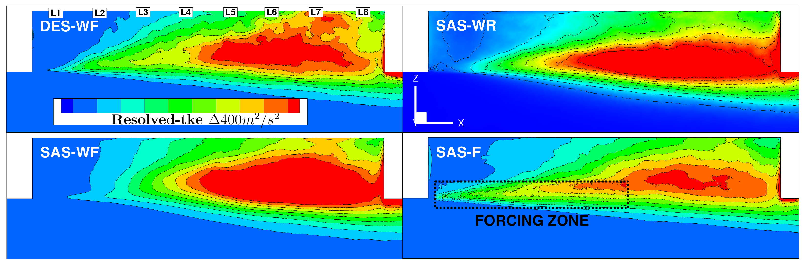
Figure 8 shows the plot of the RMS pressure along the centerline of the cavity ceiling compared with the measured data. In the DES-WF and SAS-F simulations, the predicted RMS pressure fits the experimental data extremely well. In the SAS-WR simulation, the predicted values fit the experimental data within the first third of the cavity length, overpredict in the middle region and capture reasonably well towards the rear portion. In the SAS-WF simulation, the RMS profile follows the trend of DES-WF simulation quite well but overpredicts the values significantly towards the regions of higher pressure RMS. The overpredicting behavior of SAS-WF is also perceivable from the distribution of the resolved turbulent kinetic energy, as shown in Figure 9. The reason for the over-prediction in the SAS-WF simulation is correlated to the delayed production of resolved structures in the shear layer. The activation of the term has been delayed, and, thereby, the shear-layer breakup prediction shows a different behavior than the DES-WF simulation. This delayed prediction of the shear layer has a consequent effect of higher fluctuation intensity over the midsection of the cavity. The shear-layer breakup is considerably delayed compared to both the DES-WF and SAS-WR simulations, and, clearly, this has increased the scale of the fluctuations by a significant margin in the second half of the cavity. In the SAS-F simulation, the forced fluctuations near the lip of the cavity have led to a better prediction capability of the resolved turbulence and, consequently, a better prediction of the RMS pressure is achieved.
4.2.3. Prediction of the Turbulent Flow Field
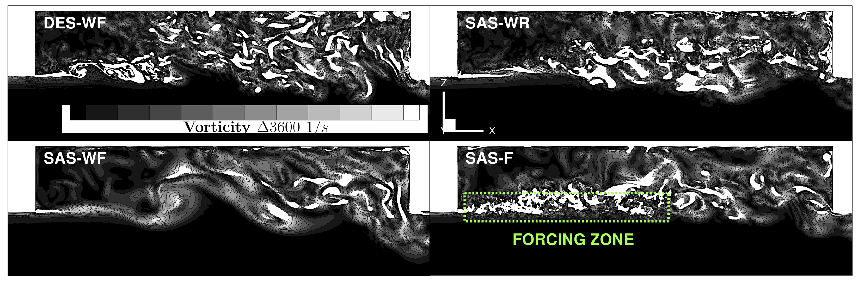
Figure 10 shows the characteristics of open cavity flows captured by all the simulations. Vortices evolve in the shear layer and combine with other turbulent structures as they are convected downstream. Then, they break into smaller structures after impinging on the rear wall of the cavity. In the SAS-F simulation, the shear layer breaks down sooner leading to a vortex shedding process due to the applied artificial forcing technique, an improvement compared to the SAS-WF simulation. The flow structures shed from the front edge and grow in size without abrupt changes outside the forcing zone as they move toward the rear edge. Figure 10 also shows the turbulence-resolving capability inside the cavity from the DES-WF, SAS-WR, SAS-WF and SAS-F simulations. One can see the fine flow field resolution from the DES-WF simulation, which is used as a reference to investigate the capability of the other turbulence models. The SAS variants clearly do not show all of the resolved scales seen in the DES-WF simulation since the scale-resolving ability of the SAS model only becomes active when there are enough fluctuations. Therefore, the structures are resolved in the shear layer and near the rear wall where the shear layer impinges and flows upstream. In the SAS-WF simulation, the fine-scale structures are clearly less pronounced than in the SAS-WR simulation. The wall functions upstream of the wall do not produce resolved structures, and this leads to the visible differences. By enforcing fluctuations in the SAS-F simulation, one can see a better prediction of the vorticity field in the shear layer, which is closer to the DES-WF results.
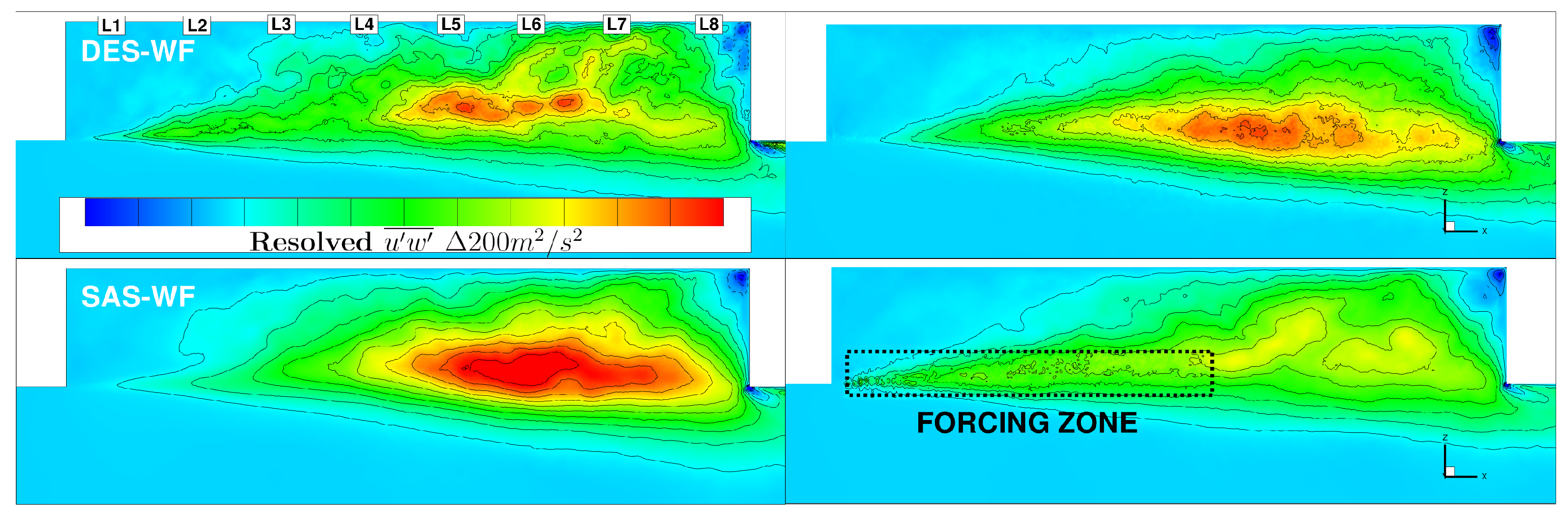
The effect of the forcing term on the resolved turbulence in the SAS approach is also visualized in Figure 11. The profile of the resolved Reynolds stress from the DES-WF simulation appears as a triangular region starting from the lip with the base of the cone at the rear wall. The SAS-WR and SAS-WF simulations show the apex of the triangle delayed and extending less upstream than in the DES-WF simulation. Activation of the forced fluctuation results in converting the model into resolved turbulent kinetic energy, and, eventually, this aids in predicting the resolved fluctuations near the lip of the cavity as well as the DES-WF simulation. Moreover, as a consequence of this process, one can see the profiles of the Reynolds stress components downstream of the forcing zone closer to those of the DES-WF simulation.
4.2.4. Prediction of von Karman Length Scale and Boundary Layer Thicknesses
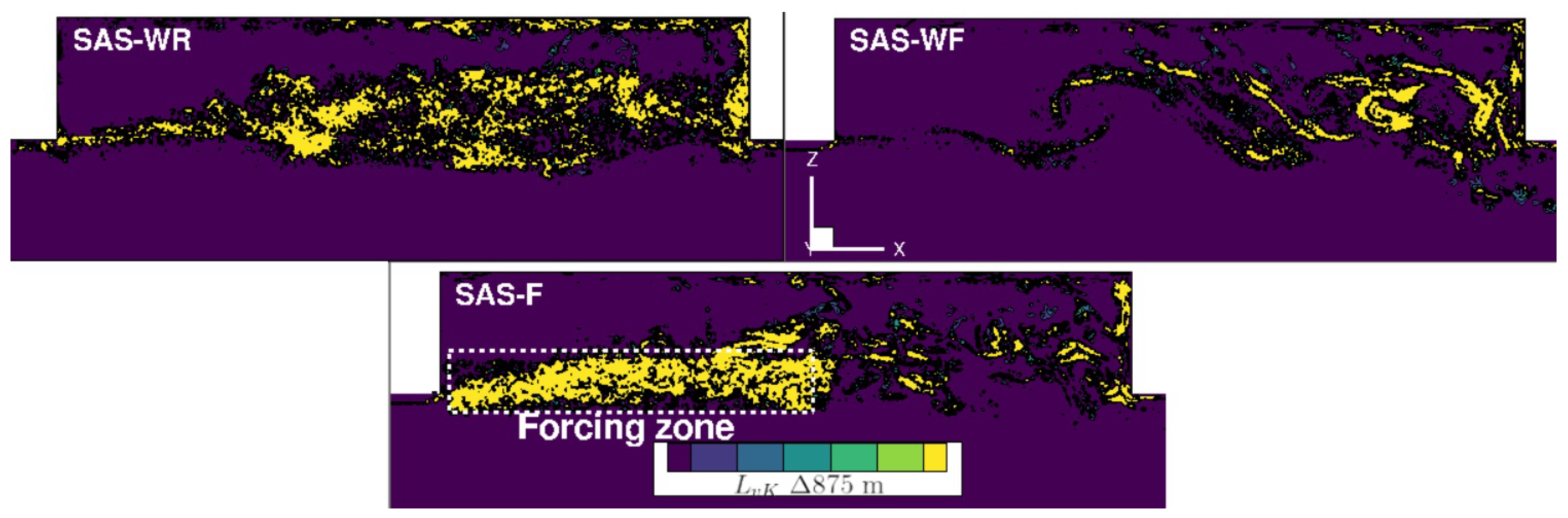
For further investigation of the differences between the SAS simulations, the distribution of the von Karman length scale has been investigated. The only difference between the SAS-WR and SAS-WF (or SAS-F) meshes is the number of prism layers close to the wall. The SAS-WR mesh has 35 prism layers with a value less than for the first element, whereas the SAS-WF mesh has 10 prism layers with a value greater than 100. It is noteworthy to investigate the von Karman length scale, , present in the different SAS variants (see Figure 12). The von Karman length scale represents a key element in triggering the model to allow the generation of resolved turbulence in SAS simulations. As seen in Figure 12, is produced strongly over a larger region in the SAS-WR simulation, whereas, in the SAS-WF simulation, the region of presence is limited. The largest difference appears near the upstream wall of the cavity. The usage of wall functions has rendered the SAS model to operate in URANS mode near the upstream wall of the cavity, which has led to the differences in the resolved structures inside the cavity. By contrast, the SAS-F model operates in resolving mode close to the front edge of the cavity due to forcing-induced structures, which leads to a better prediction of the shear-layer growth and its breakdown.
The flat-plate boundary layer region at a distance upstream of the cavity has been analyzed, and the shape factor (i.e., the ratio of displacement to momentum thickness) has been determined as in the case of DES-WF simulation, with the local Reynolds number, . The thickness for the DES-WF reference case has been found to be , which coincides with the SAS-WR prediction, with representing the distance of the local point from the leading edge of the cavity rig. Relative to the DES-WF case, there is an overprediction of 5– in the displacement and momentum thicknesses in the SAS-WR simulation. The SAS-WF and SAS-F simulations predicted more in the thicknesses, both showing deviations of the shape factor as low as .
4.3. Impact of Asymmetric Flow Conditions
Upon successful validation of the SAS approaches (see Section 4.2), a case of the sideslip study with was simulated in order to study the effect of asymmetric flow conditions on the presence of resonant modes. This subsection will show the modulation effect of the sideslip angles on the measured spectral modes, including the reliability of the SAS method under different flow conditions and the investigation of lateral wall effects on the cavity flow features. The flow under sideslip conditions naturally involves more turbulent fluctuations than symmetric flow conditions, which aid in the activation of the SAS mode. Therefore, the SAS-WR approach has been found to be a sufficient method for the considered case. Since the forcing zone approach does not require any additional treatment at the interface, one could also use the SAS-F method for sideslip conditions without special requirements for the case.
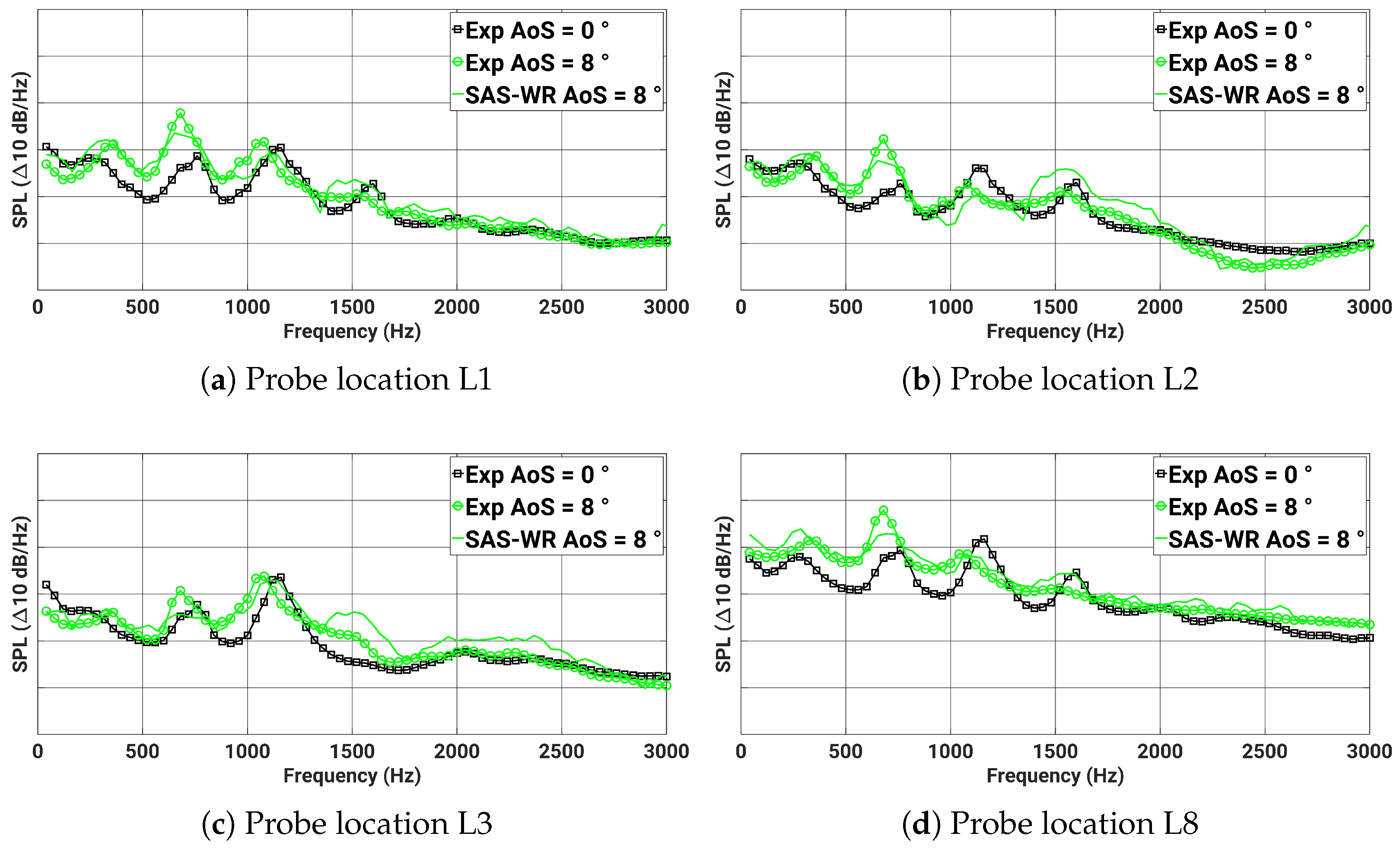
Figure 13 shows the FFT spectrum of four probe locations along the cavity ceiling. The general shape of the spectra occurring in all the probe locations has been predicted to be in good agreement with the experimental data. The relative magnitudes between the modes also have been predicted well. Mode 2 has been slightly under-predicted by the simulation for all the probe locations. As the sideslip angle increases, the frequencies at which the resonant modes occur decrease, and the modal amplitudes increase, which is well captured by the simulation results. It has been shown in Section 4.2 that using wall functions leads to stronger vortices in the shear layer and subsequent overprediction of spectral amplitudes, although the spectral frequencies fit the experimental data well. This suggests that the resonant frequencies are correlated to the interaction time scale between the aerodynamic disturbances from the shear layer and upstream-traveling acoustic waves. This interaction time scale is a direct consequence of the cavity length, as seen in the Rossiter model for frequency estimation (Equation (1)). As the sideslip angle increases, the interaction time scale between them also increases due to the skewed shear-layer flow inside the cavity, and the frequencies at which the peaks occur decrease as a result.
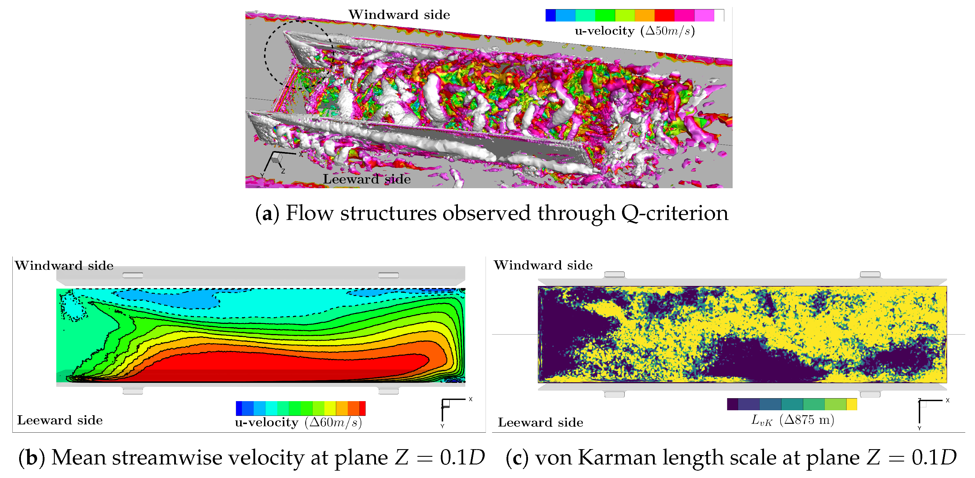
In addition to the flow structures shed from the front edge of the cavity, there are additional structures from the edge of the windward-side door added to the shear layer marked by the dashed circle in Figure 14a. The structures merge, and they enlarge in size while being convected in the shear layer before impinging on the end of the leeward-side door and the rear wall of the cavity. On impingement, the flow is redirected spanwise, flows upstream and interacts with the oncoming shear layer. The spanwise recirculation can be seen with the negative u-velocity marked with dotted lines in Figure 14b. The activation of the resolving mode in the model is presented in Figure 14c, which shows the distribution of the local von Karman length scale at the same instant in time as in Figure 14b. In the regions of higher values, the eddy viscosity is reduced, and, subsequently, the turbulence is resolved down to the underlying cell size.
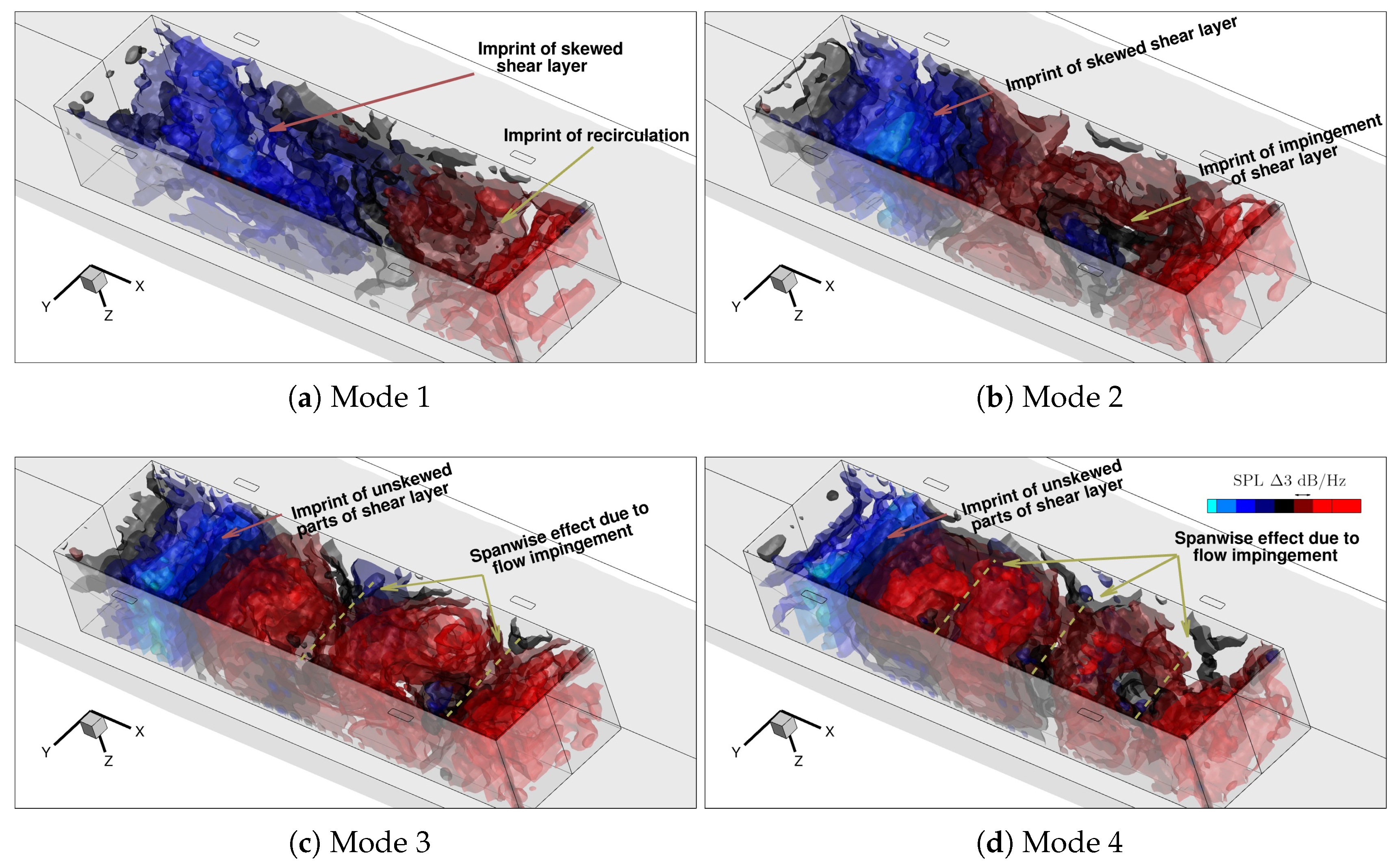
The amplitudes of the first four resonance modes were determined and their isosurfaces are shown in Figure 15 to identify the nature of the modes. It is observed that there is a dominant longitudinal propagation of waves inside the cavity. In addition, there is a contribution from spanwise propagating waves in the higher modes. Basically, mode 1 is governed by the bulk flow processes in the cavity, namely the shear layer and the recirculation process. It is to be noted that the shear layer is skewed due to the presence of the windward door. The resonance between these two large-scale mechanisms correlates to mode 1 in the cavity. The contribution of skewed components of the shear layer decreases as the mode number increases. Higher modes 2, 3 and 4 comprise gradually less skewed shear-layer components that encounter the leeward wall, which then leads to spanwise standing waves. Furthermore, in the streamwise direction, more nodes with shorter wavelengths exist with an increasing mode number or the wavenumber of the modes becomes smaller with an increasing mode number. To summarize, mode 1 encompasses the large-scale skewed dynamics of the shear layer, whereas the higher modes correlate to the shedding flow structures from the unskewed parts of shear layer and have a contribution from spanwise components initiated by the flow interaction on the leeward side. This contribution results in an increase in modal amplitudes for asymmetric flow conditions.
5. Conclusions and Outlook
In this study, an open cavity configuration with sidewise doors has been studied numerically with different simulation methodologies, such as DES with wall functions (DES-WF) and SAS with resolved walls (SAS-WR), wall functions (SAS-WF) and an artificial forcing method (SAS-F) for the transonic flow conditions of and . The correlation of the Rossiter modes with the flow processes has been identified in detail through the FFT of the DES-WF simulation results. It has been proven that all the simulation methodologies can capture the Rossiter frequencies well with a certain overprediction of spectral magnitudes by the SAS-WF simulation. The reason for the overprediction has been investigated and identified as being caused by the lack of resolved turbulence inside the cavity. The commonalities and differences between the individual SAS simulations were revealed and outlined in this article based on the von Karman length scale and vorticity fields. To overcome the problem of the URANS regions in the SAS-WF simulation, the artificial forcing technique has been employed. In terms of computational requirements, the DES-WF and SAS-WR simulations are estimated to be around and cheaper than the wall-resolved DES simulation, respectively, whereas the SAS-WF and SAS-F simulations are almost twice as fast as the SAS-WR simulation. Furthermore, the mechanism behind the Rossiter modes under sideslip conditions and their modulations has been discussed. It has been shown using isosurfaces of the modes that a significantly higher interference of waves occurs in a highly three-dimensional manner between the walls of the cavity. Mode 1 is a result of the skewed shear-layer dynamics, and higher modes contain less skewed shear-layer contents along with spanwise reflecting waves. In addition to the streamwise waves, a significant wave interference takes place in the spanwise direction due to the impingement of flow on the leeward door. It is beyond the scope of this work to show the performance of SAS-F for sideslip conditions, however, it would be worth investigating its performance under skewed flow behavior with respect to the front edge of the cavity. Moreover, additional flow cases with asymmetric flow conditions would be of interest to reveal more significant 3D effects in the cavity.
Author Contributions
Conceptualization, K.R., E.T. and M.K.; methodology, K.R., E.T. and M.K.; software, K.R.; validation, K.R.; formal analysis, K.R.; investigation, K.R.; data curation, K.R.; writing—original draft preparation, K.R.; writing—review and editing, K.R., E.T. and M.K.; visualization, K.R.; supervision, E.T. and M.K.; project administration, E.T. and M.K.; funding acquisition, E.T. and M.K. All authors have read and agreed to the published version of the manuscript.
Funding
This work has been carried out with financial support from Airbus Defence and Space (ADS) under the project “Analysis of Unsteady Effects in Fighter Aircraft Aerodynamics”, which is gratefully acknowledged. Furthermore, the experimental survey has been carried out by ADS and made available to this study for the validation of numerical results.
Data Availability Statement
The data that support the findings of this study are available from the authors upon reasonable request.
Acknowledgments
The authors would like to acknowledge the German Aerospace Center (DLR) for providing the TAU code and Ennova Technologies, Inc., for the meshing software. The authors would also like to acknowledge the Gauss Centre for Supercomputing for making the required computing hours available to this study (Account number pn29xa).
Conflicts of Interest
The authors declare no conflict of interest.
References
- Krishnamurty, K. Acoustic Radiation from Two-Dimensional Rectangular Cutouts in Aerodynamic Surfaces; NASA Technical Note 3487; NASA: Washington, DC, USA, 1955; p. 36.
- Rossiter, J. Wind Tunnel Experiments on the Flow over Rectangular Cavities at Subsonic and Transonic Speeds; Technical report; Her Majesty’s Stationery Office: London, UK, 1964.
- Dix, R.E.; Bauer, R.C. Experimental and Theoretical Study of Cavity Acoustics; Technical report; Sverdrup Technology, Inc./AEDC Group: Allen Park, MI, USA, 1997. [Google Scholar]
- Woo, C.H.; Kim, J.S.; Lee, K.H. Three-dimensional effects of supersonic cavity flow due to the variation of cavity aspect and width ratios. J. Mech. Sci. Technol. 2008, 22, 590–598. [Google Scholar] [CrossRef]
- Heller, H.H.; Holmes, D.G.; Covert, E.E. Flow-induced pressure oscillations in shallow cavities. J. Sound Vib. 1971, 18, 545–553. [Google Scholar] [CrossRef]
- Henderson, J.; Badcock, K.; Richards, B.E. Subsonic and transonic transitional cavity flows. In Proceedings of the 6th Aeroacoustics Conference and Exhibit, Lahaina, HI, USA, 12–14 June 2000. [Google Scholar] [CrossRef]
- Lawson, S.J.; Barakos, G.N. Review of numerical simulations for high-speed, turbulent cavity flows. Prog. Aerosp. Sci. 2011, 47, 186–216. [Google Scholar] [CrossRef]
- Gloerfelt, X.; Bogey, C.; Bailly, C. Numerical Evidence of Mode Switching in the Flow-Induced Oscillations by a Cavity. Int. J. Aeroacoust. 2003, 2, 193–217. [Google Scholar] [CrossRef]
- Wagner, J.L.; Casper, K.M.; Beresh, S.J.; Arunajatesan, S.; Henfling, J.F.; Spillers, R.W.; Pruett, B.O. Relationship between acoustic tones and flow structure in transonic cavity flow. In Proceedings of the 45th AIAA Fluid Dynamics Conference, Dallas, TX, USA, 22–26 June 2015; pp. 1–16. [Google Scholar]
- Rowley, C.W.; Colonius, T.; Basu, A.J. On self-sustained oscillations in two-dimensional compressible flow over rectangular cavities. J. Fluid Mech. 2002, 455, 315–346. [Google Scholar] [CrossRef]
- Chang, K.; Constantinescu, G.; Park, S. Assessment of predictive capabilities of detached eddy simulation to simulate flow and mass transport past open cavities. J. Fluids Eng. Trans. ASME 2007, 129, 1372–1383. [Google Scholar] [CrossRef]
- Nayyar, P.; Barakos, G.N.; Badcock, K.J. Numerical study of transonic cavity flows using large-eddy and detached-eddy simulation. Aeronaut. J. 2007, 111, 153–164. [Google Scholar] [CrossRef]
- Stanek, M.J.; Visbal, M.R.; Rizzetta, D.P.; Rubin, S.G.; Khosla, P.K. On a mechanism of stabilizing turbulent free shear layers in cavity flows. Comput. Fluids 2007, 36, 1621–1637. [Google Scholar] [CrossRef]
- Wang, H.; Sun, M.; Qin, N.; Wu, H.; Wang, Z. Characteristics of oscillations in supersonic open cavity flows. Flow Turbul. Combust. 2013, 90, 121–142. [Google Scholar] [CrossRef]
- Girimaji, S.; Werner, H.; Peng, S.; Schwamborn, D. Progress in hybrid RANS-LES modelling. In Proceedings of the 5th Symposium on Hybrid RANS-LES Methods, College Station, TX, USA, 19–21 March 2014; pp. 19–21. [Google Scholar]
- Menter, F.R.; Garbaruk, A.; Smirnov, P.; Cokljat, D.; Mathey, F. Scale-adaptive simulation with artificial forcing. Notes Numer. Fluid Mech. Multidiscip. Des. 2010, 111, 235–246. [Google Scholar] [CrossRef]
- Rajkumar, K.; Tangermann, E.; Klein, M.; Ketterl, S.; Winkler, A. DES of Weapon Bay in Fighter Aircraft Under High-Subsonic and Supersonic Conditions. Notes Numer. Fluid Mech. Multidiscip. Des. 2021, 151, 656–665. [Google Scholar] [CrossRef]
- Mayer, F.; Mancini, S.; Kolb, A. Experimental investigation of installation effects on the aeroacoustic behaviour of rectangular cavities at high subsonic and supersonic speed. In Proceedings of the Deutscher Luft- und Raumfahrtkongress, Online, 1–3 September 2020. [Google Scholar]
- Langer, S.; Schwöppe, A.; Kroll, N. The DLR flow solver TAU—Status and recent algorithmic developments. In Proceedings of the 52nd Aerospace Sciences Meeting, National Harbor, MA, USA, 13–17 January 2014. [Google Scholar] [CrossRef]
- Rajkumar, K.; Tangermann, E.; Klein, M.; Ketterl, S.; Winkler, A. Time-efficient simulations of fighter aircraft weapon bay. CEAS Aeronaut. J. 2023, 14, 91–102. [Google Scholar] [CrossRef]
- Rajkumar, K.; Radtke, J.; Tangermann, E.; Klein, M. Open cavity simulations under sideslip conditions. In Proceedings of the Congress of the International Council of the Aeronautical Sciences, Stockholm, Sweden, 4–9 September 2022. [Google Scholar]
- Rajkumar, K.; Tangermann, E.; Klein, M. Towards high fidelity weapon bay simulations at affordable computational cost. In Proceedings of the AIAA Aviation Forum, Chicago, IL, USA, 27 June–1 July 2022. [Google Scholar]
- Kolmogorov, A. The Local Structure of Turbulence in Incompressible Viscous Fluid for Very Large Reynolds Numbers. Dokl. Akad. Nauk. SSSR 1941, 30, 301–304. [Google Scholar]
- Swanson, R.C.; Radespiel, R.; Turkel, E. On Some Numerical Dissipation Schemes. J. Comput. Phys. 1998, 147, 518–544. [Google Scholar] [CrossRef] [Green Version]
- Allmaras, S.R.; Johnson, F.T.; Spalart, P.R. Modications and Clarications for the Implementation of the Spalart-Allmaras Turbulence Model. In Proceedings of the Seventh International Conference on Computational Fluid Dynamics, Waimea, HI, USA, 9–13 July 2012; pp. 9–13. [Google Scholar]
- Spalart, P.R.; Allmaras, S.R. A one-equation turbulence model for aerodynamic flows. In Proceedings of the 30th Aerospace Sciences Meeting and Exhibit, Reno, NV, USA, 6–9 January 1992; pp. 5–21. [Google Scholar] [CrossRef]
- Menter, F.R. Two-equation eddy-viscosity turbulence models for engineering applications. AIAA J. 1994, 32, 1598–1605. [Google Scholar] [CrossRef] [Green Version]
- Kraichnan, R.H. Diffusion by a random velocity field. Phys. Fluids 1970, 13, 22–31. [Google Scholar] [CrossRef]
- Jameson, A.; Schmidt, W.; Turkel, E. Numerical solution of the euler equations by finite volume methods using Runge Kutta time stepping schemes. In Proceedings of the 14th Fluid and Plasma Dynamics Conference, Palo Alto, CA, USA, 23–25 June 1921; American Institute of Aeronautics and Astronautics (AIAA): Reston, VA, USA, 1981; Volume 6. [Google Scholar] [CrossRef] [Green Version]
- Galle, M.; Gerhold, T.; Evans, J. Parallel Computation of Turbulent Flows around Complex Geometries on Hybrid Grids with the DLR-Tau Code. In Proceedings of the 11th Parallel CFD Conference, Orlando, FL, USA, 6–9 July 1999. [Google Scholar]
Figure 1.
Weapon bay model with the position of probes [22].
Figure 1.
Weapon bay model with the position of probes [22].

Figure 2.
Mesh distribution for the DES-WF simulation.

Figure 3.
Mesh convergence study based on energy spectra.

Figure 4.
distance over the cavity walls in the DES-WF simulation at an instant of time [22].
Figure 4.
distance over the cavity walls in the DES-WF simulation at an instant of time [22].

Figure 5.
Forcing zone in SAS-F simulation [22].
Figure 5.
Forcing zone in SAS-F simulation [22].

Figure 6.
SPL of the Rossiter modes predicted by the DES-WF simulation.

Figure 7.
Comparion of SPL predicted by the DES-WF, SAS-WR, SAS-WF and SAS-F simulations.

Figure 8.
Comparison of the RMS pressure predicted by the DES-WF, SAS-WR, SAS-WF and SAS-F simulations [22].
Figure 8.
Comparison of the RMS pressure predicted by the DES-WF, SAS-WR, SAS-WF and SAS-F simulations [22].

Figure 9.
Resolved turbulent kinetic energy in the DES-WF, SAS-WR, SAS-WF and SAS-F simulations [22].
Figure 9.
Resolved turbulent kinetic energy in the DES-WF, SAS-WR, SAS-WF and SAS-F simulations [22].

Figure 10.
Instantaneous vorticity magnitude in the DES-WF, SAS-WR, SAS-WF and SAS-F simulations [22].
Figure 10.
Instantaneous vorticity magnitude in the DES-WF, SAS-WR, SAS-WF and SAS-F simulations [22].

Figure 11.
Distribution of the Reynolds stress in the DES-WF, SAS-WR, SAS-WF and SAS-F simulations [22].
Figure 11.
Distribution of the Reynolds stress in the DES-WF, SAS-WR, SAS-WF and SAS-F simulations [22].

Figure 12.
Prediction of the von Karman Length scale, in the SAS-WR, SAS-WF and SAS-F simulations [22].
Figure 12.
Prediction of the von Karman Length scale, in the SAS-WR, SAS-WF and SAS-F simulations [22].

Figure 13.
SPL of probe locations at .

Figure 14.
Flow visualization at .

Figure 15.
Visualization of modes at .


Table 1.
Details of Mesh A, B and C for mesh refinement study in SAS-WR.
| Mesh A | Mesh B | Mesh C | |
|---|---|---|---|
| Number of mesh nodes | |||
| of the first element | |||
| Number of prism cells | 35 | 35 | 35 |
| Resolution in Regions I and II |
Table 2.
Details of the meshes applied for the productive simulation runs.
| DES-WF | SAS-WR | SAS-WF | SAS-F | |
|---|---|---|---|---|
| Number of mesh nodes | ||||
| of the first element | >100.0 | <1.0 | >100.0 | >100.0 |
| Number of prism cells | 10 | 35 | 10 | 10 |
| Resolution in Region I | ||||
| Resolution in Region II | - | - | - |
Table 3.
Computational requirements relative to DES-WR.
| DES-WF | SAS-WR | SAS-WF | SAS-F | |
|---|---|---|---|---|
| Number of outer iterations per time step | 200 | 200 | 200 | 200 |
| Physical time step size | 1.5 | 7 | 7 | 7 |
| Drop in density residual within one time step | ∼O () | ∼O () | ∼O () | ∼O () |
| Comp. cost reduction relative to DES-WR |
Table 4.
Prediction of Rossiter frequencies by modified Rossiter model (Equation (22)), experiment and the simulations.
Table 4.
Prediction of Rossiter frequencies by modified Rossiter model (Equation (22)), experiment and the simulations.
| Mode | Theory | Exp. | DES-WF | SAS-WR | SAS-WF | SAS-F |
|---|---|---|---|---|---|---|
| 1 | 263 | 272 | 278 | 279 | 280 | 285 |
| 2 | 670 | 755 | 722 | 719 | 719 | 743 |
| 3 | 1076 | 1160 | 1167 | 1159 | 1159 | 1143 |
| 4 | 1484 | 1600 | 1611 | 1599 | 1519 | 1600 |
Disclaimer/Publisher’s Note: The statements, opinions and data contained in all publications are solely those of the individual author(s) and contributor(s) and not of MDPI and/or the editor(s). MDPI and/or the editor(s) disclaim responsibility for any injury to people or property resulting from any ideas, methods, instructions or products referred to in the content. |
© 2023 by the authors. Licensee MDPI, Basel, Switzerland. This article is an open access article distributed under the terms and conditions of the Creative Commons Attribution (CC BY) license (https://creativecommons.org/licenses/by/4.0/).
Share and Cite
MDPI and ACS Style
Rajkumar, K.; Tangermann, E.; Klein, M. Efficient Scale-Resolving Simulations of Open Cavity Flows for Straight and Sideslip Conditions. Fluids 2023, 8, 227. https://0-doi-org.brum.beds.ac.uk/10.3390/fluids8080227
AMA Style
Rajkumar K, Tangermann E, Klein M. Efficient Scale-Resolving Simulations of Open Cavity Flows for Straight and Sideslip Conditions. Fluids. 2023; 8(8):227. https://0-doi-org.brum.beds.ac.uk/10.3390/fluids8080227
Chicago/Turabian StyleRajkumar, Karthick, Eike Tangermann, and Markus Klein. 2023. "Efficient Scale-Resolving Simulations of Open Cavity Flows for Straight and Sideslip Conditions" Fluids 8, no. 8: 227. https://0-doi-org.brum.beds.ac.uk/10.3390/fluids8080227