Influence of Car Configurator Webpage Data from Automotive Manufacturers on Car Sales by Means of Correlation and Forecasting

Abstract

A methodology to prove the influence of car configurator webpage data for automotive manufacturers is developed across this research. Firstly, the correlation between online data and sales is measured. Afterward, car variant sales are predicted using a set of forecasting techniques divided into univariate and multivariate ones. Finally, weekly color mix sales based on these techniques are built and compared. Results show that users visit car configurator webpages 1 to 6 months before the purchase date. Additionally, car variants predictions and weekly color mix sales derived from multivariate techniques, i.e., using car configurator data as external input, provide improvement up to 25 points in the assessment metric.

1. Introduction

The manufacturing sector confronts one big challenge: matching product customization to satisfy the largest number of customers. Their attempt to solve this problem consists of offering a large portfolio, so customers can choose from it. Nevertheless, this solution implies that production, inventory, and logistics should be adapted to the demand, as far as companies continue working with the build-to-stock (BTS) strategy. In this framework, demand forecasting plays a relevant role.

Capturing in advance the requests of potential customers drives inventory and production optimization. In the modern era, these requests can be collected from the Internet. They exist in the form of search queries, activity on social media, etc. In the literature, there are examples of economical sectors where this information source was an input of a demand forecasting system, as in the cases of e-commerce [1], the entertainment sector [2], the food industry [3], tourism [4], and the editorial sector [5].

The above examples make reference to low-value purchases, customers are not highly involved, and there are no relevant differences between brands. Products or services with the opposite characteristics are defined as high-implication purchases. One of the economical sectors that fulfill these criteria is the real estate market. This area is not ignorant about the use of Internet data. Several authors in the literature have explored the utility of the Internet as an external source to capture the customers’ requests. References [6,7,8,9,10,11] are proof of this.

However, in this note we present another economical sector of high-implication purchases: the car market. Automotive original equipment manufacturers (OEMs) face the same difficulties as a BTS system, as it is extensively explained in works [12,13,14,15,16]. The main difference with respect to other sectors is that they are in possession of a unique tool to acquire customers’ demand. They do not depend on third parties such as Internet browsers or social media. Specifically, we are mentioning the brand’s car configurator (CC) webpage. It is a service where potential customers can customize their wished car. Additionally, they can compare different options and car attributes, and get a first acquisition price. These are the reasons that drive us to propose the following research question: Is the brand’s car configurator webpage data a reliable source to capture in advance customers’ demand?

This research proposes a manner of measuring the reliability of CC data. It can be easily extended to all automotive OEMs with this online service. We compare the real weekly color mix sales vs. forecast ones. The latter are built using a set of forecasting machine learning (ML) algorithms and statistical procedures based on past sales with or without CC data. Weekly color mix sales are the set of weights each car variant (car model plus color) has over the total weekly sales volume.

Our results show that forecasting techniques assembled with CC data imply an improvement up to nearly 8 points at the car-model and time-chunk level. With respect to weekly color mix sales, the accuracy of techniques assembled with CC data performs up to 25 points better than those based exclusively on past sales. In order to achieve these numbers, firstly it has been analyzed the correlation between sales and CC data. It is a previous step to prove the influence of CC data over future sales. It has been discovered that the period of maximum correlation occurs between 1 and 6 months before the purchase.

We focus on the color feature of a vehicle because it can be changed roughly until the last moment of the production flow. Additionally, the change is not limited by any physical restrictions, such as the availability of a spare component. This flexibility is optimal for a tense supply chain such as the one in the automotive industry. Moreover, recent surveys show that color is a key factor for 88% of car buyers [17].

The article is structured in the following way. Firstly, in Section 2, we present related works for the research topic. Hence, Section 3 describes the dataset provided by the automotive OEM source. Next, the methodology and results of the research are in Section 4 and Section 5, respectively. The discussion takes place in Section 6. Finally, Section 7 provides conclusions gained and future research paths.

2. Related Works

This section scouts the academic efforts to manage Internet data as a reliable source for forecasting. Examples in different economical sectors are presented and the automotive market is exposed. Finally, research gaps and authors’ proposals are described.

2.1. State-of-the Art Review

Nowadays, academia vastly explores the use of Internet data as a manner to gain customers’ requests. However, there are concerns in the industry about the trustworthiness of online information. Past sales and the intuition of the experts are the fundamentals of current BTS systems.

That is why it is necessary to comprehend the relationship that may exist between sales and Internet data. The tool to prove this concept is the Pearson correlation coefficient (PCC) [18]. This statistical development requires dependency between the distributions and positive standard deviations. Other tools to examine this magnitude are Spearman’s rank correlation [19] and mutual information [20]. However, we decide to proceed with PCC given its popularity and efficiency in problems of the same nature. The authors of [21] use PCC to rank the inputs variables for the Bayesian network predictor of traffic flow. Similarly, paper [22] maximizes the relevancy and minimizes the redundancy criterion based on PCC for the electricity load forecasting model. Another example is found in reference [23]. They propose an extension of the PCC measure for cases where similarity does not exist between users of a recommender system.

Previous works prove the validity of PCC in forecast systems. However, the relationship between Internet data and sales has not been discussed yet. Paper [24] uses search query volume to forecast the opening weekend box-office revenue for feature films, first-month sales of video games, and the rank of songs on the Billboard Hot 100 chart. They show that customers’ online activity represents future behavior days or even weeks in advance. In the stock market, reference [25] shows that daily trading volumes of stocks traded in NASDAQ-100 are correlated with daily volumes of queries related to the same stocks. In particular, query volumes anticipate in many cases peaks of trading by one day or more. Lastly, the Chinese retail sector and Internet data are treated in [26]. They explore the correlation between consumers’ web search behavior and purchase behavior theoretically.

Therefore, we progress an investigation of how the literature has dealt with Internet data in relation to the automotive market. Commonly, this information has been treated from two points of view: data acquired from social media or data coming from Internet search queries.

As an example of social media data, reference [27] focuses on the sentiment analysis of social media and car review online sites, together with average monthly sales, to perform sales prediction before and after the launch of the vehicle. Another case is found in [28], where they performed a comparison of the outputs given by different multivariate regression models and time series models which combines monthly total vehicle sales in the USA together with sentiment scores from Twitter, stock market values, or a mix of both external information.

On the other side, an early example from 2009 is found in [29]; they include Google Trends in a logarithmic autoregressive model to predict vehicle sales. Another interesting case is paper [30]; they use a novelty Bass diffusion model that includes customer Internet search behavior with the purpose of explaining product diffusion, gaining significant information in about 84% of the samples, and help to predict new product diffusion. Publication [31] develops a backward induction approach to identify keywords that are frequently used by search engine users of the automotive market and, together with economic variables, the authors can predict monthly car sales. Research done in [32] focuses on the German market and performed long-term prediction by adding the information extracted from macroeconomic variables and online search queries. Similarly, reference [33] does a similar exercise on the car markets of Germany and the UK. They prove that online search data are correlated across products, but to different extent. Hence, they develop a model linking search motives to observable search data and sales.

Nevertheless, there are examples that take advantage of both social media and search queries, such as paper [34]. They compare the outputs of the linear regression model of about a half million posts on social media for eleven car models in the Netherlands against the predictions derived from Google Trends. Paper [35] customizes the typical Bass predictive model of car sales forecasting by adding user-generated Internet information, search traffic, and macroeconomic data to get more accurate predictions. In every previous case, the addition of Internet data outperformed the results of the rest of the models.

2.2. Research Gap

To sum up, Internet data has proved its validity for many years as a powerful predictor in different economic areas. As a general division, Internet data are used in the form of search queries or data collected from social media. We have explored retail, entertainment, real estate, etc., but we focused our attention on the automotive market.

However, we did not find evidence of Internet data in the form of visits to the automotive brand’s CC webpage. The characteristics of the tool clearly distinguish it from search queries or social media. It may have inconsistencies or unknowns due to its own nature. We can assume that users accessing this tool are willing to purchase a vehicle. Nevertheless, it is difficult to distinguish between a visitor and a person with real purchase interest. Actually, we mention a free service given by the manufacturer to the audience to capture its interest. However, it does not demand any kind of commitment from the latter. Hence, the conversion rate is not as straightforward as we could figure out.

Therefore, we propose a path to define the influence of CC data on car sales. Firstly, we will work exclusively with CC data from users who completed the full journey. Following, we measure the correlation between sales and CC data at different granularity and temporal ranges. Afterward, we propose the last verification. Comparison between real weekly color mix sales and forecast ones is carried on. The last-mentioned are based on past sales with or without CC data. It is a new strategy, extensive to all automotive OEMs, to prove the impact of CC data on future sales. Afterward, this data source can leverage other demand prediction approaches with more traditional features, such as financial, press, etc. widely explored in the literature.

3. Dataset Description

This section briefly describes the history of the OEM company that provides the data and the characteristics of the cars they produce, the timespan of the datasets, and some main descriptive values of the sales record and CC visits history in terms of car variants.

3.1. Automotive OEM and Car Model Description

SEAT is a Spanish car manufacturer belonging to the Volkswagen group since 1986 together with other brands such as Audi, Skoda, and Porsche, among others. It is present in 75 countries and in 2019 it manufactured worldwide more than 574,000 cars [36], being the best year of the company. It is focused on the market segment of mass population cars, although since 2018 a new brand called CUPRA was born as a subsidiary of SEAT specialized in high-performance motorsports. From all the catalog of cars under the brand SEAT, only those ones manufactured in the headquarter facilities of the company are the object of study, i.e., Model A and Model B, made from the same platform, and models Model C and Model D, derived from the same architecture.

Table 1. Car segments and quantity of colors available along the entire time span for each car model.

Car Model	Car Segment	Number of Colors
Model A	B	46
Model B	B	12
Model C	C	14
Model D	C	14

describes the car segment and quantity of colors available for each car model along the entire time span of the dataset.

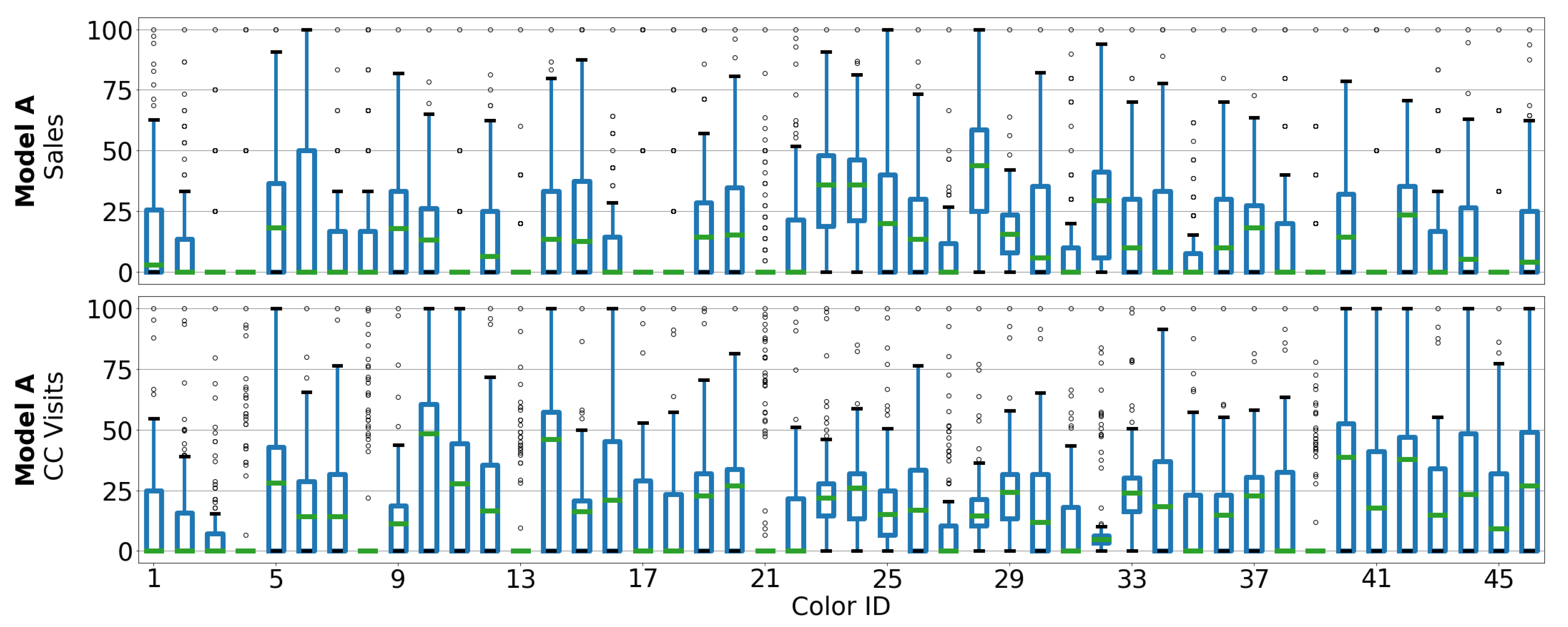
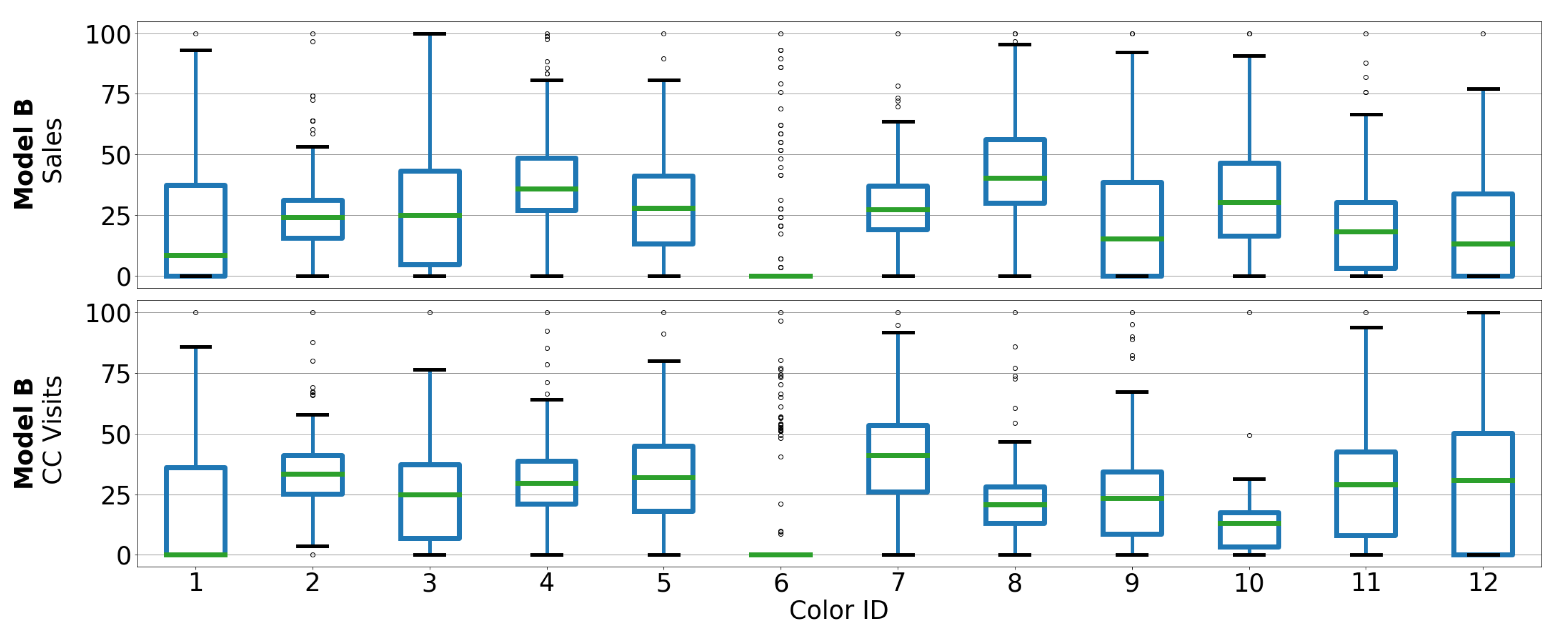
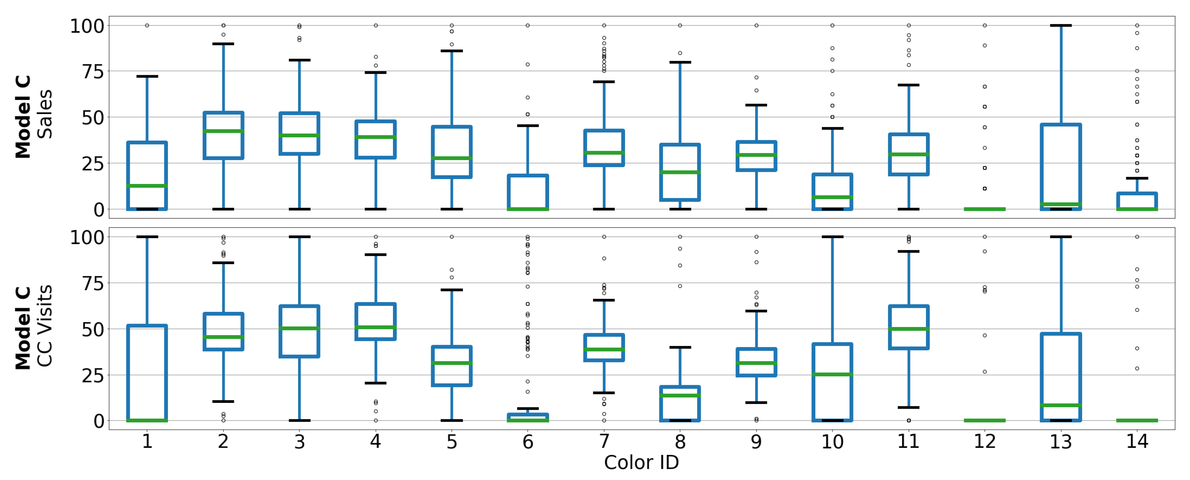
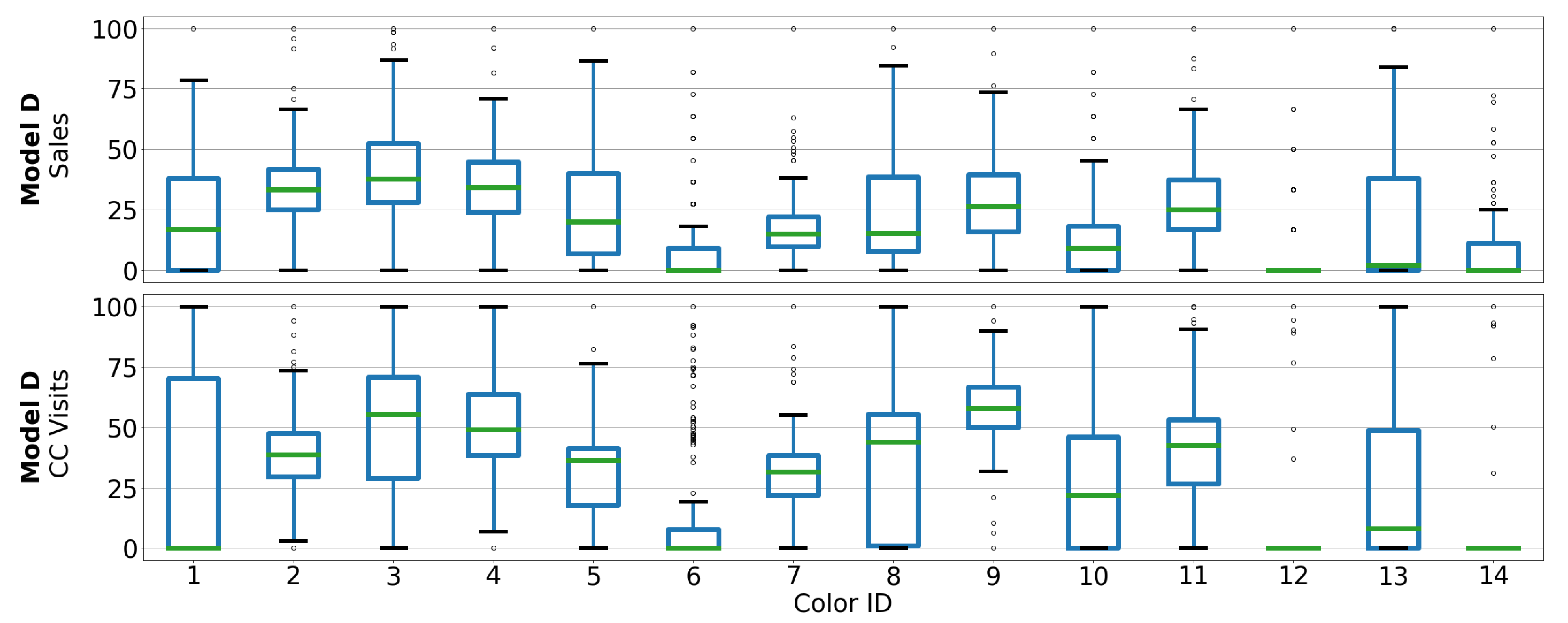
3.2. Dataset Description

Weekly data from 2 April 2017 until 2 February 2020 has been collected. It contains sales registrations and historic customer visits to the SEAT CC webpage within Spain. In total there are 149 observations. Data are shown in the best way to preserve the company’s confidentiality desire, but permitting interpretation. The weight of sold cars and CC visits per year and per car model is in

Table 2. Volume (%) of sales and CC visits for each car model of the dataset. Data are aggregated by car model when it is divided by year, and it is aggregated by year when it is divided by car model. Bold text represents the largest value of each column.

Year	Sales	CC Visits	Car Model	Sales	CC Visits
2017	19.61%	26.79%	Model A	26.08%	23.12%
2018	40.55%	44.44%	Model B	32.04%	30.68%
2019	36.53%	26.70%	Model C	28.16%	30.93%
2020	3.31%	2.06%	Model D	13.72%	15.26%

.

Figure 1, Figure 2, Figure 3 and Figure 4 show scaled boxplots of the colors of each car model. As it can be noticed, color distributions of sales and CC visits do not necessarily follow the same pattern. What it is easy to observe is those colors with anomalies, such as Color 8 from Figure 1, which barely has CC visits but was regularly sold; or Color 6 from Figure 2, with rare CC visits and sales.

For reasons better explained in Section 5, data have been divided into five different time chunks, with their corresponding test periods. The weekly behavior of sales and CC visits of each car variant per time chunk is shown in Figure 5, Figure 6, Figure 7 and Figure 8.

4. Methodology

This section describes the procedure that was created to measure the influence CC data have over sales. It can be followed by any automotive manufacturer with CC available. It is composed of three steps. Firstly, measuring the direct correlation between sales and CC data. Hence, performing sales predictions of each car variant within a test period. Finally, assessing results with respect to real forecast weekly color mixes sales. We are inspired by work [37] as a valid framework to compare different forecasting algorithms in the automotive industry.

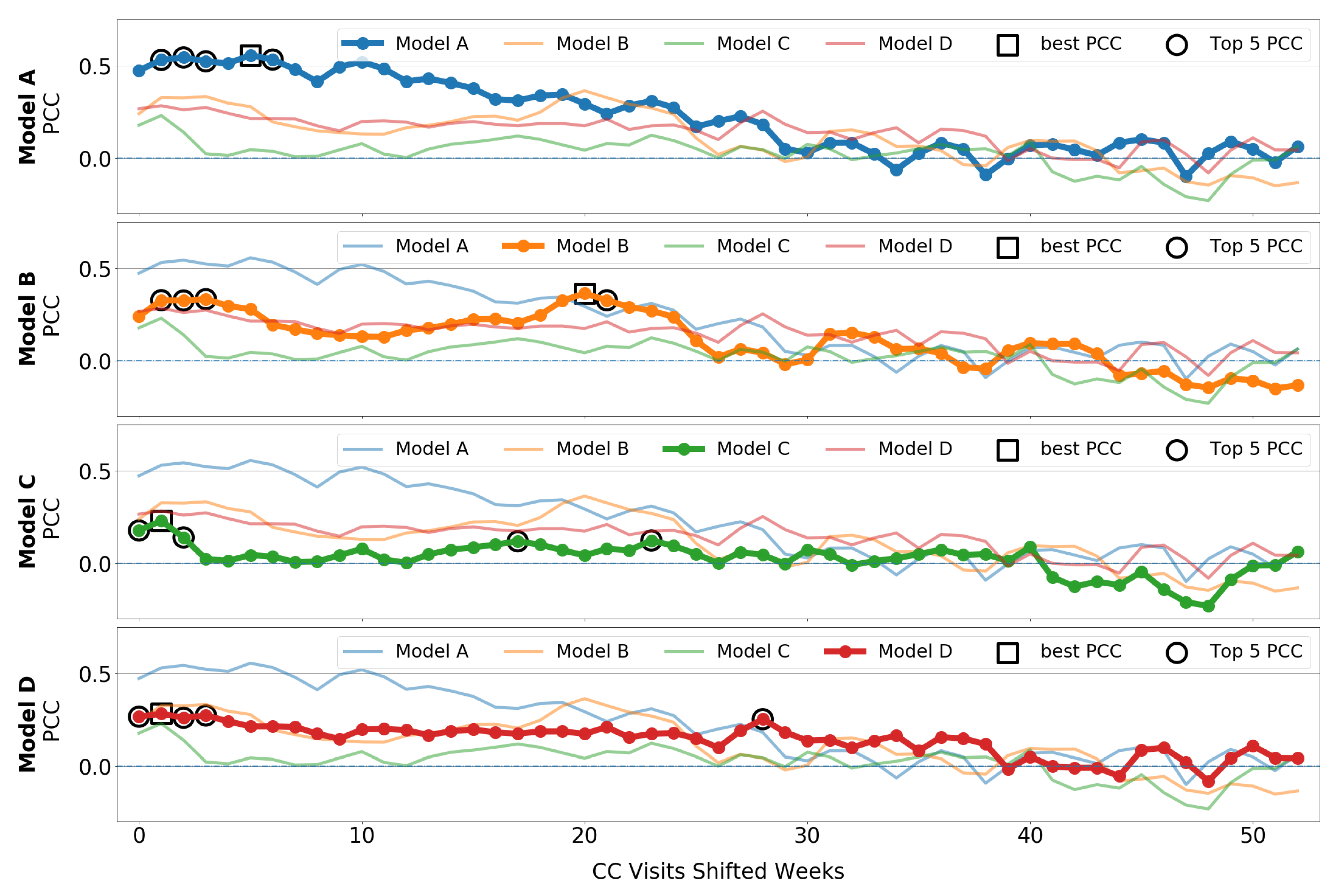
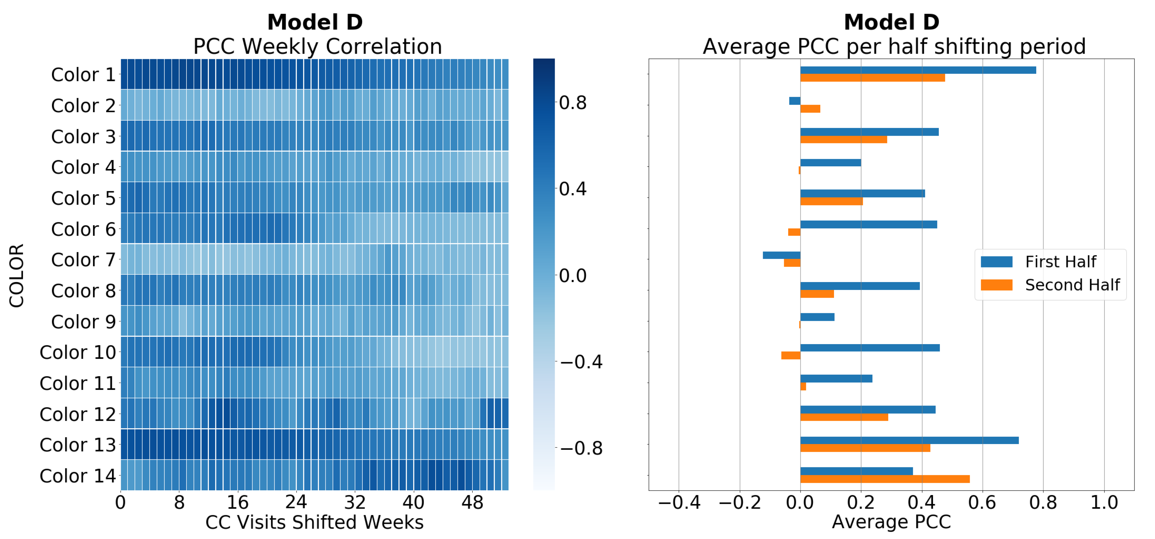
4.1. Correlation between Sales and CC Data

Firstly, both sales and CC data will be aggregated at the car-model level in the form of weekly time series. It is what we call the full-aggregation level. Hence, the PCCs of sales records and CC data are computed by shifting the online time series over a period of 52 weeks, i.e., a full year. The motivation is to find the period of maximum influence between sales and CC data. Nevertheless, we proceed with this strategy at the car-variant level. We expect to observe the same behavior in CC users, but reinforced. In other words, gaining more reliability about the influence of CC data over sales record.

Therefore, we will gain knowledge about the period of maximum correlation between both time series. It is studied at different granular levels, in order to provide more robustness. Hence, these learnings are employed to divide data into time chunks. Within each time chunk, the last month and a half defines the test period. Additionally, with this division, it is intended to face all the stages of the product life cycle: introduction, growth, maturity, and decline.

4.2. Forecasting Techniques

The next step to solve the research question is as follows. Within each time chunk, we have to define the test period. This month and a half of data will serve to predict the sales volume of each car variant. Hence, construction of forecast weekly color mix sales will be possible. They are defined as the percentage of sales each car variant has over the weekly sales volume.

These mixes are derived from a set of ML algorithms and statistical procedures. They are trained with the rest of the data of the corresponding time chunk. However, we distinguish between two techniques: univariate and multivariate. The first ones only consider past sales data. The latter ones include additionally the information from the automotive brand’s webpage. We use these techniques to perform the sales prediction of each car variant. We present the list of techniques used in this note.

• (Roll) ARIMA—Univariate: Statistical model constructed by (p) the dependent relationship between an observation and some number of lagged observations; (d) the use of differencing of raw observations; (q) the dependency between an observation and a residual error from a moving average model applied to lagged observations. Future estimations come from past data, not from independent variables. See [38] for a detailed explanation of the algorithm.
• (Roll) VARMAX—Multivariate: Extension of the VARMA model that also includes the modeling of exogenous variables. The latter ones are also called covariates and can be thought of as parallel input sequences that have observations at the same time steps as the original series, see [39] for a detailed explanation of the algorithm.
• XGBoost—Univariate/Multivariate: Efficient implementation of gradient boosting algorithm. Gradient boosting refers to a class of ensemble machine learning constructed from decision tree models. Trees are added one at a time to the ensemble and fit to correct the prediction errors made by prior models. Models are fit using any arbitrary differentiable loss function and gradient descent optimization algorithm, see [40] for a detailed explanation of the algorithm.

Inside each time chunk and the car variants belonging to it, some rules were fixed. Firstly, only those colors with any sales during the test period of each chunk were predicted. Hence, for those algorithms where it is possible to estimate in advanced the most precise parameters, such as ARIMA and Rolling ARIMA, autocorrelation function (acf) and partial autocorrelation function (pacf) were employed to obtain the moving average (q) and autoregressive parameter (p), respectively. Stationarity (d) of the time series is analyzed by means of the augmented Dickey–Fuller test, see references [41,42,43] for a detailed explanation. In case this procedure is unsuccessful, parameters (p,q) are estimated as first order, by default.

For multivariate algorithms VARMAX and Rolling VARMAX, acf and pacf were used as well, but for sales ($p_S$, $q_S$) and CC visits ($p_{CC}$, $q_{CC}$), individually. Thus, for the four pairs of parameter combinations, only the pair ($p_{xx}$, $q_{xx}$) with the lowest mean average error (MAE) was chosen. Prefix Rolling means that predictions are done one by one, augmenting the size of the training set. This approach is more robust than predicting all test sets at once.

Finally, for the case of algorithms of boosting nature, there were no shortcuts, and all parameter combinations ($la{g}_S$, $la{g}_{CC}$) within the range of the training set were evaluated. The purpose is to convert the forecasting time series problem into a supervised one. Hence, depending on parameter combination, and size of input changes. We select parameter combinations with the lowest mean average error (MAE). It has been decided to employ MAE as an evaluation metric because outliers might be found in the sales record of each variant and this metric is very resistant to these events.

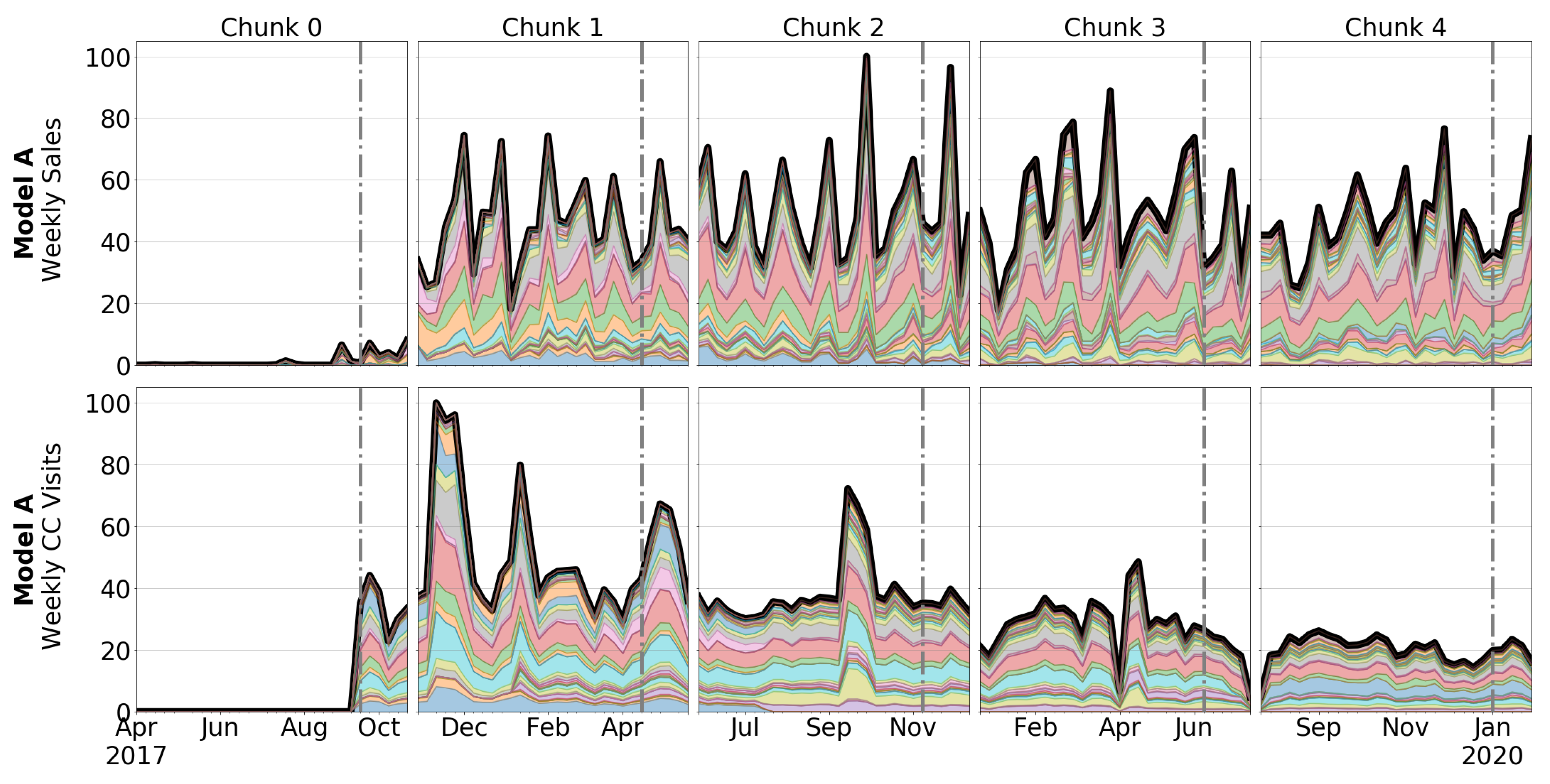
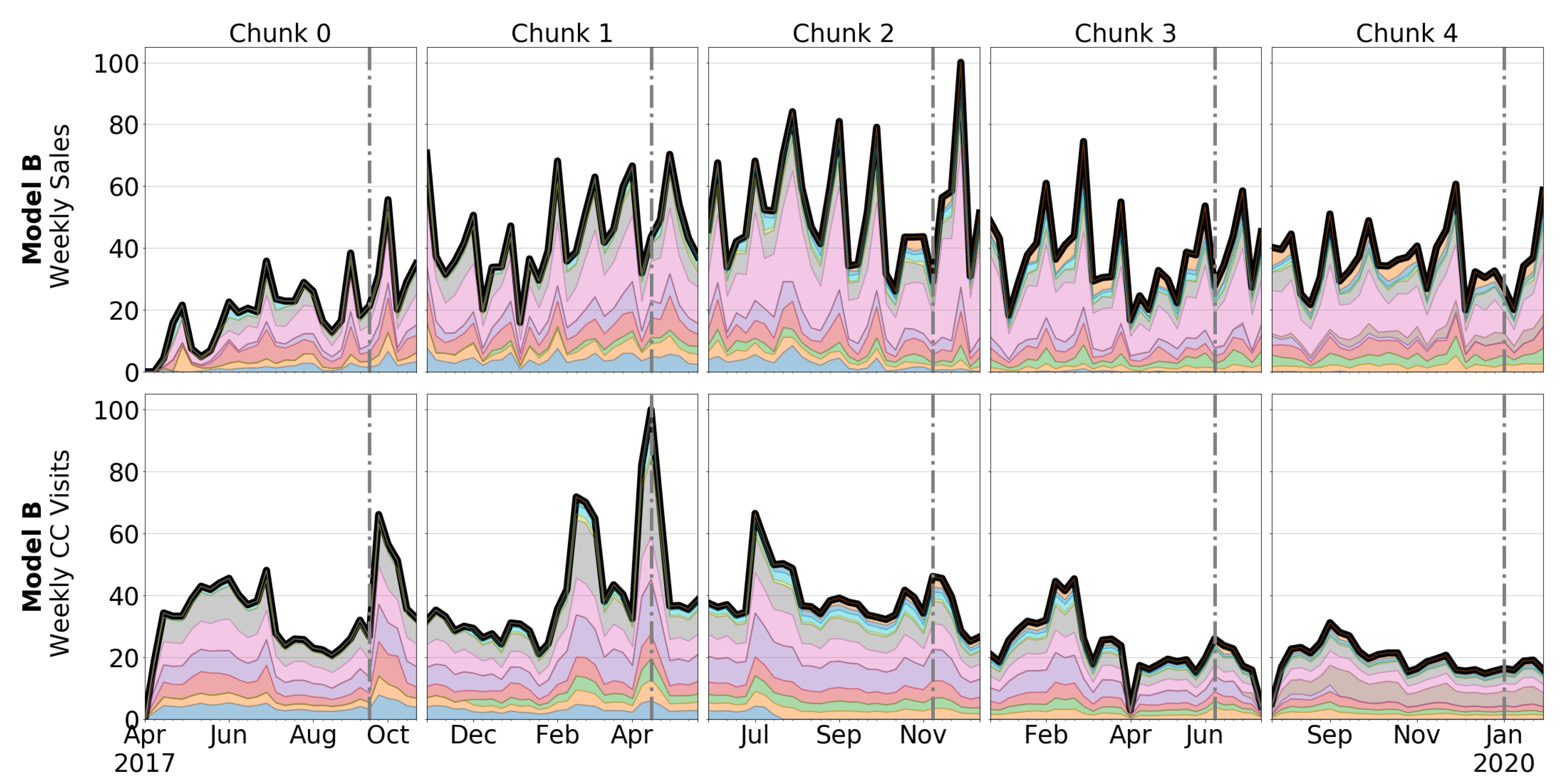
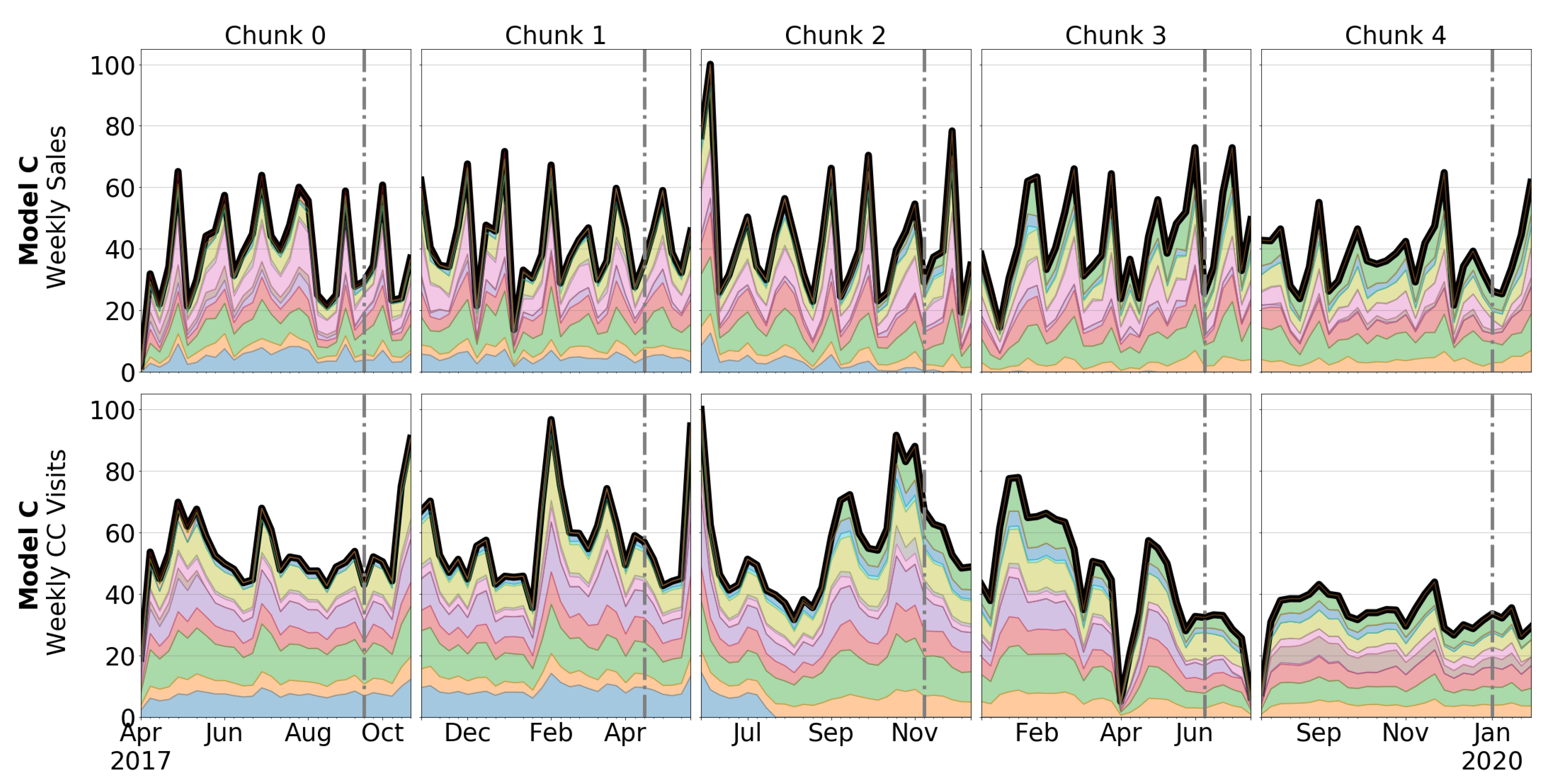
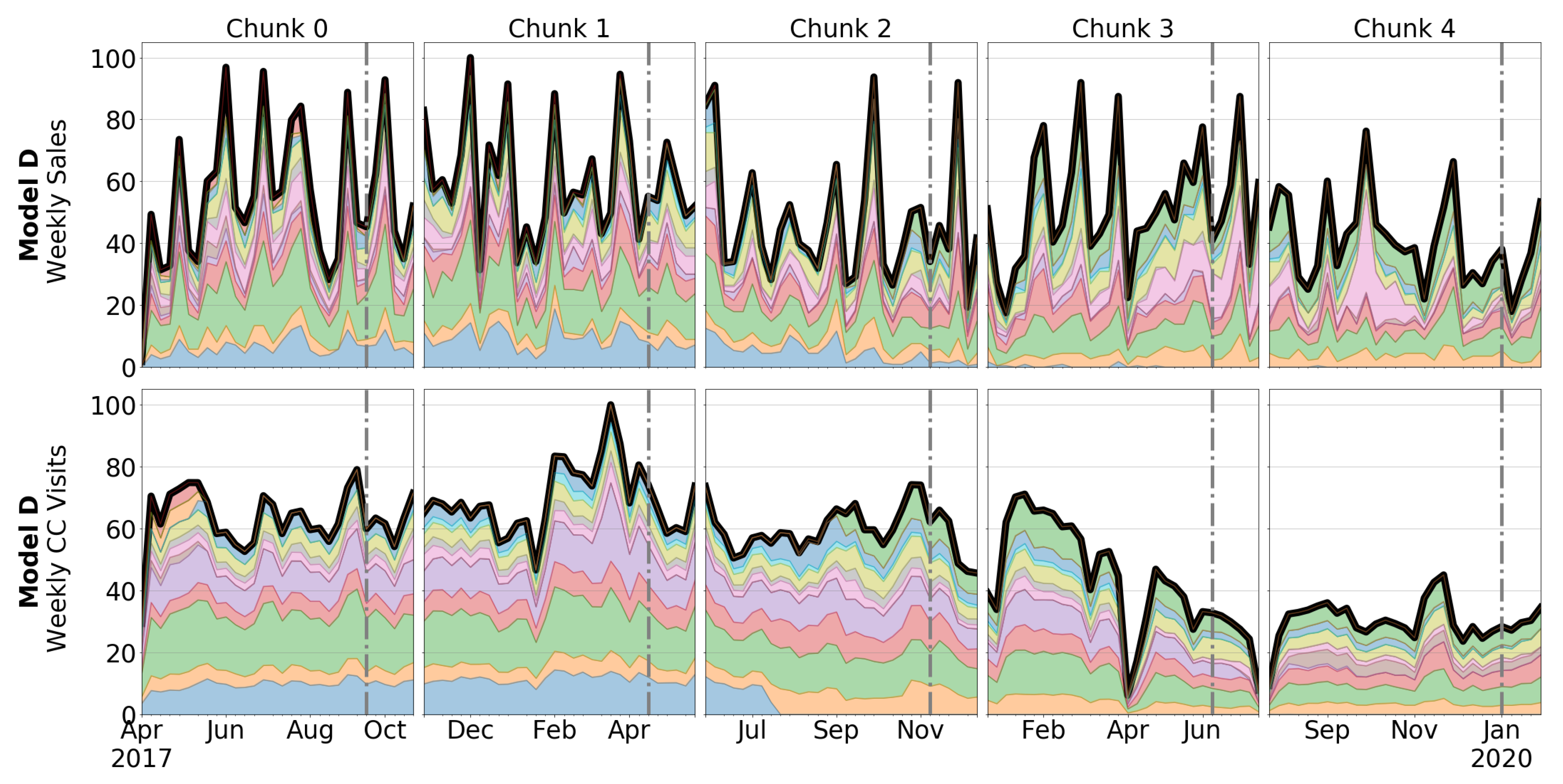
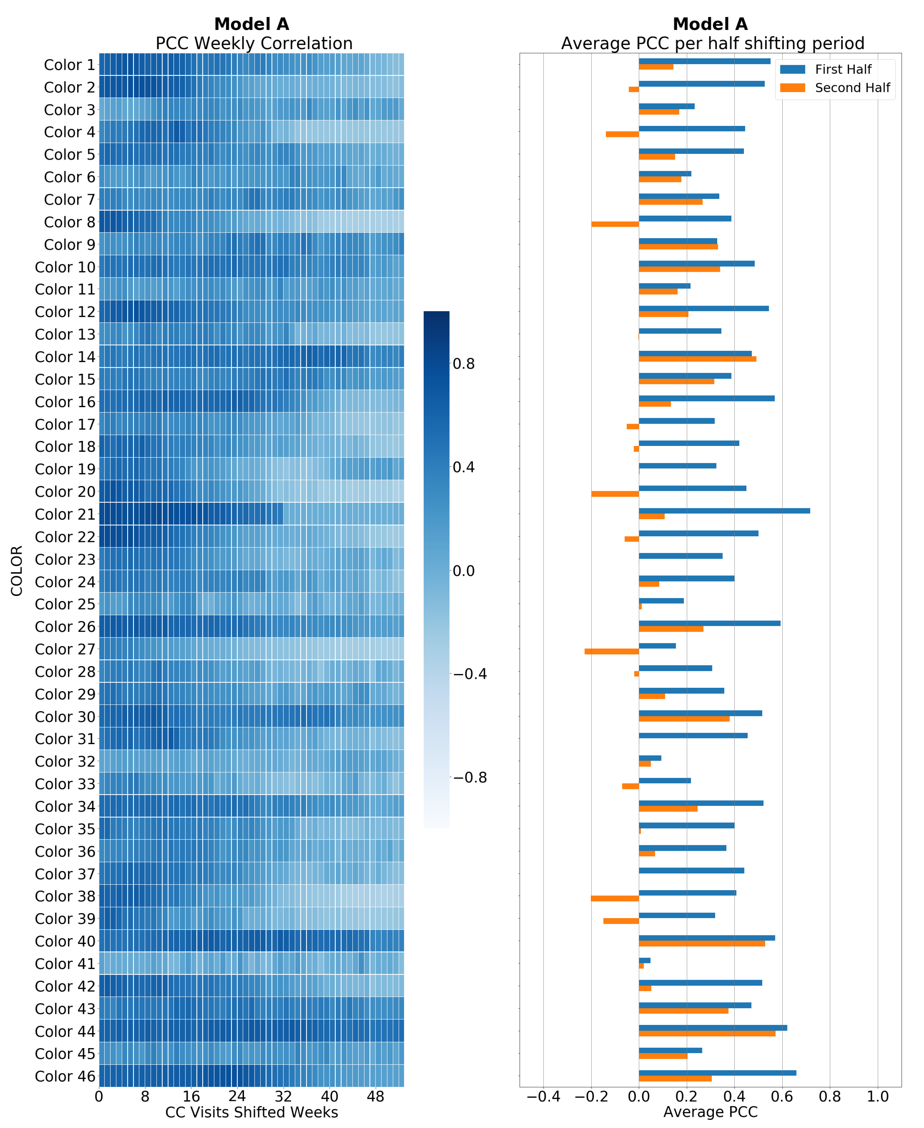
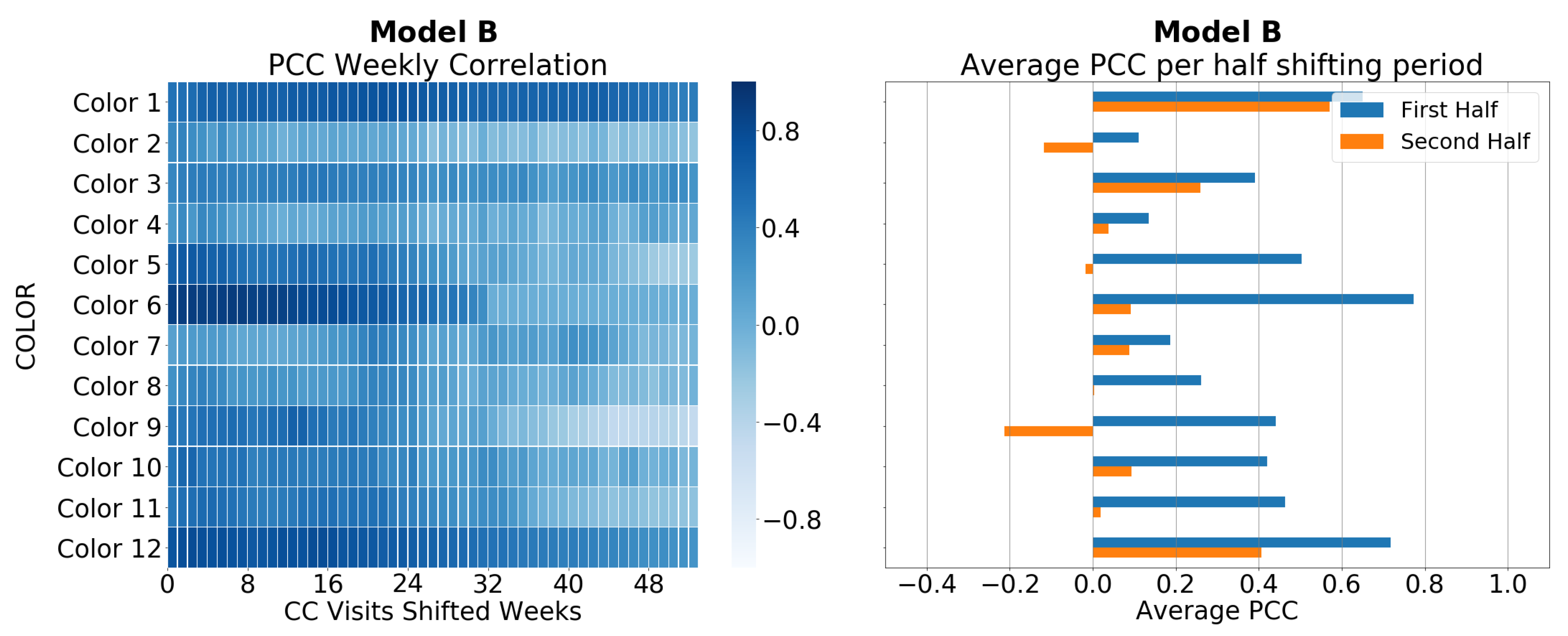
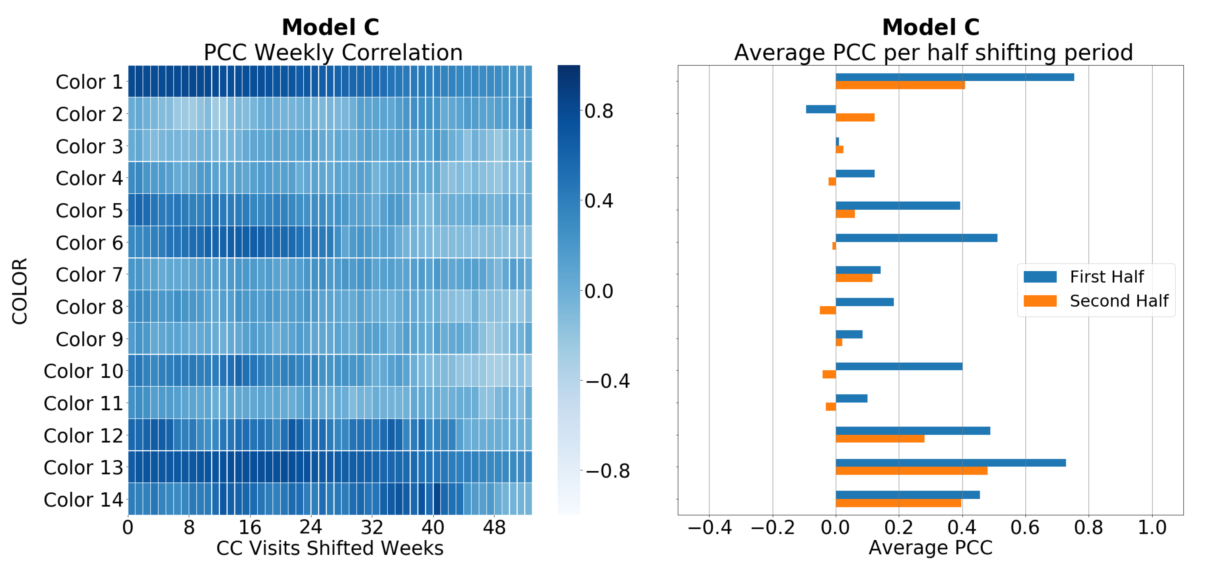
4.3. Weekly Color Mix Sales Procedure

Once the previous step is completed, these outcomes are assessed with respect to the real weekly color mix sales. Hence, the results got from univariate techniques will be compared to multivariate ones.

Traditional metrics such as MAE and root mean squared error (RMSE) were discharged because they are scale dependent. They are useless to compare different time chunks and car models. One solution arrives in the form of mean average percentage error (MAPE). However, this metric is not able to deal with zero values in any of the series. That is why we propose to compute the PCC between forecast and real mixes, as assessment metric.

Conclusions will arrive after following a sequential procedure. Firstly, the outputs are averaged over the total length of weeks and time chunks the dataset has. The second step consists of averaging, but over each time chunk. Acting in this way, we gain more detail about the performance of each technique. Lastly, the assessment process finishes with the third step. In this level, we count what technique provides the best metric for each week of the test set within each chunk.

5. Results

This section shows the outcomes derived from validating CC data as a reliable information source for automotive OEMs. Firstly, the correlation analysis at different granular levels is exposed. Then, the forecasting performance of the different techniques is shown. Finally, numbers related to the assessment procedure of weekly color mix sales are presented.

5.1. Correlation between Sales and CC Data

Regarding the full-aggregation level, the results in Figure 9 show that positive PCC exists for all car models under analysis. Although it does not have the strength we would expect. None of our four car models reaches a PCC peak close to the unit, being Model A the one with the largest PCC. However, it is possible to extract one conclusion. For all car models, the largest PCC is within the first half of the shifting period, as well as the rest of the top five largest PCCs. The unique exception is for Model D, where one of these top five PCCs occur at the 28th shifted week. Hence, we conclude that purchase likelihood increases within a period of up to 6 months after visiting the CC webpage.

For car variant’s time series, results are displayed from Figure 10, Figure 11, Figure 12 and Figure 13, each one representing one car model. At this granular level, the behavior of PCC is similar to the previous one. Correlation is stronger in the first half of the shifting period than in the second half, as it occurs at the full-aggregation level. However, as well, larger values are reached than at the previous granular level, meaning a stronger correlation. Combining this information, it is possible to validate the previous conclusion with more confidence at the car-variant level. Therefore, we will divide the time series into five time chunks of six-month size, where the last month and a half defines the test period.

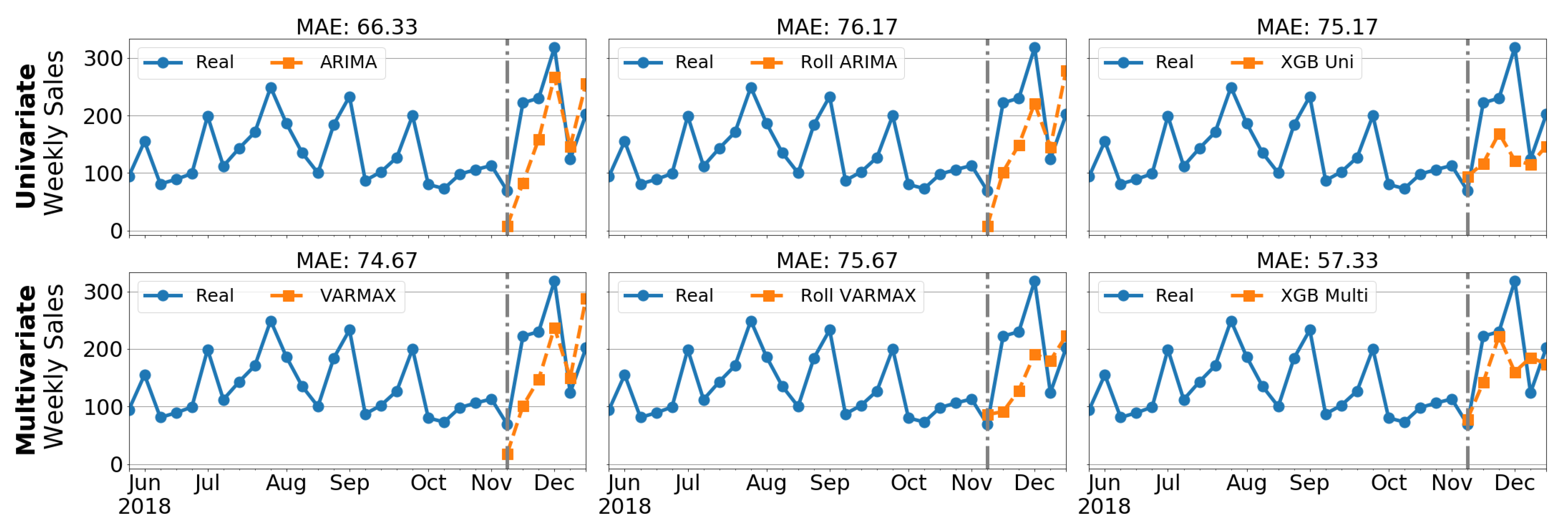
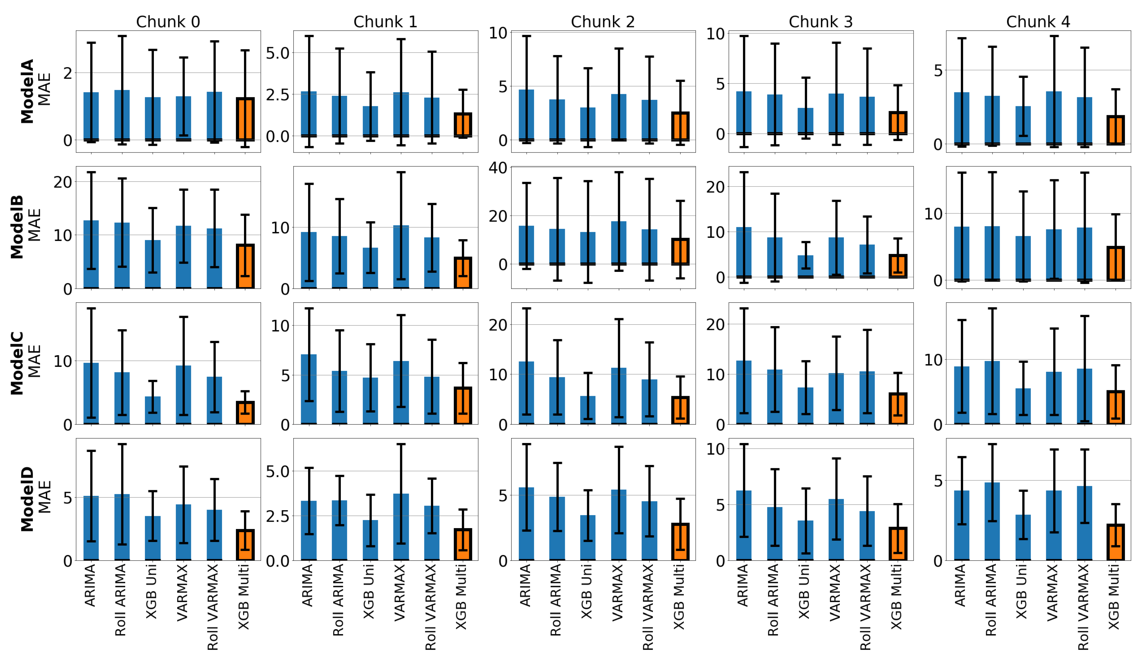
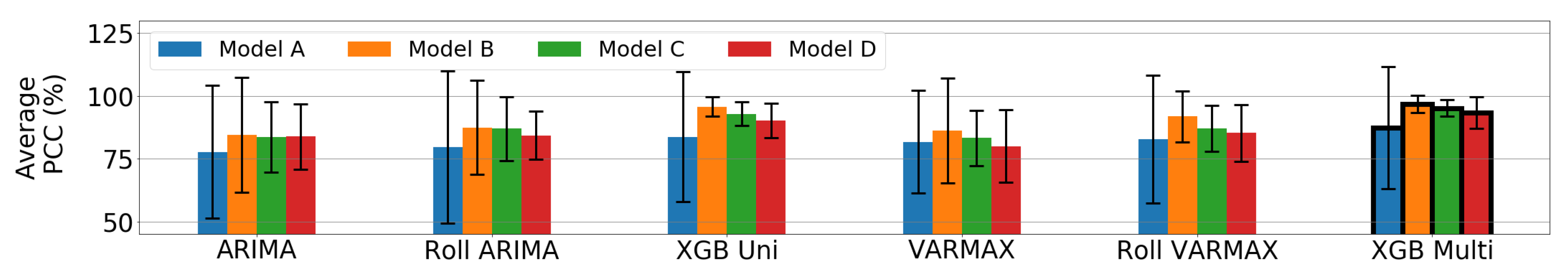
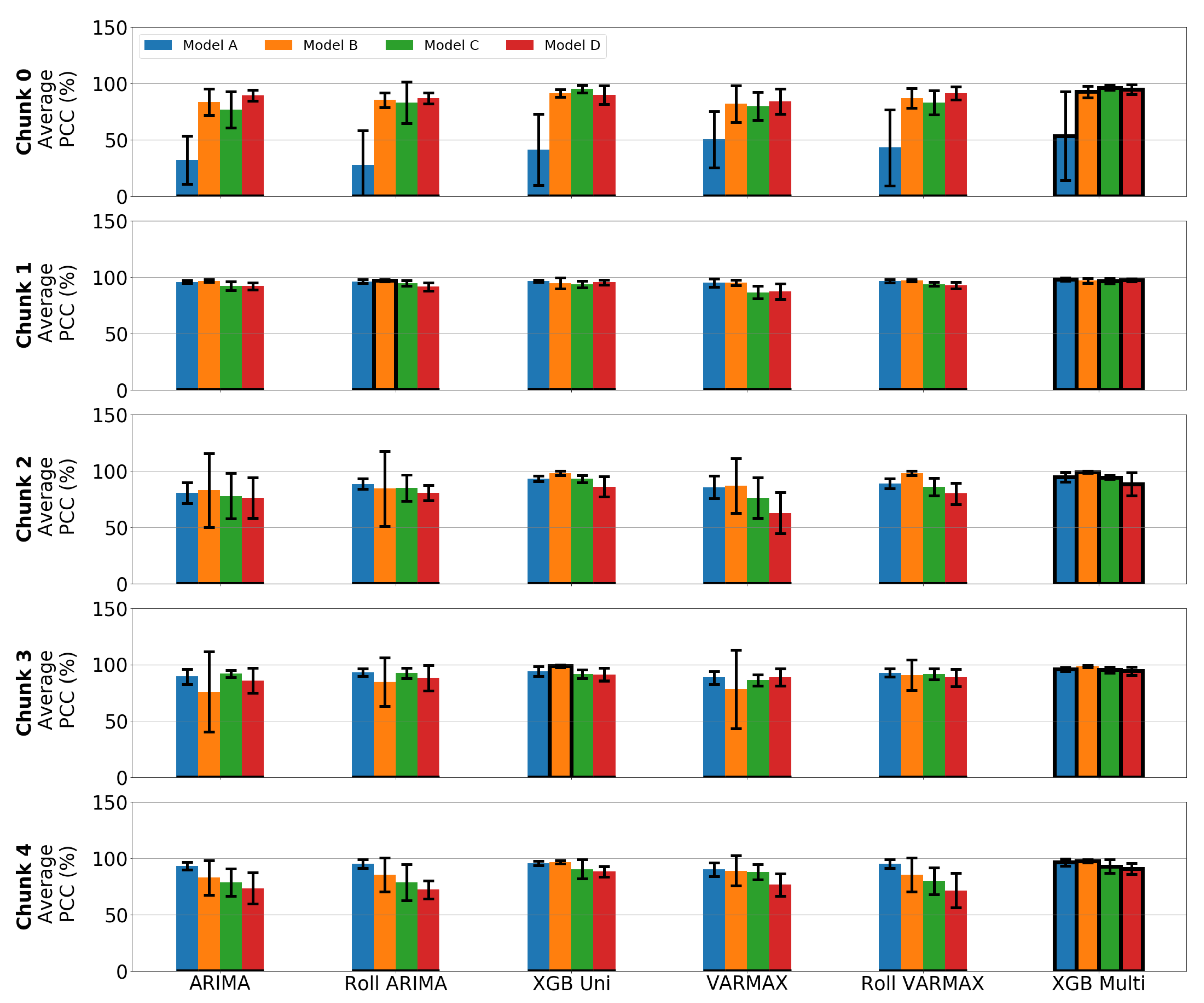
5.2. Forecasting Performance

At a first step, we present in Figure 14 the outcomes derived from the diverse forecasting techniques. For simplicity, we only illustrate this stage with the best seller car variant. We refer to Model B and Color 7 at time chunk 2. The car variant’s sales were 1165 units during the test period associated with this time chunk. It lays from the week of 11 November to the week of 16 December 2018. The best technique is one of the multivariate ones. XGBoost Multi has the lowest MAE. When errors are averaged per class, the second category has the lowest error. It opened a path to prove that CC data can be considered reliable information.

We extend this error analysis to the totality of the dataset. Figure 15 presents the aggregated MAE per car model and time chunk. Accuracy metric averages the one obtained by each car variant. At this level, the previous pattern is repeated. Multivariate techniques provides the best outputs. The largest variability is observed in Model A, but it has the lowest MAE in order of magnitude.

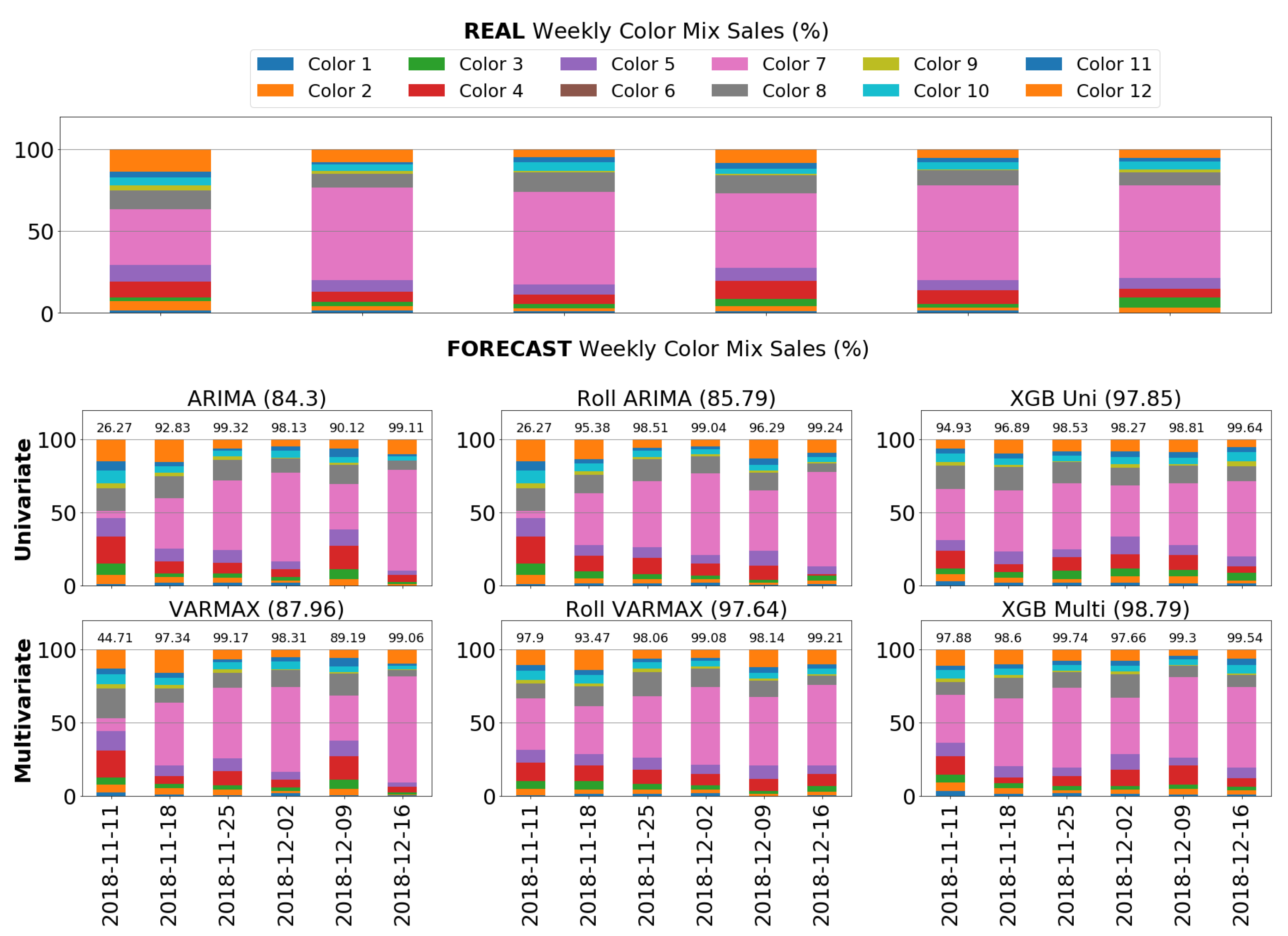
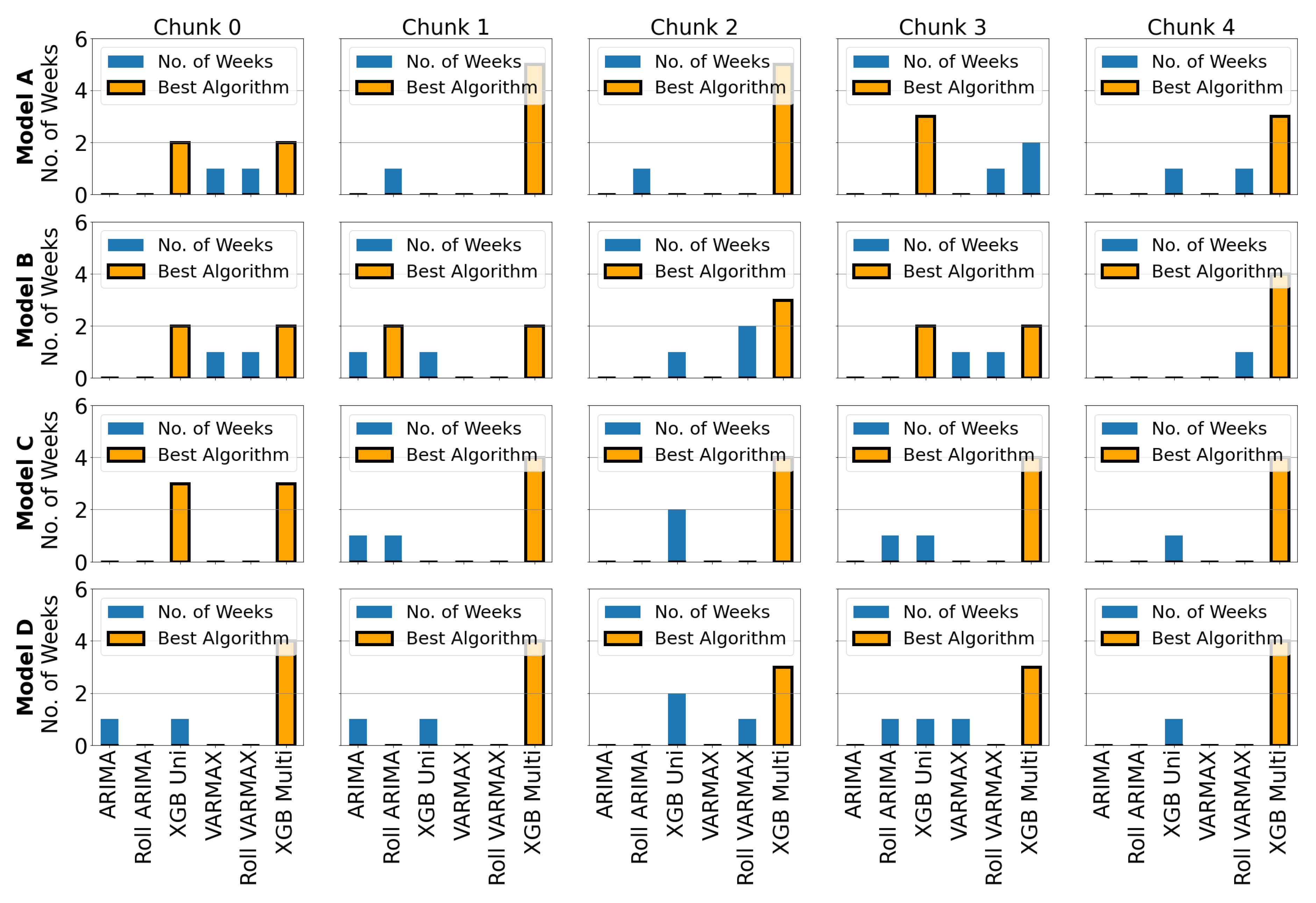
5.3. Weekly Color Mix Sales Assessment

Once forecasting has been tested, we continue with the weekly color mix sales assessment. We need this stage to corroborate the previous outputs. Data from the automotive brand’s webpage is proving its validity as a reliable source. We follow the same structure as before. It is presented a specific car model. Hence, the performance evaluation is extended to the rest of data.

A car model from the best seller car variant in the same time chunk was chosen to display in Figure 16. Forecast sales volume of each car variant, done by each forecasting technique, were employed to build weekly color mix sales. Hence, within each week of the test period, similarity with respect to the real one was measured. We decided to use PCC as a comparison metric between these two mixes. In this example, the previous pattern is repeated. Larger correlations between real weekly color mix sales and forecast ones are achieved thanks to incorporating CC data.

Afterward, we computed the averaged performance over the total length of weeks and time chunks of the different forecasting techniques. This stage is shown in Figure 17 for all car models. At this point, the metric provided by one of the multivariate method outperforms the rest of the results. Nevertheless, XGBoost Univariate would be a good candidate on the side of univariate techniques. Model A has the largest dispersion caused by the first time chunk. This age is the launch period for this car model.

In the second phase, the assessment occurs at the time-chunk level. The outcomes of each forecasting technique are averaged over this time level. The intention is to gain more details about the performance. This behavior is displayed in Figure 18. For all car models in the grid, the XGBoost Multivariate technique provides larger outputs in the majority of time chunks. Exceptions occur for Model B at time chunks 1 and 3. The best metric is achieved by univariate techniques such as Rolling ARIMA and XGBoost Univariate, respectively. That is why it is necessary to proceed with the assessment procedure.

The evaluation of weekly color mix sales finishes with the third step. The summary of this count is shown in Figure 19. Three different scenarios are distinguished. The first scenario is the most common: one of multivariate forecasting technique provides the best results for the vast majority of weeks within each time chunk. The second scenario corresponds to a draw between two techniques, but multivariate is always one of the participants in the tie. Finally, the third scenario is the most bizarre due to it only performing the best in one case. For Model A and time chunk 3, the best count was provoked by one of the univariate techniques. Nevertheless, we have learned in the second step of the forecasting assessment that the multivariate technique gives the best average metric in these circumstances.

6. Discussion

The analysis of the correlation between sales and CC visits at different granular levels was fundamental. Results at the full-aggregation level show that users spend from 1 to 6 months visiting the webpage and this period has a positive impact on sales. Our results are aligned with the discoveries of other authors. Paper [24] was able to find a correlation in the entertainment industry in terms of weeks. For the financial sector, the correlation with online data is found at the day level, as supported in [25]. These timeframes are considered normal for these products. However, in the car purchase process, the period expands considerably, as it is common in high-implication products. The car model most benefiting from this correlation is Model A. Furthermore, the correlation is even larger when the granularity augments to the car-variant level. The influence of CC visits over sales during this interval is reinforced. These learnings were very helpful to proceed with the forecasting at different time chunks.

From the two different classes of forecasting techniques, univariate and multivariate, the latter proves to be more robust. In terms of car variants sales prediction, XGBoost Multivariate has the best performance. It has been proved at the bestseller car variant and averaged for each time chunk and car model. In Figure 15, it is noticed an MAE reduction from best to worst techniques that range from tiny 0.25, in the case of Model A at time chunk 0, up to 7.5 points, in case of Model B at time chunk 2. We associate the smallest reduction to the fact that time chunk 0 for Model A represents the launch age of the vehicle. In other words, not all car variants were available to sell, but they were for consulting online. These outputs where predictions supported by online data outperform are consistent with the literature described in Section 2. However, none of these studies used CC data as the input. It is a second step to prove this source as reliable information, where forecasting was the best way to confirm it.

Finally, the last stage consisted of the weekly color mix sales comparison. We propose this approach to measure the trustworthiness of CC data. No evidence of this methodology was found in the literature. In all the assessment procedure, the multivariate technique was highlighted as the best one. In Figure 17, it provides improvement from nearly 9.6, in Model A, to 13.2 points, in Model D, for the PCC metric. Additionally, when evaluation occurs at the time-chunk level, in the case shown in Figure 18, the largest metric improvement reflects a variation of 25 points. It is noticed in Model D at time chunk 2. All the aforementioned reasoning leads us to validate that CC data are a reliable source to capture in advance customers’ demand from automotive OEMs.

Moreover, the preprocess of boosting-based algorithms is simpler than the rest of the algorithms. On the other hand, autoregressive and moving average-based algorithms deal with more difficulties, rather than univariate or multivariate. This is another reason to suggest XGBoost Multivariate as the best forecasting algorithm. The chosen metric to perform the assessment of the results was valid. Weekly color mixes sales could be compared for different algorithms, car models, and time chunks due to scale independence. Additionally, the metric manifests a similar pattern when it was tested for the total length of the dataset and per chunk level.

7. Conclusions

In conclusion, the results show that the addition of CC data is beneficial to automotive OEMs. The new methodology presented in this paper demonstrates the influence of this input. Although numbers of this note is exclusive to one company, the rest of the automotive OEMs can take advantage of the procedure.

Firstly, correlation analysis between this source and sales shows a period of maximum influence. Results are consistent at different granular levels. Users consult the online tool from 1 to 6 months before the purchase date. Secondly, forecasting is the other tool employed to validate CC data. Thanks to prediction, it is proved that the best outcomes are given by techniques that include CC data. It has been tested at a single car variant level, but as well per car model and time chunk. In both cases, best multivariate technique has no rivals. Afterward, forecast weekly color mix sales are calculated. Hence, they were under an assessment process against the real ones. This multistage procedure validates the multivariate technique as the best one.

Although employing data from the CC webpage of the automotive OEM may cause concerns, we have overpassed them. Filtering raw data to select the registers that completed the full journey was helpful for: (a) computing PCC between CC visits and sales records; (b) performing sales predictions of the different car variants; (c) building and comparing weekly color mix sales.

However, there is still room for improving these outcomes. Future research in this area should include (a) the addition of the commercial objectives of the company, they may explain anomaly behaviors of the sales; (b) CC data divided by test-drives requested, as a sign of real interest into finishing purchase; (c) information derived directly from dealers, as relevant actors involved in the acquisition process, such as how many test drives were really done or commercial offers proposed to customers. We suggest employing data belonging to the company, as a way of avoiding third-party sources, and growing the literature’s knowledge.

Finally, we propose, as future path, to put this study into production and take advantage of the results to adapt the factory production according to them. The goal is to achieve maximum matching between the composition of estimated company inventory and the forecast mix sales. In short term prediction, production modification is only possible in non-restricted items, such as the color of the vehicle.

References

1. Zhang, Y.; Hara, T. Predicting E-commerce Item Sales With Web Environment Temporal Background. In Proceedings of the 24th International Conference on Business Information Systems, BIS 2021, Hannover, Germany, 15–17 June 2021; Abramowicz, W., Auer, S., Lewanska, E., Eds.; 2021; pp. 233–243. [Google Scholar] [CrossRef]
2. Huang, Y.T.; Pai, P.F. Using the Least Squares Support Vector Regression to Forecast Movie Sales with Data from Twitter and Movie Databases. Symmetry 2020, 12, 625. [Google Scholar] [CrossRef] [Green Version]
3. Ling, L.; Zhang, D.; Chen, S.; Mugera, A. Can online search data improve the forecast accuracy of pork price in China? J. Forecast. 2020, 39, 671–686. [Google Scholar] [CrossRef]
4. Havranek, T.; Zeynalov, A. Forecasting tourist arrivals: Google Trends meets mixed-frequency data. Tour. Econ. 2019, 27, 129–148. [Google Scholar] [CrossRef] [Green Version]
5. Sujo, J.; Ribé, E.; Cardona, X. CAIT: A Predictive Tool for Supporting the Book Market Operation Using Social Networks. Appl. Sci. 2021, 12, 366. [Google Scholar] [CrossRef]
6. Beracha, E.; Wintoki, M.B. Forecasting residential real estate price changes from online search activity. J. Real Estate Res. 2013, 35, 283–312. [Google Scholar] [CrossRef]
7. Sun, D.; Du, Y.; Xu, W.; Zuo, M.; Zhang, C.; Zhou, J. Combining Online News Articles and Web Search to Predict the Fluctuation of Real Estate Market in Big Data Context. Pac. Asia J. Assoc. Inf. Syst. 2013, 6, 19–37. [Google Scholar] [CrossRef]
8. Dietzel, M.; Braun, N.; Schäfers, W. Sentiment-based commercial real estate forecasting with Google search volume data. J. Prop. Invest. Financ. 2014, 32, 540–569. [Google Scholar] [CrossRef] [Green Version]
9. Wei, Y.; Cao, Y. Forecasting house prices using dynamic model averaging approach: Evidence from China. Econ. Model. 2017, 61, 147–155. [Google Scholar] [CrossRef]
10. Venkataraman, M.; Panchapagesan, V.; Jalan, E. Does internet search intensity predict house prices in emerging markets? A case of India. Prop. Manag. 2018, 36, 103–118. [Google Scholar] [CrossRef]
11. Rizun, N.; Baj-Rogowska, A. Can Web Search Queries Predict Prices Change on the Real Estate Market? IEEE Access 2021, 9, 70095–70117. [Google Scholar] [CrossRef]
12. Fogliatto, F.S.; da Silveira, G.J.C.; Borenstein, D. The mass customization decade: An updated review of the literature. Int. J. Prod. Econ. 2012, 138, 14–25. [Google Scholar] [CrossRef]
13. Pil, F.; Holweg, M. The Second Century Reconnecting Customer and Value Chain through Build-to-Order Moving beyond Mass and Lean Production in the Auto Industry; The MIT Press: Cambridge, MA, USA, 2005. [Google Scholar] [CrossRef]
14. Zhang, L.; Lee, C.; Akhtar, P. Towards customization: Evaluation of integrated sales, product, and production configuration. Int. J. Prod. Econ. 2020, 229, 107775. [Google Scholar] [CrossRef]
15. Sa-Ngasoongsong, A.; Bukkapatnam, S.; Kim, J.; Iyer, P.; Suresh, R.P. Multi-step sales forecasting in automotive industry based on structural relationship identification. Int. J. Prod. Econ. 2012, 140, 875–887. [Google Scholar] [CrossRef]
16. Wochner, S.; Grunow, M.; Staeblein, T.; Stolletz, R. Planning for Ramp-ups and New Product Introductions in the Automotive Industry: Extending Sales and Operations Planning. Int. J. Prod. Econ. 2016, 182, 372–383. [Google Scholar] [CrossRef]
17. Irwin, J. Survey Shows Color Key Factor for 88% of Vehicle Shoppers. Available online: https://www.wardsauto.com/dealers/survey-shows-color-key-factor-88-vehicle-shoppers (accessed on 23 June 2021).
18. Bravais, A. Analyse Mathématique sur les Probabilités des Erreurs de Situation d’un Point; Impr. Royale: Paris, France, 1844. [Google Scholar]
19. Spearman, C. The proof and measurement of association between two things. By C. Spearman, 1904. Am. J. Psychol. 1987, 100, 441–471. [Google Scholar] [CrossRef]
20. Shannon, C.E. A mathematical theory of communication. Bell Syst. Tech. J. 1948, 27, 379–423. [Google Scholar] [CrossRef] [Green Version]
21. Sun, S.; Zhang, C.; Zhang, Y. Traffic Flow Forecasting Using a Spatio-temporal Bayesian Network Predictor. In Lecture Notes in Computer Science; Springer: Berlin/Heidelberg, Germany, 2005; pp. 273–278. [Google Scholar] [CrossRef]
22. Liu, Y.; Wang, W.; Ghadimi, N. Electricity Load Forecasting by an Improved Forecast Engine for Building Level Consumers. Energy 2017, 139, 18–30. [Google Scholar] [CrossRef]
23. Sheugh, L.; Alizadeh, S. A note on pearson correlation coefficient as a metric of similarity in recommender system. In Proceedings of the 2015 AI & Robotics (IRANOPEN), Qazvin, Iran, 12 April 2015; pp. 1–6. [Google Scholar] [CrossRef]
24. Goel, S.; Hofman, J.M.; Lahaie, S.; Pennock, D.M.; Watts, D.J. Predicting consumer behavior with Web search. Proc. Natl. Acad. Sci. USA 2010, 107, 17486–17490. [Google Scholar] [CrossRef] [Green Version]
25. Bordino, I.; Battiston, S.; Caldarelli, G.; Cristelli, M.; Ukkonen, A.; Weber, I. Web Search Queries Can Predict Stock Market Volumes. PLoS ONE 2012, 7, e040014. [Google Scholar] [CrossRef] [Green Version]
26. Wei, D.; Geng, P.; Ying, L.; Shuaipeng, L. A prediction study on e-commerce sales based on structure time series model and web search data. In Proceedings of the 26th Chinese Control and Decision Conference (2014 CCDC), Changsha, China, 31 May–2 June 2014; pp. 5346–5351. [Google Scholar] [CrossRef]
27. Punjabi, S.; Shetty, V.; Pranav, S.; Yadav, A. Sales Prediction using Online Sentiment with Regression Model. In Proceedings of the 2020 4th International Conference on Intelligent Computing and Control Systems (ICICCS), Madurai, India, 13–15 May 2020; pp. 209–212. [Google Scholar] [CrossRef]
28. Pai, P.F.; Liu, C.H. Predicting Vehicle Sales by Sentiment Analysis of Twitter Data and Stock Market Values. IEEE Access 2018, 6, 57655–57662. [Google Scholar] [CrossRef]
29. Varian, H.; Choi, H. Predicting the Present with Google Trends. Econ. Rec. 2009, 88, 2–9. [Google Scholar] [CrossRef] [Green Version]
30. Kim, D.; Woo, J.; Shin, J.; Lee, J.; Kim, Y. Can search engine data improve accuracy of demand forecasting for new products? Evidence from automotive market. Ind. Manag. Data Syst. 2019, 119, 1089–1103. [Google Scholar] [CrossRef]
31. Wachter, P.; Widmer, T.; Klein, A. Predicting Automotive Sales using Pre-Purchase Online Search Data. ACSIS 2019, 18, 569–577. [Google Scholar] [CrossRef] [Green Version]
32. Fantazzini, D.; Toktamysova, Z. Forecasting German car sales using Google data and multivariate models. Int. J. Prod. Econ. 2015, 170, 97–135. [Google Scholar] [CrossRef] [Green Version]
33. Graevenitz, G.; Helmers, C.; Millot, V.; Turnbull, O. Does Online Search Predict Sales? Evidence from Big Data for Car Markets in Germany and the UK. SSRN Electron. J. 2016. [Google Scholar] [CrossRef]
34. Wijnhoven, F.; Plant, O. Sentiment Analysis and Google Trends Data for Predicting Car Sales. In Proceedings of the 38th International Conference on Information Systems, Seoul, Korea, 10 December 2017; pp. 1–16. [Google Scholar]
35. Zhang, C.; Tian, Y.X.; Fan, L.W. Improving the Bass model’s predictive power through online reviews, search traffic and macroeconomic data. Ann. Oper. Res. 2020, 295, 881–922. [Google Scholar] [CrossRef]
36. SEAT, S.A. (2020, February 12) Informe Anual 2019. Available online: https://www.seat.es/content/dam/countries/es/seat-website/sobre-seat/reporte-anual/pdf/others-annual_report_2019_full-NA-NA-NA-march-2020.pdf (accessed on 29 June 2022).
37. Gonçalves, J.; Cortez, P.; Carvalho, M.; Frazão, N. A multivariate approach for multi-step demand forecasting in assembly industries: Empirical evidence from an automotive supply chain. Decis. Support Syst. 2020, 142, 113452. [Google Scholar] [CrossRef]
38. Perktold, J.; Seabold, S.; Taylor, J. statsmodels.tsa.arima.model.ARIMA. Available online: https://www.statsmodels.org/devel/generated/statsmodels.tsa.arima.model.ARIMA.html (accessed on 29 June 2022).
39. Perktold, J.; Seabold, S.; Taylor, J. statsmodels.tsa.statespace.varmax.VARMAX. Available online: https://www.statsmodels.org/devel/generated/statsmodels.tsa.statespace.varmax.VARMAX.html?highlight=varmax (accessed on 29 June 2022).
40. XGBoost Developers. (Revision 5d92a7d9) XGBoost Documentation. Available online: https://xgboost.readthedocs.io/en/stable/index.html (accessed on 29 June 2022).
41. Perktold, J.; Seabold, S.; Taylor, J. statsmodels.tsa.stattools.acf. Available online: https://www.statsmodels.org/devel/generated/statsmodels.tsa.stattools.acf.html?highlight=acf (accessed on 29 June 2022).
42. Perktold, J.; Seabold, S.; Taylor, J. statsmodels.tsa.stattools.pacf. Available online: https://www.statsmodels.org/devel/generated/statsmodels.tsa.stattools.pacf.html?highlight=pacf (accessed on 29 June 2022).
43. Perktold, J.; Seabold, S.; Taylor, J. statsmodels.tsa.stattools.adfuller. Available online: https://www.statsmodels.org/devel/generated/statsmodels.tsa.stattools.adfuller.html?highlight=adfuller (accessed on 29 June 2022).
Figure 1. Scaled boxplot of sales (upper) and CC visits (lower) from each color of Model A.
Forecasting 04 00034 g001
Figure 2. Scaled boxplot of sales (upper) and CC visits (lower) from each color of Model B.
Forecasting 04 00034 g002
Figure 3. Scaled boxplot of sales (upper) and CC visits (lower) from each color of Model C.
Forecasting 04 00034 g003
Figure 4. Scaled boxplot of sales (upper) and CC visits (lower) from each color of Model D.
Forecasting 04 00034 g004
Figure 5. Weekly sales (upper) and CC visits (lower) from Model A. Each layer represents a color. The grey dash-dotted line reflects the beginning of test period.
Forecasting 04 00034 g005
Figure 6. Weekly sales (upper) and CC visits (lower) from Model B. Each layer represents a color. The grey dash-dotted line reflects the beginning of test period.
Forecasting 04 00034 g006
Figure 7. Weekly sales (upper) and CC visits (lower) from Model C. Each layer represents a color. The grey dash-dotted line reflects the beginning of test period.
Forecasting 04 00034 g007
Figure 8. Weekly sales (upper) and CC visits (lower) from Model D. Each layer represents a color. The grey dash-dotted line reflects the beginning of test period.
Forecasting 04 00034 g008
Figure 9. Pearson correlation coefficient (PCC) after shifting CC visits time series over sales time series at full aggregated time series level. Each row represents a car model in this order: Model A, Model B, Model C, and Model D. The solid-dotted line refers to PCC for each shifted week. A square mark signals the largest positive PCC. Circle marks point the rest of top 5 largest positive PCC.
Forecasting 04 00034 g009
Figure 10. Pearson correlation coefficient (PCC) for Model A and its colors. The left plot shows heatmap of the PCC value for each shifting week of the webpage visits time series over sales time series of each car variant. A darker color means largest PCC values. The right plot shows pair of horizontal bars per each color. These horizontal bars represent the average PCC in each half of the shifting period.
Forecasting 04 00034 g010
Figure 11. Pearson correlation coefficient (PCC) for Model B and its colors. The left plot shows heatmap of the PCC value for each shifting week of the webpage visits time series over sales time series of each car variant. A darker color means largest PCC values. The right plot shows pair of horizontal bars per each color. These horizontal bars represent the average PCC in each half of the shifting period.
Forecasting 04 00034 g011
Figure 12. Pearson correlation coefficient (PCC) for Model C and its colors. The left plot shows heatmap of the PCC value for each shifting week of the webpage visits time series over sales time series of each car variant. A darker color means largest PCC values. The right plot shows pair of horizontal bars per each color. These horizontal bars represent the average PCC in each half of the shifting period.
Forecasting 04 00034 g012
Figure 13. Pearson correlation coefficient (PCC) for Model D and its colors. The left plot shows heatmap of the PCC value for each shifting week of the webpage visits time series over sales time series of each car variant. A darker color means largest PCC values. The right plot shows pair of horizontal bars per each color. These horizontal bars represent the average PCC in each half of the shifting period.
Forecasting 04 00034 g013
Figure 14. Sales predictions obtained for the best seller car variant (Model B + Color 7 at time chunk 2) with the different forecasting techniques. The upper row refers to univariate techniques. From left to right, they are ARIMA, Rolling ARIMA, and XGB Univariate. The lower row represents multivariate techniques. From left to right, they are VARMAX, Rolling VARMAX, and XGBoost Multivariate.
Forecasting 04 00034 g014
Figure 15. Averaged MAE per car model and time chunk of each forecasting technique. The black edge and orange color bar indicates the technique with the best metric. Whiskers represent standard deviation of the metric.
Forecasting 04 00034 g015
Figure 16. Real weekly color mixes sales (upper) and forecast ones (lower grid). Each layer of the bars represents color sales percentage of Model B. Each bar represents a week within the test period of time chunk 2. Forecast mixes are divided by univariate (upper grid) and multivariate (lower grid) techniques. The number in parenthesis corresponds to average PCC with resepct to real weekly color mix sales of the forecasting techniques within the test period. Above each bar is placed the PCC of each week.
Forecasting 04 00034 g016
Figure 17. Average metric (%) of each forecasting technique for each car model over the total size of time chunks of the dataset. The black edge indicate the technique with the best metric. Whiskers represent standard deviation of the metric. Each bar represents a car model, in this order: Model A, Model B, Model C, and Model D.
Forecasting 04 00034 g017
Figure 18. Average metric (%) of each forecasting technique for each car model over each chunks of the dataset. The black edge indicate the technique with the best metric. Whiskers represent standard deviation of the metric. Each row of the grid represents a time chunk. Each bar of the plot signifies a car model, in this order: Model A, Model B, Model C, and Model D.
Forecasting 04 00034 g018
Figure 19. Count of what is the forecasting technique that provides the best metric PCC each week of the test set within each chunk of the dataset. The technique(s) with the largest number of weeks is painted in orange and black edge. Each row of the grid represents a car model, in this order: Model A, Model B, Model C, and Model D. Each column of the grid signifies a time chunk of the dataset.
Forecasting 04 00034 g019