
On Λ-Fractional Differential Equations

14 Theatrou, 19009 Rafina, Greece
Foundations 2022, 2(3), 726-745; https://0-doi-org.brum.beds.ac.uk/10.3390/foundations2030050
Submission received: 22 July 2022
/
Revised: 30 August 2022
/
Accepted: 30 August 2022
/
Published: 5 September 2022
(This article belongs to the Special Issue Recent Advances in Fractional Differential Equations and Inclusions)
Abstract
:Λ-fractional differential equations are discussed since they exhibit non-locality and accuracy. Fractional derivatives form fractional differential equations, considered as describing better various physical phenomena. Nevertheless, fractional derivatives fail to satisfy the prerequisites of differential topology for generating differentials. Hence, all the sources of generating fractional differential equations, such as fractional differential geometry, the fractional calculus of variations, and the fractional field theory, are not mathematically accurate. Nevertheless, the Λ-fractional derivative conforms to all prerequisites demanded by differential topology. Hence, the various mathematical forms, including those derivatives, do not lack the mathematical accuracy or defects of the well-known fractional derivatives. A summary of the Λ-fractional analysis is presented with its influence on the sources of differential equations, such as fractional differential geometry, field theorems, and calculus of variations. Λ-fractional ordinary and partial differential equations will be discussed.
1. Introduction
Updated scientific areas, such as physics, mechanics, biology, economy, etc., demand the substitution of conventional differential calculus, governed by local derivatives, by global differential calculus. As an informal example, conventional continuum mechanics is mentioned, governed by Noll’s local action postulate [1]. Furthermore, conventional physics is based upon, the well-known, differential calculus. Nevertheless, Mandelbrot [2] introduced the geometry of fractals, responding to the need for adopting non-smooth geometries, closer to real physics, that are continuous geometrical objects but without smooth derivatives. There exists broad literature concerning fractal structures and their applications in various scientific areas, such as physics, mechanics, biology, biomechanics, economy, etc. [3,4,5,6]. Moreover, the fractals were combined with fractional calculus, simply to add mathematical tools for better analysis and numerical procedures. It is recalled that fractional calculus introduces non-local analysis, which is important in physics, especially in nano- and micro-physics. Eringen [7] has proposed non-local extensions of two fundamental laws in physics. (a) The energy balance law to remain in global form and (b) a material point is considered to be attracted by all points of the body, at all past times.
Leibnitz [8] introduced fractional calculus, suggesting derivatives with a non-local influence, contrary to the established local derivatives and differential analysis. Fractional analysis helped in dealing with problems concerning fractal geometries. Non-local analyses in various scientific areas, such as physics, engineering, economics, and biology, were helped by the introduction of fractional calculus.
Recognizing the importance of non-local calculus, many famous mathematicians and scientists such as Liouville [9], Riemann, and Poincare, have worked on fractional calculus. However, the proposed fractional derivatives, although non-local, fail to satisfy the prerequisites of differential topology [10]. Hence, those derivatives do not correspond to differentials generating fractional geometry. Nevertheless, fractional geometry has been presented either in obvious or hidden procedures in discussing problems in physics, mechanics, biology, economics, etc. Updated information on fractional calculus may be found in [11,12,13].
Λ-fractional analysis was introduced by Lazopoulos [14]. That analysis includes the definition of the Λ-fractional derivative along with the Λ-fractional space. Although the Λ-fractional derivative is non-local in the initial space, it becomes local in the Λ-space. Hence, the Λ-fractional derivative satisfies the prerequisites of differential topology, corresponding to fractional differentials, necessary for accurately establishing all mathematical procedures, such as differential geometry, variational problems, field theorems, fractional equations, etc. Those mathematical procedures are necessary for dealing with the analysis of applied science problems.
Λ-fractional geometry of curves [15] and surfaces [16] has been presented based upon Λ-fractional analysis. Moreover, that geometry has been applied to formulate Λ-fractional continuum mechanics [17]. However, the Λ-fractional linear elasticity theory [18] has been presented. Λ-fractional beam bending problems have also been presented [19]. Further, the influence of Λ-fractional analysis in mechanics has been presented by Lazopoulos [20]. The present view of fractional derivatives has also been recognized by various researchers [21,22,23].
2. Fractional Calculus
Fractional calculus is a important recent branch of applied mathematics with the main characteristic of global analysis. Fractional derivatives were suggested by Leibnitz [7] to point out the globality of that derivative contrary to the local derivatives he had already introduced. Recently, fractional calculus has taken an important place in the mathematical analysis of various branches of physics, mechanics, biology, etc. Many books [11,12,13] include information on fractional calculus which is a global mathematical analysis.
The left and right fractional integrals for a fractional dimension 0 < γ ≤ 1 are defined by:
where γ is the order of fractional integrals and Γ(γ) Euler’s gamma function. Many fractional derivatives exist. One of the first is the Riemann—Liouville fractional derivative (RL), defined by:
However, the right Riemann—Liouville fractional derivative (RL) is:
The fractional integrals and derivatives are interconnected by the expression:
Since fractional derivatives fail to satisfy the prerequisites of differential topology, fractional differentials and, consequently, fractional differential geometry are not feasible, although they are important for various applications. Consequently, basic mathematical procedures concerning the description of global phenomena in various fields are formulated through fractional derivatives. Hence, various mathematical procedures, such as variational problems, fractional field theorems, theorems concerning the existence and uniqueness of solutions of the various fractional equations, etc., lack the required accuracy.
Λ-Fractional analysis has been introduced by Lazopoulos [14] to cover the gap the well-known fractional derivatives present regarding their inability to formulate a differential. Therefore, important mathematical tools, such as differential geometry, calculus of variations, field theorems, etc., may not be useful in fractional calculus. However, their necessity led some researchers to propose fractional differentials, fractional differential geometries, fractional field theories, fractional variational procedures, etc. All these approaches lack the demanded mathematical accuracy. The introduced Λ-fractional analysis fills that gap. Λ-fractional analysis presents derivatives generating differentials in the Λ-space, generating differential geometry, field theorems, and variational procedures, and is able to generate theorems of existence and uniqueness of the fractional differential equations.
The Λ-fractional derivative (Λ-FD) is defined by the division:
Recalling Equation (3), the Λ-FD is defined by:
This forms the Λ-fractional space by (X, F(X)) coordinates where:
Hence, the Λ-FD is a local derivative in the Λ-fractional space (X, F(X)). Thus, mathematical analysis concerning differential calculus is accurately applied in that space. Hence, all mathematical procedures and tools, such as variational procedures, field theorems, and differential geometry, may be accurately developed. Further, the various results may be transferred to the initial space, following the relation:
3. Geometry in the Λ-Fractional Space
The geometry of the surface may be considered:
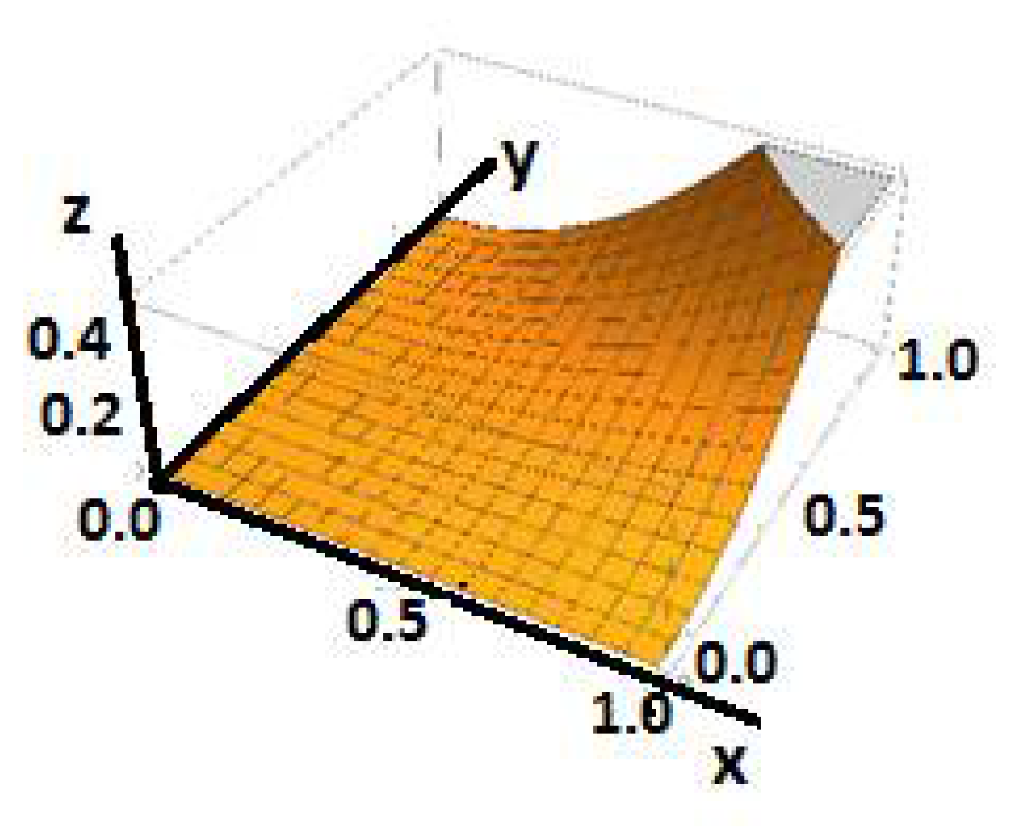
in the initial space. See Figure 1.
z = x2y2, 0 < x < 1, 0 < y < 1
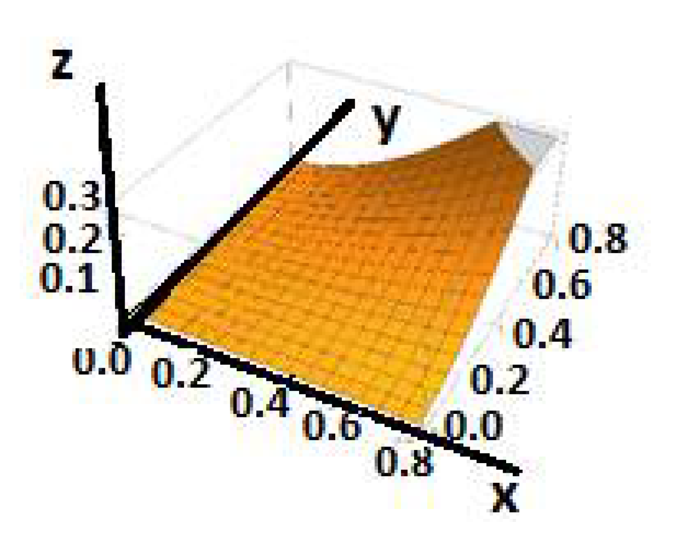
Transferring the surface into the fractional Λ-space (X, Y, Z) is defined by:
With a = b = 0, Equation (16) yields:
For γ = 0.6, the surface Z in the Λ-fractional space is defined by:
Z = 0.947X1.714Y1.714.
That surface in the Λ-fractional space is shown in Figure 2.
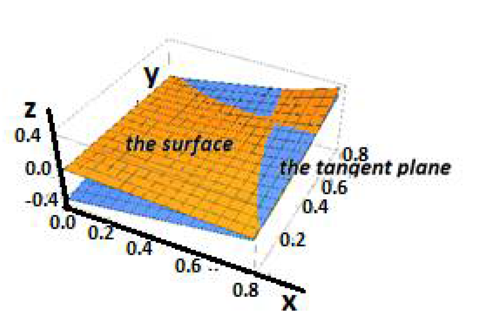
Recalling conventional differential geometry procedures, the tangent space of the surface with γ = 0.6, at the point X = Y = 0.6 is defined by:
Simplified by:
Z = 0.164 + 0.469(X − 0.6) + 0.469(Y − 0.6)
Figure 3 shows the tangent space of the surface in the Λ-fractional space.
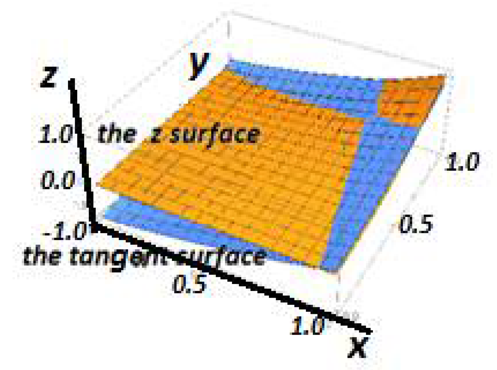
The corresponding surface in the initial space to the tangent plane in the Λ-fractional space is defined by:
The surface is shown in Figure 4.
4. The Fractional Field Theorems
The conventional field theorems are expressed by:
- a.
- Green’s theorem. Let Qx(x,y), Qy(x,y), be smooth real functions in a domain Ω, with its boundary being a smooth closed curve . Then,
Corollary: When Qx(x,y), Qy(x,y), are derived by a potential function (x,y) with the RHS of Equation (22) becomes zero. That means that the curvilinear integral along a closed smooth boundary is zero.
- b.
- Stoke’s theorem:
For a smooth vector field F defined on a simple surface Ω with the boundary , Stoke’s theorem is expressed by:
where ( denotes the scalar product.
- c.
- The Gauss’ (divergence) theorem:
For a space region Ω with a smooth surface boundary , the volume integral of the divergence of a vector field F over Ω is equal to the surface integral of F over the boundary :
Although the field theorems are valid in the fractional Λ-space, they are not necessarily valid in the initial space. Nevertheless, the results from the Λ-space may be pulled back to the initial space. The application that follows indicates the procedure.
5. Fractional Multiple Integrals and Calculus of Variations
Since, in the fractional Λ-space, everything behaves conventionally, the variations of multiple integrals follow the well-known common procedure of Weinstock [10]. Hence, for a double integral in the fractional Λ-space,
yields the extremizing function,
along with the condition,
on boundary C. Let us point out that the variational procedures presented for the fractional problems are questionable since they mix variations of fractional order with variations of the order of the variable.
6. Existence and Uniqueness Theorems of Λ-Fractional Differential Equations
To emphasize the importance of Λ-fractional analysis in various fields of mathematics, physics, mechanics, economy, etc., it is pointed out that the Λ-fractional derivative is the unique fractional derivative satisfying the prerequisites of differential topology for generating differentials. Therefore, the various theorems concerning the existence and uniqueness of solutions of differential equations may be transferred from the conventional analysis to the Λ-fractional one. The various presented equations with Riemann—Liouville or Caputo derivatives or other fractional derivatives never discuss questions such as existence and uniqueness. Similar situations take place in physics and mechanics, dealing with fractional problems without the existence of differential geometry. The Λ-fractional derivative takes care of all these hindrances.
The fundamental theorem of existence and the uniqueness theorem of ordinary differential equations [24] p. 63 may be transferred in the Λ-fractional space as follows for equations of the type:
in the Λ-fractional space, satisfying the Lipschitz condition:
which satisfies the Λ-fractional equation and reduces to Υ0 when X = X0. The solution may be transferred into the initial space through the relation:
Further, the theorem proposed by Sonia Kowalewski concerning the existence of a solution of a Λ-fractional partial differential equation is mentioned in [25], p. 49.
If G(Y) and all its Λ-derivatives are continuous for if X0 is a given number and Z0 = G(Y,0), Q0 =, and if F(X,Y,Z,G) and all its partial derivatives are continuous in the region S defined by:
then there exists a unique function Φ(X,Y) such that:
- (a)
- Φ(Χ,Υ) and all its partial derivatives are continuous in the region R defined by:
- (b)
- For all (X,Y) in R, Z = Φ(X,Y) is a solution of the equation:
- (c)
- For all values of Y in the interval , Φ(X0,Y) = G(Y).
The solution may be transferred into the initial space through the equation:
7. Linear Oscillations with Fractional Dissipation
Consider a body of mass m, moving along the axis x, with the action of an elastic spring of modulus k, and friction coefficient μm in the initial space. Then, the Λ- space is defined with the T axis corresponding to the t-axis of the initial space by:
Then, the Lagrangian is defined by:
Therefore, the equation of motion in the Λ-space is defined by:
with and the initial conditions:
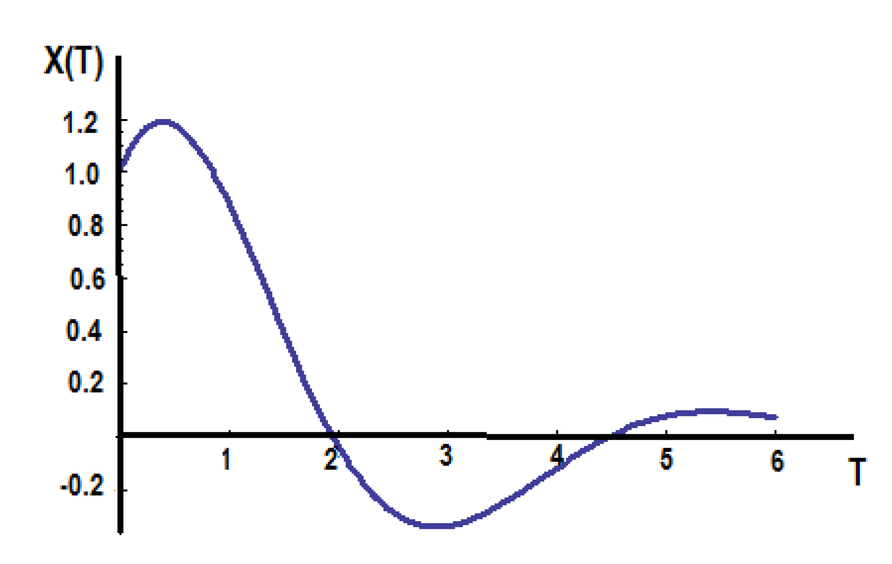
The solution to the differential equation for T > 0 is:
That solution is valid in the Λ-fractional space. For the parameters:
the solution is shown in Figure 5.
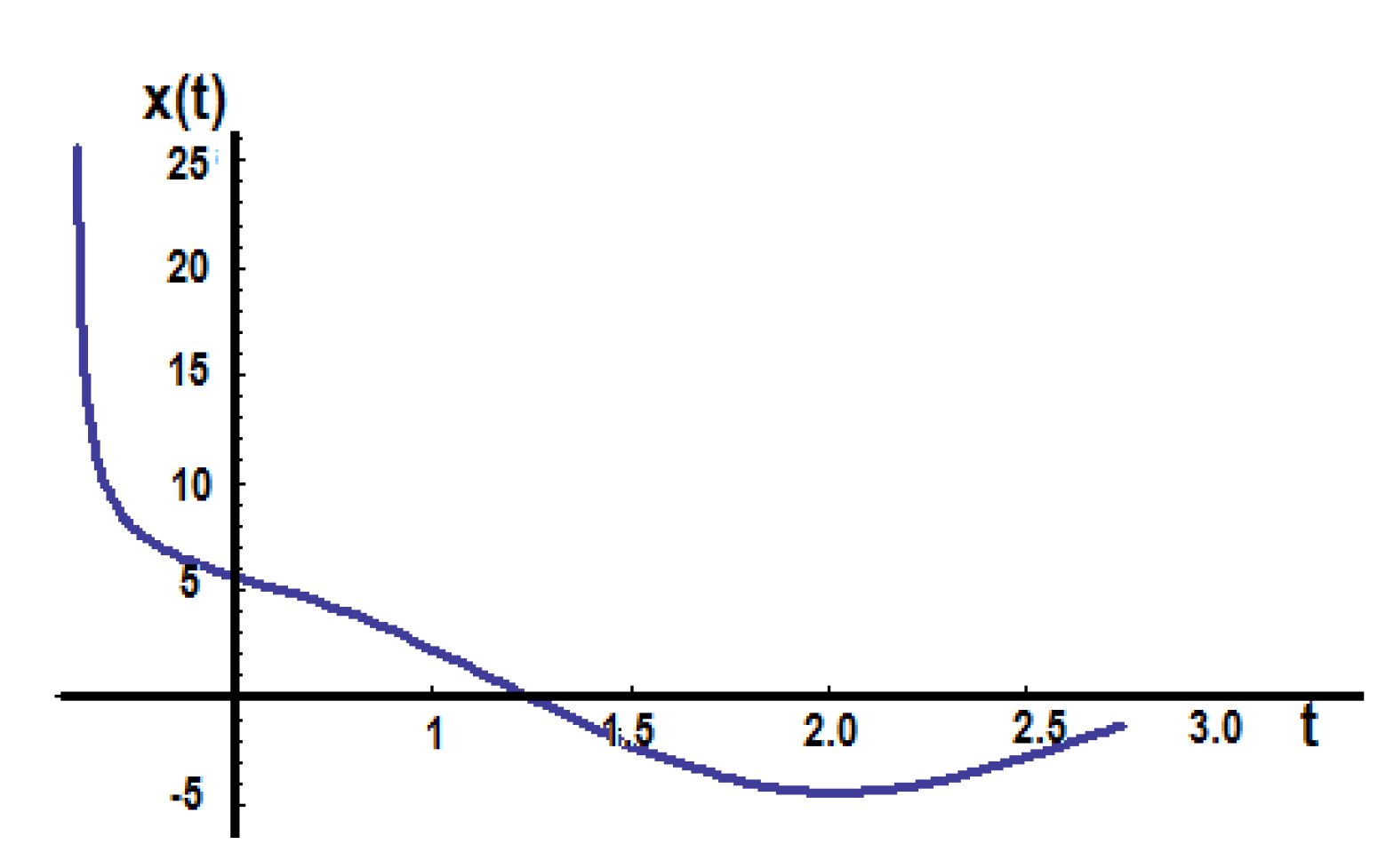
Transferring the solution to the initial space (t, x(t)), the expression of T(t) where:
should be substituted into the expression of the solution X(T), so
Then the solution x(t) in the initial space is defined by the equation:
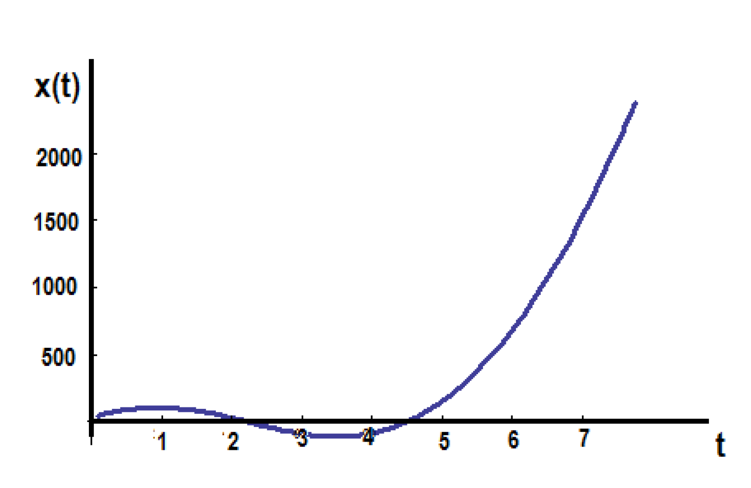
To understand the influence of the time-fractional order γ, the figure of the displacement x(t) has been computed for fractional order γ = 0.8 and is shown in Figure 7.
After a discussion of the Λ-fractional ordinary equations, the Λ-fractional partial equations will be studied in the next section.
8. The Wave Equation
Proceeding to the discussion of the wave equation:
in the Λ-space with the initial condition:
its solution is presented in Sneddon [24], p. 220. In fact, where:
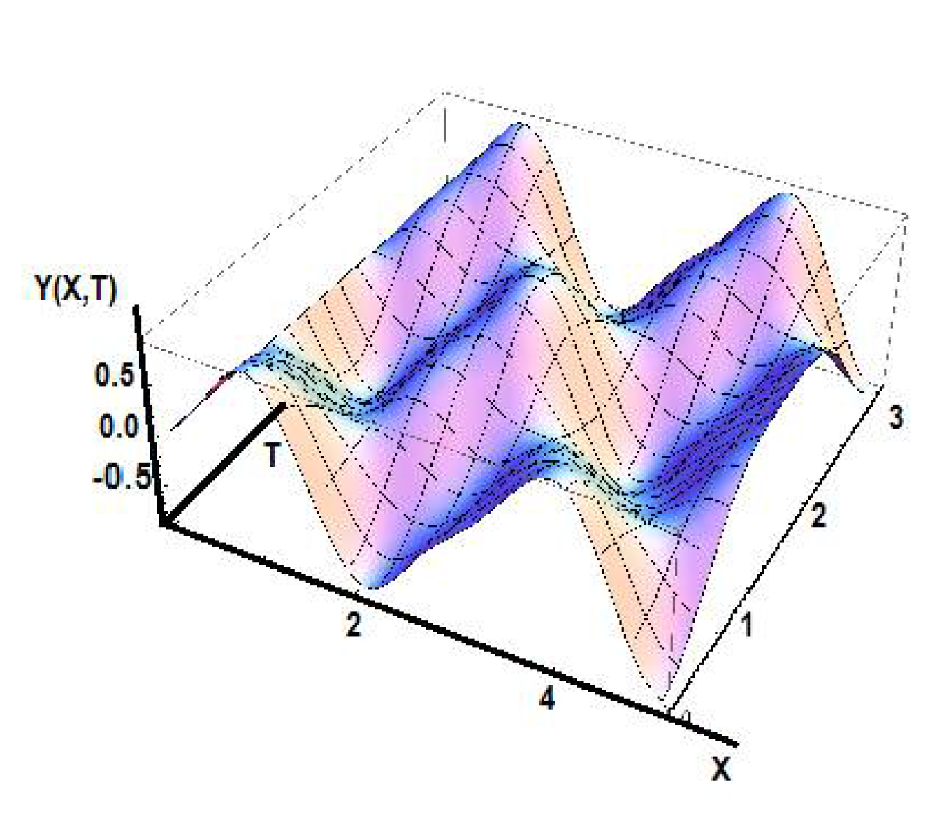
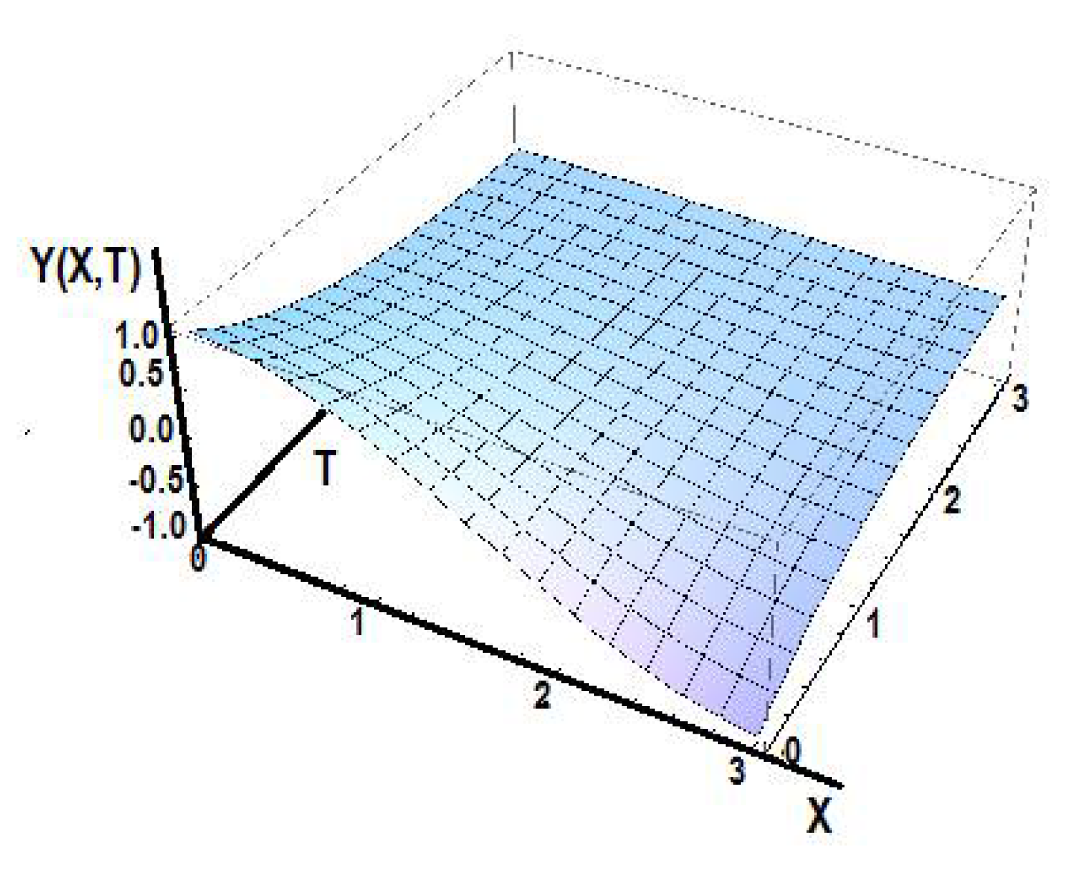
and υ(X) = 0, the solution in the Λ-space is presented by:
The Λ-fractional space should be transferred into the initial space. At this point, there are two cases. The first is the fractional time with fractional order γ1 only. The second is the additional fractional order γ2 of the space x co-ordinate to simulate the non-homogeneous media, such as porous or composite materials.
Considering homogeneous media, the solution Y(X,T) is transferred into the initial space recalling that:
Then, introducing these values into the function of Y(X,T), it is defined as:
Then, the solution of the equation y(x,t) is defined by transferring the function Y(x,t) from the Λ-fractional space to the initial one through the transformation:
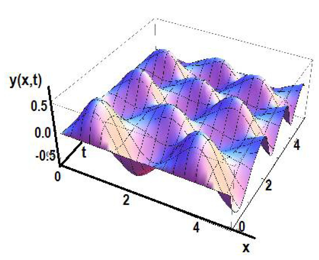
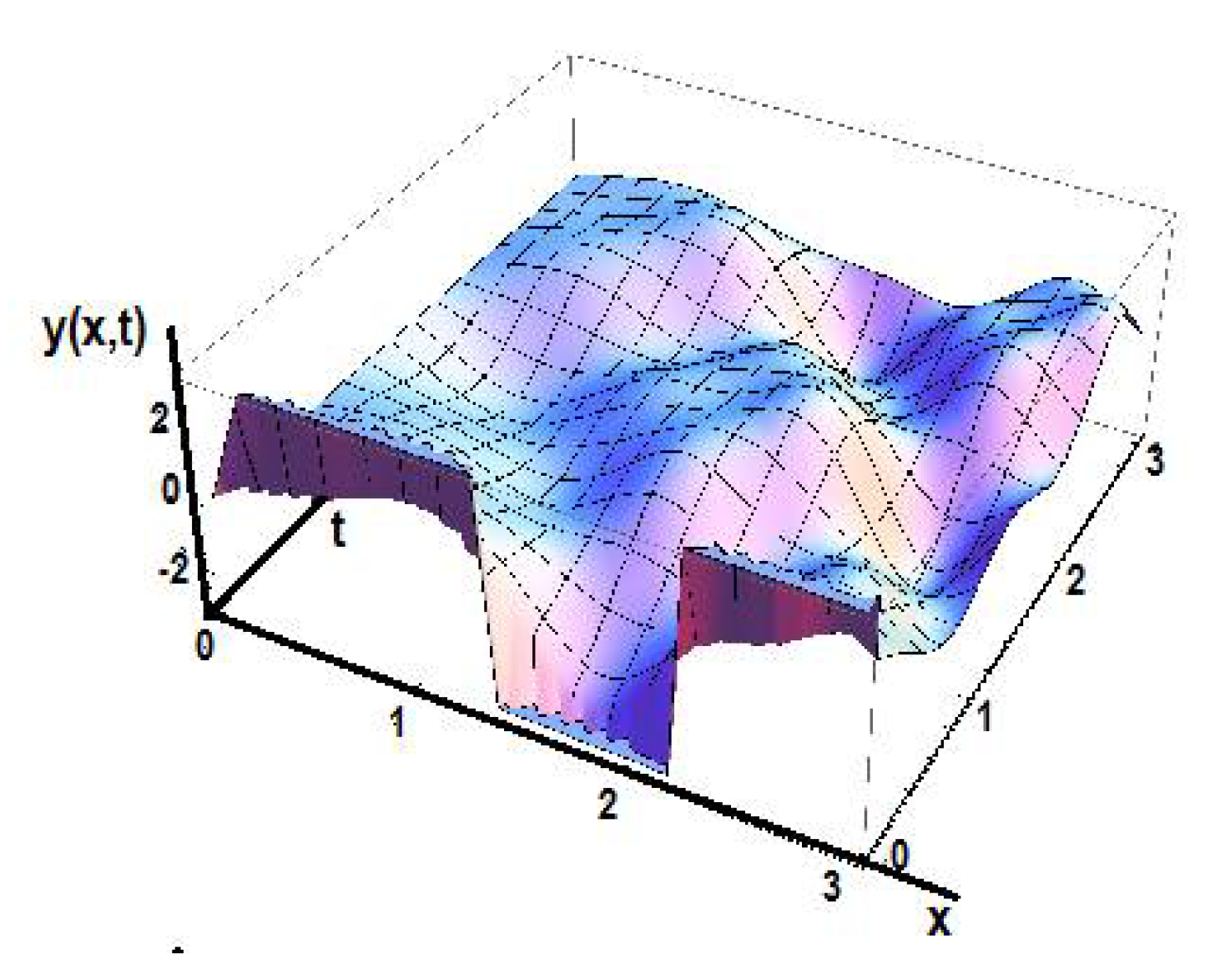
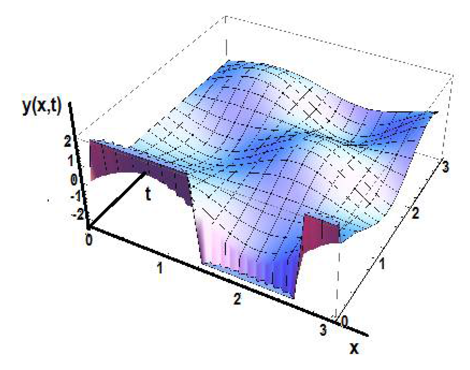
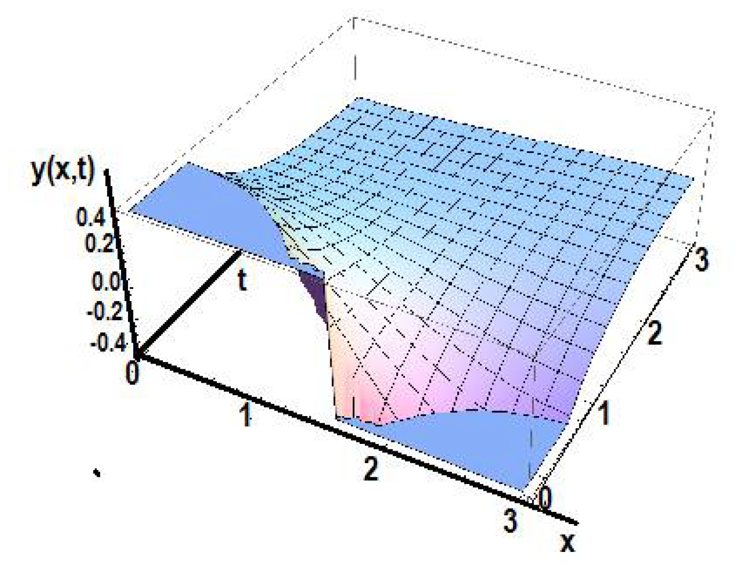
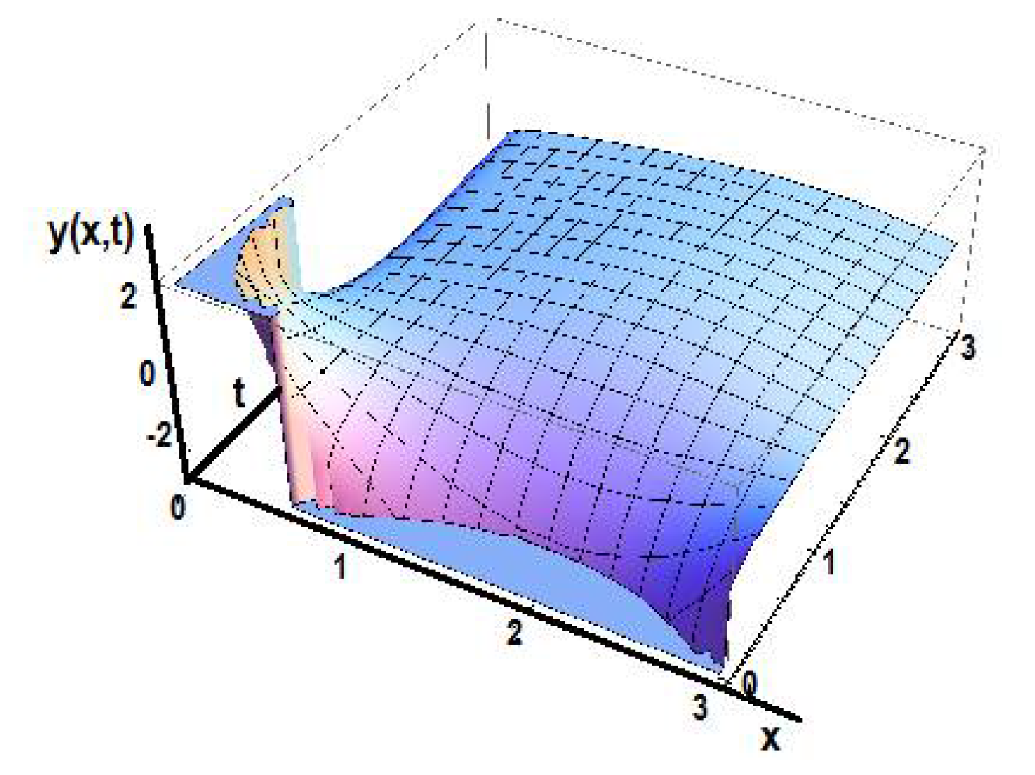
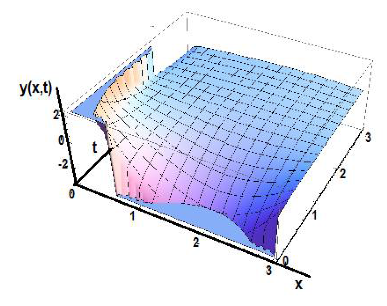
Figure 9 shows the solution of the equation in the initial space for γ1 = 0.5.
To understand the influence of the time-fractional order γ1, the solution in the initial space is presented for fractional order γ1 = 0.8 in Figure 10.
Let us proceed to the discussion of the wave equation of fractional time order γ1 with additional fractional order γ2 of the space x co-ordinate to simulate the non-homogeneous media, such as porous or composite materials.
Transferring the solution Y(X,T) into the initial space it is recalled that:
Then, introducing these values into the function of Y(X,T), it is defined:
Then, the solution of the equation y(x,t) is defined by transferring the function Y(x,t) from the Λ-fractional space to the initial through the transformation:
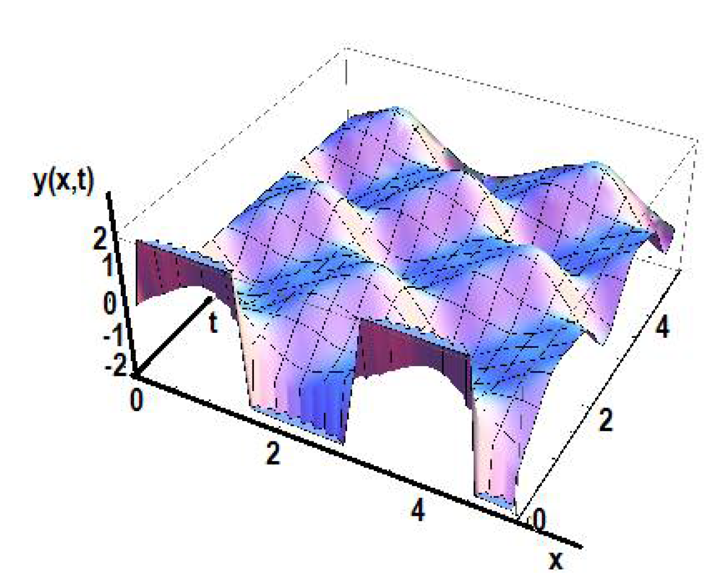
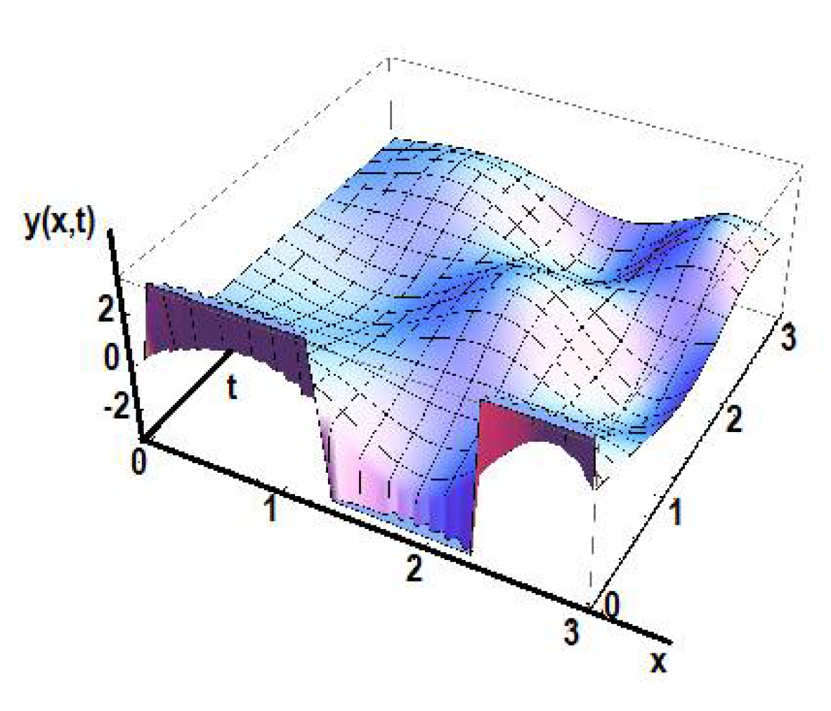
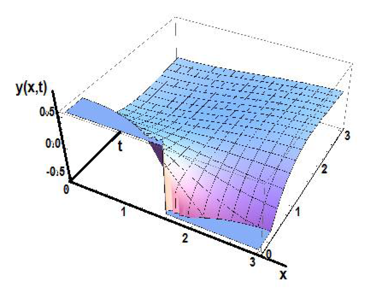
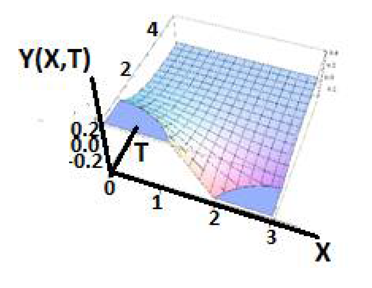
Figure 11 shows the solution of the equation in the initial space for fractional time order γ1 = 0.5 and space fractional order γ2 = 0.5 corresponding to various non-uniformities of the medium.
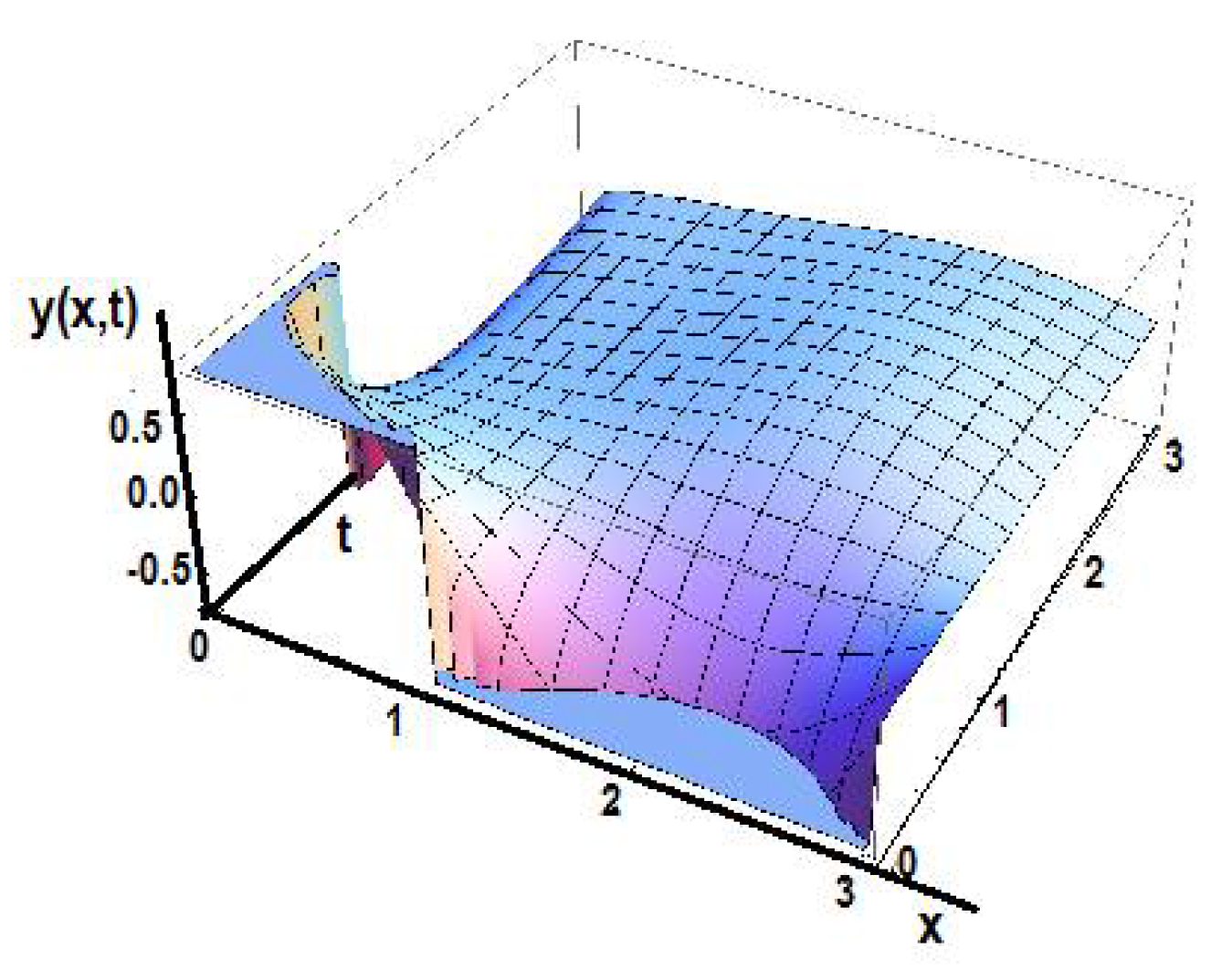
Further, the solution y(x,t) for time fractional order γ1 = 0.5 and space fractional order γ2 = 0.8 is shown in Figure 12.
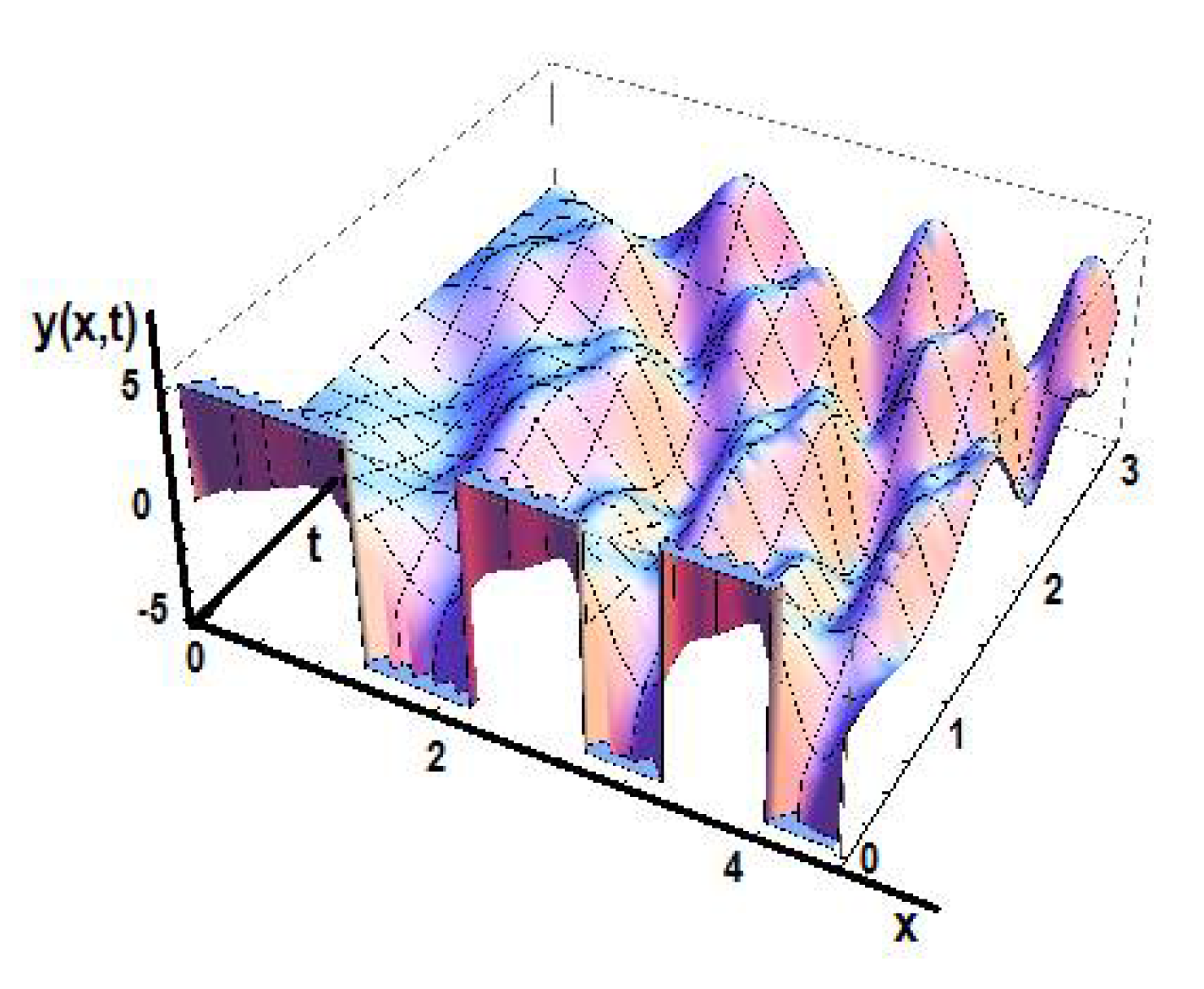
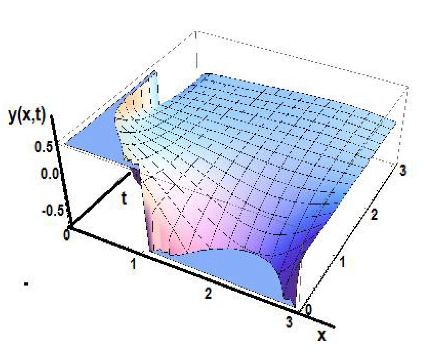
Proceeding further for the solutions with time-fractional order γ1 = 0.8, the solution y(x,t) for space-fractional order γ2 = 0.5 is shown in Figure 13.
Likewise, for the solutions with time-fractional order γ1 = 0.8, the solution y(x,t) for space-fractional order γ2 = 0.8 is shown in Figure 14.
9. The Λ-Fractional Diffusion Equation
The one-dimensional Λ-fractional diffusion equation is defined as the conventional diffusion equation in the Λ-fractional space. Indeed,
with the b.cs:
The solution to the diffusion equation is defined by (see Sneddon [24], p. 124):
First-time fractional space is considered with fractional order γ1 only. In that case,
Hence,
Transferring the solution to the initial space,
Presenting a simplified solution, the initial condition,
is considered with k = 1. The solution in the Λ-fractional space, in that case, is defined by,
Figure 15 shows the solution of the diffusion equation in the Λ-fractional space.
Hence,
Transferring the function of the solution from the Λ-fractional space to the initial space, the solution y(x,t) is defined by,
Figure 16 shows the solution of the diffusion equation for fractional order γ1 = 0.5.
Figure 17 shows the solution of the diffusion equation for fractional order γ1 = 0.8. in the initial space.
Let us proceed to the discussion of the diffusion equation of fractional time order γ1 with additional fractional order γ2 of the space x co-ordinate to simulate the non-homogeneous media, such as porous or composite materials. In that case,
Hence,
Transferring the solution to the initial space,
To simplify the algebra in transferring the solution from the Λ-fractional space to the initial one, the solution:
is considered with k = 1. It is recalled the solution in the Λ-fractional space, in that case, is defined by:
Figure 18 shows the solution of the diffusion equation in the Λ-fractional space.
Hence,
Transferring the function of the solution from the Λ-fractional space to the initial space, the solution z(x,t) is defined by:
Figure 19 shows the solution of the diffusion equation fortime fractional order order γ1 = 0.5 and space fractional order γ2 = 0.5.
Figure 20 shows the solution of the diffusion equation fortime fractional order order γ1 = 0.5 and space fractional order γ2 = 0.8.
Figure 21 shows the solution of the diffusion equation fortime fractional order order γ1 = 0.8 and space fractional order γ2 = 0.5.
Figure 22 shows the solution of the diffusion equation fortime fractional order order γ1 = 0.8 and space fractional order γ2 = 0.8.
10. Branching of the Λ-Fractional Differential Equations
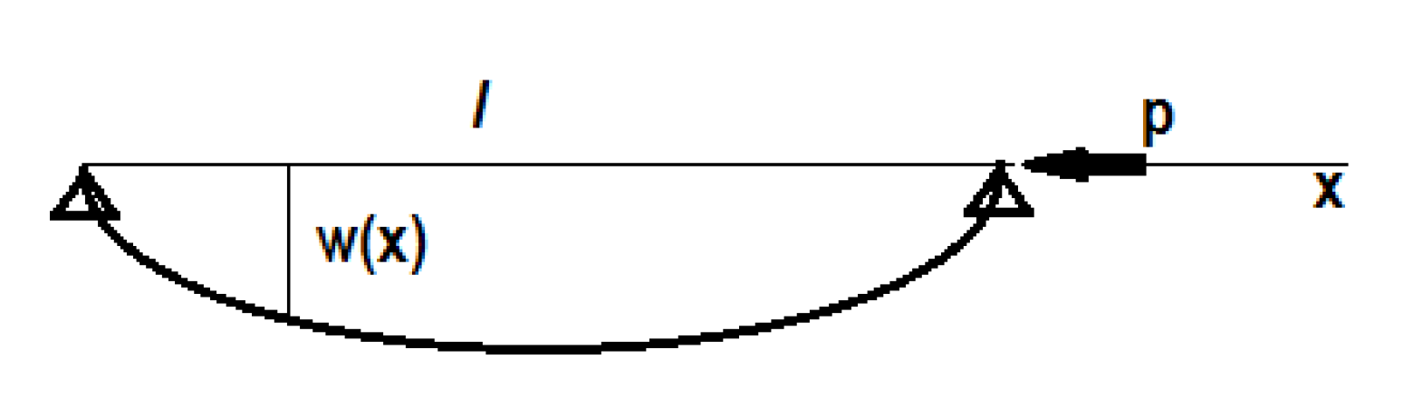
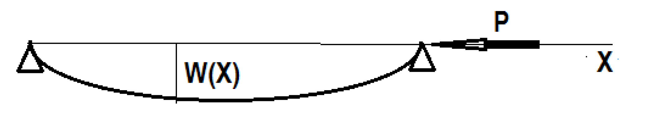
Λ-fractional analysis is applied to the branching of the Λ-fractional inextensible beam under axial load. Consider a simply supported beam with axis 0 < x < l. The axial load p is applied upon the support at x = l. The branching beam deflection is defined by w(x), see Figure 23.
The axis x in the initial space corresponds to the X axis in the Λ-fractional space where:
The length l and the axial force p are changing in the Λ-fractional space. They correspond to L and P where:
Then the free energy of the beam is expressed by:
where S is the arc length of the inextensible elastic curve of the beam, EI is the stiffness of the beam, and δL is the axial displacement of the load P applied upon the moving end of the beam. Hence, the free energy of the beam, Equation (67), is given by:
Since , the free energy function is expressed by:
The equilibrium problem is defined by the minimum of V expressed by the variational equation:
Hence, the equilibrium equation is expressed as an equation of the deflection W(S) by:
with the b.cs,
Applying branching theory (see Vainberg &Trenogin [26]) the homogeneous linear problem,
with the above b.cs, is expressed by:
with
Further, increasing the loading by:
the branching equation becomes:
According to Fredholm alternative theorem, the branching equation has a solution if,
The above branching condition defined the deflection of the branching curve as a function of the incremental axial force by:
Hence, the branching elastic curve of Equation (77) in the Λ-fractional space is defined by:
The branching elastic curve should be transferred from the Λ-fractional space to the initial space. Proceeding to define the branching elastic line in the initial space, Equation (64) connecting the two variables X and x should be pointed out. Hence, the branching equation in the Λ-fractional space expressed in variables of the initial space is defined by:
Finally, the branching equation in the initial space is defined by:
11. Conclusions
Λ-fractional differential equations have been discussed. Fractional differential equations exhibit the handicap that the well-known fractional derivatives do not correspond to differentials, since, according to differential topology, they are not real mathematical derivatives. Furthermore, fractional differential geometry may not be a source for fractional differential equations. Additionally, field theory and variational procedures may not be sources for generating fractional derivatives. The proposed Λ-fractional differential equations are compatible with all the well-known theories of differential equations in the Λ-fractional space. The various solutions may be transferred from the Λ-fractional space to the initial one. Typical Λ-fractional equations have been solved concerning oscillations, waves, diffusion, and branching problems.
Funding
This research received no external funding.
Institutional Review Board Statement
Not applicable.
Informed Consent Statement
Not applicable.
Data Availability Statement
Not applicable.
Conflicts of Interest
The authors declare no conflict of interest.
References
- Truesdell, C.; Noll, W. The non-linear field theories of mechanics. In Handbuch der Physik; Fluegge, S., Ed.; Springer: Berlin, Germany, 1965; Volume 3. [Google Scholar]
- Mandelbrot, B. The Fractal Geometry of Nature; W.H. Freeman: New York, NY, USA, 1983. [Google Scholar]
- Aharony, A. Fractals in Physics. Europhys. News 1986, 17, 41–43. [Google Scholar] [CrossRef]
- Havlin, S.; Buldyrev, S.V.; Goldberger AL’ Mantegna, R.N.; Ossadnik, S.M.; Peng, C.K.; Simons, M.; Stanley, H.E. Fractals in biology and medicine. Chaos Solitons Fractals 1995, 6, 171–201. [Google Scholar] [PubMed]
- Barnsley, M.F. Fractals Everywhere; Academic Press: Orlando, FL, USA, 1998. [Google Scholar]
- Feder, J. Fractals; Plenum Press: New York, NY, USA; London, UK, 1988. [Google Scholar]
- Eringen, A.C. Nonlocal Continuum Field Theories; Springer: New York, NY, USA, 2002. [Google Scholar]
- Leibnitz, G.W.; Letter, G.A. L’Hospital. Leibnitzen Math. Schr. 1849, 2, 301–302. [Google Scholar]
- Liouville, J. Sur le calcul des differentielles a indices quelconques. J. Ec. Polytech. 1832, 13, 71–162. [Google Scholar]
- Chillingworth, D.R.J. Differential Topology with a View to Applications; Pitman: London, UK, 1976. [Google Scholar]
- Samko, S.G.; Kilbas, A.A.; Marichev, O.I. Fractional Integrals and Derivatives: Theory and Applications; Gordon and Breach: Amsterdam, The Netherlands, 1993. [Google Scholar]
- Podlubny, I. Fractional Differential Equations (An Introduction to Fractional Derivatives, Fractional Differential Equations, Some Methods of Their Solution and Some of Their Applications); Academic Press: San Diego, CA, USA; Boston, MA, USA; New York, NY, USA; London, UK; Tokyo, Japan; Toronto, ON, Canada, 1999. [Google Scholar]
- Oldham, K.B.; Spanier, J. The Fractional Calculus; Academic Press: New York, NY, USA; London, UK, 1974. [Google Scholar]
- Lazopoulos, K.A.; Lazopoulos, A.K. On the Mathematical Formulation of Fractional Derivatives. Prog. Fract. Diff. Appl. 2019, 5, 261–267. [Google Scholar]
- Lazopoulos, K.A.; Lazopoulos, A.K. On fractional geometry of curves. Fractal Fract. 2021, 5, 161. [Google Scholar] [CrossRef]
- Lazopoulos, K.A.; Lazopoulos, A.K.; Pirentis, A. On Λ-Fractional Differential Geometry. In Proceedings of the 9th (Online) International Conference on Applied Analysis and Mathematical Modeling-Abstracts Book (ICAAMM21), Istanbul, Turkey, 11–13 June 2021. [Google Scholar]
- Lazopoulos, K.A.; Lazopoulos, A.K. On Λ-fractional Elastic Solid Mechanics. Mecc. Online 2022, 57, 775–791. [Google Scholar] [CrossRef]
- Lazopoulos, K.A.; Lazopoulos, A.K. On plane Λ-fractional linear elasticity theory. Theor. Appl. Mech. Lett. 2020, 10, 270–275. [Google Scholar] [CrossRef]
- Lazopoulos, K.A.; Lazopoulos, A.K. On fractional bending of beams with Λ-fractional derivative. Arch. App. Mech. 2020, 90, 573–584. [Google Scholar] [CrossRef]
- Lazopoulos, K. On Λ-fractional analysis & Mechanics. Axioms 2022, 11, 85. [Google Scholar]
- Di Paola, M.; Failla, G.; Sumelka, W. New prospects in non-conventional modeling of solids and structures. Meccanica 2022, 57, 751–755. [Google Scholar] [CrossRef]
- Patnaik, S.; Sidhardh, S.; Sempeloti, F. Displacement-driven approach to non-local elasticity. Eur. J. Mech. A/Solids 2022, 92, 104434. [Google Scholar] [CrossRef]
- Shaat, M.; Ghanvaloo, E.; Fazelzadeh, S. Review on nonlocal continuum mechanics: Physics, material applicability, and mathematics. Mech. Mater. 2020, 150, 103587. [Google Scholar] [CrossRef]
- Ince, E.L. Ordinary Differential Equations; Dover: New York, NY, USA, 1959. [Google Scholar]
- Sneddon, I. Elements of Partial Differential Equations; McGraw-Hill Book Company, Inc.: New York, NY, USA; Toronto, ON, Canada; London, UK, 1957. [Google Scholar]
- Vainberg, M.; Trenogin, V. Theory of Branching of Solutions of Nonlinear Equations; Nauka: Moscow, Russia, 1969. [Google Scholar]
Figure 1.
The surface z in the initial space.

Figure 2.
The surface Z in the Λ-fractional space.

Figure 3.
The tangent space of the surface in the Λ-fractional space.

Figure 4.
The surface with its tangent surface at the point (x = y = 0.8106) at the initial space.

Figure 5.
The solution X(T) in the Λ-fractional space.

Figure 6.
The solution x(t) in the initial space for γ = 0.5.

Figure 7.
The solution x(t) in the initial space for γ = 0.8.

Figure 8.
Solution of Y(X,T) in the Λ-space.

Figure 9.
The solution of the wave solution y(x,t) for γ1 = 0.5.

Figure 10.
The solution in the initial space y(x,t) for γ1 = 0.8.

Figure 11.
The solution y(x,t) in the initial space for γ1 = 0.5 and γ2 = 0.5.

Figure 12.
The solution y(x,t) in the initial space for γ1 = 0.5 and γ2 = 0.8.

Figure 13.
The solution y(x,t) in the initial space for γ1 = 0.8 and γ2 = 0.5.

Figure 14.
The solution y(x,t) in the initial space for γ1 = 0.8 and γ2 = 0.8.

Figure 15.
The solution of the diffusion equation in the Λ-space.

Figure 16.
The solution of the diffusion equation in the initial space for fractional order γ1 = 0.5.
Figure 16.
The solution of the diffusion equation in the initial space for fractional order γ1 = 0.5.

Figure 17.
The solution of the diffusion equation in the initial space for fractional order γ1 = 0.8.
Figure 17.
The solution of the diffusion equation in the initial space for fractional order γ1 = 0.8.

Figure 18.
The solution of the diffusion eq. in the Λ-space.

Figure 19.
The solution of the diffusion equation in the initial space for time fractional order γ1 = 0.5 and space fractional order γ2 = 0.5.
Figure 19.
The solution of the diffusion equation in the initial space for time fractional order γ1 = 0.5 and space fractional order γ2 = 0.5.

Figure 20.
The solution of the diffusion equation in the initial space for time fractional order γ1 = 0.5 and space fractional order γ2 = 0.8.
Figure 20.
The solution of the diffusion equation in the initial space for time fractional order γ1 = 0.5 and space fractional order γ2 = 0.8.

Figure 21.
The solution of the diffusion equation in the initial space for time fractional order γ1 = 0.8 and space fractional order γ2 = 0.5.
Figure 21.
The solution of the diffusion equation in the initial space for time fractional order γ1 = 0.8 and space fractional order γ2 = 0.5.

Figure 22.
The solution of the diffusion equation in the initial space for time fractional order γ1 = 0.8 and space fractional order γ2 = 0.8.
Figure 22.
The solution of the diffusion equation in the initial space for time fractional order γ1 = 0.8 and space fractional order γ2 = 0.8.

Figure 23.
Branching curve in the initial plane (x,w(x)).

Figure 24.
Branching curve in the Λ-space (X,W(X)).

Publisher’s Note: MDPI stays neutral with regard to jurisdictional claims in published maps and institutional affiliations. |
© 2022 by the author. Licensee MDPI, Basel, Switzerland. This article is an open access article distributed under the terms and conditions of the Creative Commons Attribution (CC BY) license (https://creativecommons.org/licenses/by/4.0/).
Share and Cite
MDPI and ACS Style
Lazopoulos, K.A. On Λ-Fractional Differential Equations. Foundations 2022, 2, 726-745. https://0-doi-org.brum.beds.ac.uk/10.3390/foundations2030050
AMA Style
Lazopoulos KA. On Λ-Fractional Differential Equations. Foundations. 2022; 2(3):726-745. https://0-doi-org.brum.beds.ac.uk/10.3390/foundations2030050
Chicago/Turabian StyleLazopoulos, Konstantinos A. 2022. "On Λ-Fractional Differential Equations" Foundations 2, no. 3: 726-745. https://0-doi-org.brum.beds.ac.uk/10.3390/foundations2030050