
Caputo Fractional Evolution Equations in Discrete Sequences Spaces


Calle Pedro Cerbuna 12, Departamento de Matemáticas, IUMA, Universidad de Zaragoza, 50009 Zaragoza, Spain
*
Author to whom correspondence should be addressed.
†
These authors contributed equally to this work.
Foundations 2022, 2(4), 872-884; https://0-doi-org.brum.beds.ac.uk/10.3390/foundations2040059
Submission received: 30 August 2022
/
Revised: 20 September 2022
/
Accepted: 26 September 2022
/
Published: 11 October 2022
(This article belongs to the Special Issue Recent Advances in Fractional Differential Equations and Inclusions)
Abstract
:In this paper, we treat some fractional differential equations on the sequence Lebesgue spaces with . The Caputo fractional calculus extends the usual derivation. The operator, associated to the Cauchy problem, is defined by a convolution with a sequence of compact support and belongs to the Banach algebra . We treat in detail some of these compact support sequences. We use techniques from Banach algebras and a Functional Analysis to explicity check the solution of the problem.
1. Introduction
The main objective of this paper is to study the following semidiscrete Cauchy differential equation
where B is a convolution operator in the discrete variable, i.e.,
and the sequence b belongs to the Banach algebra A first example is the one-dimensional discrete Laplacian, which is defined by where denotes the discrete Dirac measure given by the Kronecker delta, i.e., if and 0 in other case. Equation (1) is usually called the lattice diffusion equation or the semidiscrete heat equation.
These classes of equations have received a wide interest in the mathematical literature in the last years. They appear in diverse areas of knowledge. For example, in probability theory, the function of (1) with expresses the probability that a continuous-time symmetric random walk arrives at point n at time ([1], [Section 4]). In chemical physics, (1) describes the flow of a liquid in an infinite row of tanks where two neighbors are always connected [2], [Section 3]. Another amazing application takes place in transport theory. Equation (1) expresses the dynamics of an infinite chain of cars, each of them being coupled to its two neighbors. The function is the displacement of car n at time t from its equilibrium point ([3], [Example 1]). Quite recently, Slavik [4] studied the asymptotic behavior of solutions of (1) when , showing that a bounded solution approaches the average of the initial values if the average exists. In the case that in (2), we obtain the forward difference operator and then the Equation (2) describes the semidiscrete transport system, treated recently by Abadias et al. in [5].
Other interesting references, such as [6,7], present fundamental solutions for (1) and the second-order semidiscrete equation
when is the fractional power of discrete fractional Laplacian. In the particular case of [7], the authors apply operator theory techniques and some of the properties of the Bessel functions to obtain a theory of uni-parametric operators (-semigroups and cosine operators) generated by and on the Lebesgue space . Moreover, note that the fractional forward difference operator has been treated in [5] where the maximum and comparison principles in the context of Fourier Analysis are shown.
However, there is no attempt (to the best of our knowledge) to present explicitly fundamental solutions of the general Equation (1) on the sequence space for instead of on the sequence space for ([8]).
The main technique in this paper is that we apply our knowledge from Banach algebras and Functional Analysis to fractional differential systems. This useful approach that we follow in this paper, allows us to obtain a completely new point of view. We prove results by introducing this new method and describing both the qualitative and quantitative behavior of the fundamental solutions of (1) in a unified way.
More generally, and to present simultaneously our studies of the subdiffusive and superdiffusive cases connected to Equations (1) and (3), in this article, we deal with the representation of the fundamental solutions for the following semidiscrete system:
in case and
in case In both cases, B is the convolution operator defined for and is a real number. The symbol denotes the Caputo fractional derivative of order
The paper is organized as follows. In the first section, we introduce the main results about the Banach algebras and, in particular, about the spaces and . In the second section, we consider some particular finite difference operators in , mainly
for . Finally, we present Theorem 6 where we include the representation of the fundamental solutions for semidiscrete Caputo fractional differential equations.
This paper contains part of the results included in the Master Thesis of the first author, entitled “Semigrupos y operadores coseno generados por operadores de diferencias finitas en espacios de sucesiones de Lebesgue”, Universidad de La Rioja, (2021).
Notation The usual set numbers , , , and are used. We write as the unit circumference (or also called torus) and . The Dirac measures and are if and for . We denote by the indicator function on set I (i.e., if and if ).
Furthermore, and are the Bessel functions and the usual Hermite polynomials; is the Gamma function, the Wright function and the Mittag-Leffler function.
Given X Banach space, is the dual of Banach space and the set of linear bounded operators on X; given , we write is the adjoint of the operator A.
2. A Banach Algebra Framework
Given , we recall that the Banach spaces are formed by infinite sequences such that
We remind that the natural embeddings , for , and that the dual of is identified with where for and if .
In the case that and ), we define
From Young’s Inequality, it follows that and . We denote by defined by for . The element g is called the symbol of the convolution operator .
Note that is a commutative Banach algebra with identity that we denote by . We observe that and, in general, for . As usual, we write and for .
The Gelfand transform associated to , is the -transform, , (or Taylor series), where
We recall that the resolvent set of f, denoted as
and the spectrum of f, .
In what follows, we apply the general theory of Functional Analysis and commutative Banach Algebra as framework. In the following theorem, we collect some results that will be of our interest, see [9].
Theorem 1.
The following properties hold:
- (i)
- The spectrum is compact and, consequently, homeomorphic to the unit complex circle,
- (ii)
- and
- (iii)
- The algebra is a semi-simple regular Banach algebra and the -transform is injective.
- (iv)
- and
- (v)
- Given and the linear convolution operator for for . Then,
We recall that the Banach algebra is formed by bi-infinite sequences such that
Given , the product in the algebra is the usual convolution product given by
Note that is also a commutative Banach algebra with identity and for . The Gelfand transform associated to , is the Fourier series (or discrete Fourier transform), , where
The spectrum is homeomorphic to the unit torus, and ([8], (Theorem 2.1)).
Definition 1.
Given we define the vector-valued Mittag-Leffler function, , by
Note that
The set is the connected component of in the set of regular elements in ([9], Theorem 6.4.1).
Now, we remind the usual terminology in semigroup theory: an element is called the generator of the entire group given by the exponential function . The cosine function is expressed by its generator in terms of Mittag-Leffer function , see [10], (Sections 3.1 and 3.14). Moreover, the Laplace transform of an entire group or a cosine function is connected with the resolvent of its generator as follows:
see, for example, ([10], p. 213).
Example 1.
For , we have that
In particular, and are generated by .
In the next proposition, we present some technical properties of these Mittag-Leffler functions in the Banach algebra . As usual, we consider vector-valued integration (in the sense of Bochner) in the Banach space , see, for example, ([11], Section 1.2).
Proposition 1.
For and , we have that
- (i)
- (ii)
- in particular, and for .
- (iii)
- .
- (iv)
- The following Laplace transform formula holdsfor
Theorem 2.
Given and , we define the operator ) by
- (i)
- and .
- (ii)
Proof. (i) It is clear that and . Now, take , and for . Then,
for . We conclude that .
(ii) Now, take . Then, and . We conclude that . □
3. Some Finite Difference Operators in
Sequences of compact support, i.e., elements in the set
are an important case of finite difference operators. In such a case, the discrete Fourier Transform of is a trigonometric polynomial
It is interesting to observe that if , then . This follows immediately from .
Definition 2.
For with , we define the following operators
- 1.
- .
- 2.
- .
- 3.
- .
- 4.
- .
- 5.
- .
- 6.
- .
- 7.
- .
for and for .
The above operators are often used in the context of a numerical analysis. The operators and ∇ are connected with the Euler scheme of approximation. The discrete Laplacian is the second-order central difference approximation for the second-order derivative. The double Laplacian, the operator , is introduced in Bateman’s seminar paper ([12], Page 506), to treat the equations of Born and Karman on crystal lattices in vibration. Other operators , and are also considered in [12].
To consider the action of these operators in , we study these operators as elements in the Banach algebra as Theorem 2 shows. Operators , ∇, and have been studied in detail in ([8], Theorem 3.2, 3.3, 3.4 and 3.5). In the following subsections, we treat , and .
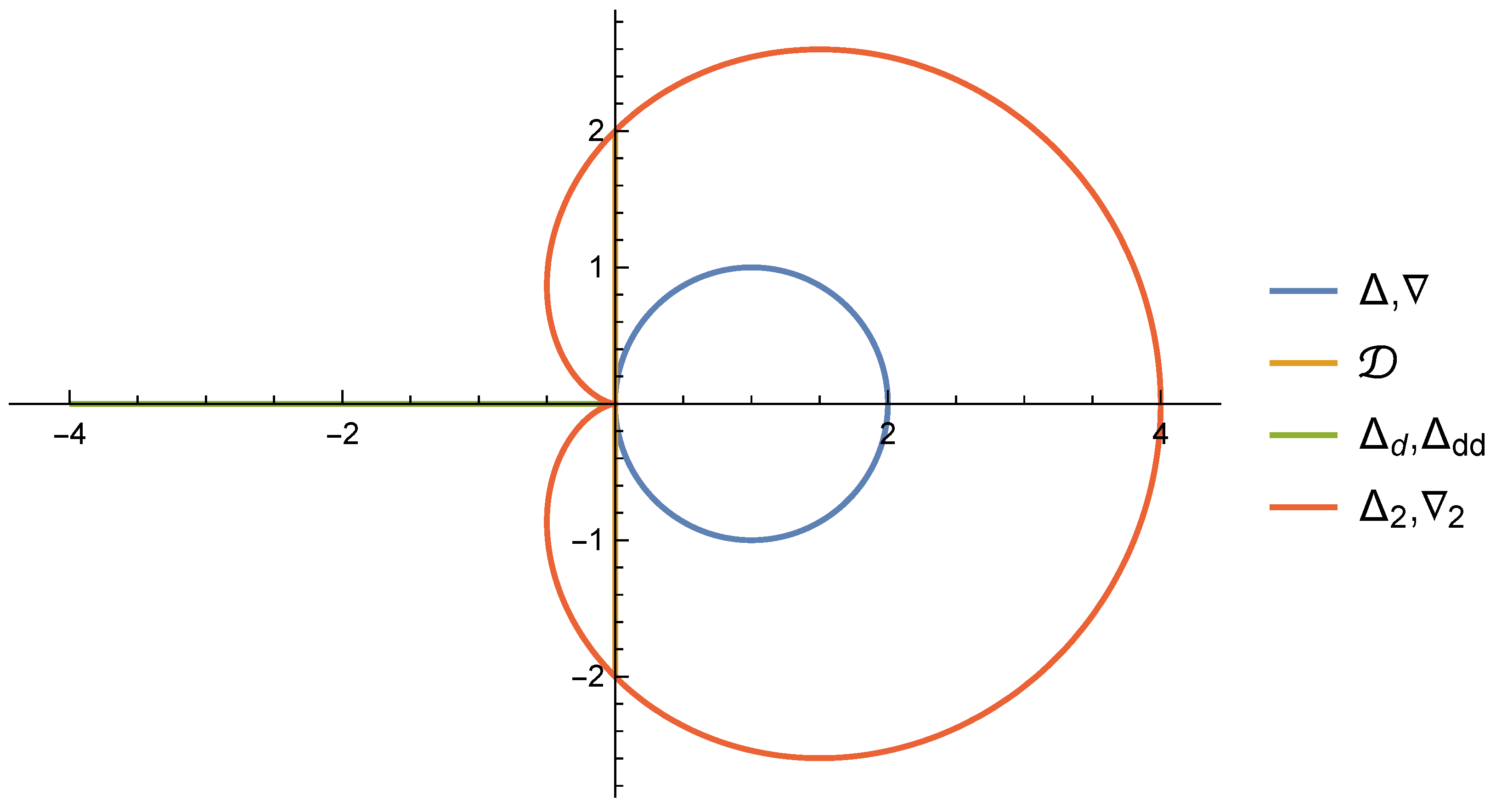
In Table 1, we collect some basic results of the finite difference operators given in Definition 2. In Figure 1, we also plot the spectrum for these finite difference operators.
3.1. The Operator
This operator is a finite difference operator of order 1 defined by . We present some of these properties in the next theorem.
Theorem 3.
The operator with , has the following properties.
- (i)
- The norm of a is equal to 2, .
- (ii)
- The discrete Fourier transform of a is given by with .
- (iii)
- The spectrum of a is .
- (iv)
- The group generated by is , , and , with and .
- (v)
- For ,
Proof. Items (i) and (ii) are straightforward. To show (iii), we have that
We define for a while with by . Note that
where we have applied the generating function of modified Bessel function of the first kind with , see, for example, [13], [Appendix].
We apply the discrete Fourier transform to obtain
with . As the discrete Fourier transform is injective, we conclude that and the item (iv) is proved.
Finally, to show item (v), we have that
where we have applied ([14], Formula 6.623) for and . By analytic prolongation, we extend the equality for . □
3.2. The Operator
The operator is a finite difference operator of order 2. Note that . In the next theorem, we present some properties of .
Theorem 4.
The operator with verifies the following properties.
- (i)
- The norm of a is equal to 4, .
- (ii)
- The discrete Fourier transform with .
- (iii)
- The spectrum of a in is equal to .
- (iv)
- The group generated by a isand for .
- (v)
- The cosine function .
Proof. Items (i), (ii) and (iii) are similar to items (i), (ii) and (iii) in Theorem 3. Now, we define con by where is the Hermite polynomial. First, we check that ,
We calculate the discrete Fourier transform of
where we have applied ([14], Formula 8.951), for . As the discrete Fourier transform is injective, we conclude that for .
To calculate the cosine function generated by a, we apply ([10], Example 3.14.15)
and we conclude the proof.□
3.3. The Operator
In this subsection, we treat the finite difference operator of order 2, defined by . Note that e . We present some basic properties of operator .
Theorem 5.
The operator with has the following properties.
- (i)
- The norm of a in is equal to 4, .
- (ii)
- The discrete Fourier transform for .
- (iii)
- The spectrum of a in is equal to .
- (iv)
- The group generated by a is given byand , for .
- (v)
- The cosine function .
Proof. We skip the proof of items (i), (ii) and (iii). To show (iv), we define for . As in Theorem 4, and
for . We conclude that for . As , we apply again ([10], Example 3.14.15), to obtain the cosine function generated by a. □
Remark 1.
The connection between semigroups and cosine functions is given by the so-called Weierstrass formula,
for , see, for example, ([10], Theorem 3.14.17). In the case that we apply the Weierstrass formula in the conditions of Theorems 4 and 5 to obtain the well-known formula
see, for example, ([14], Formula 3.462(4)).
4. Fundamental Solution for Semidiscrete Evolution Equations
In this section, we consider the operator , with , , and . We obtain an explicit representation of solutions for the following time/space fractional evolution equation:
Here, is real number. We recall that denotes the Caputo fractional derivative given by
for and
for . For and , we consider the usual first- and second-order derivation. Note that
however,
see, for example, [15,16].
The main result in this section is the following Theorem. The function (with ) is the vector-valued Mittag-Leffler function given in Definition 1. A similar result was stated in the Banach space in ([8], Theorem 5.1).
Theorem 6.
Let , and be such that, for each , and with
Proof. We show part (ii) in the case . Part (i) or are proved in a similar way. We prove the result in several steps.
Now, taking Laplace’s transformation to (13), we have:
By inverse Laplace transform, see identity (9), we obtain
We apply Proposition 1 (ii) to obtain
for and .
Step 2. Now, we prove uniqueness. Suppose that the system (5) has two solutions and with the same initial values , , and write . Then, v is a solution of the following ODE
Due to the above ordinary differential equation having its unique solution and that the function zero is a solution, we conclude that . As the -transform is injective, we conclude that for every and . Hence, .
Step 3. By Proposition 1 (i), we obtain that
for and . Because , we conclude that
and the solution for . □
Remark 2.
Now, we may shortly treat the behavior of the solution when tends to natural parameter, i.e., . For simplicity, we only present the homogeneous case, . In the case that , the solution of Equation (4) tends to semigroup family operators , and when , the solution of Equation (5),
tends to the well-known solution of second-order Cauchy problem, expressed in terms of cosine function and sine function generated by b, see ([10], Corollary 3.14.8).
However, in the case that , the solution of Equation (5) converges to
as in the scalar case. We remark that this function is the solution of the following first-order modified Cauchy problem
for . This natural fact is connected with the interpolation property of the Caputo fractional differentiation, see (12).
The fundamental solution for Equations (4) and (5) is given by taking as initial values and . In the case ( is the wave equation), a second fundamental solution is given by and , see ([17], Remark 3.2).
As a corollary of Theorems 2 and 6 is the following subordination theorem for fundamental solutions. This result extends ([17], Corollary 3.5) in the space .
We denote by the entire Wright function defined by
where is a complex path which starts and ends at and rounds the origin once counterclockwise. The Wright function is a known special function which has appeared in a wide variety of different contexts, for example, it is used for models in stochastic processes, see [18]. The proof of the next corollary is similar to ([8], Corollary 5.3), and we leave for the reader.
5. Conclusions and Future Work
In this paper, we have considered Caputo fractional differential equations in the sequence Lebesgue spaces with . The associate operator is given by a convolution with a sequence in the Banach Algebra which belongs to . We use techniques from the Functional Analysis, such as the Guelfand theory in Banach algebra, to obtain more information about the problem. We calculate the explicit solution in terms of Mittag-Leffer functions. Some particular cases (sequences of compact support) of finite difference operators are treated in detail.
An interesting problem to address in the future is to consider these techniques in the continuous case. We may study these Caputo fractional differential equations in and .
Author Contributions
Conceptualization, A.M. and P.J.M.; methodology, A.M. and P.J.M.; software, A.M. and P.J.M.; investigation, A.M. and P.J.M.; writing, A.M. and P.J.M.; funding acquisition, A.M. and P.J.M. All authors have read and agreed to the published version of the manuscript.
Funding
This research received no external funding.
Institutional Review Board Statement
This study did not require ethical approval.
Informed Consent Statement
Not applicable.
Data Availability Statement
Not applicable.
Acknowledgments
The authors have been partially supported by ProjectID2019-105979GBI00, DGI-FEDER, of the MCEI and Project E48-20R, Gobierno de Aragón, Spain.
Conflicts of Interest
The authors declare no conflict of interest.
References
- Friesl, M.; Slavik, A.; Stehlik, P. Discrete-space partial dynamic equations on time scales and applications to stochastic processes. Appl. Math. Lett. 2014, 37, 86–90. [Google Scholar] [CrossRef]
- Slavik, A. Mixing problems with many tanks. Am. Math. Mon. 2013, 120, 806–821. [Google Scholar] [CrossRef] [Green Version]
- Feintuch, A.; Francis, B. Infinite chains of kinematic points. Autom. J. IFAC 2012, 48, 901–908. [Google Scholar] [CrossRef]
- Slavik, A. Asymptotic behavior of solutions to the semidiscrete diffusion equation. Appl. Math. Lett. 2020, 106, 106392. [Google Scholar] [CrossRef]
- Abadias, L.; de León-Contreras, M.; Torrea, J.L. Non-local fractional derivatives. Discrete and continuous. J. Math. Anal. Appl. 2017, 449, 734–755. [Google Scholar] [CrossRef] [Green Version]
- Ciaurri, O.; Lizama, C.; Roncal, L.; Varona, J.L. On a connection between the discrete fractional Laplacian and superdiffusion. Appl. Math. Lett. 2015, 49, 119–125. [Google Scholar] [CrossRef]
- Lizama, C.; Roncal, L. Hölder-Lebesgue regularity and almost periodicity for semidiscrete equations with a fractional Laplacian. Discr. Cont. Dyn. Syst. Ser. A 2018, 38, 1365–1403. [Google Scholar] [CrossRef] [Green Version]
- González-Camus, J.; Lizama, C.; Miana, P.J. Fundamental solutions for semidiscrete evolution equations via Banach algebras. Adv. Differ. Equ. 2021, 2021, 35. [Google Scholar] [CrossRef] [PubMed]
- Larsen, R. Banach Algebras: An Introduction; Marcel Dekker: New York, NY, USA, 1973. [Google Scholar]
- Arendt, W.; Batty, C.; Hieber, M.; Neubrander, F. Vector-Valued Laplace Transforms and Cauchy Problems; Monographs in Mathematics; Birkhäuser-Verlag: Basel, Switzerland, 2001; Volume 96. [Google Scholar]
- Sinclair, A.M. Continuous Semigroups in Banach Algebras; London Mathematical Society, Lecture Note Series; Cambridge University Press: Cambridge, UK, 1982; Volume 63. [Google Scholar]
- Bateman, H. Some simple differential difference equations and the related functions. Bull. Am. Math. Soc. 1943, 49, 494–512. [Google Scholar] [CrossRef] [Green Version]
- Ciaurri, O.; Gillespie, T.A.; Roncal, L.; Torrea, J.L.; Varona, J.L. Harmonic analysis associated with a discrete Laplacian. J. d’Anal. MathéMatique 2017, 132, 109–131. [Google Scholar] [CrossRef]
- Gradshteyn, I.S.; Ryzhik, I.M. Table of Integrals, Series and Products, 7th ed.; Elsevier: Amsterdam, The Netherlands; Academic Press: Burlington, MA, USA; San Diego, CA, USA; London, UK, 2007. [Google Scholar]
- Bazlekova, E.G. Fractional Evolution Equations in Banach Spaces; Technische Universiteit: Eindhoven, The Netherlands, 2001. [Google Scholar]
- Gorenflo, R.; Mainardi, F. Parametric Subordination in Fractional Diffusion Processes. In Fractional Dynamics, Recent Advances; Klafter, J., Lim, S.C., Metzler, R., Eds.; World Scientific: Singapore, 2012; pp. 229–263. [Google Scholar]
- González-Camus, J.; Keyantuo, V.; Lizama, C.; Warma, M. Fundamental solutions for discrete dynamical systems involving the fractional Laplacian. Math. Meth. Appl. Sci. 2019, 42, 1–24. [Google Scholar] [CrossRef]
- Gorenflo, R.; Luchko, Y.; Mainardi, F. Analytical properties and applications of the Wright function. Fract. Calc. Appl. Anal. 1999, 2, 383–414. [Google Scholar]
Figure 1.
Spectrum of finite difference operators in .


Table 1.
Finite difference operators in .
| A | a | |||
|---|---|---|---|---|
| 2 | ||||
| ∇ | 2 | |||
| 2 | ||||
| 4 | ||||
| 4 | ||||
| 4 | ||||
| 4 |
Publisher’s Note: MDPI stays neutral with regard to jurisdictional claims in published maps and institutional affiliations. |
© 2022 by the authors. Licensee MDPI, Basel, Switzerland. This article is an open access article distributed under the terms and conditions of the Creative Commons Attribution (CC BY) license (https://creativecommons.org/licenses/by/4.0/).
Share and Cite
MDPI and ACS Style
Mahillo, A.; Miana, P.J. Caputo Fractional Evolution Equations in Discrete Sequences Spaces. Foundations 2022, 2, 872-884. https://0-doi-org.brum.beds.ac.uk/10.3390/foundations2040059
AMA Style
Mahillo A, Miana PJ. Caputo Fractional Evolution Equations in Discrete Sequences Spaces. Foundations. 2022; 2(4):872-884. https://0-doi-org.brum.beds.ac.uk/10.3390/foundations2040059
Chicago/Turabian StyleMahillo, Alejandro, and Pedro J. Miana. 2022. "Caputo Fractional Evolution Equations in Discrete Sequences Spaces" Foundations 2, no. 4: 872-884. https://0-doi-org.brum.beds.ac.uk/10.3390/foundations2040059