Article

Propagation of Surface Waves in a Rotating Coated Viscoelastic Half-Space under the Influence of Magnetic Field and Gravitational Forces

by
Ali Mubaraki
1,
Saad Althobaiti
2 and
Rahmatullah Ibrahim Nuruddeen
3,*
1
Department of Mathematics and Statistics, College of Science, Taif University, P.O. Box 11099, Taif 21944, Saudi Arabia
2
Department of Sciences and Technology, Ranyah University College, Taif University, P.O. Box 11099, Taif 21944, Saudi Arabia
3
Department of Mathematics, Faculty of Science, Federal University Dutse, Dutse P.O. Box 7156, Nigeria
*
Author to whom correspondence should be addressed.
Submission received: 4 November 2021 / Revised: 19 November 2021 / Accepted: 25 November 2021 / Published: 2 December 2021
(This article belongs to the Special Issue Recent Advances in Computational Physics with Fractional Application)

Abstract

:
The present manuscript focuses on the study of surface wave propagation in a rotating coated viscoelastic half-space and its response to external forces comprised of the magnetic field and gravitational forces. A celebrated normal mode analysis procedure is adopted as the methodology of interest for its high level of efficiency in the literature. The analytically obtained frequency equation is analyzed for certain scenarios of curiosity, in addition to the determination of the resulting displacements and stresses. Moreover, certain physical data of relevance with the viscoelasticity index of unity are considered for the numerical simulations. As for the findings, the presented graphical illustrations showed that both the magnetic field and rotation positively accelerated the dispersion of surface waves in the coated half-space, while the obtained approximate fields in the half-space are found to be oscillatory as they steadily move towards the limiting point.

1. Introduction

The propagation of waves in coated and layered elastic solids has received substantial attention in the past and in recent times due to its vast collection of applications. Various science and engineering applications have been identified to heavily rely on the elasticity subject. This subject is governed by Hooke’s law and the famous Newton’s second law of motion, among others, for appropriately modeling different wave propagation problems in diverse elastic media and structures. Furthermore, engineering fields including aerospace, civil, seismic, and marine, to mention a few, are known to enjoy many contributions from the elasticity theory (see [1,2,3,4,5,6]). A more particular concern in this study is the modeling and analysis of coated half-space. From an engineering viewpoint, the coated structures have a wide range of advantages and arise in many areas such as civil, mechanical, manufacturing, medical, and pharmaceutical, to mention a few. Additionally, coated media and structures are not different from layered structures as they have similar geometric and mechanical bases. However, the coatings are primarily used to save the structural surfaces from corrosive and other external causative harms. They are also aimed at improving adhesion, resistance, and wettability, in addition to sound control [7,8,9,10,11]. Another area where coating is applicable is in the construction of medical biomaterial devices in which coatings are utilized to lessen the mechanical loads on the surface of the implant, for instance [12,13].
Furthermore, many studies have been carried out in recent times with regard to the influence of other factors affecting the propagation of elastic waves in various structures. These factors include the presence of internal and external forces such as the magnetic field force, gravitational force, and thermal heating effect, to mention a few; one can equally think of other known factors such as external loads, initial stress, elastic foundation, rotational effects, porosity presence, dislocation, and cracks, among others (see [14,15,16,17,18,19,20,21,22,23,24,25,26] and the references therein). In line with this, the identification and determination of the motion’s resulting vibrational displacements, stresses, and frequency equation, as well as the various fields of the respective external effects that result from the coined thermoelasticity, magnetoelasticity, or poroelasticity, have forced many mathematicians and researchers to source for different mathematical techniques. The techniques are computational, analytical, and asymptotic to appropriately analyze the governing model. We mention here certain methods in [27,28,29,30,31,32,33,34,35,36,37,38,39], where such methodologies were utilized, including the integral transform approach, normal mode analysis approach, harmonic solution approach, eigenvalues approach, and some numerical schemes, among others.
However, the current manuscript focuses on the study of the propagation of elastic surface waves in a rotating coated higher-order viscoelastic half-space amidst the influence of certain external forces. The external forces under analysis include both the magnetic field force and the gravitational force, in addition to which the entire structure is presumed to be in a rotating orientation. The celebrated normal mode analysis procedure is set to be utilized as the methodology, having demonstrated a high level of efficiency in the literature. Thus, the resulting generalized frequency equation will be determined and analyzed for certain scenarios of curiosity, in addition to the determination of the corresponding displacements and stresses in the coated rotating viscoelastic half-space. Furthermore, certain physical data of relevance with a particular viscoelasticity index are considered for the numerical simulation, which is graphically illustrated to portray the influence of the magnetic field intensity and rotation on the propagation and dispersion of elastic surface waves in the governing structure. Moreover, we arrange the present manuscript in the following manner: the basic governing equations of motion in the presence of certain external forces are given in Section 2, while Section 3 gives the formulation of the problem and its related agreed boundary and interfacial conditions. Section 4 utilizes the normal mode approach to tackle the formulated problem. Furthermore, Section 5 gives the resulting frequency equation and its analysis, while Section 6 gives the numerical results and discussion, and Section 7 is reserved for the conclusion.

2. Basic Equations

The celebrated equation of motion in an elastic isotropic homogeneous medium with body forces F i and gravity G i is given via Einstein summation by [28,29,30,31,32,33,34]
σ i j , j + F i + G i = ρ u ¨ i , i = j = 1 , 2 , ,
where σ i j is given by
σ i j = λ ε k k δ i j + 2 μ ε i j , ε i j = 1 2 u i , j + u j , i ,
where, in the above equations, u i is the displacement, u ¨ i = 2 u t 2 is the acceleration, ρ is the density, σ i j is the stress–strain relation, ε i j is the strain–displacement relation, λ and μ are the Lame’s elastic constants, and δ i j the Kronecker delta.
In addition, if the body forces F i are considered to be due to the magnetic force from the linearized Maxwell equations, the force takes the following form [27,28,32,34]:
F i = μ 0 H 0 2 e , i ϵ 0 μ 0 u ¨ i ,
where μ 0 is the magnetic permeability, ϵ 0 is the electric field permeability, H 0 is the magnetic field intensity, and e = u j j for j = 1 , 2 , is the dilatational strain. Moreover, the gravitational field force G i is considered based on Biot’s definition [40,41]. Finally, when the media are assumed to be in moving frame with only centripetal acceleration, the acceleration in Equation (1) becomes [29,32,34]
u ¨ i = u ¨ i Ω u i ,
where Ω is the angular velocity.

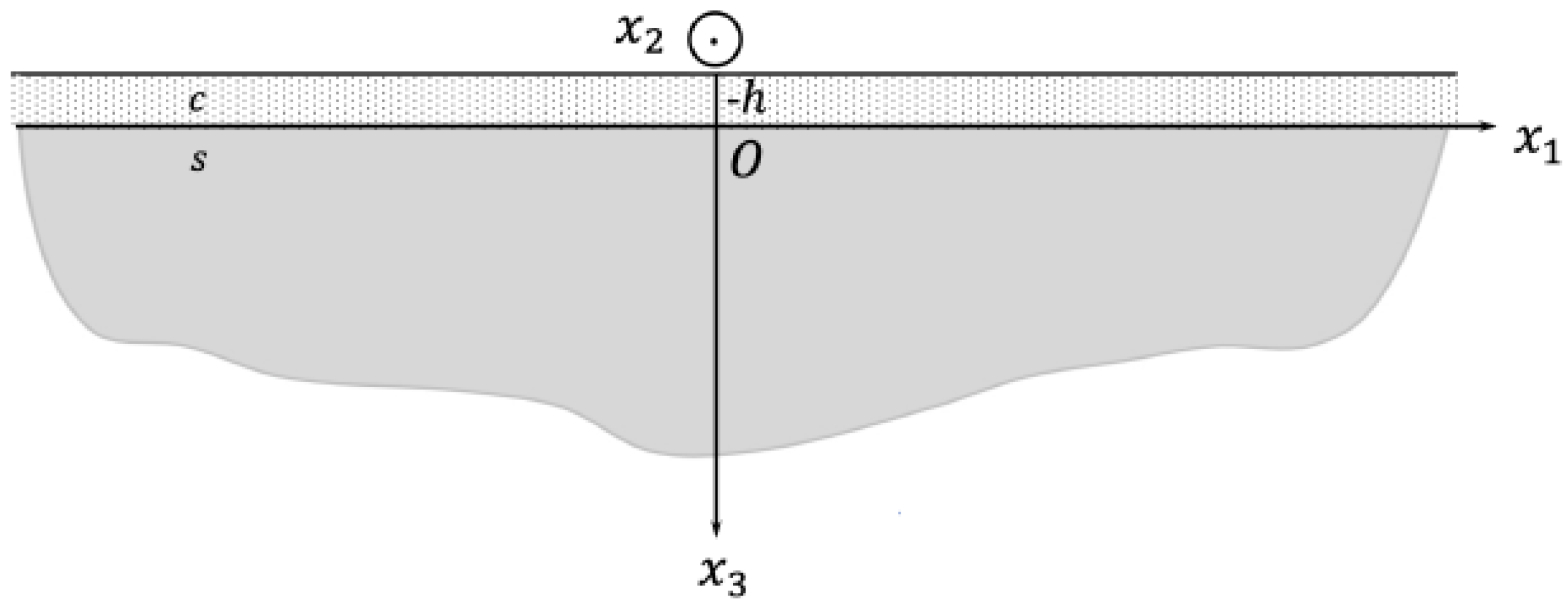
3. Problem Formulation

Consider a thin coating of constant thickness h occupying the region h x 3 0 , perfectly joint with an elastic half-space, employing the domain < x 1 , x 2 < and 0 x 3 < (see Figure 1; this Figure is taken from Mubaraki, 2021 [42]).
The entire structure is further assumed to be under the influence of magnetic field and gravitational forces, in addition to being assumed to be in a rotating frame of reference. Therefore, the governing isotropic plane equation of motions under these effects in the x 1 x 3 -plane and u = ( u 1 , 0 , u 3 ) takes the following form from the above given basic equation:
σ 11 , 1 q + σ 13 , 3 q + μ 0 H 0 2 ( u 1 , 11 q + u 3 , 31 q ε 0 μ 0 u ¨ 1 q ) + ρ q g u 3 , 1 q = ρ q ( u ¨ 1 q Ω 2 u 1 q ) , q = c , s ,
σ 31 , 1 q + σ 33 , 3 q + μ 0 H 0 2 ( u 1 , 13 q + u 3 , 33 q ε 0 μ 0 u ¨ 3 q ) ρ q g u 1 , 1 q = ρ q ( u ¨ 3 q Ω 2 u 3 q ) , q = c , s ,
where
σ i j q = λ q ε k k q δ i j + 2 μ q ε i j q , ε i j q = 1 2 ( u i , j q + u j , i q ) , i = j = 1 , 3 ,
where u 1 = u 1 ( x 1 , x 3 , t ) , u 3 = u 3 ( x 1 , x 3 , t ) are the in-plane displacements, μ q and λ q are elastic constants, and ρ q are the densities for q = c , s , where c stands for the coating, s stands for the half-space, and g is the gravity. Additionally, H 0 is the magnetic field intensity, ε 0 is the electric permeability, and μ 0 is the magnetic permeability, while Ω = ( 0 , Ω , 0 ) is the angular velocity due to rotation.
Moreover, the half-space is assumed to be viscoelastic in nature of higher-order m [27,43,44]. That is, the elastic constants μ s and λ s take the following form:
μ s = μ 1 n t n , λ s = λ 1 n t n , n = 1 , 2 , , m .
Furthermore, we prescribe the following mechanical boundary condition on the face of the coating at x 3 = h :
( a ) σ 13 c + τ 13 c = 0 , ( b ) σ 33 c + τ 33 c = 0 ,
and the following interfacial conditions between the coating and the half-space at x 3 = 0 are as follows:
( c ) u 1 c = u 1 s , ( d ) u 3 c = u 3 s , ( e ) σ 13 c + τ 13 c = σ 13 s + τ 13 s , ( f ) σ 33 c + τ 33 c = σ 33 s + τ 33 s .
where τ i j q is the linearized electromagnetic stress tensor due the presence of the magnetic field given by
τ i j q = μ 0 H 0 ( H i h j + H j h i H k h k δ i j ) , i = j = 1 , 3 , q = c , s ,
of which
τ 13 q = 0 , and τ 33 q = μ 0 H 0 2 ( u 1 , 1 + u 3 , 3 ) , q = c , s ,
where the magnetic field vector H i is defined as H i = ( H 0 + h i ) δ i 2 , where H 0 is the magnetic field intensity, and h i is the perturbed magnetic field that is considered to be h i = u k , k [27].

4. Problem Solution

This section determines the solution of the formulated problem by utilizing the normal node analysis method. This method gives harmonic wave solutions in both regions with the propagating wave number and phase speed being fixed. The method is far better than the widely used integral transform methods, where the inversion process normally poses difficulties.
Now, in trying to express the governing equations given in Equations (5) and (6) in component form, we make use of the relations given in Equation (7) to obtain
σ 13 q = μ q ( u 1 , 3 q + u 3 , 1 q ) = σ 31 q , σ 11 q = λ q u 3 , 3 q + ( λ q + 2 μ q ) u 1 , 1 q , σ 33 q = λ q u 1 , 1 q + ( λ q + 2 μ q ) u 3 , 3 q ,
such that the governing equations become
( λ q + 2 μ q + μ 0 H 0 2 ) u 1 , 11 q + ( λ q + μ q + μ 0 H 0 2 ) u 3 , 13 q + μ q u 1 , 33 q = ( ε 0 μ 0 2 H 0 2 + ρ q ) u ¨ 1 q + ρ q ( g u 3 , 1 q Ω 2 u 1 q ) ,
( λ q + 2 μ q + μ 0 H 0 2 ) u 3 , 33 q + ( λ q + μ q + μ 0 H 0 2 ) u 1 , 13 q + μ q u 3 , 11 q = ( ε 0 μ 0 2 H 0 2 + ρ q ) u ¨ 3 q + ρ q ( g u 1 , 1 q Ω 2 u 3 q ) ,
for q = c , s .
Now, employing the following potential functions U q and V q , the above equations of the forms
u 1 q = U , 1 q + V , 3 q , u 3 q = U , 3 q V , 1 q , q = c , s ,
and the equations in the coating take the following forms:
( c c 1 2 + χ c 1 ) 2 U c = ( 1 + χ c 2 ) U ¨ c + g V , 1 c Ω 2 U c , c c 2 2 2 V c = ( 1 + χ c 2 ) V ¨ c g U , 1 c Ω 2 V c ,
while those of the half-space take the following forms:
c s 1 2 t n 2 U s + χ s 1 2 U s = ( 1 + χ s 2 ) U ¨ s + g V , 1 s Ω 2 U s , n = 1 , 2 , , m , c s 2 2 t n 2 V s = ( 1 + χ s 2 ) V ¨ s g U , 1 s Ω 2 V s , n = 1 , 2 , , m ,
where t n = n t n for n = 1 , 2 is due to the viscoelastic nature of the half-space, and 2 = 2 x 2 + 2 y 2 is the Laplacian operator, while c q 1 2 and c q 2 2 are given by
c c 1 2 = λ c + 2 μ c ρ c , c c 2 2 = μ c ρ c , c s 1 2 = λ 1 + 2 μ 1 ρ s , c s 2 2 = μ 1 ρ s ,
and χ q 1 and χ q 2 together with χ q 3 are given by
χ q 1 = μ 0 H 0 2 ρ q , χ q 2 = ε μ 0 2 H 0 2 ρ q , χ q 3 = λ q ρ q , q = c , s ,
where c q 1 2 and c q 2 2 for q = c , s are the longitudinal and transverse speeds in the corresponding regions.
Furthermore, we make use of the potential functions U and V defined in Equation (16) to re-express the boundary conditions given in Equations (9) and (10). Therefore, the boundary conditions on the face of the coating at x 3 = h become
( a ) V , 33 c V , 11 c + 2 U , 13 c = 0 , ( b ) χ c 3 ( U , 11 c + V , 13 c ) + c c 1 2 ( U , 33 c V , 13 c ) + χ c 1 2 U c = 0 ,
and the interfacial conditions at x 3 = 0 now become
( c ) U , 1 c + V , 3 c = U , 1 s + V , 3 s , ( d ) U , 3 c V , 1 c = U , 3 s V , 1 s , ( e ) μ c ( V , 33 c V , 11 c + 2 U , 13 c ) = μ 1 t n ( V , 33 s V , 11 s + 2 U , 13 s ) , ( f ) ρ c ( χ c 3 ( U , 11 c + V , 13 c ) + c c 1 2 ( U , 33 c V , 13 c ) + χ c 1 2 U c ) = ρ s ( χ s 3 t n ( U , 11 s + V , 13 s ) + c s 1 2 t n ( U , 33 s V , 13 s ) + χ s 1 2 U s ) .
Therefore, considering x 1 to be the direction of the propagation, we now assume the following solutions in the respective layers of the media:
U q ( x 1 , x 3 , t ) = M q ( x 3 ) e i k ( x 1 c t ) , q = c , s , V q ( x 1 , x 3 , t ) = N q ( x 3 ) e i k ( x 1 c t ) , q = c , s ,
where k and c are the dimensional wave number and phase speed, respectively, such that ω = k c , where ω is the dimensional frequency.
Now, substituting the above solutions into Equations (17) and (18), we obtain the following respective solutions:
l 1 M c ( x 3 ) + l 2 N c ( x 3 ) = 0 , l 3 M c ( x 3 ) + l 4 N c ( x 3 ) = 0 ,
l 5 M s ( x 3 ) + l 6 N s ( x 3 ) = 0 , l 7 M s ( x 3 ) + l 8 N s ( x 3 ) = 0 ,
where l y for y = 1 , 2 , , 8 are given in Appendix A. Moreover, one can equivalently express Equations (24) and (25) as follows:
l 1 l 2 0 0 l 3 l 4 0 0 0 0 l 5 l 6 0 0 l 7 l 8 M c ( x 3 ) N c ( x 3 ) M s ( x 3 ) N s ( x 3 ) = 0 0 0 0 ,
of which the nontrivial solutions exist if the determinant of the differential coefficient matrix vanishes, that is,
( l 2 l 3 l 1 l 4 ) ( l 6 l 7 l 5 l 8 ) = 0 ,
or simply splitting the characteristic equations for each layer as follows:
a 1 ( D 2 ) 2 + a 2 D 2 + a 3 = 0 ,
b 1 ( D 2 ) 2 + b 2 D 2 + b 3 = 0 ,
where a 1 , a 2 , a 3 , b 1 , b 2 , and b 3 are given in Appendix B.
Finally, the solutions in the coating layer are thus obtained as follows:
U c ( x 1 , x 3 , t ) = j = 1 4 A j e α j x 3 + i k ( x 1 c t ) , V c ( x 1 , x 3 , t ) = j = 1 4 ξ j A j e α j x 3 + i k ( x 1 c t ) ,
and the solutions in the half-space layer for x 3 are thus obtained as follows:
U s ( x 1 , x 3 , t ) = j = 1 2 B j e β j x 3 + i k ( x 1 c t ) , V s ( x 1 , x 3 , t ) = j = 1 2 η j B j e β j x 3 + i k ( x 1 c t ) ,
where A j for j = 1 , 2 , , 4 and B j for j = 1 , 2 are constants to be determined, and α j for j = 1 , 2 , , 4 and β j for j = 1 , 2 are the roots of Equations (28) and (29), respectively, given by
α 1 , 2 = ± 1 2 a 2 + a 2 2 4 a 1 a 3 a 1 , α 3 , 4 = ± 1 2 a 2 2 4 a 1 a 3 a 2 a 1 ,
and
β 1 = 1 2 b 2 + b 2 2 4 b 1 b 3 b 1 , β 2 = 1 2 b 2 2 4 b 1 b 3 b 2 b 1 ,
Additionally, ξ j and η j in Equations (30) and (31) are determined as follows:
ξ j = i g k c c 2 2 k 2 v c 2 2 χ c 2 + 1 + α j 2 k 2 + Ω 2 , η j = i g k Ω 2 + c s 2 2 k 2 v s 2 2 χ s 2 + 1 + ( i c k ) n β j 2 k 2 ,
where v lq 2 = c 2 c x q 2 , q = c , s , and x = 1 , 2 , are the ratios of the phase speed to the respective regions’ speeds.
However, for the sake of numerical simulation, we set B j = 1 in Equation (31) to determine A j for j = 1 , 2 , 3 , 4 from the prescribed transformed boundary conditions in Equations (21) and (22) through solving the resulting system of algebraic equations.

5. Frequency Equation

Next, we determine the frequency equation, also called the dispersion relation of the formulated problem by utilizing the prescribed transformed boundary conditions given in terms of potential functions in Equations (21) and (22). Thus, in doing so, we obtain the following homogeneous system of equations:
a 11 a 12 a 13 a 14 a 15 a 16 a 21 a 22 a 23 a 24 a 25 a 26 a 31 a 32 a 33 a 34 a 35 a 36 a 41 a 42 a 43 a 44 a 45 a 46 a 51 a 52 a 53 a 54 a 55 a 56 a 61 a 62 a 63 a 64 a 65 a 66 A 1 A 2 A 3 A 4 B 1 B 2 = 0 0 0 0 0 0 ,
where the entries for the matrix a i j are given in Appendix C.
Furthermore, the determinant of the coefficient matrix given in Equation (35) is said to vanish in order to have the non-trivial solution of the system; that is,
| A i j | 6 × 6 = 0 .
Lastly, the resulting determinant of the dispersion coefficient matrix is the aiming generalized frequency equation or dispersion relation found above.

Special Cases of the Frequency Equation

Here, we analyze the obtained frequency equation in Equation (36) for some special and particular cases of interest. These cases include the absence of the external excitations or forces (and effects), a case of a viscoelastic half-space only, and the situation of welded half-spaces.
I. Absence of excitations
A swift case of interest would be the absence of external excitations or forces (and effects). Thus, the frequency equation given in Equation (36) corresponds to a situation when all the external forces and effects under consideration are zero; that is, the viscoelasticity is assumed to be of order zero; the magnetic field intensity is zero, H 0 = 0 ; the gravitational force is zero, g = 0 ; and finally, the rotation is zero, Ω = 0 .
II. Viscoelastic half-space
Yet another case of interest would be the absence of the coating; that is, the layer above that half-space of thickness h is considered to be zero in this case, h = 0 . Thus, the problem reduces to just a half-space problem such that 0 x 3 < . Furthermore, we obtain two additional scenarios associated with this case as follows.
(a) Traction-free end
Now, if the half-space in the presence of the prescribed external forces, rotation, and viscoelasticity is considered to have a traction-free surface at h = 0 , then the obtained frequency equation in Equation (36) reduces to the following:
b 11 b 12 b 21 b 22 = 0 ,
of which, when the external forces and rotation are assumed to be zero, the above frequency equation satisfies the following Rayleigh-wave equation [23]:
2 c 2 c s 2 2 2 = 4 1 c 2 c s 1 2 1 c 2 c s 2 2 .
(b) Fixed end
Equally, if the half-space in the presence of the prescribed external forces, rotation, and viscoelasticity is considered to have a displacement-free surface at h = 0 , then the obtained frequency equation in Equation (36) reduces to the following:
c 11 c 12 c 21 c 22 = 0 ,
and further reduces to the following when the external forces, rotation, and viscoelasticity are eliminated:
1 c 2 c s 1 2 1 c 2 c s 2 2 = 1 ,
Note that the entries b i j and c i j in Equations (37) and (39) are respectively given in Appendix D.
II. Welded half-spaces
Another case of interest would be the frequency equation of the welded half-spaces. This happens when the thickness of the coating is extended to negative infinity, that is, h . Thus, the obtained frequency equation in Equation (36) reduces to
a 31 a 32 a 35 a 36 a 41 a 42 a 45 a 46 a 51 a 52 a 55 a 56 a 61 a 62 a 65 a 66 = 0 ,
where the entries a i j are given in Appendix A. It is worth mentioning here that the two positive roots from α j for j = 1 , 2 , , 4 are considered, with already negative roots of β j for j = 1 , 2 . Moreover, when the external forces and effects under consideration are zero, including the viscoelasticity index, the above-reduced frequency equation further reduces to
ρ s c c 2 2 1 c 2 c c 1 2 1 c 2 c c 2 2 2 c s 2 4 1 c 2 c s 1 2 1 c 2 c s 2 2 + c 2 c s 1 2 1 c 2 c s 1 2 c 2 c s 2 2 1 c 2 c s 2 2 = ρ c c s 2 2 1 c 2 c s 1 2 1 c 2 c s 2 2 2 c c 2 4 1 c 2 c c 1 2 1 c 2 c c 2 2 + c 2 c c 1 2 1 c 2 c c 1 2 c 2 c c 2 2 1 c 2 c c 2 2 .

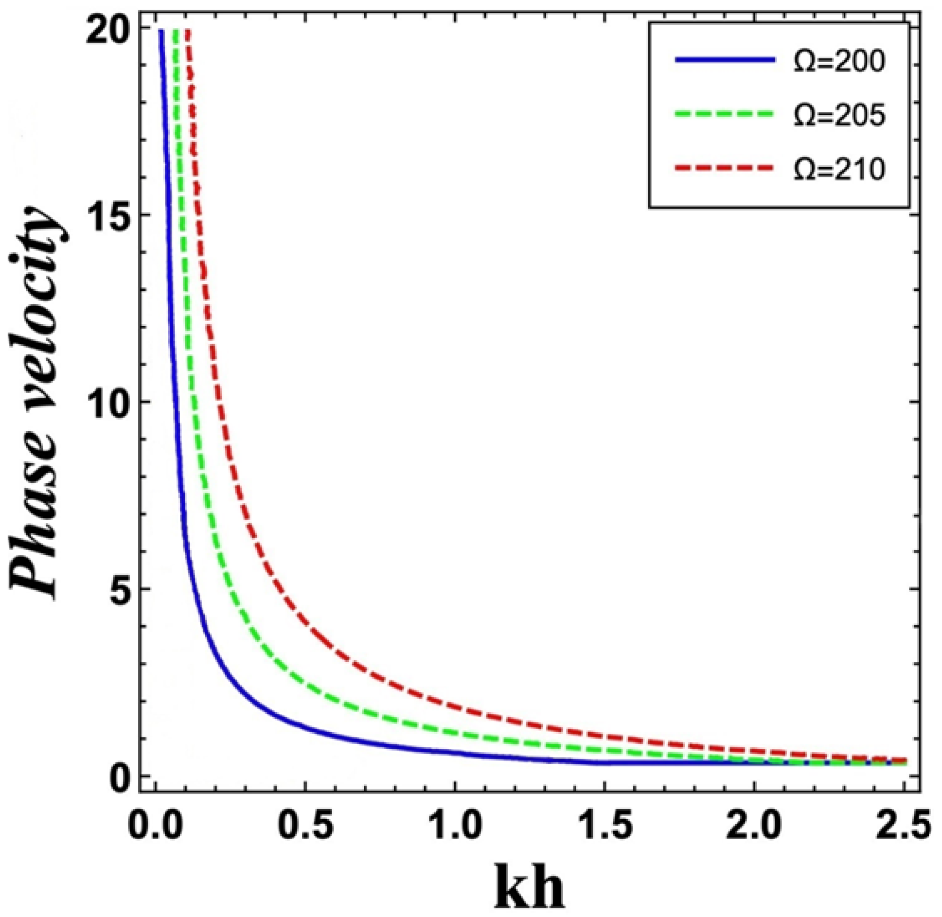
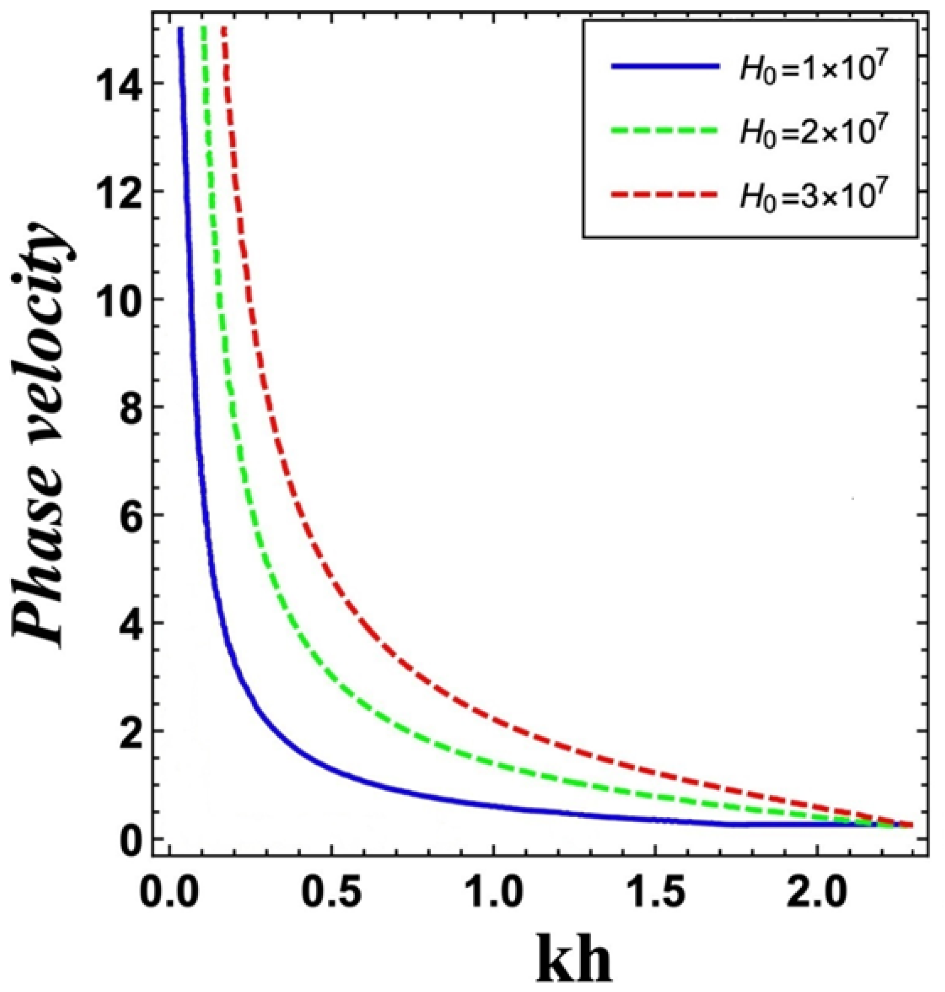
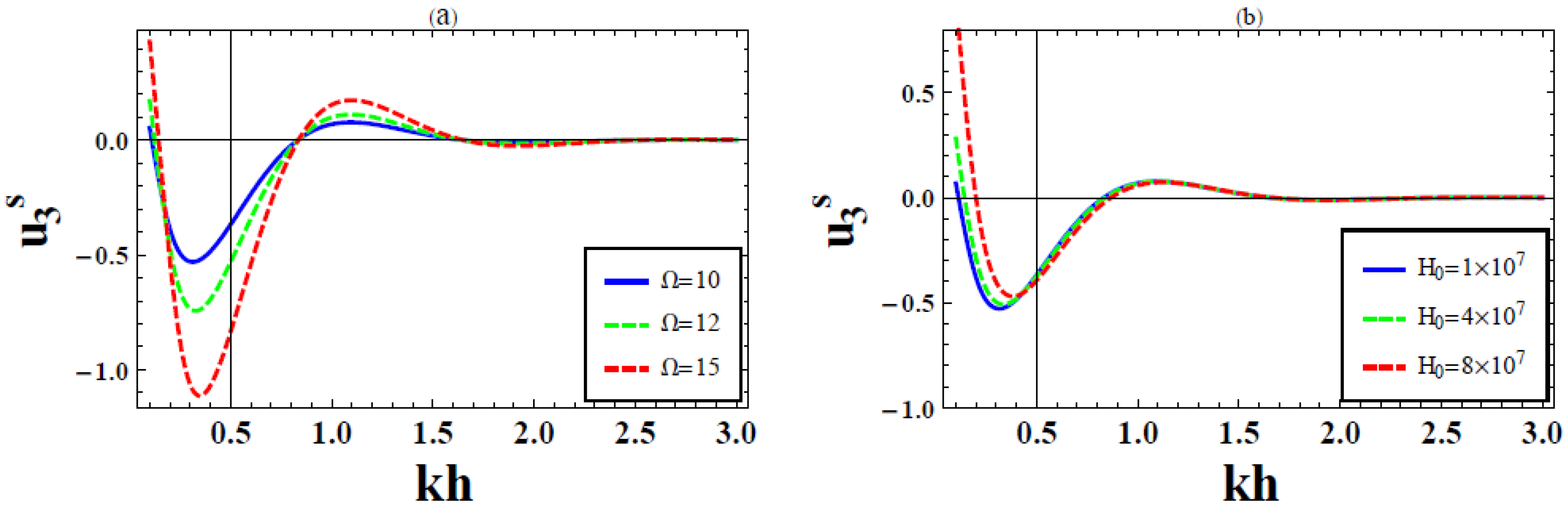
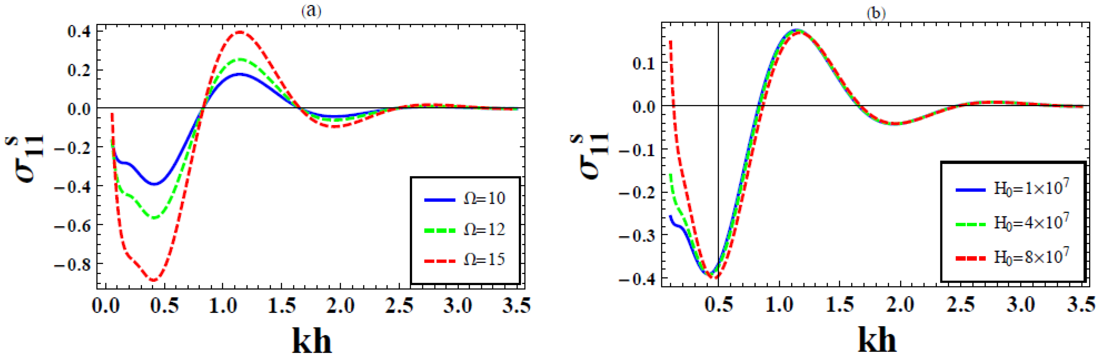
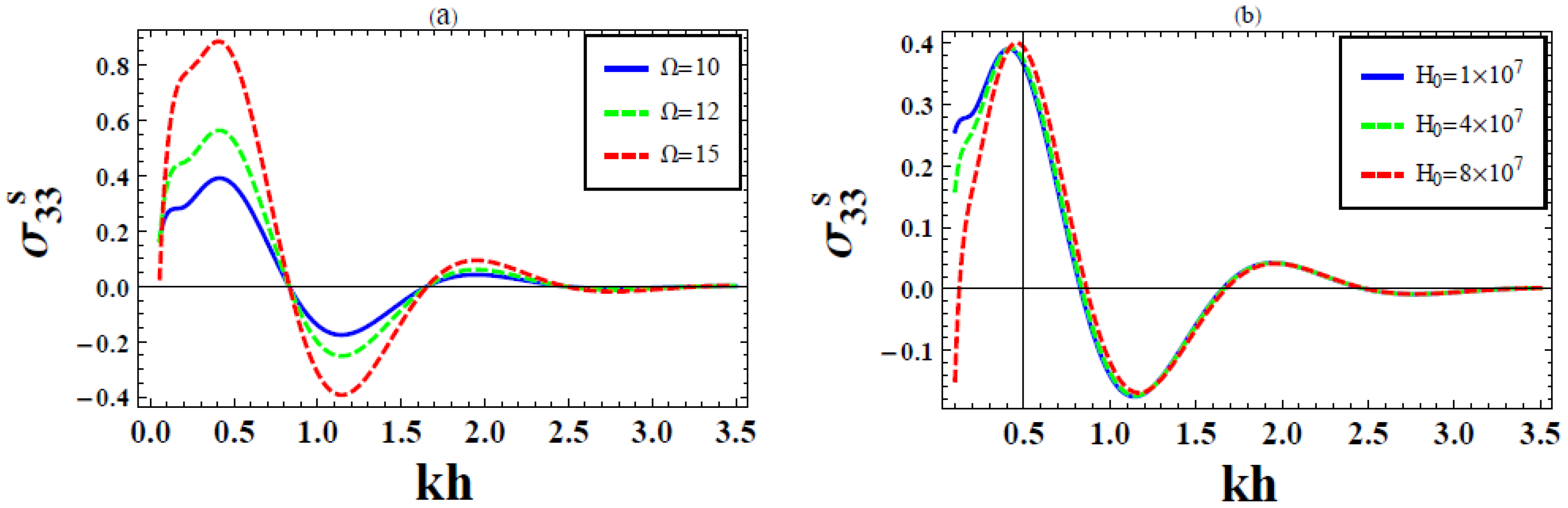
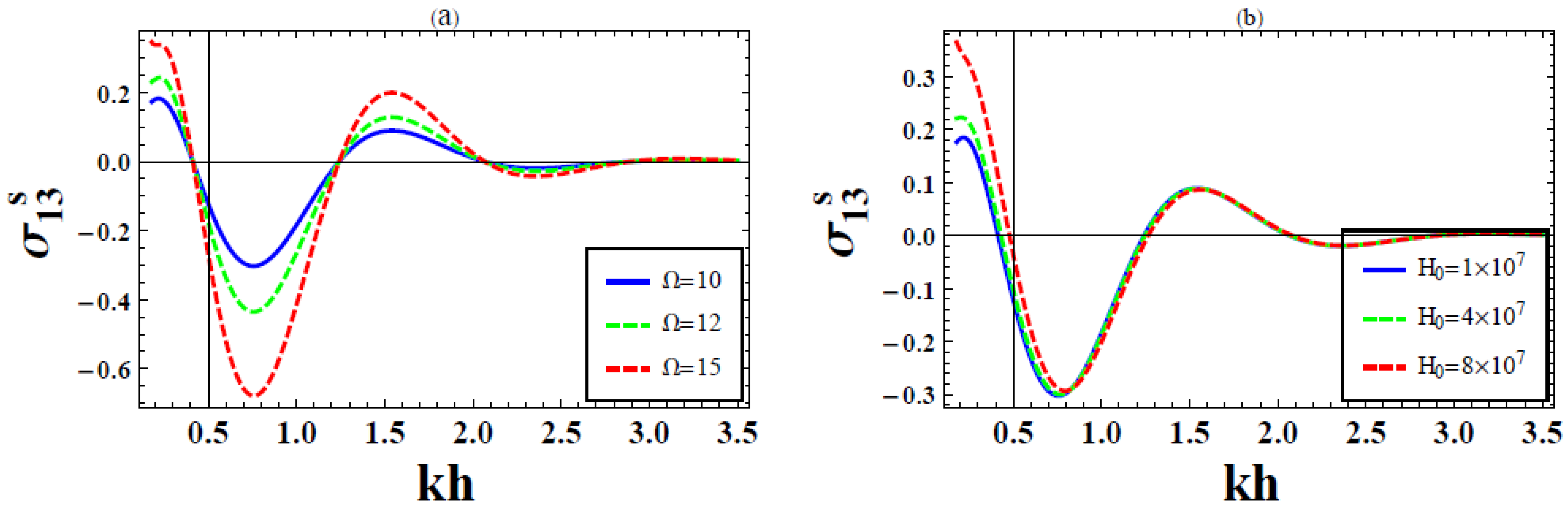
6. Numerical Results and Discussion

This section gives the numerical simulation and results of the formulated problem by considering some physical data of interest in both the coating and half-space. Moreover, copper material is considered for the coating layer, while aluminum is chosen for the half-plane, which respectively admit the following physical data [23,28,29]:
ρ c = 8.954 × 10 3 kgm 3 , λ c = 7.76 × 10 10 Nm 2 μ c = 3.86 × 10 10 Nm 2 ,
ρ s = 2.7 × 10 3 kgm 3 , λ s = λ 1 = 5.775 × 10 10 Nm 2 , μ s = μ 1 = 2.643 × 10 10 Nm 2 ,
μ 0 = 4 π × 10 7 H m 1 , ε 0 = 8.85 × 10 12 H m 1 , g = 10 N .
Next, we give the graphical depictions of the obtained frequency equation in Figure 2 and Figure 3, depicting the variation of the phase velocity against the dimensionless wave number k h with the variation of the rotation and magnetic field intensity, respectively. In addition, Figure 4a,b, Figure 5a,b, Figure 6a,b and Figure 7a,b show the depictions of the resulting displacements and stresses in the half-space, being the layer of interest against the dimensionless wave number k h with the variation of the respective rotation and magnetic field intensity. It is also worth mentioning here that the viscoelasticity index is considered to be of order unity, n = 1 .
Figure 2 and Figure 3 show the graphical illustrations of the obtained frequency equation in Equation (36) by depicting the variation of the dimensional phase velocity c against the dimensionless wave number k h with the variation of the rotation and magnetic field intensity, respectively. It is observed in both figures that the dispersion curve—more specifically, the first harmonic mode—starts off at approximately 20 ms 1 on the phase velocity axis and steadily decreases to converge at approximately 2.5 on the dimensionless wave number axis. Moreover, the dispersion increases with an increase of both the rotation and magnetic field; that is, both the rotation and magnetic field have similar effects on the propagation of the surface wave in the coated half-plane. Furthermore, Figure 4a, Figure 5a, Figure 6a, and Figure 7a analyze the variational effects of the rotation on the propagation of surface waves, while their corresponding (b)s examine the variational influence of the magnetic field effects on the propagation.
For instance, Figure 4a shows the propagation of the dimensionless transverse vibrational displacement u 3 s of the half-space layer against the dimensionless wave number k h with the variation of the rotational effect. It is noted from the figure that the transverse vibrational displacement starts off by decreasing with an increase in the angular velocity (rotation) before a subsequent periodic rise to the positive side of the displacement axis and thereafter converges steadily to zero as the wave number grows bigger. Moreover, Figure 4b shows the propagation of the dimensionless transverse vibrational displacement u 3 s of the half-space layer against the dimensionless wave number k h with the variation of the magnetic field intensity. It is clear from the plot that the displacement is enhanced by the presence of the magnetic force as the propagation progresses in accordance with the presence of the magnetic field intensity as the dimensionless wave number tends to infinity.
Figure 5a shows the propagation of the dimensionless normal stress σ 11 s of the half-space layer against the dimensionless wave number k h with the variation of the rotational effect. Here, it is noted from the figure that the normal stress starts off by decreasing with an increase in the angular velocity (rotation) before a subsequent periodic increase to the positive side of the stress axis, oscillates a little, and further steadily converges to zero as the wave number increases. In addition, from Figure 5b, the evolution of the dimensionless normal stresses σ 11 s of the half-space layer against the dimensionless wave number k h with the variation of the magnetic field intensity is portrayed. In the figure, periodic behavior is equally observed as the profile responds periodically to the presence of the magnetic field force. Moreover, one can also conclude that the influence is not that significant, looking at the variation in the bulk part of the curves; the significance is observed on the approximate range of 0 k h 0.45 , where an instant response is noted at the beginning before the subsequent smooth decline.
A similar interpretation of the above figure also applies to the corresponding normal stress σ 33 s plots portrayed in Figure 6a,b. The only difference here is that the σ 11 s begins downwardly from the negative axis of the stress and periodically progresses to the limiting point, while σ 33 s reverses the initial trend and equally tends to the limiting point. In addition, one can note from the two figures the periodic behavior being enjoyed by the stress. Moreover, one can also conclude that the presence of rotation is more significant from (a) as compared to the presence of magnetic field intensity in (b).
Furthermore, Figure 7a shows the propagation of the dimensionless shear stress σ 13 s of the half-space layer against the dimensionless wave number k h with the variation of the rotational effect. One can equally observe an oscillatory behavior of the profile that rises and falls periodically towards converging at the limit point zero. Furthermore, upon magnification, one would also deduce that the greater the increase in the angular velocity, the greater the delay in reaching the limit point. Lastly, Figure 7b portrays the periodic evolution of the dimensionless shear stress σ 13 s of the half-space layer against the dimensionless wave number k h with the variation of the magnetic field intensity. Similarly, one can equally notice an instant response on the approximate range of 0 k h 0.45 before a subsequent decline towards the limiting point as k h enlarges. To conclude, one could deduce that the presence of the rotational effect is more significant than the magnetic field, as both the displacement and stresses respond greatly to it.

7. Conclusions

In conclusion, the present manuscript examined the propagation of surface waves in a rotating coated higher-order viscoelastic half-space amidst the influence of external forces. These forces included the magnetic field and gravitational forces, in addition to the structure being assumed to be in a rotating orientation. The celebrated normal mode analysis procedure was considered as the methodology, having demonstrated a high level of efficiency in the literature. The general analytical frequency equation was determined and analyzed for certain scenarios of curiosity, in addition to the determination of the approximate analytical displacements and stresses in the rotating viscoelastic half-space. Moreover, we have considered certain physical data of relevance with viscoelasticity index of unity for the sake of the numerical simulation. To conclude, certain graphical illustrations were also depicted to portray the results of the study graphically. Hence, the presence of both the magnetic field and rotation was observed to positively accelerate the dispersion of the surface waves in the coated half-space, while sinusoidal behaviors were noted with regards to the obtained displacements and stresses. Lastly, both fields of the half-space layer were noted to respond greatly to the rotational effect, in comparison with their reaction to the presence of the magnetic field.

Author Contributions

Conceptualization, A.M., S.A. and R.I.N.; methodology, A.M. and R.I.N.; validation, A.M., S.A. and R.I.N.; formal analysis, A.M., S.A. and R.I.N.; investigation, A.M., S.A. and R.I.N.; data curation, A.M., S.A. and R.I.N.; writing—original draft preparation, R.I.N.; writing—review and editing, A.M., S.A. and R.I.N. All authors have read and agreed to the published version of the manuscript.

Funding

This research did not receive any specific external funding other than the funding by Taif University, Taif, Saudi Arabia.

Institutional Review Board Statement

Not applicable.

Informed Consent Statement

Not applicable.

Data Availability Statement

Not applicable.

Acknowledgments

Taif University Researchers Supporting Project number (TURSP-2020/305), Taif University, Taif, Saudi Arabia.

Conflicts of Interest

The authors declare no conflict of interest.

Appendix A

The coefficients of the system of ordinary differential equations given in Equations (24) and (25) are given by
l 1 = D 2 χ c 1 c c 1 2 k 2 χ c 1 c c 1 2 + Ω 2 c c 1 2 + k 2 v c 1 2 χ c 2 + k 2 v c 1 2 + D 2 k 2 ,
l 2 = i g k c c 1 2 , l 3 = i g k c c 2 2 , l 6 = i g k c s 1 2 , l 7 = i g k c s 2 2 ,
l 4 = Ω 2 c c 2 2 + k 2 v c 2 2 χ c 2 + k 2 v c 2 2 + D 2 k 2 ,
l 5 = D 2 ( i c k ) n + D 2 χ s 1 c s 1 2 k 2 ( i c k ) n k 2 χ s 1 c s 1 2 + Ω 2 c s 1 2 + k 2 v s 1 2 χ s 2 + k 2 v s 1 2 ,
l 8 = D 2 ( i c k ) n k 2 ( i c k ) n + Ω 2 c s 2 2 + k 2 v s 2 2 χ s 2 + k 2 v s 2 2 ,
where D 2 = d 2 / d x 3 2 .

Appendix B

The coefficients of the differential characteristic equations given in Equations (28) and (29) are given by
a 1 = χ c 1 c c 1 2 1 , b 1 = ( i c k ) n χ s 1 c s 1 2 ( i c k ) n ,
a 2 = c c 2 2 k 2 χ c 1 v c 2 2 χ c 2 + 1 2 + Ω 2 + Ω 2 χ c 1 c c 1 2 c c 2 2 c c 1 2 k 2 c c 2 2 v c 1 2 χ c 2 + 1 + v c 2 2 χ c 2 + 1 2 + Ω 2 c c 1 2 c c 2 2 ,
a 3 = k 2 c c 2 2 v c 2 2 χ c 2 + 1 1 k 2 χ c 1 Ω 2 + k 2 Ω 2 χ c 1 + g 2 k 2 Ω 4 c c 1 2 c c 2 2 k 2 c c 1 2 v c 1 2 χ c 2 + 1 1 k 2 c c 2 2 v c 2 2 χ c 2 + 1 1 + Ω 2 c c 1 2 c c 2 2 ,
b 2 = χ s 1 k 2 c s 2 2 v s 2 2 χ s 2 + 1 + Ω 2 + c s 2 2 ( i c k ) n Ω 2 2 k 2 χ s 1 c s 1 2 c s 2 2 + c s 1 2 ( i c k ) n Ω 2 + k 2 c s 2 2 χ s 2 + 1 v s 1 2 + v s 2 2 + 2 ( i c k ) n c s 1 2 c s 2 2 ,
b 3 = k 2 c s 2 2 k 2 χ s 1 Ω 2 v s 2 2 χ s 2 + 1 + ( i c k ) n g 2 k 2 k 2 Ω 2 χ s 1 + Ω 4 c s 1 2 c s 2 2 k 2 c s 1 2 v s 1 2 χ s 2 + 1 + ( i c k ) n Ω 2 + k 2 c s 2 2 v s 2 2 χ s 2 + 1 + ( i c k ) n c s 1 2 c s 2 2 .

Appendix C

The entries for the dispersion matrix a i j given in Equation (35) that result in the aiming frequency equation are found to be
a 11 = e α 1 h α 1 2 ξ 1 + k 2 ξ 1 + 2 i α 1 k , a 12 = e α 2 h α 2 2 ξ 2 + k 2 ξ 2 + 2 i α 2 k , a 15 = 0 , a 13 = e α 3 h α 3 2 ξ 3 + k 2 ξ 3 + 2 i α 3 k , a 14 = e α 4 h α 4 2 ξ 4 + k 2 ξ 4 + 2 i α 4 k , a 16 = 0 ,
a 21 = e α 1 h α 1 c c 1 2 α 1 i k ξ 1 + χ c 1 α 1 2 k 2 k χ c 3 k i α 1 ξ 1 , a 22 = e α 2 h α 2 c c 1 2 α 2 i k ξ 2 + χ c 1 α 2 2 k 2 k χ c 3 k i α 2 ξ 2 ,
a 23 = e α 3 h α 3 c c 1 2 α 3 i k ξ 3 + χ c 1 α 3 2 k 2 k χ c 3 k i α 3 ξ 3 , a 25 = 0 , a 24 = e α 4 h α 4 c c 1 2 α 4 i k ξ 4 + χ c 1 α 4 2 k 2 k χ c 3 k i α 4 ξ 4 , a 26 = 0 ,
a 31 = α 1 ξ 1 + i k , a 32 = α 2 ξ 2 + i k , a 33 = α 3 ξ 3 + i k , a 34 = α 4 ξ 4 + i k , a 35 = β 1 η 1 i k , a 36 = β 2 η 2 i k ,
a 41 = α 1 i k ξ 1 , a 42 = α 2 i k ξ 2 , a 43 = α 3 i k ξ 3 , a 44 = α 4 i k , ξ 4 , a 45 = β 1 + i η 1 k , a 46 = β 2 + i η 2 k ,
a 51 = μ c α 1 2 ξ 1 + k 2 ξ 1 + 2 i α 1 k , a 52 = μ c α 2 2 ξ 2 + k 2 ξ 2 + 2 i α 2 k , a 53 = μ c α 3 2 ξ 3 + k 2 ξ 3 + 2 i α 3 k , a 54 = μ c α 4 2 ξ 4 + k 2 ξ 4 + 2 i α 4 k ,
a 55 = μ 1 ( i c k ) n β 1 2 η 1 + η 1 k 2 + 2 i β 1 k , a 56 = μ 1 ( i c k ) n β 2 2 η 2 + η 2 k 2 + 2 i β 2 k ,
a 61 = ρ c α 1 c c 1 2 α 1 i k ξ 1 + χ c 1 α 1 2 k 2 k χ c 3 k i α 1 ξ 1 , a 62 = ρ c α 2 c c 1 2 α 2 i k ξ 2 + χ c 1 α 2 2 k 2 k χ c 3 k i α 2 ξ 2 , a 63 = ρ c α 3 c c 1 2 α 3 i k ξ 3 + χ c 1 α 3 2 k 2 k χ c 3 k i α 3 ξ 3 , a 64 = ρ c α 4 c c 1 2 α 4 i k ξ 4 + χ c 1 α 4 2 k 2 k χ c 3 k i α 4 ξ 4 ,
a 65 = ρ s β 1 c s 1 2 ( i c k ) n β 1 i η 1 k k χ s 3 ( i c k ) n k i β 1 η 1 + β 1 2 k 2 χ s 1 , a 66 = ρ s β 2 c s 1 2 ( i c k ) n β 2 i η 2 k k χ s 3 ( i c k ) n k i β 2 η 2 + β 2 2 k 2 χ s 1 .

Appendix D

The entries for the respective reduced frequency equations b i j and c i j given in Equations (37) and (39) are determined to be
b 11 = β 1 2 η 1 + η 1 k 2 + 2 i β 1 k , b 12 = β 2 2 η 2 + η 2 k 2 + 2 i β 2 k ,
b 21 = β 1 c s 1 2 ( i c k ) n β 1 i η 1 k k χ s 3 ( i c k ) n k i β 1 η 1 + β 1 2 k 2 χ s 1 , b 22 = β 2 c s 1 2 ( i c k ) n β 2 i η 2 k k χ s 3 ( i c k ) n k i β 2 η 2 + β 2 2 k 2 χ s 1 ,
c 11 = k i β 1 η 1 , c 12 = k i β 2 η 2 , c 21 = β 1 i η 1 k , c 22 = β 2 i η 2 k .

References

  1. Achenbach, J. Wave Propagation in Elastic Solids; Elsevier: Amsterdam, The Netherlands, 2012. [Google Scholar]
  2. Brigatti, M.F.; Mottana, A. Layered Mineral Structures and Their Application in Advanced Technologies; The Mineralogical Society of Great Britain and Ireland: Twickenham, UK, 2011; Volume 11. [Google Scholar] [CrossRef]
  3. Ewing, W.M.; Jardetzky, W.S.; Press, F.; Beiser, A. Elastic Waves in Layered Media. Phy. Today 1957, 10, 27. [Google Scholar] [CrossRef]
  4. Kaplunov, J.D.; Kossovitch, L.Y.; Nolde, E.V. Dynamics of Thin Walled Elastic Bodies; Academic Press: Cambridge, MA, USA, 1998. [Google Scholar]
  5. Nuruddeen, R.I.; Nawaz, R.; Zia, Q.M.Z. Asymptotic approach to anti-plane dynamic problem of asymmetric three-layered composite plate. Math. Methods Appl. Sci. 2021, 44, 10933–10947. [Google Scholar] [CrossRef]
  6. Nuruddeen, R.I.; Nawaz, R.; Zia, Q.M.Z. Investigating the viscous damping effects on the propagation of Rayleigh waves in a three-layered inhomogeneous plate. Phy. Scr. 2020, 95, 065224. [Google Scholar] [CrossRef]
  7. Bose, S. High Temperature Coatings; Elsevier: Amsterdam, The Netherlands, 2017. [Google Scholar]
  8. Chattopadhyay, D.K.; Raju, K.V.S.N. Structural engineering of polyurethane coatings for high performance applications. Prog. Polym. Sci. 2007, 32, 352–418. [Google Scholar] [CrossRef]
  9. Datta, P.K. Surface Engineering: Engineering Applications; Royal Society of Chemistry: London, UK, 1993. [Google Scholar]
  10. Padture, N.P.; Gell, M.; Jordan, E.H. Thermal barrier coatings for gas-turbine engine applications. Science 2002, 296, 280–284. [Google Scholar] [CrossRef] [PubMed]
  11. Dai, H.-H.; Kaplunov, J.; Prikachikov, D.A. A long-wave model for the surface wave in a coated half-space. Proc. R. Soc. A Math. Phy. Eng. Sci. 2010, 466, 3097–3116. [Google Scholar] [CrossRef] [Green Version]
  12. Li, M.; Liu, Q.; Jia, Z.; Xu, X.; Cheng, Y.; Zheng, Y.; Xi, T.; Wei, S. Graphene oxide/hydroxyapatite composite coatings fabricated by electrophoretic nanotechnology for biological applications. Carbon 2014, 67, 185–197. [Google Scholar] [CrossRef]
  13. Tiainen, V.M. Amorphous carbon as a bio-mechanical coating-mechanical properties and biological applications. Diamond Rel. Mat. 2001, 10, 153–160. [Google Scholar] [CrossRef]
  14. Qian, Z.; Jin, F.; Kishimoto, K.; Wang, Z. Effect of initial stress on the propagationn behavior of SH-waves in multilayered piezoelectric composite structures. Sens. Actuators A Phys. 2004, 112, 368–375. [Google Scholar] [CrossRef]
  15. Biot, M.A. Thermoelasticity and irreversible thermodynamics. J. Appl. Phy. 1956, 27, 240–253. [Google Scholar] [CrossRef]
  16. Lord, H.W.; Shulman, Y. A generalized dynamical theory of thermoelasticity. J. Mech. Phy. Solids. 1967, 15, 299–309. [Google Scholar] [CrossRef]
  17. Green, A.E.; Lindsay, K.A. Thermoelasticity. J. Elast. 1972, 2, 1–7. [Google Scholar] [CrossRef]
  18. Green, A.E.; Naghdi, P.M. Thermoelasticity without energy dissipation. J. Elast. 1993, 31, 189–208. [Google Scholar] [CrossRef]
  19. Chandrasekharaih, D.S. Thermoelasticity with second sound: A review. Appl. Mech. Rev. 1986, 39, 355–376. [Google Scholar] [CrossRef]
  20. Chandrasekharaih, D.S. Hyperbolic thermoelasticity: A review of recent literature. Appl. Mech. Rev. 1998, 51, 705–729. [Google Scholar] [CrossRef]
  21. Yu, J.; Ma, Q.; Su, S. Wave propagation in non-homogeneous magneto-electro-elastic hollow cylinders. Ultras 2008, 48, 664–677. [Google Scholar] [CrossRef] [PubMed]
  22. Ebrahimi, F.; Barati, M.R.; Dabbagh, A. Wave propagation in embedded inhomogeneous nanoscale plates incorporating thermal effects. Waves Random Complex Media 2018, 28, 215–235. [Google Scholar] [CrossRef]
  23. Abo-Dahab, S.M.; Lotfy, K.; Gohaly, K.A. Rotation and magnetic field effect on surface waves propagation in an elastic layer lying over a generalized thermoelastic diffusive half-space with imperfect boundary. Math. Probl. Eng. 2015, 2015, 671783. [Google Scholar] [CrossRef] [Green Version]
  24. Wang, Y.Z.; Li, F.M.; Kishimoto, K. Thermal effects on vibration properties of double-layered nanoplates at small scales. Compos. Part B Eng. 2011, 42, 1311–1317. [Google Scholar] [CrossRef]
  25. Selim, M.M. Effect of thermal stress and magnetic field on propagation of transverse wave in an anisotropic incompressible dissipative initially stressed plate. Appl. Math. Inf. Sci. 2017, 11, 195–200. [Google Scholar] [CrossRef]
  26. Erbaş, B.; Kaplunov, J.; Nobili, A.; Kılıç, G. Dispersion of elastic waves in a layer interacting with a Winkler foundation. J. Acoust Soc. Am. 2018, 144, 2918–2925. [Google Scholar] [CrossRef] [Green Version]
  27. Abd-Alla, A.M.; Abo-Dahab, S.M.; Khan, A. Rotational effects on magneto-thermoelastic Stoneley, Love, and Rayleigh waves in fibre-reinforced anisotropic general viscoelastic media of higher order. Comp. Mat. Continua. 2017, 53, 49–72. [Google Scholar]
  28. Farhan, A.M.; Abd-Alla, A.M. Effect of rotation on the surface wave propagation in magneto-thermoelastic materials with voids. J. Ocean Engr. Sci. 2018, 3, 334–342. [Google Scholar] [CrossRef]
  29. Nuruddeen, R.I.; Nawaz, R.; Zia, Q.M.Z. Dispersion of elastic waves in an asymmetric three-layered structure in the presence of magnetic and rotational effects. Prog. Electr. R. 2020, 91, 165–177. [Google Scholar] [CrossRef]
  30. Abbas, I.A. Eigenvalue approach in a three-dimensional generalized thermoelastic interactions with temperature-dependent material properties. Comp. Math. Appl. 2014, 68, 2036–2056. [Google Scholar] [CrossRef]
  31. Zennir, K.; Allahem, A.; Cherif, B. Quantitative studies for a magneto-visco-elastic system and its applications. Int. J. Appl. Math. Stat. 2018, 57, 1–15. [Google Scholar]
  32. Nuruddeen, R.I.; Nawaz, R.; Zia, Z.Q.M. Effects of thermal stress, magnetic field and rotation on the dispersion of elastic waves in an inhomogeneous five-layered plate with alternating components. Sci. Prog. 2020, 103, 0036850420940469. [Google Scholar] [CrossRef]
  33. Zennir, K.; Allahem, A.; Boulaaras, S.; Cherif, B. New mathematical studies for surface waves on multi-layered liquid films. Int. J. Eng. Res. Tech. 2019, 12, 269–275. [Google Scholar] [CrossRef]
  34. Gholami, A.; Ganji, D.D.; Rezazadeh, H.; Adel, W.; Bekir, A. Application of modified Mickens iteration procedure to a pendulum and the motion of a mass attached to a stretched elastic wire. Int. J. Nonlinear Sci. Num. Simul. 2021. [Google Scholar] [CrossRef]
  35. Al-Duhaim, H.R.; Yilbas, B.S.; Zaman, F.D. Determination of temperature distribution and thermal stress for the hyperbolic heat conduction equation due to laser short pulse heating. Lasers Eng. 2016, 35, 275–301. [Google Scholar]
  36. Nawaz, R.; Nuruddeen, R.I.; Zia, Q.M.Z. An asymptotic investigation of the dynamics and dispersion of an elastic five-layered plate for anti-plane shear vibration. J. Eng. Math. 2021, 128, 1–12. [Google Scholar] [CrossRef]
  37. Davodi, A.G.; Rezazadeh, H.; Adel, W.; Bekir, A.; Ganji, D.D. Fluctuation and frequency of the oscillators with exponential spring using accurate approximate analytical solutions. Fluct. Noise Lett. 2021, 20, 2150036. [Google Scholar] [CrossRef]
  38. Miyasita, T.; Zennir, K. Finite time blow-up for a viscoelastic wave equation with weak-strong damping and power nonlinearity. Osaka J. Math. 2021, 58, 661–669. [Google Scholar]
  39. Dridi, H.; Zennir, K. New class of Kirchhoff type equations with Kelvin-Voigt damping and general nonlinearity: Local existence and blow-up in solutions. J. Partial. Diff. Equ. 2021, 34, 313–347. [Google Scholar]
  40. Biot, M.A. Mechanics of Incremental Deformations; Wiley: New York, NY, USA, 1965. [Google Scholar]
  41. Ting, T.C.T. Surface waves in an exponentially graded, general anisotropic elastic material under the influence of gravity. Wave Motion 2011, 48, 335–344. [Google Scholar]
  42. Mubaraki, A.M.A. Asymptotic Models for Surface Waves in Coated Elastic Solids. Ph.D. Thesis, Keel University, Keele, UK, 2021. [Google Scholar]
  43. Abo-Dahab, S.M.; Abd-Alla, A.M.; Khan, A. Rotational effect on Rayleigh, Love and Stoneley waves in non-homogeneous fibre-reinforced anisotropic general viscoelastic media of higher order. Struc. Eng. Mech. 2016, 58, 181–197. [Google Scholar] [CrossRef]
  44. Younesian, D.; Hosseinkhani, A.; Askari, H.; Esmailzadeh, E. Elastic and viscoelastic foundations: A review on linear and nonlinear vibration modeling and applications. Nonlinear Dyn. 2019, 97, 1–43. [Google Scholar] [CrossRef]
Figure 1. A coated elastic half-space under external forces.
Fractalfract 05 00250 g001
Figure 2. Response of the dimensional dispersion relation to the variation of the dimensional rotation.
Fractalfract 05 00250 g002
Figure 3. Response of the dimensional dispersion relation to the variation of the dimensional magnetic field intensity.
Fractalfract 05 00250 g003
Figure 4. Variation of the dimensionless displacement u 3 s versus dimensionless wave number with respect to the dimensional (a) rotation and (b) magnetic field intensity.
Fractalfract 05 00250 g004
Figure 5. Variation of the dimensionless normal stress σ 11 s versus dimensionless wave number with respect the dimensional (a) rotation and (b) magnetic field intensity.
Fractalfract 05 00250 g005
Figure 6. Variation of the dimensionless normal stress σ 33 s versus dimensionless wave number with the dimensional (a) rotation and (b) magnetic field intensity.
Fractalfract 05 00250 g006
Figure 7. Variation of the dimensionless shear stress σ 13 s versus dimensionless wave number with respect the dimensional (a) rotation and (b) magnetic field intensity.
Fractalfract 05 00250 g007
Publisher’s Note: MDPI stays neutral with regard to jurisdictional claims in published maps and institutional affiliations.

