
Fractals as Julia Sets of Complex Sine Function via Fixed Point Iterations


1
BGR Campus, Hemavati Nandan Bahuguna Garhwal University, Pauri Garhwal 246001, India
2
Pt. L.M.S. Campus, Sri Dev Suman Uttrakhand University, Rishikesh 249201, India
3
M.B. Patel Institute of Technology, New Vallabh Vidyanagar 388121, India
4
Department of Mechanical Engineering, College of Engineering, Qassim University, Buraydah 51452, Saudi Arabia
*
Author to whom correspondence should be addressed.
Fractal Fract. 2021, 5(4), 272; https://0-doi-org.brum.beds.ac.uk/10.3390/fractalfract5040272
Submission received: 13 November 2021
/
Revised: 8 December 2021
/
Accepted: 9 December 2021
/
Published: 14 December 2021
(This article belongs to the Special Issue Convergence and Dynamics of Iterative Methods: Chaos and Fractals)
Abstract
:We explore some new variants of the Julia set by developing the escape criteria for a function , where , , and z is a complex variable, utilizing four distinct fixed point iterative methods. Furthermore, we examine the impact of parameters on the deviation of dynamics, color, and appearance of fractals. Some of these fractals represent the stunning art on glass, and Rangoli (made in different parts of India, especially during the festive season) which are useful in interior decoration. Some fractals are similar to beautiful objects found in our surroundings like flowers (to be specific Hibiscus and Catharanthus Roseus), and ants.
MSC:
28A10; 31E05; 37F10; 37F46; 47H101. Introduction
Due to the self-similarity, the study of fractals emerged as the most fascinating area of research [1,2]. The investigation on fractals commenced at the beginning of the twentieth century, when French mathematician Gaston Maurice Julia and French mathematician and astronomer Pierre Joseph Louis Fatou studied complex dynamics and determined the successive approximations of the complex function , c is a complex number and z is a complex variable. In 1918, Julia [3,4] was successful at iterating this function but could not sketch it. Fatou [5] was the first to study the Julia sets. This is why its complement is often known as the Fatou set. It comprises values possessing the characteristic that all neighboring values act in the same way under repeated iteration of the underlying function. On the other hand, the Julia set comprises values having the property that even an arbitrarily small perturbation may create serious changes in the sequence of iterated functions. Consequently, the function on the Fatou set behaves in a “regular” manner, on the other hand, the function on the Julia set behaves in a “chaotic” manner. Later on, around 1980, a Polish-born French-American mathematician and polymath Benoit B. Mandelbrot [1] drew the Julia set and investigated its characteristics. He gave the name fractals to these complex graphs and noticed that, for distinct values of the parameter c, the Julia sets possess distinctiveness in their characteristics. In addition, on interchanging the position of z and c, he introduced a new set widely known as the Mandelbrot set in which we investigate the connectedness of the Julia set for every value of c. On the contrary, in the Julia set, we investigate the behavior of the iterates for every value of z. In 1987, Lakhtakia et al. [6] extended their work by utilizing , and, in 1989, Crowe et al. [7] sketched complex graphs for and introduced the anti-Julia and anti-Mandelbrot sets to discuss their connected locus. These graphs are termed as “tricorn” [8]. Since then, numerous generalizations of fractals have come into the existence via different fixed point iterative methods (for instance, Mann-iteration [9], Ishikawa-iteration [10], S-iteration [11], Noor-iteration [12], Jungck-type iterations [13,14,15,16,17,18,19], -iteration [20], -iteration [21], and so on). Fractals for transcendental complex functions were studied in [22,23,24,25,26,27,28]. It is interesting to mention here that an iteration method, also known as a method of successive approximations, permits finding a solution with a predetermined accuracy and may be easily programmed. Consequently, it is convenient to use in computer calculations. In addition, this reduces the time of calculation and is self-correcting because the small errors that are committed in the calculation process of successive approximations may be corrected later. Iteration methods have many real-life applications. For instance, the Hybrid–Euler method [29] which is a blend of Euler’s method [30] and the spline interpolation method (suitable for smooth functions which do not have oscillating behavior [31]) has been utilized to predict the total number of infected people and the number of active cases for COVID-19 propagation to describe the dynamics of the pandemic.
In the current work, we explore some novel variants of the Julia set for the transcendental complex function of the type , a and c are complex numbers, and z is a complex variable via utilizing four distinct celebrated fixed point iterative methods. First, we develop the escape criteria in algorithms for this transcendental complex sine function, and then we utilize it to sketch Julia sets. It is worth mentioning here that the algorithms perform a significant role in sketching the fractals while, the escape limitations are fundamental requirements for running the algorithms. Finally, we compare the sketched complex graphics in Picard-orbit, Mann-orbit, Ishikawa-orbit, and Noor-orbit and examine the response of stunning Julia sets for distinct variables via these distinct algorithms.
2. Preliminaries
The filled Julia set [2,3] of the polynomial over the set of complex numbers of degree is defined as
Noticeably, it is a set of complex numbers for which the orbits do not converge to a point at infinity. The Julia set of p is the boundary of , that is,
Definition 1.
Let be a complex valued self-map. For , and ,
- (i)
- the Picard-iteration [32] isClearly, it is a one-step feedback procedure.
- (ii)
- the Mann-iteration [9] isClearly, it is a one-step feedback procedure.
- (iii)
- the Ishikawa-iteration [10] isClearly, it is a two-step feedback procedure.
- (iv)
- the Noor-iteration [12] isClearly, it is a three-step feedback procedure.
Remark 1.
The Noor-orbit diminishes to:
- 1.
- Ishikawa-orbit when ,
- 2.
- Mann-orbit when .
- 3.
- Picard-orbit when
Motivated by the applications of the function sine, for instance, in modeling periodic phenomena like the velocity and position of harmonic oscillators, light and sound waves, day length and sunlight intensity, average temperature variations throughout the year, and so on, we utilize sine function to explore some fascinating fractals via four different fixed point iterations. The sine function can be traced to the jyā functions utilized by Indian mathematicians and Astronomers (Aryabhatiya, Surya Siddhanta). However, jyā is a function of arcs of circles instead of angles. The modern trigonometric function of sine is a function of an angle whose only real fixed point is zero. The more improved version expresses the sine as an infinite series, allowing their extension to arbitrary negative, positive, and complex numbers.
It is well known that , and
and
We take as and and assume that
- (i)
- ,
- (ii)
- ,
- (iii)
where except the values of for which
3. Escape Criteria for Complex Sine Functions
By utilizing four distinct celebrated iterations, we prove here an escape criterion for the transcendental complex sine function of the type , a, , .
Theorem 1.
Let , , , . If the sequence is Picard-iteration, then as .
Proof.
Let . If ,
Because , where except the values of z for which , . Thus, we get
For , we have
Because and , this implies that
On iterating till kth term,
Since , where , this yields . Therefore, the orbit of z tends to infinity, that is, when . □
Theorem 2.
Let , , , . If the sequence is Mann-iteration, then as .
Proof.
Let , and
If ,
Because , where except the values of z for which , . Thus, we get
If , we have
Since and , this implies that
On iterating until the kth term,
Since , where , this yields . Therefore, the orbit of z tends to infinity, that is, when . □
Corollary 1.
Let . Since , , then when .
Theorem 3.
Let , , , and . If the sequence is Ishikawa-iteration, then as .
Proof.
Let , and
If ,
Since , where except the values of z for which , . Thus, we get
Since , this provides that .
Now, for the next step of Ishikawa-iteration, we have
Again if ,
Since , where except the values of z for which , . In addition, . Thus, we get
Now, on iterating up to kth term, we obtain
Since and , , this implies that
Hence, and the orbit of z tends to infinity, that is, when . □
Corollary 2.
Let . Since , therefore, . Hence, when .
Theorem 4.
Let , , , , and . If the sequence is Noor-iteration, then as .
Proof.
Let , and
If ,
Since , where , except the values of z for which , . Thus, we get
Since , this gives that .
Now, for the next step of Noor-iteration, we have
If ,
Since , where except the values of z for which , . In addition, . Thus, we get
Since , this provides that .
Now, for the next step of Noor-iteration, we have
Again if ,
Since , where except the values of z for which , . In addition, . Thus, we get
Now, on iterating up to kth term, we obtain
Since , and , where that is,
Therefore,
and the orbit of z tends to infinity that is, when . □
Corollary 3.
Let . Since , so . Then, as .
Remark 2.
- (i)
- The selection of the parameters in the above theorems is new and has not been studied till now in this perspective.
- (ii)
- The Corollaries 1, 2 and 3 provide algorithms for exploring Julia sets of . If , we obtain the orbit of z. If lies in the exterior of the circle of radius for some k, then the orbit escapes meaning, thereby z is not inside the Julia sets. However, if does not exceed this bound, then utilizing the definitions of the Julia sets, we utilize these algorithms to generate fractals in the next section.
4. Generation of Julia Sets
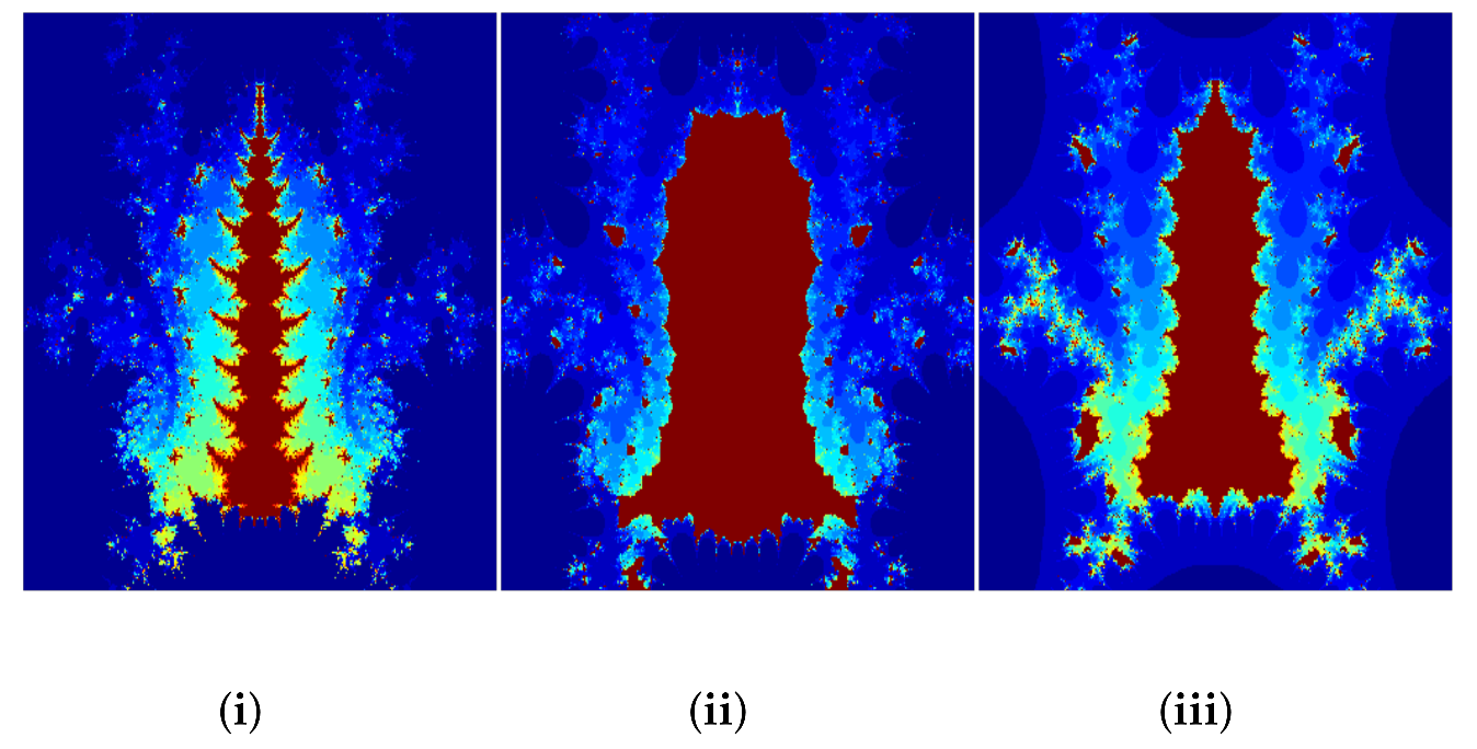
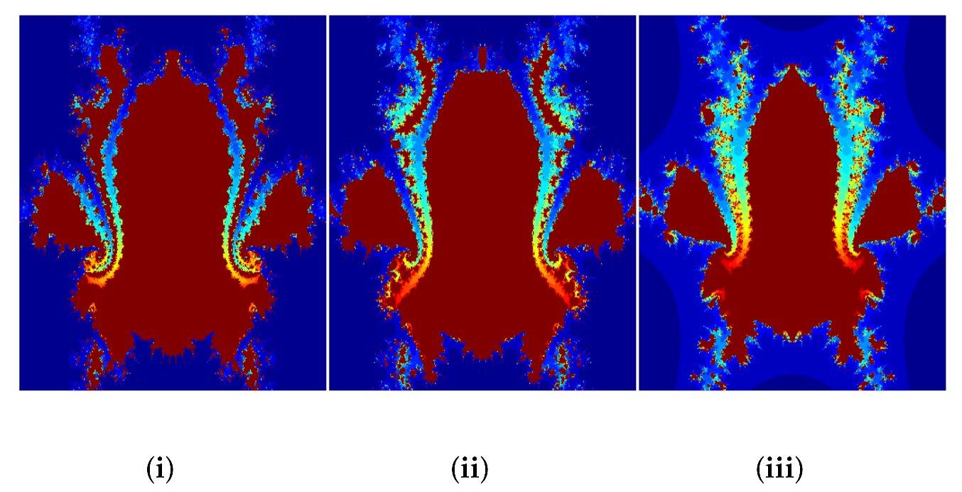
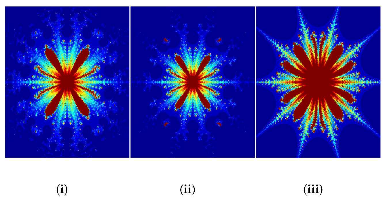
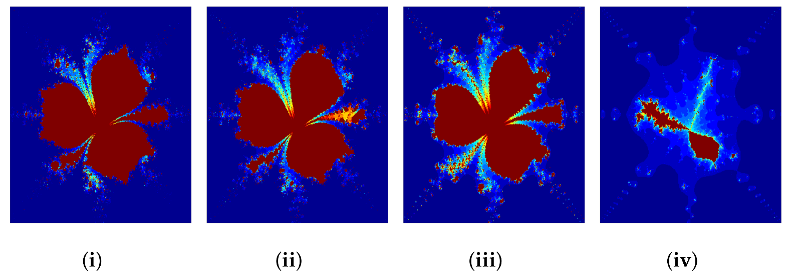
We attempt to obtain the non-classical Julia sets in four distinct orbits using Matlab 8.5.0 (R20015a). It has been observed from Figure 1 that the corresponding Julia sets for almost all the methods have no significant difference except in the Picard-iteration. However, as the iteration changes from one step to three steps, more beautiful results are noticed. We notice that, for Picard-iteration, we get a Julia set only in the neighborhood of 0. Moreover, the small change in any of the parameters gives the major change in the output. Therefore, we fix almost all the parameters and obtain the results for distinct iteration methods which are visible in the figures given below.
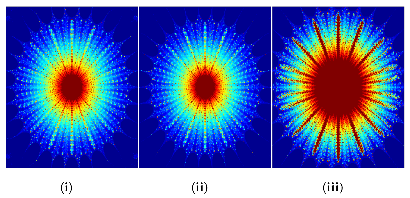
In Figure 8(i), (ii) fractals are looking like ants and in Figure 8(iii), Figure 9, Figure 10 and Figure 11, fractals are looking like Rangoli. As n increases the fractal takes a circular shape (see Figure 11 of the higher-order (n = 15) Julia set which looks like a colorful teething ring or circular saw or may be compared to glass paintings.
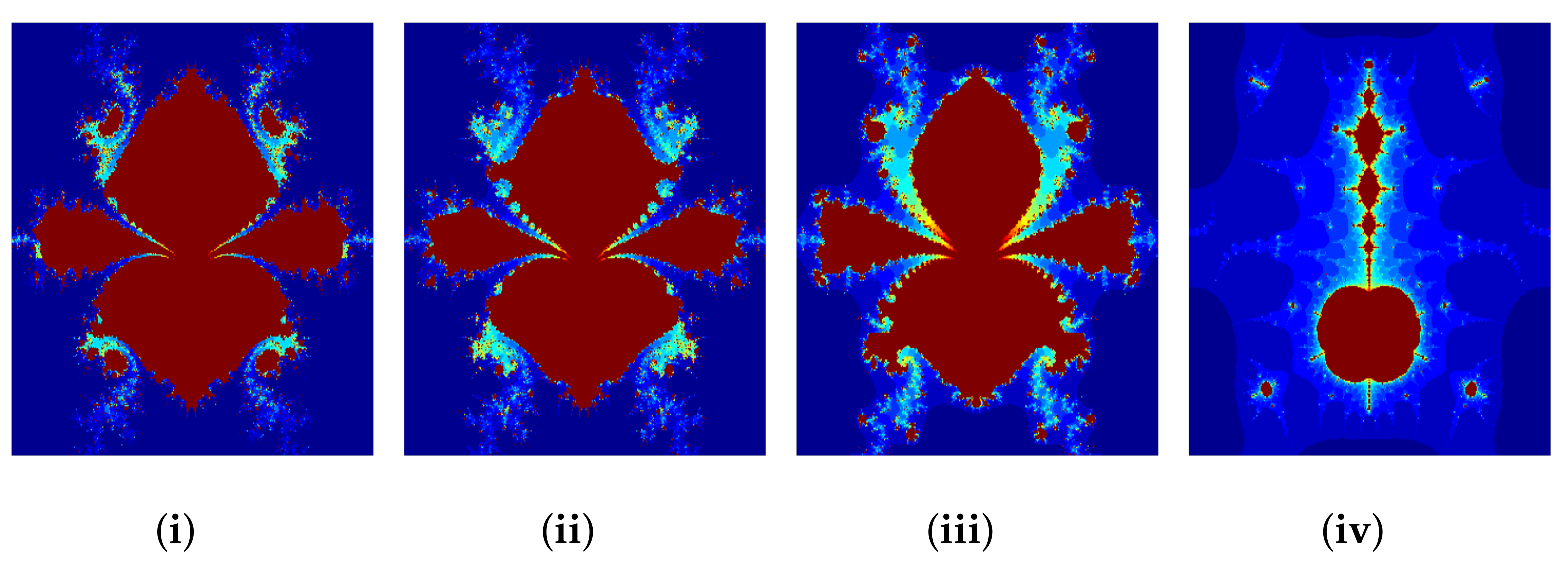
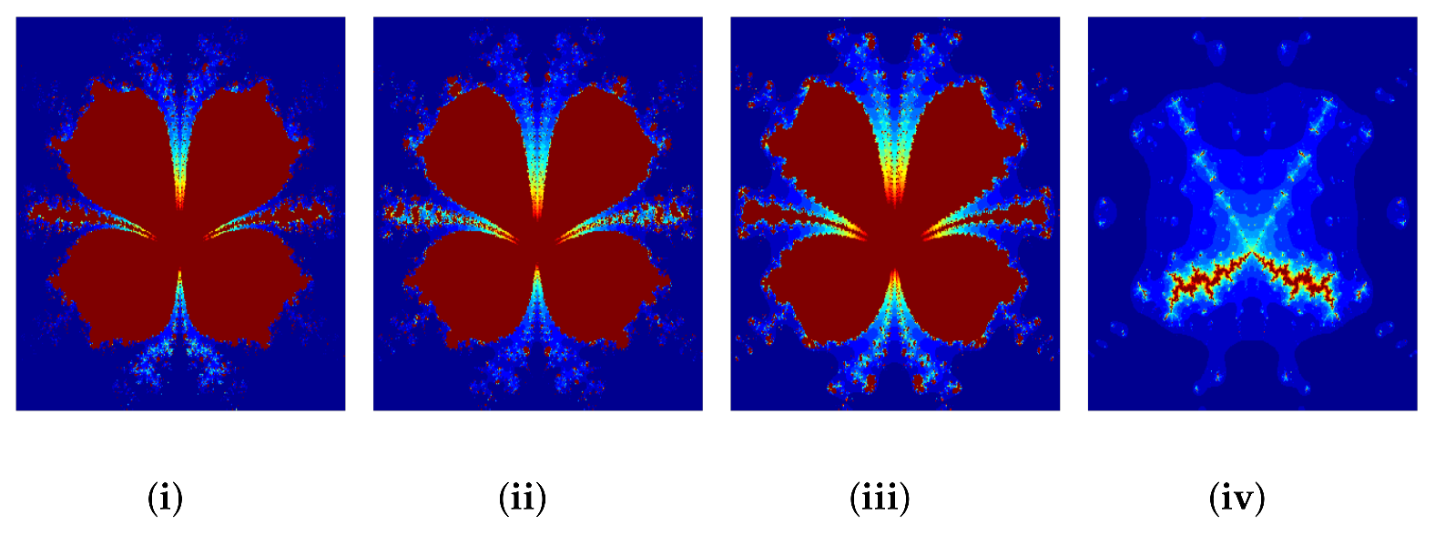
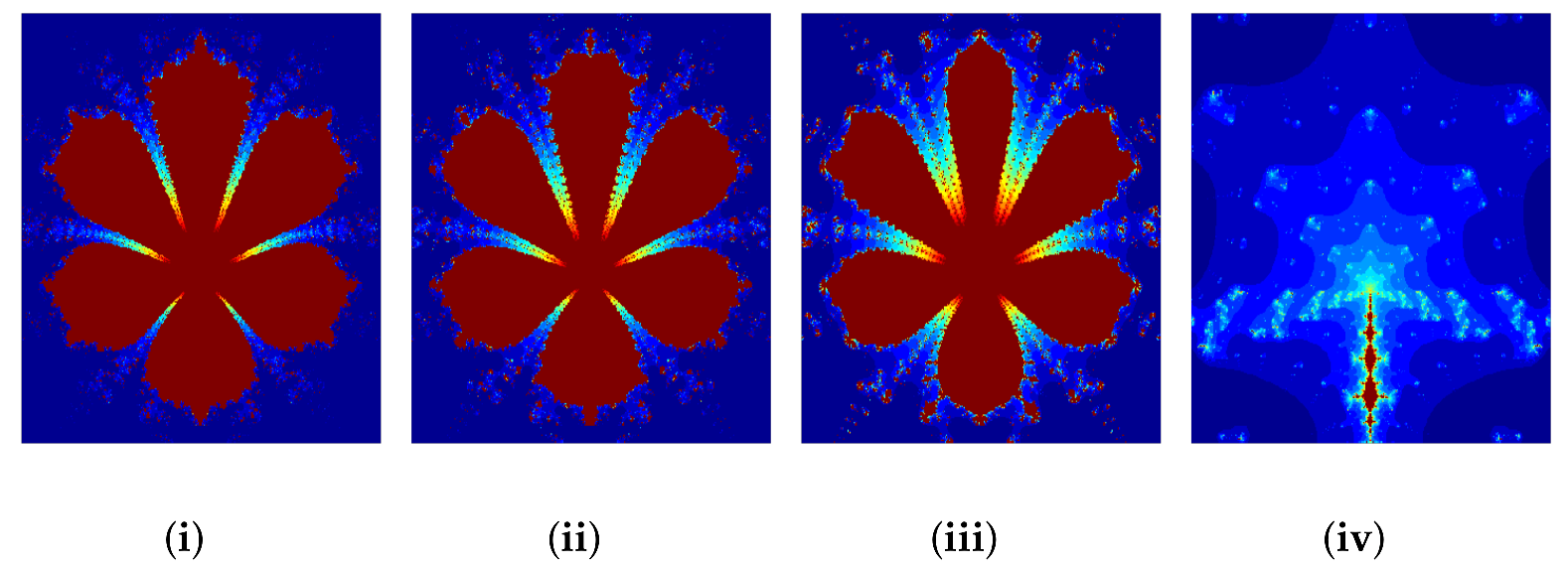
With the above parameters, we did not get Julia sets in Picard-orbit. Now, we explore some Julia sets in Picard-orbit also by suitably changing the parameters. In Figure 12(i)–(iii), fractals are looking like an earthen lamp (diya) with its own reflection along with real axis. In Figure 13Figure 14, fractals are looking like Hibiscus and, in Figure 15, fractals are looking like Catharanthus Roseus (Rose Periwinkle).
The change in sign in parameters a and c leads to reflexive and rotational symmetry. However, the parameters , , and give beautiful texture when . The vibrant color is highly dependent on the choice of , , and . When , it is observed that the fractals are connected. The parameters , , and are also used in getting the aura around each fractal. As , , and tend to zero, more beauty is added to the symmetrical pattern. It is seen that
- the parameters , , and play a very important role in giving shape, size, and color to the fractals.
- the convergence criteria derived for the fractals are also playing a very crucial role in giving resolution and richness of pixel in the fractals.
- all the fractals developed in this paper are very novel, aesthetic, and pleasing as the function contains the special kind of sine function in it.
- the function carries lots of characteristics in it. Various combinations of parameters lead to a variety of fractals—some of which may be used to create fractal art on glass (to give stunning effects).
- for the chosen function, we get the effects of flowers, ants, Rangoli, and glass painting in the fractals developed in the paper.
We displayed here only the zoomed version of each fractal because is unbounded, and the fractals occupy the infinite area to lie in. However, because of unboundedness only on a real and imaginary axis, it can be visible.
5. Conclusions
In this work, we have utilized four different fixed point iterative methods to find convergence criteria for a special kind of transcendental complex function. It is worth mentioning here that transcendental functions, especially sine function, are often utilized to determine the solution of Laplace’s equation, differential equations, and appears in the functional equation for the Gamma function, Riemann zeta-function, and so on. Consequently, these are useful in distinct branches of science and engineering. We have generated variants of Julia sets and noticed that the size of fractals explored depends on the parameters , and , whereas the shape and symmetry depend on the parameter and c. In addition, as n increases, the area occupied by the fractals decreases. It is fascinating to notice that some of our fractals represent the traditional Rangoli found in different parts of India and glass painting/art which is useful in interior decoration. Some represent ants and beautiful flowers (Hibiscus and Catharanthus Roseus) found in nature.
Author Contributions
Conceptualization, S.A., A.T., D.J.P. and M.S.; methodology, S.A. and A.T.; software, S.A. and D.J.P.; formal analysis, S.A. and A.T.; writing—original draft preparation, S.A., A.T. and D.J.P.; writing—review and editing, A.T. and M.S.; visualization, S.A. and A.T.; supervision, A.T. and D.J.P. All authors have read and agreed to the published version of the manuscript.
Funding
This research received no external funding.
Institutional Review Board Statement
Not applicable.
Informed Consent Statement
Not applicable.
Data Availability Statement
Not applicable.
Acknowledgments
The authors are grateful to the referees for their careful reading of the manuscript and for giving valuable remarks to improve it.
Conflicts of Interest
The authors declare no conflict of interest.
References
- Mandelbrot, B.B. The Fractal Geometry of Nature; W. H. Freeman and Co.: San Francisco, CA, USA, 1982. [Google Scholar]
- Barnsley, M. Fractals Everywhere, 2nd ed.; Academic Press: San Diego, CA, USA, 1993. [Google Scholar]
- Julia, G. Mémoire sur l’itération des fonctions rationnelles. J. Math. Pures Appl. 1918, 8, 47–745. [Google Scholar]
- Julia, G. Sur des problèmes concernant l’itération des fonctions rationelles. C. R. Acad. Sci. Paris Sér. I. Math. 1918, 166, 153–156. [Google Scholar]
- Fatou, P. Sur les équations fonctionnelles. Bull. Société Mathématique Fr. 1919, 47, 161–271. [Google Scholar] [CrossRef] [Green Version]
- Lakhtakia, A.; Varadan, W.; Messier, R.; Varadan, V.K. On the symmetries of the Julia sets for the process zp + c. J. Phys. A Math. Gen. 1987, 20, 3533–3535. [Google Scholar] [CrossRef]
- Crowe, W.D.; Hasson, R.; Rippon, P.J.; Strain-Clark, P.E.D. On the structure of the Mandelbar set. Nonlinearity 1989, 2, 541–553. [Google Scholar] [CrossRef]
- Winters, R. Bifurcations in Families of Antiholomorphic and Biquadratic Maps. Ph.D. Thesis, Department of Mathematics, Boston University, Boston, MA, USA, 1990. [Google Scholar]
- Mann, W.R. Mean Value Methods in Iteration. Proc. Amer. Math. Soc. 1953, 4, 506–510. [Google Scholar] [CrossRef]
- Ishikawa, S. Fixed Points by a New Iteration Method. Proc. Amer. Math. Soc. 1974, 44, 147–150. [Google Scholar] [CrossRef]
- Kang, S.M.; Rafiq, A.; Latif, A.; Shahid, A.A.; Kwun, Y.C. Tricorns and multicorns of S-iteration scheme. J. Function Space 2015, 2015, 1–7. [Google Scholar]
- Noor, M.A. New approximation schemes for general variational inequalities. J. Math. Anal. Appl. 2000, 251, 217–229. [Google Scholar] [CrossRef] [Green Version]
- Kang, S.M.; Nazeer, W.; Tanveer, M.; Shahid, A.A. New fixed point results for fractal generation in Jungck Noor orbit with S-convexity. J. Function Space 2015, 2015, 963016. [Google Scholar] [CrossRef] [Green Version]
- Goyal, K.; Prasad, B. Dynamics of iterative schemes for quadratic polynomial. Proc. AIP Conf. 2001, 9, 149–153. [Google Scholar]
- Nazeer, W.S.; Kang, M.; Tanveer, M.; Shahid, A.A. Fixed point results in the generation of Julia and mandelbrot sets. J. Inequalities Appl. 2015, 2015, 298. [Google Scholar] [CrossRef] [Green Version]
- Kwun, Y.C.; Tanveer, M.; Nazeer, W.; Abbas, M.; Kang, S.M. Fractal generation in modified Jungck-S orbit. IEEE Access 2019, 7, 35060–35071. [Google Scholar] [CrossRef]
- Kwun, Y.C.; Tanveer, M.; Nazeer, W.; Gdawiec, K.; Kang, S.M. Mandelbrot and Julia sets via Jungck-CR iteration with S-convexity. IEEE Access 2019, 7, 12167–12176. [Google Scholar] [CrossRef]
- Li, D.; Tanveer, M.; Nazeer, W.; Guo, X. Boundaries of filled Julia sets in generalized Jungck Mann orbit. IEEE Access 2019, 7, 76859–76867. [Google Scholar] [CrossRef]
- Li, X.; Tanveer, M.; Abbas, M.; Ahmad, M.; Kwun, Y.C.; Liu, J. Fixed point results for fractal generation in extended Jungck-SP orbit. IEEE Access 2019, 7, 160472–160481. [Google Scholar] [CrossRef]
- Chugh, R.; Kumar, V.; Kumar, S. Strong convergence of a new three step iterative scheme in Banach spaces. Amer. J. Comput. Math. 2012, 2, 345. [Google Scholar] [CrossRef] [Green Version]
- Phuengrattana, W.; Suantai, S. On the rate of convergence of Mann, Ishikawa, Noor and SP-iterations for continuous functions on an arbitrary interval. J. Comput. Appl. Math. 2011, 235, 3006–3014. [Google Scholar] [CrossRef] [Green Version]
- Cooper, G.R.J. Julia sets of the complex Carotid-Kundalini function. Comput. Graph. 2001, 25, 153–158. [Google Scholar] [CrossRef]
- Sajid, M.; Kapoor, G.P. Dynamics of a family of non-critically finite even transcendental meromorphic functions. Regul. Chaotic Dyn. 2004, 9, 143–162. [Google Scholar] [CrossRef]
- Sajid, M.; Kapoor, G.P. Dynamics of a family of transcendental meromorphic functions having rational schwarzian derivative. J. Math. Anal. Appl. 2007, 326, 1356–1369. [Google Scholar] [CrossRef] [Green Version]
- Wang, X.-Y.; Liang, Q.-Y.; Meng, J. Chaos and fractals in C-K map. Int. J. Mod. Phys. C 2008, 19, 1389–1409. [Google Scholar] [CrossRef]
- Bera, M.; Prasad, M.G.P. Dynamics of two parameter family of hyperbolic sine like functions. J. Anal. 2019, 27, 895–912. [Google Scholar] [CrossRef]
- Bray, K.; Dwyer, J.; Barnard, R.W.; Williams, G.B. Fixed points, symmetries, and bounds for basins of attraction of complex trigonometric functions. Int. J. Math. Math. Sci. 2020, 2020, 1853467. [Google Scholar] [CrossRef] [Green Version]
- Singh, M.K.; Singh, A.K. The optimal order Newton’s like methods with dynamics. Mathematics 2021, 9, 527. [Google Scholar] [CrossRef]
- Appadu, A.; Kelil, A.; Tijani, Y. Comparison of some forecasting methods for COVID-19. Alex. Eng. J. 2021, 60, 1565–1589. [Google Scholar] [CrossRef]
- Euler, L. Institutionum calculi integralis Volume Primum (1768); Opera Omnia Series Prima, 11; Oxford University Press: Oxford, UK, 1913. [Google Scholar]
- Atkinson, K.E. An Introduction to Numerical Analysis; John Wiley & Sons: Hoboken, NJ, USA, 2008. [Google Scholar]
- Picard, E. Memoire sur la theorie des equations aux derivees partielles et la methode des approximations successives. J. Math. Pures Appl. 1890, 6, 145–210. [Google Scholar]
Figure 1.
Cubic Julia sets in (i) Noor-orbit; (ii) Ishikawa-orbit; (iii) Mann-orbit.

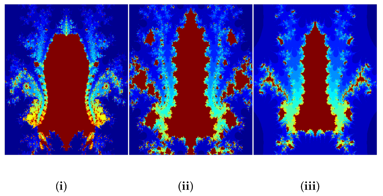
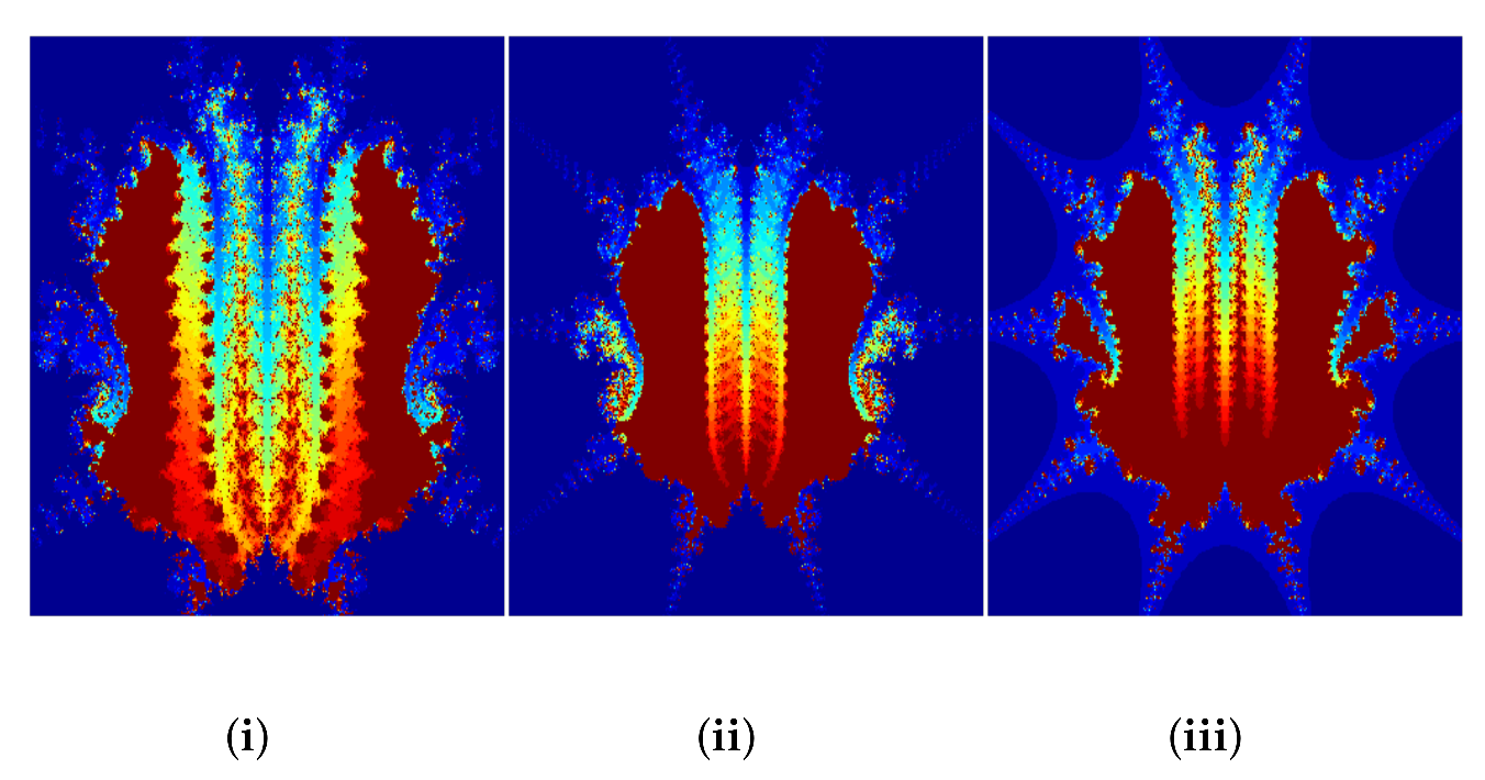
Figure 2.
Cubic Julia sets in (i) Noor-orbit; (ii) Ishikawa-orbit; (iii) Mann-orbit.

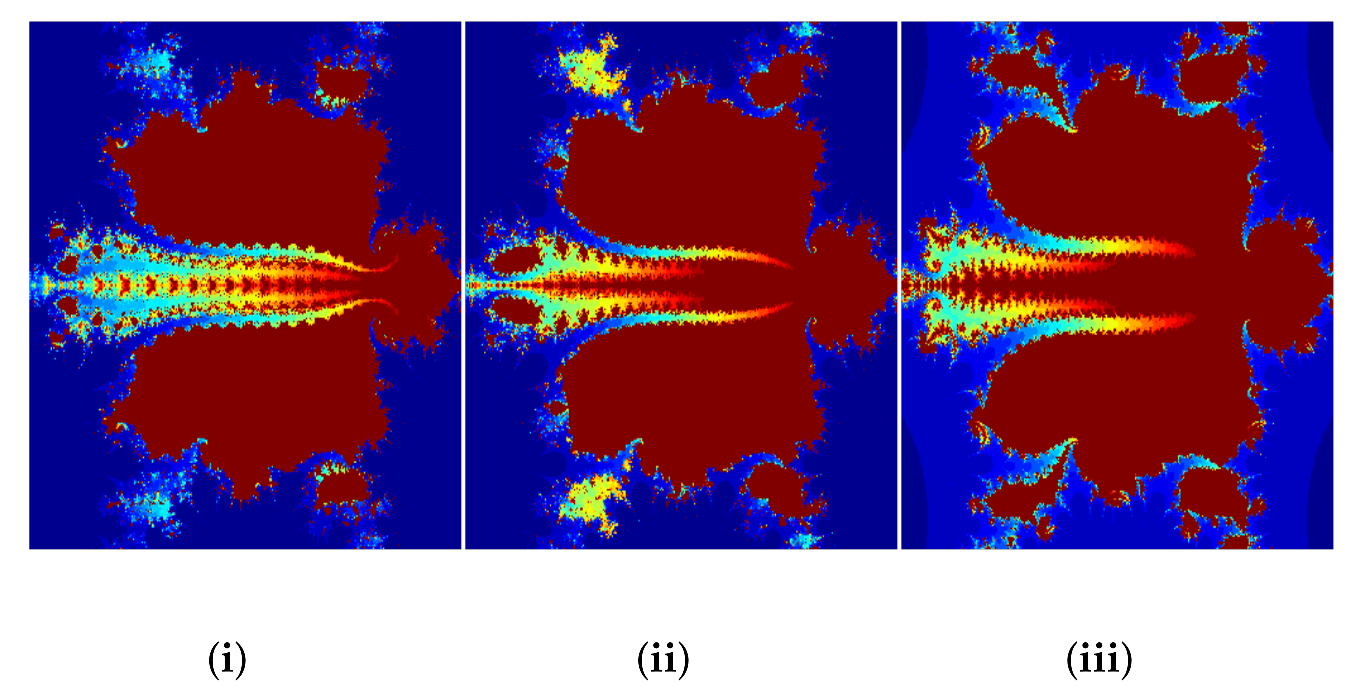
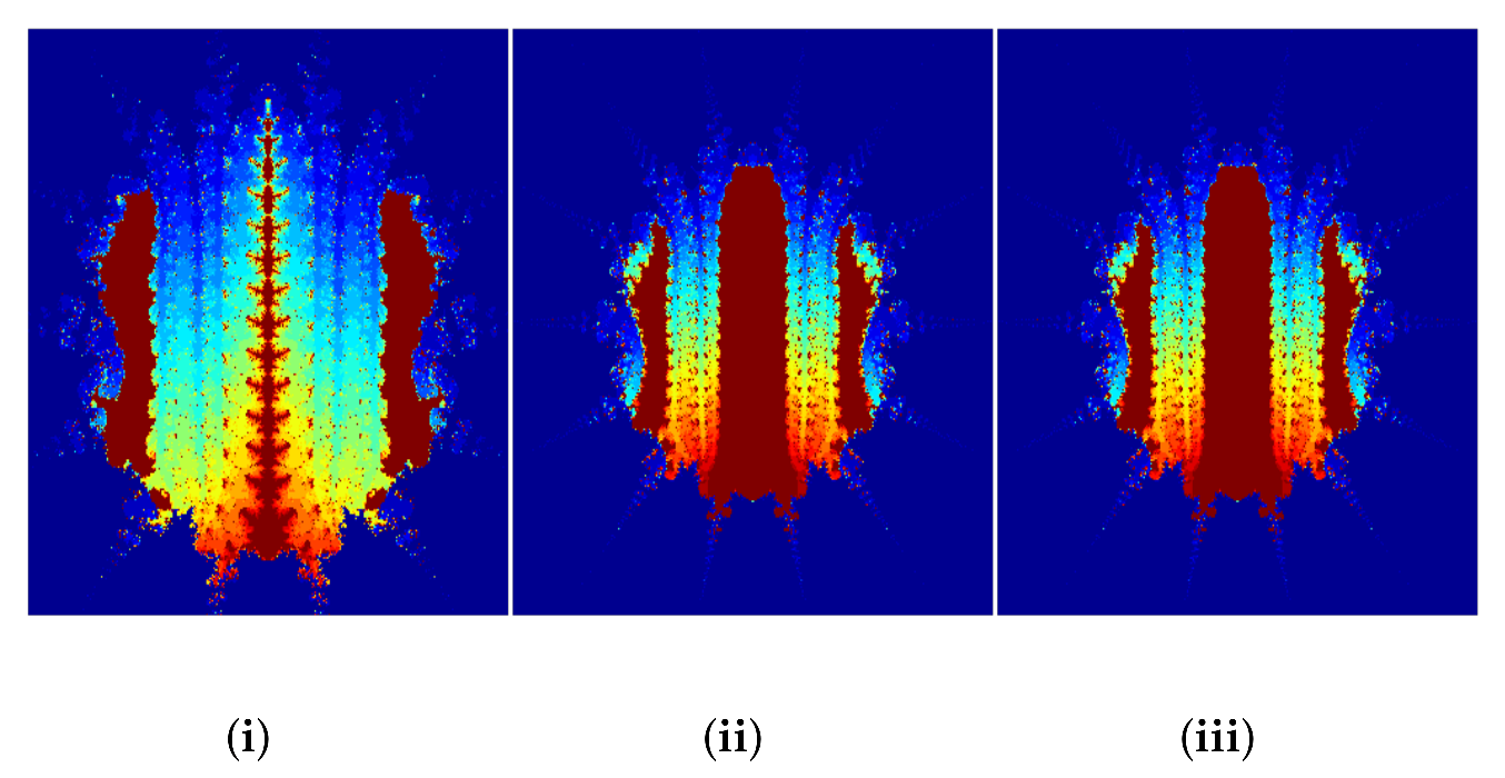
Figure 3.
Cubic Julia sets in (i) Noor-orbit; (ii) Ishikawa-orbit; (iii) Mann-orbit.

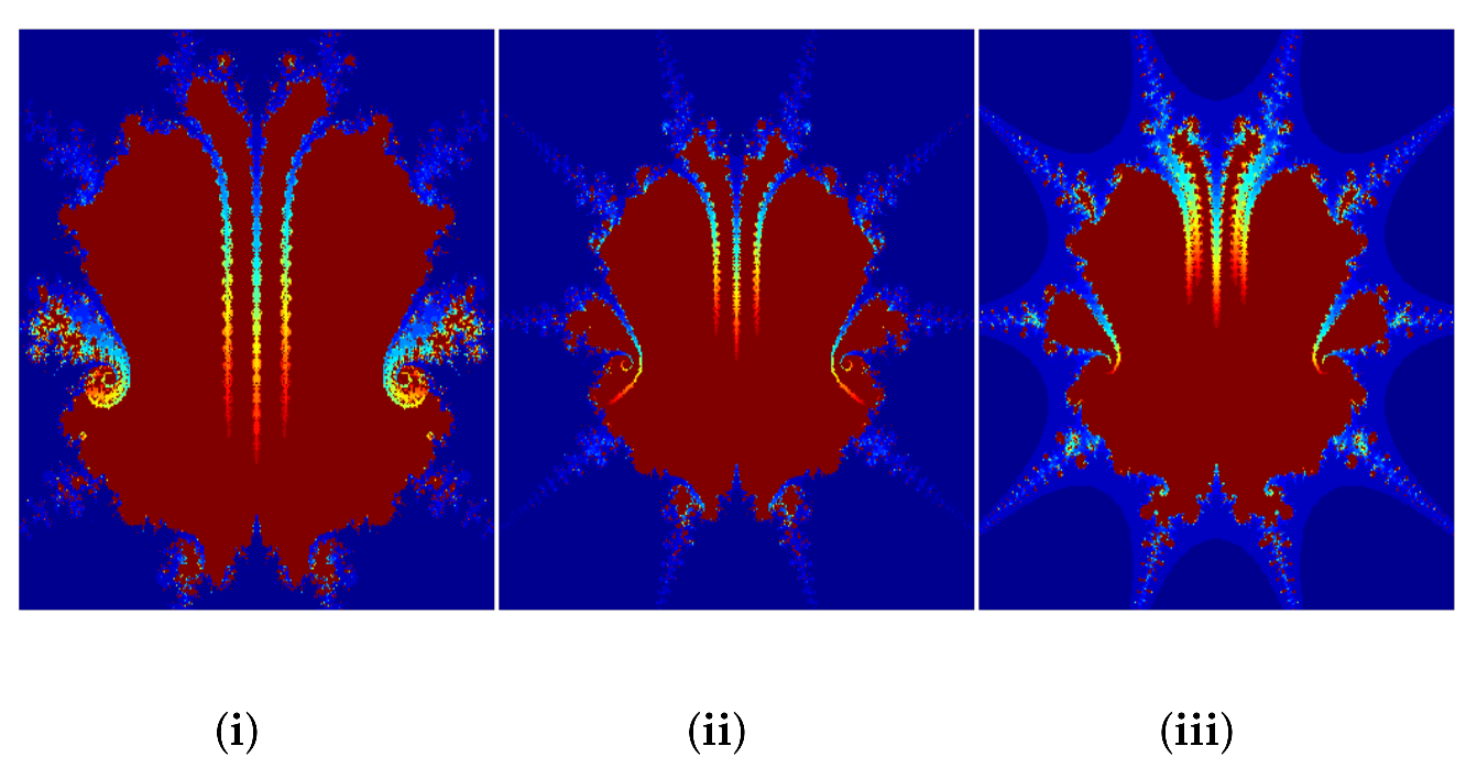
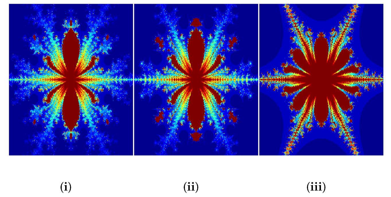
Figure 4.
Quintic Julia sets in (i) Noor-orbit; (ii) Ishikawa-orbit; (iii) Mann-orbit.

Figure 5.
Cubic Julia sets in (i) Noor-orbit; (ii) Ishikawa-orbit; (iii) Mann-orbit.

Figure 6.
Quintic Julia sets in (i) Noor-orbit; (ii) Ishikawa-orbit; (iii) Mann-orbit.

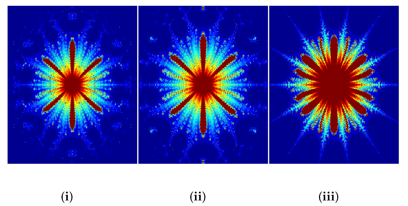
Figure 7.
Septic Julia sets in (i) Noor-orbit; (ii) Ishikawa-orbit; (iii) Mann-orbit.

Figure 8.
Cubic Julia sets in (i) Noor-orbit; (ii) Ishikawa-orbit; (iii) Mann-orbit.

Figure 9.
Quintic Julia sets in (i) Noor-orbit; (ii) Ishikawa-orbit; (iii) Mann-orbit.

Figure 10.
Septic Julia sets in (i) Noor-orbit; (ii) Ishikawa-orbit; (iii) Mann-orbit.

Figure 11.
Higher-order Julia sets in (i) Noor-orbit; (ii) Ishikawa-orbit; (iii) Mann-orbit.

Figure 12.
Cubic Julia sets in (i) Noor-orbit; (ii) Ishikawa-orbit; (iii) Mann-orbit; (iv) Picard-orbit.
Figure 12.
Cubic Julia sets in (i) Noor-orbit; (ii) Ishikawa-orbit; (iii) Mann-orbit; (iv) Picard-orbit.

Figure 13.
Quintic Julia sets in (i) Noor-orbit; (ii) Ishikawa-orbit; (iii) Mann-orbit; (iv) Picard-orbit.
Figure 13.
Quintic Julia sets in (i) Noor-orbit; (ii) Ishikawa-orbit; (iii) Mann-orbit; (iv) Picard-orbit.

Figure 14.
Quintic Julia sets in (i) Noor-orbit; (ii) Ishikawa-orbit; (iii) Mann-orbit; (iv) Picard-orbit.
Figure 14.
Quintic Julia sets in (i) Noor-orbit; (ii) Ishikawa-orbit; (iii) Mann-orbit; (iv) Picard-orbit.

Figure 15.
Septic Julia sets in (i) Noor-orbit; (ii) Ishikawa-orbit; (iii) Mann-orbit; (iv) Picard-orbit.
Figure 15.
Septic Julia sets in (i) Noor-orbit; (ii) Ishikawa-orbit; (iii) Mann-orbit; (iv) Picard-orbit.


Table 1.
The parameters used in Figure 1.
Table 1.
The parameters used in Figure 1.
| a | c | n | |||||||
|---|---|---|---|---|---|---|---|---|---|
| (i) | 1.19802032 | 0.17835 | 0.1675056 | 0.14323409 | 0.11025 | 0.115025 | 0.115025 | 3 | |
| (ii) | 1.19802032 | 0.17835 | 0.1675056 | - | 0.11025 | 0.115025 | - | 3 | |
| (iii) | 1.19802032 | 0.17835 | - | - | 0.11025 | - | - | 3 |
Table 2.
The parameters used in Figure 2.
Table 2.
The parameters used in Figure 2.
| a | c | |||||||
|---|---|---|---|---|---|---|---|---|
| (i) | 1.19802032 | 0.0077835 | 0.1675056 | 0.0814323409 | 0.07101025 | 0.079115025 | 0.078115025 | |
| (ii) | 1.19802032 | 0.0077835 | 0.1675056 | - | 0.07101025 | 0.079115025 | - | |
| (iii) | 1.19802032 | 0.0077835 | - | - | 0.07101025 | - | - |
Table 3.
The parameters used in Figure 3.
Table 3.
The parameters used in Figure 3.
| a | c | |||||||
|---|---|---|---|---|---|---|---|---|
| (i) | 1.0229802032 | −1.89 | 0.077835 | 0.05675056 | 0.0814323409 | 0.000017101025 | 0.79115025 | 0.8115025 |
| (ii) | 1.0229802032 | −1.89 | 0.077835 | 0.05675056 | - | 0.000017101025 | 0.79115025 | - |
| (iii) | 1.0229802032 | −1.89 | 0.077835 | - | - | 0.000017101025 | - | - |
Table 4.
The parameters used in Figure 4.
Table 4.
The parameters used in Figure 4.
| a | c | |||||||
|---|---|---|---|---|---|---|---|---|
| (i) | 1.0229802032 | −1.0089i | 0.077835 | 0.05675056 | 0.0814323409 | 0.000017101025 | 0.79115025 | 0.8115025 |
| (ii) | 1.0229802032 | −1.0089i | 0.077835 | 0.05675056 | - | 0.000017101025 | 0.79115025 | - |
| (iii) | 1.0229802032 | −1.0089i | 0.077835 | - | - | 0.000017101025 | - | - |
| a | c | |||||||
|---|---|---|---|---|---|---|---|---|
| (i) | 1.0229802032 | −1.89i | 0.077835 | 0.05675056 | 0.0814323409 | 0.000017101025 | 0.79115025 | 0.8115025 |
| (ii) | 1.0229802032 | −1.89i | 0.077835 | 0.05675056 | - | 0.000017101025 | 0.79115025 | - |
| (iii) | 1.0229802032 | −1.89i | 0.077835 | - | - | 0.000017101025 | - | - |
| a | c | |||||||
|---|---|---|---|---|---|---|---|---|
| (i) | 6.5 | 0 | 0.0097577835 | 0.11295675056 | 0.00975814323409 | 0.17101025 | 0.115025 | 0.8115025 |
| (ii) | 6.5 | 0 | 0.0097577835 | 0.11295675056 | - | 0.17101025 | 0.115025 | - |
| (iii) | 6.5 | 0 | 0.0097577835 | - | - | 0.17101025 | - | - |
Publisher’s Note: MDPI stays neutral with regard to jurisdictional claims in published maps and institutional affiliations. |
© 2021 by the authors. Licensee MDPI, Basel, Switzerland. This article is an open access article distributed under the terms and conditions of the Creative Commons Attribution (CC BY) license (https://creativecommons.org/licenses/by/4.0/).
Share and Cite
MDPI and ACS Style
Antal, S.; Tomar, A.; Prajapati, D.J.; Sajid, M. Fractals as Julia Sets of Complex Sine Function via Fixed Point Iterations. Fractal Fract. 2021, 5, 272. https://0-doi-org.brum.beds.ac.uk/10.3390/fractalfract5040272
AMA Style
Antal S, Tomar A, Prajapati DJ, Sajid M. Fractals as Julia Sets of Complex Sine Function via Fixed Point Iterations. Fractal and Fractional. 2021; 5(4):272. https://0-doi-org.brum.beds.ac.uk/10.3390/fractalfract5040272
Chicago/Turabian StyleAntal, Swati, Anita Tomar, Darshana J. Prajapati, and Mohammad Sajid. 2021. "Fractals as Julia Sets of Complex Sine Function via Fixed Point Iterations" Fractal and Fractional 5, no. 4: 272. https://0-doi-org.brum.beds.ac.uk/10.3390/fractalfract5040272