Study of Lagrange Points in the Earth–Moon System with Continuation Fractional Potential

Abstract

In this work, the restricted three-body system is studied in the framework of the continuation fractional potential with its application on the Earth–Moon system. With the help of a numerical technique, we obtained thirteen equilibrium points, such that nine of them are collinear while the remaining four are non-collinear points. We found that the collinear points near the smaller primary were shifted outward from the Moon, whereas the points near the bigger primary were shifted towards the Earth as the value of the continuation fractional parameter increased. We analyzed the zero-velocity curves and discussed the perturbation of the continuation fractional potential effect on the possible regions of the motion. We also discussed the linear stability of all the equilibrium points and found that out of thirteen only two were stable. Due to such a prevalence, the continuation fractional potential is a source of significant perturbation, which embodies the lack of sphericity of the body in the restricted three-body problem

1. Introduction

The restricted three-body problem has a great significance in both celestial mechanics and space dynamics, because the N-body problem can be reduced to the perturbed three-body problem in most practical cases, which is more simple than the general N-body problem while maintaining the fundamental dynamical properties of the original system. In the solar system, the Sun–Earth–Moon system and the Sun–Jupiter–infinitesimal body system or Earth–Moon–infinitesimal body system, etc., can be considered spacial cases of the N-body problem [1,2,3,4,5]. There are many factors which affect the motion of celestial bodies, which are called perturbations forces. These forces have motivated some researchers and scientists to review the precision of Newton’s inverse square law and search for new modified potential models.

There are several dynamical features in the context of the perturbed restricted three-body problem which are studied using several types of modified potentials [6,7,8,9,10]. These potentials acquire their importance from the fact that the most celestial bodies in both solar systems and outer space are non-spherical symmetry objects, but they can be considered extended bodies. In addition, the effects of radiation pressure and oblateness have been analyzed in detail [4,11].

The modified or perturbed potentials are not limited to the restricted three-body problem; they also include its reduced versions, two-, four- and five-body problems, etc. The periodic solution of the perturbed two-body problem has been studied using different perturbations methods in [12,13,14].

While in the framework of reduced versions of the restricted three-body problem, the periodic orbits in the perturbed Hill’s model of the three-body problem are calculated under various perturbations in [15]. Furthermore, the geometry of halo and Lissajous orbits, approximated periodic orbits, as well as periodic solutions of circular and elliptic restricted three-, four- and five-body problems with drag forces, are computed by many researchers in [16,17,18,19,20].

We may use an infinitesimal body in the proposed system to analyze the motion of dust grains or spacecraft, specifically in the proximity of an exoplanet. Since the shape of most celestial bodies suffers from a lack of sphericity, this system can be used to obtain rigorous data about the locations of equilibrium points and their stability for the infinitesimal bodies. Recent work in this field is addressed in [21]. The authors studied the influence of a modified gravitational potential ( i.e., that the smaller primary potential is modified by including a term of general relativity) on the location of libration points and Newton–Raphson basins of conservation at a specific value of mass parameter $\mu =0.3$.

In this work, a new formulation for the Earth–Moon system in the framework of the modified Newtonian potential is derived using a continuation fractional potential, where this potential is generalized for a Newtonian potential and includes the effect of the non-sphericity of a primary body (the Earth, for example) which represents a significant perturbation in the restricted three-body problem. In the proposed system, the potential function depends on a non-negative small parameter ($ϵ$). This system acquires its importance from two reasons: first, the potential function has no singularity when this parameter is non-zero; second, the effect of this parameter may play the same role as the zonal harmonic coefficients [14].

Furthermore, we elaborate the similarities and differences between the current work and the publication in [22]. In both works, the restricted three-body problem is the proposed system. However, we assumed that the bigger primary is radiating and the second is a non-spherical body that creates a gravitational field as in a continuation fractional potential in the old work; this model can be applied to study the Sun–Earth system in which the Sun is a radiating body and the Earth is non-spherical. In the current work, by contrast, we assume that the bigger primary suffers from a lack of sphericity and creates the same gravitational field of a continuation fractional potential with no radiation pressure effect, with the potential of the second primary being identified by the point mass potential. Thus, the current model is appropriate for approximating the Earth–Moon system.

This work includes five sections. The literature on the restricted three-body problem is addressed in Section 1. The model description and the surface of zero velocity are constructed in Section 2. The Lagrangian points under the effect of the perturbed parameter of the continuation fractional potential are analyzed in Section 3. The stability of the Lagrangian points is studied in Section 4. Finally, in Section 5, the conclusion is stated.

2. Formulation of the Model

Let us consider the Earth–Moon system in which the Earth is a non-spherical body and its gravitational field is identified by a continuation fractional potential, while the Moon creates a potential as a point mass or spherical body (for details see [14,22]). Thus, we propose that $m_1$ and $m_2$ be the masses of the Earth and the Moon, while the mass of the infinitesimal body is m, which is considered a negligible mass with respect to the Earth and Moon. Both primary bodies (i.e., Earth and Moon) move in circular orbits around their common center of mass under their mutual gravitational potential. The Earth affects both the Moon and infinitesimal bodies through a continuation fractional potential, while the Moon affects the Earth and infinitesimal bodies through a Newton gravitational potential. However, the infinitesimal body does not influence the motion of the Earth or the Moon due to its negligible mass.

Let us normalize also the units of the proposed system in such a way that the separation distance between the Earth and the Moon, the sum of their masses and the gravitational constant G are equal to unity. Therefore, we can denote the mass of the Moon with $\mu =m_2/(m_1+m_2)$, and so the mass of the Earth is $(1-\mu )$. Furthermore, we assume that $OXYZ$ is a synodic reference frame instead of a sidereal frame $O\xi \eta \zeta$, which has the same origin, and the first frame rotates about the $\zeta$-axis with an angular velocity $\omega$. Furthermore, we assume that the primaries are moving in the $XY$ plane and lying on the X-axis. Then, the coordinates of the first, second and infinitesimal bodies in the synodic frame are $(-\mu ,0,0)$, $(1-\mu ,0,0)$ and $(x,y,z)$, respectively (see Figure 1). Hence, the equations of the motion of the infinitesimal body in the synodic frame is given as in [22] by

$$\begin{array}{cc}\ddot{x}-2\omega \dot{y}=\hfill & W_x,\hfill \\ \hfill \ddot{y}+2\omega \dot{x}=& W_y,\hfill \\ \hfill \ddot{z}=& W_z,\hfill \end{array}$$

(1)

where the effective potential $W(x,y,z)$ is given by

$$W(x,y,z)={\displaystyle \frac{{\omega }^2(x^2+y^2)}{2}}+{\displaystyle \frac{(1-\mu )r_1}{r_1^2+ϵ}}+{\displaystyle \frac{\mu }{r_2}},$$

(2)

where $r_1=\left|{\mathbf{r}}_1\right|$ and $r_2=\left|{\mathbf{r}}_2\right|$ are the magnitudes of the distances of the infinitesimal body from the first and second primaries, respectively, which are defined as

$$\begin{array}{cc}\hfill r_1^2=& {(x+\mu )}^2+y^2+z^2,\hfill \\ \hfill r_2^2=& {(x+\mu -1)}^2+y^2+z^2.\hfill \end{array}$$

(3)

Here, $ϵ$ is considered a perturbed parameter, which is derived from the continuation fractional potential, and $\omega$ denotes the perturbed mean motion, with both of them due to the non-spherical shape of the Earth. Furthermore, the functions $W_x$, $W_y$ and $W_z$ denote the first-order partial derivatives of $W(x,y,z)$ with respect to x, y and z, respectively. Thus, we can write

$$\begin{array}{cc}\hfill W_x=& (1-\mu )(x+\mu )\left({\omega }^2-{\displaystyle \frac{r_1^2-ϵ}{r_1{(r_1^2+ϵ)}^2}}\right)+\mu (x+\mu -1)\left({\omega }^2-\frac{1}{r_2^3}\right),\hfill \\ \hfill W_y=& y\left[(1-\mu )\left({\omega }^2-{\displaystyle \frac{r_1^2-ϵ}{r_1{(r_1^2+ϵ)}^2}}\right)+\mu \left({\omega }^2-{\displaystyle \frac{1}{r_2^3}}\right)\right],\hfill \\ \hfill W_z=& z\left[(1-\mu )\left({\omega }^2-{\displaystyle \frac{r_1^2-ϵ}{r_1{(r_1^2+ϵ)}^2}}\right)+\mu \left({\omega }^2-{\displaystyle \frac{1}{r_2^3}}\right)-{\omega }^2\right].\hfill \end{array}$$

(4)

and

$${\omega }^2={\displaystyle \frac{1-ϵ}{{(1+ϵ)}^2}}.$$

(5)

The well-known energy integral of the proposed problem can be obtained by integrating Equation (1) as

$$\begin{array}{c}\hfill 2W(x,y,z)-({\dot{x}}^2+{\dot{y}}^2+{\dot{z}}^2)=C,\end{array}$$

(6)

where C is known as the Jacobi constant. Equation (6) has many features; for example, it can be used to evaluate the zero-velocity curves and identify the areas of permission and prohibition motions of the infinitesimal body.

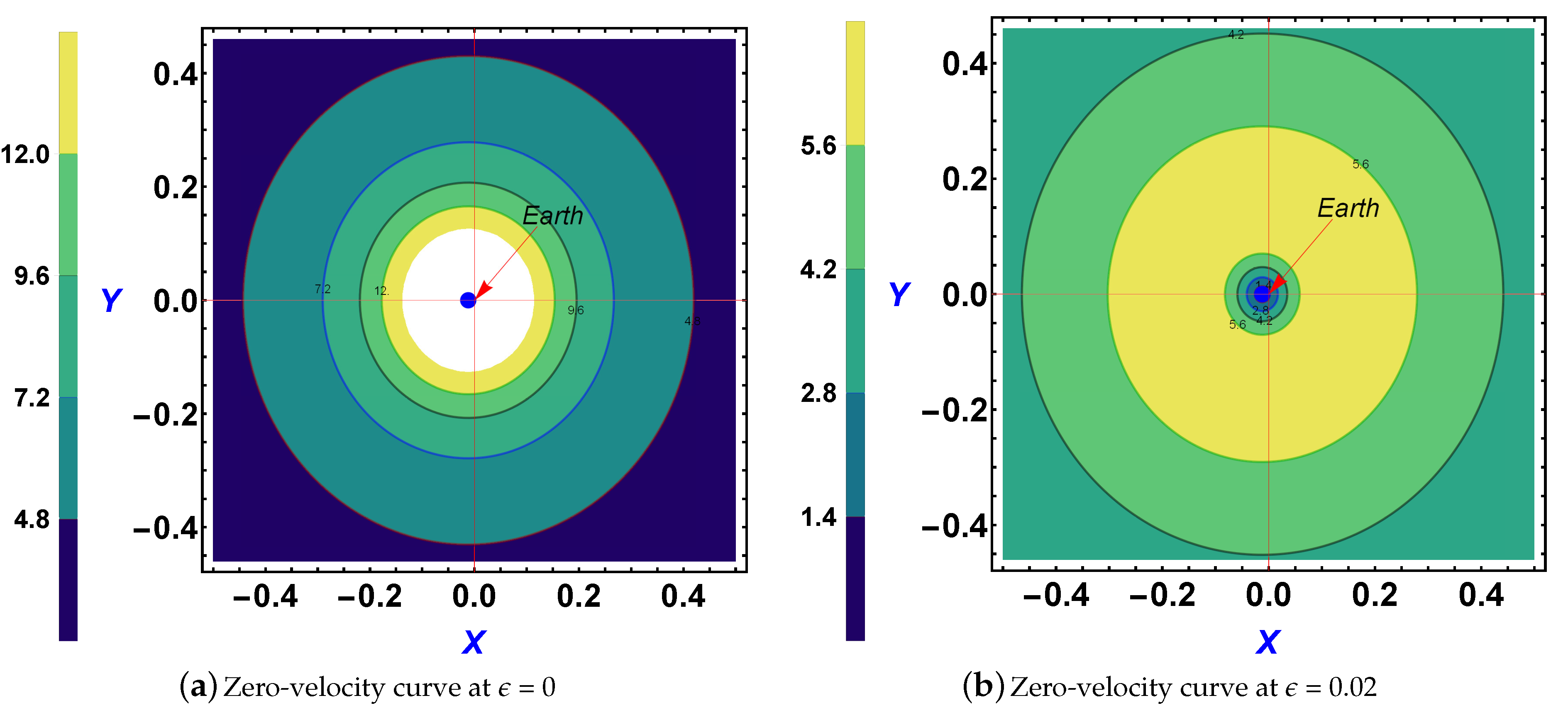
Utilizing Equations (2), (3) and (5) with Equation (6), we can plot zero-velocity curves at various values of the perturbed parameter $ϵ$ shown in Figure 2 and Figure 3. It may be seen that the zero-velocity curve changed due to the continuation fractional potential. The permitted region increased in the interval $0\le ϵ\le 0.02$ and then formed a closed loop at $ϵ=0.04$ around the Moon. Furthermore, in the interval $0.04<ϵ\le 0.1$, the permitted or possible region of motion expanded (see Figure 2a–f). On the other hand, the permitted region of the motion expanded initially, then shrank and assumed an oval-shaped orbit in the interval $0\le ϵ\le 0.1$ around the Earth (see Figure 3a–f).

3. Equilibrium Points

In the framework of dynamical system motion, the locations or positions of equilibrium points are identified when the velocities and accelerations of the bodies are equal to zero. Thereby, the equilibrium points related to the system of Equation (1) can be computed by solving the equations

$$W_x=W_y=W_z=0.$$

(7)

There are two possible solutions for $W_z=0$: either $z\ne 0$ or $z=0$. If $z\ne 0$, and the third sub-equation in Equation (4) is used, we obtain

$$(1-\mu ){\displaystyle \frac{(r_1^2-ϵ)}{r_1{(r_1^2+ϵ)}^2}}=-{\displaystyle \frac{\mu }{r_2^3}}.$$

(8)

The relation in Equation (8) provides a contradiction, as the quantity on the left-hand side will always be positive because $0<\mu <<1$, $(1-\mu )>0$ and $ϵ$ are very small quantities; moreover, $ϵ<<r_1$, whereas on right-hand side the quantity is negative. Therefore, the value of z must be equal to zero; all the equilibrium points will hence always lie on the $XY$ plane. This means that there are no out-of-plane equilibrium points as in the classical case of the unperturbed restricted three-body problem.

The solution of Equation (7) cannot be found analytically due to the complexity of the system. Therefore, with the help of the MATHEMATICA–12 SOFTWARE, we computed thirteen equilibrium points when $ϵ>0$. Among these, nine equilibrium points were collinear and the remaining four were non-collinear points. On the other hand, when $ϵ=0$, we obtained five equilibrium points, and among these, three were collinear and the other two were non–collinear equilibrium points, which provides the same results as the classical case.

3.1. Collinear Equilibrium Points

The collinear equilibrium points can be evaluated when $y=0$ and $z=0$; hence, these points lie on the X-axis. Therefore, after utilizing Equations (4) and (7), we have

$$\begin{array}{c}\hfill (x+\mu )(1-\mu )\left[{\omega }^2-{\displaystyle \frac{{(x+\mu )}^2-ϵ}{(x+\mu ){({(x+\mu )}^2+ϵ)}^2}}\right]+(x+\mu -1)\mu \left[{\omega }^2-{\displaystyle \frac{1}{{(x+\mu -1)}^3}}\right]=0.\end{array}$$

(9)

For a fixed-mass parameter $\mu =0.01215058$ of the Earth–Moon system in Equation (9), it is observed that the collinear equilibrium points depend on the parameter $ϵ$.

In order to avoid the confusion among the notations of the perturbed and the unperturbed Lagrangian points, we would like to direct the attention of the readers to the following acronyms. We denote the classical (or unperturbed) Lagrangian points with ${\tilde{L}}_i,i=1,2,\cdots ,5$, where the perturbed parameter $ϵ=0$, as in

Table 1. Values of unperturbed Lagrangian points.

$\mathit{ϵ}$	${\tilde{\mathit{L}}}_1$	${\tilde{\mathit{L}}}_2$	${\tilde{\mathit{L}}}_3$	${\tilde{\mathit{L}}}_4$	${\tilde{\mathit{L}}}_5$
0.00	(0.836915 ,0.000)	(1.15568 , 0.000)	(−1.00506 , 0.000)	(0.487849 , 0.866025)	(0.487849 , −0.866025)

and Figure 4a. However, the symbols $L_i,i=1,2,\cdots ,9$ are taken for the perturbed collinear Lagrangian points where the perturbed parameter $ϵ\ne 0$, as in

Table 2. Values of perturbed collinear Lagrangian points at different values of the parameter $ϵ$.

$\mathit{ϵ}$	${\mathit{L}}_1$	${\mathit{L}}_2$	${\mathit{L}}_3$	${\mathit{L}}_4$	${\mathit{L}}_5$	${\mathit{L}}_6$	${\mathit{L}}_7$	${\mathit{L}}_8$	${\mathit{L}}_9$
0.02	0.831093	1.16084	−1.00483	0.130074	0.129881	0.12849	−0.152807	−0.152703	−0.154358
0.04	0.824892	1.166615	−1.00459	0.190977	0.190322	0.184949	−0.209338	−.209079	−0.215176
0.06	0.818243	1.171164	−1.00433	0.239697	0.238267	0.226757	−0.25129	−0.250866	−0.263695
0.08	0.811057	1.17731	−1.00406	0.282783	0.28017	0.260753	−0.285508	−0.284907	−0.306405
0.10	0.803214	1.18319	−1.00376	0.322807	0.38457	0.289696	−0.314754	−0.31398	−0.345794

and Figure 4b–f, while the perturbed non-collinear Lagrangian points are termed ${\overline{L}}_i,i=1,2,\cdots ,4$, as in

Table 3. Values of perturbed non-collinear Lagrangian points at different values of parameter $ϵ$.

$\mathit{ϵ}$	${\overline{\mathit{L}}}_1$	${\overline{\mathit{L}}}_2$	${\overline{\mathit{L}}}_3$	${\overline{\mathit{L}}}_4$
0.02	(0.467511 , 0.877454)	(0.467511 , −0.877454)	(−0.022381 , 0.141817)	(−0.022381 , −0.141817)
0.04	(0.446472 , 0.888631)	(0.446472 , −0.888631)	(−0.0329346 , 0.201879)	(−0.0329346 , −0.201879)
0.06	(0.424697 , 0.899536)	(0.424697 , −0.899536)	(−0.0437072 , 0.249391)	(−0.0437072 , −0.249391)
0.08	(0.402148 , 0.910141)	(0.402148 , −0.910141)	(−0.0546412 , 0.290889)	(−0.0546412 , −0.290889)
0.10	(0.378782 , 0.920419)	(0.378782 , −0.920419)	(−0.0656985 , 0.328894)	(−0.0656985 , −0.328894)

and the aforementioned sub-figures.

In this context, we observe that with increases in the value of $ϵ$ the points $L_1$ and $L_2$ slid out of the smaller primary, whereas the point $L_3$ shifted towards the bigger primary. Moreover, the remaining six collinear points were near the common center of the mass of the primaries. When the perturbed parameter $ϵ$ increased, the points slid out from the common center of the primaries’ mass.

3.2. Non-Collinear Equilibrium Points

For the equilibrium points lying in the $XY$ plane, z must be equal to zero. Therefore, from the first two sub-equations in Equation (4), we obtain

$$\begin{array}{cc}\hfill (x+\mu )(1-\mu )\left[{\omega }^2-{\displaystyle \frac{r_1^2-ϵ}{r_1{(r_1^2+ϵ)}^2}}\right]+(x+\mu -1)\mu \left[{\omega }^2-{\displaystyle \frac{1}{r_2^3}}\right]=& 0,\hfill \\ \hfill y(1-\mu )\left[{\omega }^2-{\displaystyle \frac{r_1^2-ϵ}{{(r_1^2+ϵ)}^2}}\right]+y\mu \left[{\omega }^2-{\displaystyle \frac{1}{r_2^3}}\right]=& 0.\hfill \end{array}$$

(10)

Now, solving Equation (10) numerically using the Mathematica software, we obtain four non-collinear points at $ϵ\ne 0$ defined by ${\overline{L}}_1,{\overline{L}}_2,{\overline{L}}_3$ and ${\overline{L}}_4$ (see Table 3), whereas for the classical case at $ϵ=0$, these are defined by ${\tilde{L}}_4$ and ${\tilde{L}}_5$ (see Table 1).

The values of the non-collinear points in the case of the unperturbed restricted three-body problem ($ϵ=0$) are presented in Table 1, while the non-collinear points under the effect of the continuation fractional potential are presented in Table 3. A clear visualization of the collinear and non-collinear libration points are presented in Figure 4. The positions of ${\overline{L}}_1$ and ${\overline{L}}_2$ shifted towards the center of the primaries’ mass, while those of ${\overline{L}}_3$ and ${\overline{L}}_4$ shifted towards the larger primary body.

4. Stability of Locations Point

This section is devoted to analyzing the stability of motion for the infinitesimal body around the locations of equilibrium points by assuming small changes in these locations. Hence, we assumed that the infinitesimal body was displaced very slightly from the exact position of the equilibrium point and acquired a small velocity, such that it would either oscillate around the respective position, at least for a considerable interval of time (before it becomes stable), or rapidly depart from its position (with the body motion being unstable).

Now, we propose that $(x_0,y_0)$ be the exact position of the infinitesimal body at the equilibrium points, and that there is a small displacement in these positions; the new coordinates can be written as $x=x_0+\xi ,y=y_0+\eta$. Thus, we obtain $\dot{x}=\dot{\xi }$, $\dot{y}=\dot{\eta }$, and thus the coordinates of the infinitesimal body and the components of its velocity are $x=x_0+\xi$, $y=y_0+\eta$, $\dot{x}=\dot{\xi }$ and $\dot{y}=\dot{\eta }$, where $\xi$, $\eta$, $\dot{\xi }$ and $\dot{\eta }$ are initially very small quantities. Now, substituting these values in Equation (1) and simplifying with the help of Taylor series expansion about $(x_0,y_0)$ while neglecting higher-order derivative terms and keeping only the first order of $\xi$, $\eta$ and $\zeta$, we obtain

$$\begin{array}{cc}\hfill \ddot{\xi }-2\dot{\eta }=& \xi W_{xx}^0+\eta W_{xy}^0,\hfill \\ \hfill \ddot{\eta }+2\dot{\xi }=& \xi W_{yx}^0+\eta W_{yy}^0,\hfill \end{array}$$

(11)

where $W_{xx}^0,W_{xy}^0,W_{yx}^0$ and $W_{yy}^0$ represent a second-order partial derivative of the potential function $W(x,y,z)$ with respect to x and y, respectively, at $(x_0,y_0)$. In order to solve Equation (11), let us consider

$$\begin{array}{cc}\hfill & \xi =C{e}^{\lambda t},\hfill \\ \hfill & \eta =D{e}^{\lambda t},\hfill \end{array}$$

(12)

where C and D are constants and $\lambda$ is the characteristic parameter of the solution. Substituting the values of Equation (12) into Equation (11) and canceling out the common factor, a system of linear equations is obtained, which is given as

$$\begin{array}{c}\hfill \left({\lambda }^2-W_{xx}^0\right)C+\left(-2\omega \lambda -W_{yx}^0\right)D=0,\\ \hfill \left(2\lambda \omega -W_{yx}^0\right)C+\left({\lambda }^2-W_{yy}^0\right)D=0.\end{array}$$

(13)

Since Equation (13) represents a homogeneous dynamical system, the determinant of the coefficient matrix must be zero for non-trivial solutions; therefore,

$$\left|\begin{array}{cc}{\lambda }^2-W_{xx}^0& -2\omega \lambda -W_{yx}^0\\ 2\lambda \omega -W_{yx}^0& {\lambda }^2-W_{yy}^0\end{array}\right|=0.$$

(14)

Simplifying the above Equation (14), we obtain a characteristic equation in terms of $\lambda$ as

$$\begin{array}{c}\hfill {\lambda }^4+K_1{\lambda }^2+K_2=0,\end{array}$$

(15)

where $K_1=4-W_{xx}^0-W_{yy}^0$ and $K_2=W_{xx}^0{W}_{yy}^0-{\left(W_{xy}^0\right)}^2$. The value of $\lambda$ is called the characteristic roots or eigenvalues of the Equation (15). The solving of Equation (15) gives four roots (${\lambda }_i$, $i=1,2,3,4$) as

$${\lambda }_{1,2,3,4}=\pm \sqrt{{\displaystyle \frac{-K_1\pm \sqrt{K_1^2-4K_2}}{2}}}.$$

(16)

Using the obtained roots in Equation (16), the general solution of the linear differential system with the constant coefficients of Equation (11) can be written as

$$\begin{array}{cc}\hfill \xi \left(t\right)=& C_1{e}^{{\lambda }_{1}t}+C_2{e}^{{\lambda }_{2}t}+C_3{e}^{{\lambda }_{3}t}+C_4{e}^{{\lambda }_{4}t},\hfill \\ \hfill \eta \left(t\right)=& D_1{e}^{{\lambda }_{1}t}+D_2{e}^{{\lambda }_{2}t}+D_3{e}^{{\lambda }_{3}t}+D_4{e}^{{\lambda }_{4}t},\hfill \end{array}$$

(17)

where $C_i$ and $D_i,i=1,2,3,4$ are integral constants.

The value of $D_i$ can be obtained in the form of $C_i$ with the help of linear Equation (13). From Equation (17), we remark that if all characteristic roots ${\lambda }_i,i=1,2,3,4$ of Equation (15) are complex conjugates and there exists at least one root with a positive real part, then the solution $\xi$ and $\eta$ will be unstable. On the other side, if all real parts of the complex roots are negative, then the solutions $\xi$ and $\eta$ will be asymptotically stable. However, if all the characteristic roots are purely imaginary, then the obtained solutions $\xi$ and $\eta$ will be periodic in their structures and hence stable, while if all the characteristic roots are real, then solutions $\xi$ and $\eta$ will be unstable.

We know that the collinear libration points lie on the X-axis, i.e., $y=0$, so that $W_{xy}^0=W_{yx}^0=0$ and Equation (15) takes the form

$$\begin{array}{c}\hfill {\lambda }^4+K_1^{*}{\lambda }^2+K_2^{*}=0,\end{array}$$

(18)

where $K_1^{*}=K_1$ and $K_2^{*}=W_{xx}^0{W}_{yy}^0$, and the solution of Equation (18) gives the characteristic roots in the case of collinear points as

$$\begin{array}{c}\hfill {\lambda }_{1,2,3,4}=\pm \sqrt{{\displaystyle \frac{-K_1^{*}\pm \sqrt{K_1^{*2}-4K_2^{*}}}{2}}}.\end{array}$$

(19)

Now the discriminant $D^{\prime }=K_1^{*2}-4K_2^{*}$ of Equation (19) can be used to find out the nature of the characteristic roots as

• Case (i) $K_1^{*2}-4K_2^{*}\le 0$, then unstable;
• Case (ii) $K_1^{*2}-4K_2^{*}>0$, then stable.

For the collinear points $L_i,i=1,2,\cdots ,9$ at each value of the parameter $ϵ$, the characteristic roots are complex, having a real part with the opposite sign. Therefore, for each value of $ϵ$, all collinear points are unstable. Since each two exponential terms have opposite signs, all collinear libration points are saddle points.

We found that all characteristic roots of Equation (15) are purely imaginary, and they provide the periodic solutions corresponding to the triangular libration points ${\overline{L}}_1$ and ${\overline{L}}_2$. Thus, ${\overline{L}}_1$ and ${\overline{L}}_2$ are stable and both are the center for all values of $ϵ$, while the libration points ${\overline{L}}_3$ and ${\overline{L}}_4$ are unstable due to presence of a positive real part in the characteristic roots for each value of $ϵ$.

5. Conclusions and Discussion

We considered a modified restricted three-body problem in the framework of the continuation fractional potential with its application on the Earth–Moon system to analyze the equilibrium points and their linear stability. In fact, we introduced a new type of force potential in the circular restricted three-body problem (CR3BP). The methods of analysis employed in the conventional CR3BP were applied to the new type of force potential. In the proposed study, the motion of infinitesimal mass was studied on the assumption that the first primary is a non–symmetric body and its gravitational field is identified by a continuation fractional potential effect, while the potential of a second primary is identified by the point mass potential.

With the help of a numerical technique, we obtained thirteen equilibrium points; among these, nine were collinear libration points $(L_i,i=1,2,3,\cdots ,9)$ and four were non-collinear libration points $({\overline{L}}_i,i=1,2,3,4)$. We discussed the linear stability of all the equilibrium points and found that the nine collinear points were unstable, while the non-collinear points ${\overline{L}}_1$ and ${\overline{L}}_2$ were center points and hence were stable, whereas the other two points, ${\overline{L}}_3$ and ${\overline{L}}_4$, were unstable. In brief, out of thirteen points, there were only two stable equilibrium points.

Furthermore, we also discussed the effect of perturbation due to the continuation fractional effect on the possible regions of the motion. The zero-velocity curves were drawn around the Moon and Earth separately to show the variation in the regions of permitted and prohibited motions. We found that the permitted region in the vicinity of the Moon increased in the interval $0\le ϵ\le 0.02$ and then formed a closed loop when $ϵ=0.04$. Again, in the interval $0.04<ϵ\le 0.1$, the permitted region was expanded. By contrast, the zero–velocity curves around the Earth (i.e., the permitted regions of motion in the vicinity of the Earth) first expanded, then shrank and formed an oval–shaped orbit in the interval $0\le ϵ\le 0.1$.

In this work, a new formulation for the Earth–Moon system in the framework of the modified Newtonian potential was constructed using a continuation fractional potential, where this potential is generalized for a Newtonian potential and includes the effect of the non-sphericity of the primary body (the Earth, for example). Furthermore, we discovered that the effect of the continuation fractional parameter which identifies the non-sphericity of larger primaries provides a greater number of equilibrium points apart from the classical five Lagrangian points. Then, we discussed the stability of these points.