Analytical and Numerical Solutions for a Kind of High-Dimensional Fractional Order Equation

Abstract

In this paper, a (4+1)-dimensional nonlinear integrable Fokas equation is studied. It is rarely studied because the order of the highest-order derivative term of this equation is higher than the common generalized (4+1)-dimensional Fokas equation. Firstly, the (4+1)-dimensional time-fractional Fokas equation with the Riemann–Liouville fractional derivative is derived by the semi-inverse method and variational method. Further, the symmetry of the time-fractional equation is obtained by the fractional Lie symmetry analysis method. Based on the symmetry, the conservation laws of the time fractional equation are constructed by the new conservation theorem. Then, the $\left(\frac{G^{\prime }}{G}\right)$-expansion method is used here to solve the equation and obtain the exact traveling wave solutions. Finally, the spectral method in the spatial direction and the Gr$\ddot{u}$nwald–Letnikov method in the time direction are considered to obtain the numerical solutions of the time-fractional equation. The numerical solutions are compared with the exact solutions, and the error results confirm the effectiveness of the proposed numerical method.

1. Introduction

Due to the dimensions of equations increasing, which causes difficulties in the analysis and calculation of high-dimensional partial differential equations, there are more studies on low-dimensional problems than on high-dimensional problems. However, the real world is (3+1)-dimensional, thus high-dimensional equations have important applications in real-world problems [1,2,3]. For the past few years, more and more scholars have begun to pay attention to high-dimensional integrable equations in the integrable field. These equations are mathematical models that can describe some complex physical phenomena in physics, ocean process, engineering, biology, chemistry, nonlinear optics and so on. Now, the research of high-dimensional problems mainly focuses on the integer order. Many scholars are devoted to the study of the exact solutions of integer-order high-dimensional problems. These exact solutions have rich physical meanings and can describe some physical phenomena that cannot be observed easily. In recent years, the theory of fractional calculus has developed rapidly [4,5,6], and it has been applied to various fields, such as viscoelastic mechanics, biology, signal and image processing, machinery, physics and other fields. The fractional calculus has great significance for us to observe and study these practical problems because the fractional-order equations can describe complex problems that integer order equations cannot. So it is necessary to study some useful properties and solutions of the fractional order high-dimensional equation. Motivated by the above considerations, in this paper, a (4+1)-dimensional time fractional Fokas equation is derived and studied.

A popular (4+1)-dimensional research issue is a common generalized Fokas equation. It is generated by extending the Lax pair of the low-dimensional Kadomtsev–Petviashvili equation and Davey–Stewartson equation to higher dimensions [7]. It is mainly used to describe the interaction between elastic and inelastic internal waves. The common generalized Fokas equation is as follows:

$${\left(4u_t-u_{x_1{x}_1{x}_2}+u_{x_2{x}_2{x}_2}+12u{u}_{x_2}\right)}_{x_1}-6u_{y_1{y}_2}=0.$$

(1)

This is a nonlinear partial differential equation with four variables $x_1,x_2,y_1,y_2$ in space direction, one variable t in time direction and a fourth derivative term. A similar equation to be introduced in this paper is produced together with the common generalized Fokas equation, but it is rarely studied because it is more complex, and its form is as follows:

$$\begin{array}{c}16u_{t{x}_2}-u_{x_1{x}_1{x}_1{x}_1}-u_{x_2{x}_2{x}_2{x}_2}+6u_{x_1{x}_1{x}_2{x}_2{x}_2}-12{\left(u^2\right)}_{x_2{x}_2}\hfill \\ \hfill +12{\left(u^2\right)}_{x_1{x}_1}-24u_{y_1{y}_1}+24u_{y_2{y}_2}=0,\end{array}$$

(2)

where $x_1,x_2,y_1,y_2\in R^4,t\in [0,T].$ This is a fifth-order nonlinear integrable partial differential equation with four variables $x_1,x_2,y_1,y_2$ in space direction and one variable t in time direction. Compared with Equation (1), Equation (2) is more complicated, so it is more difficult to study Equation (2).

As far as we all know, Equation (2) has hardly been studied and has not been extended to the time-fractional form. In this paper, the time-fractional form of Equation (2) is studied; the time-fractional form of Equation (2) can be derived for the first time by using the semi-inverse method and the variational method [8]. Because the Kadomtsev–Petviashvili equation and Davey–Stewartson equation have important physical applications in describing surface waves and internal waves in channels with different depths and widths, respectively, this (4+1)-dimensional time fractional Fokas equation can be used to represent many complex nonlinear phenomena in ocean engineering, shallow water waves, fluid mechanics, plasma physics and other fields. We mainly study the symmetry, conservation laws, exact solutions and numerical solutions of this equation.

The symmetry and conservation laws of partial differential equations play an important role in the study of integrability and solutions of partial differential equations [9,10], and it can explain various physical phenomena described by partial differential equations. At first, the Noether theorem [11] provides us with a method of constructing the conservation laws of an integer order partial differential equation. This method establishes the relationship between conservation laws and the symmetry of partial differential equations. However, this approach requires that they are Euler–Lagrange equations. For fractional partial differential equations, we can use the extended Noether theorem to construct the conservation laws [12,13,14], but this method also requires the fractional partial differential equations to satisfy the Lagrangian. Recently, some research has been conducted, where, based on the new conservation law [15], the fractional generalization of Noether operators can be used to obtain the conservation laws of the time-fractional partial differential equation, which does not require the fractional partial differential equation to have the Lagrangian [16]. In this paper, the symmetry property of the time fractional (4+1)-dimensional partial differential equation can be obtained by using Lie symmetry analysis, and the new conservation theorem (Lie points symmetry combined adjoint equations) are considered to obtain the conservation laws of the (4+1)-dimensional time-fractional Fokas equation.

The exact solutions of Equation (1) have been studied by many scholars using different methods. The main methods include the exponential function method, modified tanh-coth method, extended Jacobian elliptic function method, $\left(\frac{G^{\prime }}{G}\right)$-expansion method, extended F-expansion method, extended simplest function method, modified simplest function method, simplified Hirota method and Lie group method. Using the above methods, traveling wave solutions, multi-soliton solutions, soliton solutions, periodic wave solutions, rouge wave and lump wave solutions, V-type solitary wave solutions, breather wave solutions and rational solutions in the determinant form can be obtained [17,18,19,20,21,22,23]. Influenced by the analysis of the exact solutions of the Equation (1), for the exact solutions of the (4+1)-dimensional time-fractional equation, we adopt the $\left(\frac{G^{\prime }}{G}\right)$-expansion method [24,25]. We can obtain several exact traveling wave solutions, which we hope to enrich the dynamic behaviors of high-dimensional nonlinear evolution equations. This method is mainly used to find traveling wave solutions of nonlinear evolution equations. Its advantage is that it can transform partial differential equations into ordinary differential equations for solving equations, simplifying the calculation. This method is very effective for solving high-dimensional nonlinear problems in mathematical physics. Some research can be studied from these articles [26,27,28,29,30].

At present, there are few numerical solutions for (4+1)-dimensional partial differential equations. Bi et al. numerically solved the (4+1)-dimensional anomalous diffusion equation by using the alternating direction method [31]. However, this method is suitable for parabolic equations, but not for other types of partial differential equations. In addition, the finite difference method, finite element method and iterative algorithms for stochastic systems [32] need a lot of calculation to deal with high-dimensional problems, which brings great difficulties to the computer. For the numerical solutions of (3+1)-dimensional seismic waves, as early as 1998, Takashi et al. proposed a numerical method [33,34], which is the spectral method in the spatial direction and the finite difference method in the time direction. Recently, Sun and Wang et al. used this method to numerically calculate the (3+1)-dimensional seismic wave, and compared it with the finite difference method [35,36,37]. They found that the accuracy is improved. The advantage of this method is that it can calculate the equations in each spatial direction and time direction discretely. So it can greatly reduce the amount of calculation compared with the classical finite difference method and finite element method. Inspired by this, we apply it to the (4+1)-dimensional time fractional Fokas equation. The numerical solutions obtained by the considered method is satisfactory and this method may provide a new technique for numerically solving such (4+1)-dimensional high-dimensional equations.

The rest of this article is organized as follows. In Section 2, the semi-inverse method and the variational approach are used to derive the (4+1)-dimensional time fractional Fokas equation. In Section 3, we make use of Lie symmetry analysis to study the symmetry of the time-fractional equation, and we construct the conservation laws of the equation by the new conservation theorem [38,39,40,41,42,43,44]. In Section 4, the exact solutions of the time fractional equation are given by using the $\left(\frac{G^{\prime }}{G}\right)$-expansion method. In Section 5, the time-fractional equation is numerically solved by the spectral method in the spatial direction and the Gr$\ddot{u}$nwald–Letnikov method [45,46] in the time direction. Then, we have some discussions between the exact solutions and numerical solutions. Finally, some conclusions are given in Section 6.

2. Derivation of the (4+1)-Dimensional Time Fractional Fokas Equation

In this section, a (4+1)-dimensional time-fractional Fokas equation in the sense of the Riemann–Liouville fractional derivative is derived by the semi-inverse method and the variational approach. An integer-order (4+1)-dimensional Fokas equation is

$$\begin{array}{c}16u_{t{x}_2}-u_{x_1{x}_1{x}_1{x}_1}-u_{x_2{x}_2{x}_2{x}_2}+6u_{x_1{x}_1{x}_2{x}_2{x}_2}\hfill \\ \hfill -12{\left(u^2\right)}_{x_2{x}_2}+12{\left(u^2\right)}_{x_1{x}_1}-24u_{y_1{y}_1}+24u_{y_2{y}_2}=0.\end{array}$$

(3)

The derivation of the (4+1)-dimensional time-fractional Fokas equation is as follows.

Introducing a potential function $v=v(x_1,x_2,y_1,y_2,t)$ and $u=v_{x_2}$, the subscript of v represents the partial derivatives of v with respect to the variable $x_2$, so the potential equation of Equation (3) can be written as

$$\begin{array}{c}16v_{x_{2}t{x}_2}-v_{x_2{x}_1{x}_1{x}_1{x}_1}-v_{x_2{x}_2{x}_2{x}_2{x}_2}+6v_{x_2{x}_1{x}_1{x}_2{x}_2{x}_2}\hfill \\ \hfill -12{\left(u^2\right)}_{x_2{x}_2}+12{\left(u^2\right)}_{x_1{x}_1}-24v_{x_2{y}_1{y}_1}+24v_{x_2{y}_2{y}_2}=0.\end{array}$$

(4)

The functional form of Equation (4) is as follows:

$$\begin{array}{cc}\hfill J\left(v\right)& ={\int }_{R}d{x}_2{\int }_{X_1}d{x}_1{\int }_{Y_1}d{y}_1{\int }_{Y_2}d{y}_2{\int }_{T}dt\{v\left[16c_1{v}_{x_{2}t{x}_2}-c_2{v}_{x_2{x}_1{x}_1{x}_1{x}_1}\right.\hfill \\ & -c_3{v}_{x_2{x}_2{x}_2{x}_2{x}_2}+6c_4{v}_{x_2{x}_1{x}_1{x}_2{x}_2{x}_2}-12c_5{\left(u^2\right)}_{x_2{x}_2}+12c_6{\left(u^2\right)}_{x_1{x}_1}\hfill \\ & \left.-24c_7{v}_{x_2{y}_1{y}_1}+24c_8{v}_{x_2{y}_2{y}_2}\right]\},\hfill \end{array}$$

(5)

where the coefficients $c_i(i=1,2,...,8)$ are the undetermined Lagrange multipliers. A new integral is obtained by integrating by parts of the above equation with considering the conditions that ${\left(u^2\right)}_{x_2{x}_2},{\left(u^2\right)}_{x_1{x}_1}$ are fixed functions and $v_{x_2}{|}_R=v_{x_2}{{|}_{X_1}=v_{x_2}|}_{Y_1}=$ $v_{x_2}{{|}_{Y_2}=v_{x_2}|}_T=0$. Then using the variation of the new integral, we integrate by parts for each term of the new integral under the variational optimal condition $\delta J\left(v\right)=0$, so we have

$$\begin{array}{c}\hfill 32c_1{v}_{x_{2}t{x}_2}-2c_2{v}_{x_2{x}_1{x}_1{x}_1{x}_1}-2c_3{v}_{x_2{x}_2{x}_2{x}_2{x}_2}+12c_4{v}_{x_2{x}_1{x}_1{x}_2{x}_2{x}_2}\\ \hfill -12c_5{\left(u^2\right)}_{x_2{x}_2}+12c_6{\left(u^2\right)}_{x_1{x}_1}-48c_7{v}_{x_2{y}_1{y}_1}+48c_8{v}_{x_2{y}_2{y}_2}=0.\end{array}$$

(6)

We know Equation (6) is equal to Equation (4), so by comparing these two equations, we obtain the constant multipliers $c_1=c_2=c_3=c_4=c_7=c_8=\frac{1}{2},c_5=c_6=1$. Substituting the values of $c_i(i=1,2,...,8)$ into Equation (5), we obtain the Lagrangian form of Equation (3):

$$\begin{array}{cc}\hfill & L(v,v_{x_1},v_{x_2},v_{y_1},v_{y_2},v_t,v_{x_2{x}_2},v_{x_2{y}_1},v_{x_2{y}_2},v_{x_2{x}_1{x}_1{x}_1},v_{x_2{x}_2{x}_2{x}_2},v_{x_2{x}_1{x}_2{x}_2{x}_2})\hfill \\ & =-8v_t{v}_{x_2{x}_2}+\frac{1}{2}{v}_{x_1}{v}_{x_2{x}_1{x}_1{x}_1}+\frac{1}{2}{v}_{x_2}{v}_{x_2{x}_2{x}_2{x}_2}-3v_{x_2}{v}_{x_2{x}_1{x}_1{x}_2{x}_2}\hfill \\ & -12{\left(u^2\right)}_{x_2{x}_2}v+12{\left(u^2\right)}_{x_1{x}_1}v+12v_{y_1}{v}_{x_2{y}_1}-12v_{y_2}{v}_{x_2{y}_2}.\hfill \end{array}$$

(7)

Similarly, the time-fractional form of Equation (3) has the following Lagrangian form:

$$\begin{array}{cc}\hfill & F(v,v_{x_1},v_{x_2},v_{y_1},v_{y_2},D_t^{\alpha }v,v_{x_2{x}_2},v_{x_2{y}_1},v_{x_2{y}_2},v_{x_2{x}_1{x}_1{x}_1},v_{x_2{x}_2{x}_2{x}_2},v_{x_2{x}_1{x}_2{x}_2{x}_2})\hfill \\ & =-8D_t^{\alpha }v{v}_{x_2{x}_2}+\frac{1}{2}{v}_{x_1}{v}_{x_2{x}_1{x}_1{x}_1}+\frac{1}{2}{v}_{x_2}{v}_{x_2{x}_2{x}_2{x}_2}-3v_{x_2}{v}_{x_2{x}_1{x}_1{x}_2{x}_2}\hfill \\ & -12{\left(u^2\right)}_{x_2{x}_2}v+12{\left(u^2\right)}_{x_1{x}_1}v+12v_{y_1}{v}_{x_2{y}_1}-12v_{y_2}{v}_{x_2{y}_2},\hfill \end{array}$$

(8)

where $D_t^{\alpha }$ is the Riemann–Liouville fractional derivative operator [40].

Consequently, the functional form of (4+1)-dimensional time-fractional Fokas equation is as follows:

$$\begin{array}{cc}\hfill J\left(v\right)=& {\int }_{R}d{x}_2{\int }_{X_1}d{x}_1{\int }_{Y_1}d{y}_1{\int }_{Y_2}d{y}_2{\int }_T{\left(dt\right)}^{\alpha }F(v,v_{x_1},v_{x_2},v_{y_1},v_{y_2},D_t^{\alpha }v,\hfill \\ & v_{x_2{x}_2},v_{x_2{y}_1},v_{x_2{y}_2},v_{x_2{x}_1{x}_1{x}_1},v_{x_2{x}_2{x}_2{x}_2},v_{x_2{x}_1{x}_2{x}_2{x}_2}),\hfill \end{array}$$

(9)

where ${\int }_a^t{\left(d\tau \right)}^{\alpha }f\left(\tau \right)=\alpha {\int }_a^{t}d\tau {(t-\tau )}^{\alpha }f\left(\tau \right)$.

Giving the relation of integrating by parts [47]:

$$\begin{array}{c}\hfill {\int }_a^b{\left(d\tau \right)}^{\alpha }f\left(t\right)D_t^{\alpha }g\left(t\right)=\mathrm{\Gamma }(1+\alpha )\left[{g\left(t\right)f\left(t\right)|}_a^b-{\int }_a^b{\left(dt\right)}^{\alpha }g\left(t\right)D_t^{\alpha }f\left(t\right)\right],f\left(t\right),g\left(t\right)\in [a,b].\end{array}$$

Integrating by parts for Equation (9), making use of the above relation and variational optimal condition $\delta J\left(v\right)=0$, the Euler–Lagrangian equation of (4+1)-dimensional time-fractional Fokas equation can be given as follows:

$$\begin{array}{cc}\hfill & \left(\frac{\partial F}{\partial v}\right)·v+\left(\frac{\partial F}{\partial v_{x_1}}\right)·v_{x_1}+\left(\frac{\partial F}{\partial v_{x_2}}\right)·v_{x_2}+\left(\frac{\partial F}{\partial v_{y_1}}\right)·v_{y_1}+\left(\frac{\partial F}{\partial v_{y_2}}\right)·v_{y_2}\hfill \\ & +\left(\frac{\partial F}{\partial D_t^{\alpha }v}\right)·D_t^{\alpha }v+\left(\frac{\partial F}{\partial v_{x_2{x}_2}}\right)·v_{x_2{x}_2}+\left(\frac{\partial F}{\partial v_{x_2{y}_1}}\right)·v_{x_2{y}_1}\hfill \\ & +\left(\frac{\partial F}{\partial v_{x_2{y}_2}}\right)·v_{x_2{y}_2}+\left(\frac{\partial F}{\partial v_{x_2{x}_1{x}_1{x}_1}}\right)·v_{x_2{x}_1{x}_1{x}_1}+\left(\frac{\partial F}{\partial v_{x_2{x}_2{x}_2{x}_2}}\right)·v_{x_2{x}_2{x}_2{x}_2}\hfill \\ & +\left(\frac{\partial F}{\partial v_{x_2{x}_1{x}_1{x}_2{x}_2}}\right)·v_{x_2{x}_1{x}_1{x}_2{x}_2}=0.\hfill \end{array}$$

(10)

By substituting Equation (8) into Equation (10) and making use of the fractional potential function $D_{x_2}^{\alpha }v(x_1,x_2,y_1,y_2,t)=u(x_1,x_2,y_1,y_2,t)$, the (4+1)-dimensional time-fractional Fokas equation can be obtained:

$$\begin{array}{cc}\hfill & 16D_t^{\alpha }{u}_{x_2}-u_{x_1{x}_1{x}_1{x}_1}-u_{x_2{x}_2{x}_2{x}_2}+6u_{x_1{x}_1{x}_2{x}_2{x}_2}-12{\left(u^2\right)}_{x_2{x}_2}\hfill \\ & +12{\left(u^2\right)}_{x_1{x}_1}-24u_{y_1{y}_1}+24u_{y_2{y}_2}=0.\hfill \end{array}$$

(11)

Equation (11) is the (4+1)-dimensional time-fractional Fokas equation in the sense of the Riemann–Liouville derivative. So $D_t^{\alpha }u$ can be defined as [40]

$$\begin{array}{c}\hfill D_t^{\alpha }u=\left\{\begin{array}{cc}\frac{1}{\mathrm{\Gamma }(n-\alpha )}\frac{{\partial }^n}{\partial t^n}{\int }_0^t{(t-s)}^{n-\alpha -1}u(x_1,x_2,y_1,y_2,s)ds,\hfill & n-1<\alpha <n,\hfill \\ \frac{{\partial }^{n}u}{\partial t^n},\hfill & \alpha =n.\hfill \end{array}\right.\end{array}$$

where $\mathrm{\Gamma }\left(x\right)$ is a gamma function.

3. Analysis of the Symmetry and Conservation Laws for the (4+1)-Dimensional Time-Fractional Fokas Equation

In this section, the Lie symmetry analysis and the new conservation theorem are used to study the symmetry and conservation laws of the (4+1)-dimensional time-fractional Fokas equation.

3.1. Analysis of the Lie Symmetry for the (4+1)-Dimensional Time-Fractional Fokas Equation

The (4+1)-dimensional time-fractional Fokas equation here has five variables $x_1,x_2,y_1,y_2,$

t, giving some infinitesimal transformations as follows:

Infinitesimal transformation of each variable:

$$\begin{array}{cc}\hfill x_1^{*}& =x_1+ϵ{\xi }_1(x_1,x_2,y_1,y_2,t,u)+o\left({ϵ}^2\right),\hfill \\ \hfill x_2^{*}& =x_2+ϵ{\xi }_2(x_1,x_2,y_1,y_2,t,u)+o\left({ϵ}^2\right),\hfill \\ \hfill y_1^{*}& =y_1+ϵ{\xi }_3(x_1,x_2,y_1,y_2,t,u)+o\left({ϵ}^2\right),\hfill \\ \hfill y_2^{*}& =y_2+ϵ{\xi }_4(x_1,x_2,y_1,y_2,t,u)+o\left({ϵ}^2\right),\hfill \\ \hfill t^{*}& =t+ϵ\tau (x_1,x_2,y_1,y_2,t,u)+o\left({ϵ}^2\right),\hfill \\ \hfill u^{*}& =u+ϵ\eta (x_1,x_2,y_1,y_2,t,u)+o\left({ϵ}^2\right),\hfill \end{array}$$

(12)

where $ϵ\ll 1$ is a group parameter, ${\xi }_1,{\xi }_2,{\xi }_3,{\xi }_4,\tau ,\eta$ are infinitesimal parameters. The infinitesimal transformations of the partial derivatives of u with respect to different variables are

$$\begin{array}{cc}\hfill \frac{\partial u^{*}}{\partial x_1^{*}}& =\frac{\partial u}{\partial x_1}+ϵ{\eta }^{x_1}(x_1,x_2,y_1,y_2,t,u)+o\left({ϵ}^2\right),\hfill \\ \hfill \frac{\partial u^{*}}{\partial x_2^{*}}& =\frac{\partial u}{\partial x_2}+ϵ{\eta }^{x_2}(x_1,x_2,y_1,y_2,t,u)+o\left({ϵ}^2\right),\hfill \\ \hfill \frac{\partial u_{x_2}^{*}}{\partial t^{*\alpha }}& =\frac{{\partial }^{\alpha }{u}_{x_2}}{\partial t^{\alpha }}+ϵ{\eta }^{\alpha ,t}(x_1,x_2,y_1,y_2,t,u)+o\left({ϵ}^2\right),\hfill \\ \hfill \frac{\partial u^{*}}{\partial x_1^{{*}^2}}& =\frac{\partial u}{\partial x_1^2}+ϵ{\eta }^{x_1{x}_1}(x_1,x_2,y_1,y_2,t,u)+o\left({ϵ}^2\right),\hfill \\ \hfill \frac{\partial u^{*}}{\partial x_2^{{*}^2}}& =\frac{\partial u}{\partial x_2^2}+ϵ{\eta }^{x_2{x}_2}(x_1,x_2,y_1,y_2,t,u)+o\left({ϵ}^2\right),\hfill \\ \hfill \frac{\partial u^{*}}{\partial y_1^{{*}^2}}& =\frac{\partial u}{\partial y_1^2}+ϵ{\eta }^{y_1{y}_1}(x_1,x_2,y_1,y_2,t,u)+o\left({ϵ}^2\right),\hfill \\ \hfill \frac{\partial u^{*}}{\partial y_2^{{*}^2}}& =\frac{\partial u}{\partial y_2^2}+ϵ{\eta }^{y_2{y}_2}(x_1,x_2,y_1,y_2,t,u)+o\left({ϵ}^2\right),\hfill \\ \hfill \frac{\partial u^{*}}{\partial x_1^{{*}^4}}& =\frac{\partial u}{\partial x_1^4}+ϵ{\eta }^{x_1{x}_1{x}_1{x}_1}(x_1,x_2,y_1,y_2,t,u)+o\left({ϵ}^2\right),\hfill \\ \hfill \frac{\partial u^{*}}{\partial x_2^{{*}^4}}& =\frac{\partial u}{\partial x_2^4}+ϵ{\eta }^{x_2{x}_2{x}_2{x}_2}(x_1,x_2,y_1,y_2,t,u)+o\left({ϵ}^2\right),\hfill \\ \hfill \frac{\partial u^{*}}{\partial x_1^{{*}^2}\partial x_2^{{*}^3}}& =\frac{\partial u}{\partial x_1^2\partial x_2^3}+ϵ{\eta }^{x_1{x}_1{x}_2{x}_2{x}_2}(x_1,x_2,y_1,y_2,t,u)+o\left({ϵ}^2\right),\hfill \end{array}$$

(13)

where $ϵ\ll 1$ is the group parameter, ${\eta }^{x_1},{\eta }^{x_2},{\eta }^{x_1{x}_1},{\eta }^{x_2{x}_2},{\eta }^{y_1{y}_1},{\eta }^{y_2{y}_2},{\eta }^{x_1{x}_1{x}_1{x}_1},{\eta }^{x_2{x}_2{x}_2{x}_2}$,

${\eta }^{x_1{x}_1{x}_2{x}_2{x}_2},{\eta }^{\alpha ,t}$ are extended infinitesimal parameters. According to the previous study [40], ${\eta }^{x_1},{\eta }^{x_2},{\eta }^{x_1{x}_1},{\eta }^{x_2{x}_2},{\eta }^{y_1{y}_1},$${\eta }^{y_2{y}_2},{\eta }^{x_1{x}_1{x}_1{x}_1},{\eta }^{x_2{x}_2{x}_2{x}_2},{\eta }^{x_1{x}_1{x}_2{x}_2{x}_2},{\eta }^{\alpha ,t}$ can be defined as the following form.

The extended infinitesimal transformations of the first-order partial derivative of u and fractional derivative of u are as follows:

$$\begin{array}{cc}\hfill {\eta }^{x_1}& =D_{x_1}\left(\eta \right)-u_{x_1}{D}_{x_1}\left({\xi }_1\right)-u_{x_2}{D}_{x_1}\left({\xi }_2\right)-u_{y_1}{D}_{x_1}\left({\xi }_3\right)-u_{y_2}{D}_{x_1}\left({\xi }_4\right)-u_t{D}_{x_1}\left(\tau \right),\hfill \\ \hfill {\eta }^{x_2}& =D_{x_2}\left(\eta \right)-u_{x_1}{D}_{x_2}\left({\xi }_1\right)-u_{x_2}{D}_{x_2}\left({\xi }_2\right)-u_{y_1}{D}_{x_2}\left({\xi }_3\right)-u_{y_2}{D}_{x_2}\left({\xi }_4\right)-u_t{D}_{x_2}\left(\tau \right),\hfill \\ \hfill {\eta }^{y_1}& =D_{y_1}\left(\eta \right)-u_{x_1}{D}_{y_1}\left({\xi }_1\right)-u_{x_2}{D}_{y_1}\left({\xi }_2\right)-u_{y_1}{D}_{y_1}\left({\xi }_3\right)-u_{y_2}{D}_{y_1}\left({\xi }_4\right)-u_t{D}_{y_1}\left(\tau \right),\hfill \\ \hfill {\eta }^{y_2}& =D_{y_2}\left(\eta \right)-u_{x_1}{D}_{y_2}\left({\xi }_1\right)-u_{x_2}{D}_{y_2}\left({\xi }_2\right)-u_{y_1}{D}_{y_2}\left({\xi }_3\right)-u_{y_2}{D}_{y_2}\left({\xi }_4\right)-u_t{D}_{y_2}\left(\tau \right),\hfill \\ \hfill {\eta }^{\alpha ,t}& =D_t^{\alpha }\left({\eta }^{x_2}\right)+{\xi }_1{D}_t^{\alpha }\left(u_{x_2{x}_1}\right)-D_t^{\alpha }\left({\xi }_1{u}_{x_2{x}_1}\right)+{\xi }_2{D}_t^{\alpha }\left(u_{x_2{x}_2}\right)-D_t^{\alpha }\left({\xi }_2{u}_{x_2{x}_2}\right)\hfill \\ & +{\xi }_3{D}_t^{\alpha }\left(u_{x_2{y}_1}\right)-D_t^{\alpha }\left({\xi }_3{u}_{x_2{y}_1}\right)+{\xi }_4{D}_t^{\alpha }\left(u_{x_2{y}_2}\right)-D_t^{\alpha }\left({\xi }_4{u}_{x_{2}y2}\right)+D_t^{\alpha }\left(D_t\left(\tau \right)u_{x_2}\right)\hfill \\ & -D_t^{\alpha +1}\left(\tau u_{x_2}\right)+\tau D_t^{\alpha +1}\left(u_{x_2}\right),\hfill \end{array}$$

(14)

the extended infinitesimal transformation of the second-order partial derivative of u is

$$\begin{array}{cc}\hfill {\eta }^{x_1{x}_1}& =D_{x_1}\left({\eta }^{x_1}\right)-u_{x_1{x}_1}{D}_{x_1}\left({\xi }_1\right)-u_{x_2{x}_1}{D}_{x_1}\left({\xi }_2\right)-u_{y_1{x}_1}{D}_{x_1}\left({\xi }_3\right)-u_{y_2{x}_1}{D}_{x_1}\left({\xi }_4\right)\hfill \\ & -u_{t{x}_1}{D}_{x_1}\left(\tau \right),\hfill \\ \hfill {\eta }^{x_2{x}_2}& =D_{x_2}\left({\eta }^{x_2}\right)-u_{x_1{x}_2}{D}_{x_2}\left({\xi }_1\right)-u_{x_2{x}_2}{D}_{x_2}\left({\xi }_2\right)-u_{y_1{x}_2}{D}_{x_2}\left({\xi }_3\right)-u_{y_2{x}_2}{D}_{x_2}\left({\xi }_4\right)\hfill \\ & -u_{t{x}_2}{D}_{x_2}\left(\tau \right),\hfill \\ \hfill {\eta }^{y_1{y}_1}& =D_{y_1}\left({\eta }^{y_1}\right)-u_{x_1{y}_1}{D}_{y_1}\left({\xi }_1\right)-u_{x_2{y}_1}{D}_{y_1}\left({\xi }_2\right)-u_{y_1{y}_1}{D}_{y_1}\left({\xi }_3\right)-u_{y_2{y}_1}{D}_{y_1}\left({\xi }_4\right)\hfill \\ & -u_{t{y}_1}{D}_{y_1}\left(\tau \right),\hfill \\ \hfill {\eta }^{y_2{y}_2}& =D_{y_2}\left({\eta }^{y_2}\right)-u_{x_1{y}_2}{D}_{y_2}\left({\xi }_1\right)-u_{x_2{y}_2}{D}_{y_2}\left({\xi }_2\right)-u_{y_1{y}_2}{D}_{y_2}\left({\xi }_3\right)-u_{y_2{y}_2}{D}_{y_2}\left({\xi }_4\right)\hfill \\ & -u_{t{y}_2}{D}_{y_2}\left(\tau \right),\hfill \end{array}$$

(15)

the extended infinitesimal transformation of the third-order partial derivative of u is:

$$\begin{array}{cc}\hfill {\eta }^{x_1{x}_1{x}_1}& =D_{x_1}\left({\eta }^{x_1{x}_1}\right)-u_{x_1{x}_1{x}_1}{D}_{x_1}\left({\xi }_1\right)-u_{x_2{x}_1{x}_1}{D}_{x_1}\left({\xi }_2\right)-u_{y_1{x}_1{x}_1}{D}_{x_1}\left({\xi }_3\right)\hfill \\ & -u_{y_2{x}_1{x}_1}{D}_{x_1}\left({\xi }_4\right)-u_{t{x}_1{x}_1}{D}_{x_1}\left(\tau \right),\hfill \\ \hfill {\eta }^{x_2{x}_2{x}_2}& =D_{x_2}\left({\eta }^{x_2{x}_2}\right)-u_{x_1{x}_2{x}_2}{D}_{x_2}\left({\xi }_1\right)-u_{x_2{x}_2{x}_2}{D}_{x_2}\left({\xi }_2\right)-u_{y_1{x}_2{x}_2}{D}_{x_2}\left({\xi }_3\right)\hfill \\ & -u_{y_2{x}_2{x}_2}{D}_{x_2}\left({\xi }_4\right)-u_{t{x}_2{x}_2}{D}_{x_2}\left(\tau \right),\hfill \end{array}$$

(16)

the extended infinitesimal transformations of the fourth-order partial derivative of u and fifth-order partial derivative of u can be written as

$$\begin{array}{cc}\hfill {\eta }^{x_1{x}_1{x}_1{x}_1}& =D_{x_1}\left({\eta }^{x_1{x}_1{x}_1}\right)-u_{x_1{x}_1{x}_1{x}_1}{D}_{x_1}\left({\xi }_1\right)-u_{x_2{x}_1{x}_1{x}_1}{D}_{x_1}\left({\xi }_2\right)\hfill \\ & -u_{y_1{x}_1{x}_1{x}_1}{D}_{x_1}\left({\xi }_3\right)-u_{y_2{x}_1{x}_1{x}_1}{D}_{x_1}\left({\xi }_4\right)-u_{t{x}_1{x}_1{x}_1}{D}_{x_1}\left(\tau \right),\hfill \\ \hfill {\eta }^{x_2{x}_2{x}_2{x}_2}& =D_{x_2}\left({\eta }^{x_2{x}_2{x}_2}\right)-u_{x_1{x}_2{x}_2{x}_2}{D}_{x_2}\left({\xi }_1\right)-u_{x_2{x}_2{x}_2{x}_2}{D}_{x_2}\left({\xi }_2\right)\hfill \\ & -u_{y_1{x}_2{x}_2{x}_2}{D}_{x_2}\left({\xi }_3\right)-u_{y_2{x}_2{x}_2{x}_2}{D}_{x_2}\left({\xi }_4\right)-u_{t{x}_2{x}_2{x}_2}{D}_{x_2}\left(\tau \right),\hfill \\ \hfill {\eta }^{x_1{x}_1{x}_2{x}_2{x}_2}& =D_{x_2}\left({\eta }^{x_1{x}_1{x}_2{x}_2}\right)-u_{x_1{x}_1{x}_2{x}_2{x}_2}{D}_{x_2}\left({\xi }_1\right)-u_{x_1{x}_2{x}_2{x}_2{x}_2}{D}_{x_2}\left({\xi }_2\right)\hfill \\ & -u_{x_1{y}_1{x}_2{x}_2{x}_2}{D}_{x_2}\left({\xi }_3\right)-u_{x_1{y}_2{x}_2{x}_2{x}_2}{D}_{x_2}\left({\xi }_4\right)-u_{x_{1}t{x}_2{x}_2{x}_2}{D}_{x_2}\left(\tau \right),\hfill \end{array}$$

(17)

in which $D_{x_1},D_{x_2},D_{y_1},D_{y_2}$ and $D_t$ are total derivative operators:

$$\begin{array}{cc}\hfill D_t& =\frac{\partial }{\partial t}+u_t\frac{\partial }{\partial u}+u_{tt}\frac{\partial }{\partial u_t}+u_{t{x}_1}\frac{\partial }{\partial u_{x_1}}+u_{t{x}_2}\frac{\partial }{\partial u_{x_2}}+u_{t{y}_1}\frac{\partial }{\partial u_{y_1}}+u_{t{y}_2}\frac{\partial }{\partial u_{y_2}}+...,\hfill \\ \hfill D_{x_1}& =\frac{\partial }{\partial x_1}+u_{x_1}\frac{\partial }{\partial u}+u_{x_1{x}_1}\frac{\partial }{\partial u_{x_1}}+u_{x_1{x}_2}\frac{\partial }{\partial u_{x_2}}+u_{x_1{y}_1}\frac{\partial }{\partial u_{y_1}}+u_{x_1{y}_2}\frac{\partial }{\partial u_{y_2}}+u_{x_{1}t}\frac{\partial }{\partial t}+...,\hfill \end{array}$$

$$\begin{array}{cc}\hfill D_{x_2}& =\frac{\partial }{\partial x_2}+u_{x_2}\frac{\partial }{\partial u}+u_{x_2{x}_2}\frac{\partial }{\partial u_{x_2}}+u_{x_2{x}_1}\frac{\partial }{\partial u_{x_1}}+u_{x_2{y}_1}\frac{\partial }{\partial u_{y_1}}+u_{x_2{y}_2}\frac{\partial }{\partial u_{y_2}}+u_{x_{2}t}\frac{\partial }{\partial t}+...,\hfill \\ \hfill D_{y_1}& =\frac{\partial }{\partial y_1}+u_{y_1}\frac{\partial }{\partial u}+u_{y_1{y}_1}\frac{\partial }{\partial u_{y_1}}+u_{y_1{x}_1}\frac{\partial }{\partial u_{x_1}}+u_{y_1{x}_2}\frac{\partial }{\partial u_{x_2}}+u_{y_1{y}_2}\frac{\partial }{\partial u_{y_2}}+u_{y_{1}t}\frac{\partial }{\partial t}+...,\hfill \\ \hfill D_{y_2}& =\frac{\partial }{\partial y_2}+u_{y_2}\frac{\partial }{\partial u}+u_{y_2{y}_2}\frac{\partial }{\partial u_{y_2}}+u_{y_2{x}_1}\frac{\partial }{\partial u_{x_1}}+u_{y_2{x}_2}\frac{\partial }{\partial u_{x_2}}+u_{y_2{y}_1}\frac{\partial }{\partial u_{y_1}}+u_{y_{2}t}\frac{\partial }{\partial t}+....\hfill \end{array}$$

(18)

Consider the structure of the fractional derivative under the transformations of Equations (12) and (13). Noting that the lower limit of integral of Equation (11) is fixed, it is supposed to be invariant under transformations Equations (12) and (13). The invariant condition yields $\tau (x_1,x_2,y_1,y_2,t,u){|}_{t=0}=0$.

In addition, the generalized Leibnitz rule [38] and generalized chain rule [48] are defined as

$$\begin{array}{cc}\hfill D_t^{\alpha }\left(f\left(t\right)g\left(t\right)\right)& =\sum _{n=0}^{\infty }\left(\genfrac{}{}{0pt}{}{\alpha }{n}\right)D_t^{\alpha -n}\left(f\left(t\right)\right)D_t^n\left(g\left(t\right)\right),\alpha >0,\hfill \end{array}$$

(19)

$$\begin{array}{cc}\hfill \frac{d^{m}g\left(y\left(t\right)\right)}{d{t}^m}& =\sum _{k=0}^m\sum _{r=0}^k\left(\genfrac{}{}{0pt}{}{k}{r}\right)\frac{1}{k!}{\left[-y\left(t\right)\right]}^r\frac{d^m}{d{t}^m}\left[{\left(y\left(t\right)\right)}^{k-r}\right]\frac{d^{k}g\left(y\right)}{d{y}^k},\hfill \end{array}$$

(20)

where $\left(\genfrac{}{}{0pt}{}{\alpha }{n}\right)=\frac{-1^{(n-1)}\alpha \mathrm{\Gamma }(n-\alpha )}{\mathrm{\Gamma }(1-\alpha )\mathrm{\Gamma }(n+1)}$ and $\mathrm{\Gamma }\left(x\right)$ is a gamma function.

Now, make use of Equations (14)–(19) and Equation (20) with $f\left(t\right)=1$, which leads to the specific expression of the extended infinitesimal parameters. Taking ${\eta }^{x_1},{\eta }^{x_2},{\eta }^{y_1{y}_1},{\eta }^{\alpha ,t}$, for example,

$$\begin{array}{cc}\hfill {\eta }^{x_1}& ={\eta }_{x_1}+u_{x_1}{\eta }_u-u_{x_1}^2{\xi }_{1u}-u_{x_2}{\xi }_{2x_1}-u_{x_2}{u}_{x_1}{\xi }_{2u}-u_{y_1}{\xi }_{3x_1}\hfill \\ & -u_{y_1}{u}_{x_1}{\xi }_{3u}-u_t{\tau }_{x_1}-u_t{u}_{x_1}{\tau }_u-u_{y_2}{\xi }_{4x_1}-u_{y_2}{u}_{x_1}{\xi }_{4u},\hfill \\ \hfill {\eta }^{x_2}& ={\eta }_{x_2}+u_{x_2}{\eta }_u-u_{x_1}{\xi }_{1x_2}-u_{x_1{x}_2}{\xi }_{1u}-u_{x_2}{\xi }_{2x_2}-u_{x_2}^2{\xi }_{2u}-u_{y_1}{\xi }_{3x_2}\hfill \\ & -u_{y_1}{u}_{x_2}{\xi }_{3u}-u_t{\tau }_{x_2}-u_t{u}_{x_2}{\tau }_u-u_{y_2}{\xi }_{4x_2}-u_{y_2}{u}_{x_2}{\xi }_{4u},\hfill \\ \hfill {\eta }^{y_1{y}_1}& ={\eta }_{y_1{y}_1}+u_{y_1{y}_1}{\eta }_u+2u_{y_1}{\eta }_{u{y}_1}-2u_{x_1{y}_1}{\xi }_{1y_1}-u_{x_1}{\xi }_{y_1{y}_1}-2u_{x_1{y}_1}{u}_{y_1}{\xi }_{1u}\hfill \\ & -u_{x_1}{u}_{y_1{y}_1}{\xi }_{1u}-2u_{x_1}{u}_{y_1}{\xi }_{1u{y}_1}-2u_{x_2{y}_1}{\xi }_{2y_1}-u_{x_2}{\xi }_{2y_1{y}_1}-2u_{x_2{y}_1}{u}_{y_1}{\xi }_{2u}\hfill \\ & -u_{x_2}{u}_{y_1{y}_1}{\xi }_{2u}-2u_{x_2}{u}_{y_1}{\xi }_{2u{y}_1}-2u_{y_1{y}_1}{\xi }_{3y_1}-u_{y_1}{\xi }_{3y_1{y}_1}-3u_{y_1}{u}_{y_1{y}_1}{\xi }_{3u}\hfill \\ & -3u_{y_1}^2{\xi }_{3u{y}_1}-2u_{t{y}_1}{\tau }_{y_1}-u_t{\tau }_{y_1{y}_1}-2u_{t{y}_1}{u}_{y_1}{\tau }_u-u_t{u}_{y_1{y}_1}{\tau }_u-2u_t{u}_{y_1}{\tau }_{u{y}_1}\hfill \\ & -2u_{y_2{y}_1}{\xi }_{4y_1}-u_{y_2}{\xi }_{4y_1{y}_1}-2u_{y_2{y}_1}{u}_{y_1}{\xi }_{4u}-u_{y_2}{u}_{y_1{y}_1}{\xi }_{4u}-2u_{y_2}{u}_{y_1}{\xi }_{4u{y}_1}\hfill \\ & +u_{y_1}^2{\eta }_{uu}-u_{x_1}{u}_{y_1}^2{\xi }_{1uu}-u_{x_2}{u}_{y_1}^2{\xi }_{2uu}-u_{y_1}^3{\xi }_{3uu}-u_t{u}_{y_1}^2{T}_{uu}-u_{y_2}{u}_{y_1}^2{\xi }_{4uu},\hfill \\ \hfill {\eta }^{\alpha ,t}& ={\partial }_t^{\alpha }\left({\eta }^{x_2}\right)+\left[{\left({\eta }^{x_2}\right)}_u-\alpha D_t\left(\tau \right)\right]{\partial }_t^{\alpha }u-u{\partial }_t^{\alpha }{\left({\eta }^{x_2}\right)}_u+\mu \hfill \\ & +\sum _{n=1}^{\infty }\left[\left(\genfrac{}{}{0pt}{}{\alpha }{n}\right){\partial }_t^n{\left({\eta }^{x_2}\right)}_u-\left(\genfrac{}{}{0pt}{}{\alpha }{n+1}\right)D_t^{n+1}\left(\tau \right)\right]{\partial }_t^{\alpha -n}u\hfill \\ & -\sum _{n=1}^{\infty }\left(\genfrac{}{}{0pt}{}{\alpha }{n}\right)D_t^n\left({\xi }_1\right){\partial }_t^{\alpha -n}\left(u_{x_2{x}_1}\right)-\sum _{n=1}^{\infty }\left(\genfrac{}{}{0pt}{}{\alpha }{n}\right)D_t^n\left({\xi }_2\right){\partial }_t^{\alpha -n}\left(u_{x_2{x}_2}\right)\hfill \\ & -\sum _{n=1}^{\infty }\left(\genfrac{}{}{0pt}{}{\alpha }{n}\right)D_t^n\left({\xi }_3\right){\partial }_t^{\alpha -n}\left(u_{x_2{y}_1}\right)-\sum _{n=1}^{\infty }\left(\genfrac{}{}{0pt}{}{\alpha }{n}\right)D_t^n\left({\xi }_4\right){\partial }_t^{\alpha -n}\left(u_{x_2{y}_2}\right).\hfill \end{array}$$

(21)

where

$$\begin{array}{c}\hfill \mu =\sum _{n=2}^{\infty }\sum _{m=2}^n\sum _{k=2}^m\sum _{r=0}^{k-1}\left(\genfrac{}{}{0pt}{}{\alpha }{n}\right)\left(\genfrac{}{}{0pt}{}{n}{m}\right)\left(\genfrac{}{}{0pt}{}{k}{r}\right)\frac{1}{k!}\frac{t^{n-\alpha }}{\mathrm{\Gamma }(n+1-\alpha )}{[-u]}^r\frac{{\partial }^m}{\partial t^m}\left[u^{k-r}\right]\frac{{\partial }^{n-m+k}}{\partial t^{n-m}\partial u^k}.\end{array}$$

Considering the infinitesimal invariant criterion [40] of Equation (12),

$$\begin{array}{c}\hfill p{r}^{\alpha }{X(\Delta )|}_{\Delta =0}=0,\end{array}$$

(22)

where X is the infinitesimal generator of one parameter Lie group transformation, which has the following form:

$$\begin{array}{cc}\hfill X& ={\xi }_1(x_1,x_2,y_1,y_2,t,u)\frac{\partial }{\partial x_1}+{\xi }_2(x_1,x_2,y_1,y_2,t,u)\frac{\partial }{\partial x_2}\hfill \\ & +{\xi }_3(x_1,x_2,y_1,y_2,t,u)\frac{\partial }{\partial y_1}+{\xi }_4(x_1,x_2,y_1,y_2,t,u)\frac{\partial }{\partial y_2}\hfill \\ & +\tau (x_1,x_2,y_1,y_2,t,u)\frac{\partial }{\partial t}+\eta (x_1,x_2,y_1,y_2,t,u)\frac{\partial }{\partial u},\hfill \end{array}$$

(23)

and

$$\begin{array}{cc}\hfill \Delta & =16D_t^{\alpha }{u}_{x_2}-u_{x_1{x}_1{x}_1{x}_1}-u_{x_2{x}_2{x}_2{x}_2}+6u_{x_1{x}_1{x}_2{x}_2{x}_2}-24{\left(u_{x_2}\right)}^2\hfill \\ & -24u{u}_{x_2{x}_2}+24{\left(u_{x_1}\right)}^2+24u{u}_{x_1{x}_1}-24u_{y_1{y}_1}+24u_{y_2{y}_2}=0,\hfill \end{array}$$

(24)

the prolongation operator $p{r}^{\alpha }X$ is

$$\begin{array}{cc}\hfill p{r}^{\alpha }X& =X+{\eta }^{x_1{x}_1{x}_1{x}_1}\frac{\partial }{\partial u_{x_1{x}_1{x}_1{x}_1}}+{\eta }^{x_2{x}_2{x}_2{x}_2}\frac{\partial }{\partial u_{x_2{x}_2{x}_2{x}_2}}\hfill \\ & +{\eta }^{x_1{x}_1{x}_2{x}_2{x}_2}\frac{\partial }{\partial u_{x_1{x}_1{x}_2{x}_2{x}_2}}+{\eta }^{\alpha ,t}\frac{\partial }{\partial D_t^{\alpha }{u}_{x_2}}\hfill \\ & +{\eta }^{x_1}\frac{\partial }{\partial u_{x_1}}+{\eta }^{x_1{x}_1}\frac{\partial }{\partial u_{x_1{x}_1}}+{\eta }^{x_2}\frac{\partial }{\partial u_{x_2}}\hfill \\ & +{\eta }^{x_2{x}_2}\frac{\partial }{\partial u_{x_2{x}_2}}+{\eta }^{y_1{y}_1}\frac{\partial }{\partial u_{y_1{y}_1}}+{\eta }^{y_2{y}_2}\frac{\partial }{\partial u_{y_2{y}_2}}.\hfill \end{array}$$

(25)

According to the specific expression of $p{r}^{\alpha }X$ in Equation (25), substituting Equation (24) into Equation (22), and then after the calculation, the following formula can be obtained:

$$\begin{array}{cc}\hfill & 16{\eta }^{\alpha ,t}-{\eta }^{x_1{x}_1{x}_1{x}_1}-{\eta }^{x_2{x}_2{x}_2{x}_2}+6{\eta }^{x_1{x}_1{x}_2{x}_2{x}_2}+24\eta \left(u_{x_1{x}_1}-u_{x_2{x}_2}\right)\hfill \\ & +24u\left({\eta }^{x_1{x}_1}-{\eta }^{x_2{x}_2}\right)+48\left(u_{x_1}{\eta }^{x_1}-u_{x_2}{\eta }^{x_2}\right)+24\left({\eta }^{y_2{y}_2}-{\eta }^{y_1{y}_1}\right)=0.\hfill \end{array}$$

(26)

Substituting the specific expression of the extended infinitesimal parameters into Equation (26), the following determining equations can be obtained by equaling the coefficients of the partial derivatives of u of different orders to zero:

$$\begin{array}{cc}\hfill & {\xi }_{1uuuu}={\xi }_{2uuuu}=4{\xi }_{1x_1}=4{\tau }_{x_1}=4{\xi }_{4x_1}=48{\tau }_{y_1}=24{\xi }_{3uu}=-48{\tau }_{y_2}=-24{\xi }_{4uu}\hfill \\ & =4{\tau }_{x_2}=-36{\tau }_{x_2{x}_2{x}_1}=-18{\tau }_{x_2{x}_2}=4{\xi }_{2x_2}=-18{\xi }_{3x_2{x}_2}=-36{\xi }_{3x_2{x}_2}=-18{\xi }_{4x_2{x}_1}\hfill \\ & =-18{\xi }_{4x_2{x}_2}=-36{\xi }_{4x_2{x}_2{x}_1}=4{\xi }_{3x_2}=4{\xi }_{2x_2}=0,\hfill \\ & 48{\eta }_u-48{\xi }_{1x_1}+4{\xi }_{1u{x}_1{x}_1{x}_1}+6{\eta }_{uu{x}_1}-6{\xi }_{1x_2{x}_2{x}_{2}u}=0,\hfill \\ & -6{\eta }_{u{x}_1{x}_1}+4{\xi }_{1x_1{x}_1{x}_1}-12{\xi }_{1x_2{x}_2{x}_2{x}_1}+6{\eta }_{x_2{x}_2{x}_{2}u}+24\eta =0,\hfill \\ & -48{\xi }_{2u}+6{\xi }_{2uu{x}_2{x}_2}-4{\eta }_{uuu{x}_2}-18{\xi }_{2uu{x}_2{x}_1}+6{\eta }_{uuu{x}_1{x}_1}=0,\hfill \\ & -48{\xi }_{1u}+6{\xi }_{1uu{x}_1{x}_1}-4{\eta }_{uuu{x}_1}=0,\hfill \\ & 48{\xi }_{2y_1}+4{\xi }_{3x_2{x}_2{x}_2}-18{\xi }_{3x_2{x}_2{x}_1{x}_1}=0,\hfill \\ & 4{\xi }_{3x_1{x}_1{x}_1}+48{\xi }_{1y_1}-12{\xi }_{3x_2{x}_2{x}_2{x}_1}=0,\hfill \\ & 4{\xi }_{4x_1{x}_1{x}_1{x}_1}-12{\xi }_{4x_2{x}_2{x}_2{x}_2{x}_1}-48{\xi }_{1y_2}=0,\hfill \\ & 48{\xi }_{2y_2}+4{\xi }_{4x_2{x}_2{x}_2}-18{\xi }_{4x_2{x}_2{x}_1{x}_1}=0,\hfill \\ & 4{\xi }_{1x_2}+12{\eta }_{u{x}_1}-36{\xi }_{2x_1}-6{\xi }_{2x_1{x}_1}=0,\hfill \\ & 12{\xi }_{1u{x}_1}-3{\eta }_{uu}=0,\hfill \\ & 48{\xi }_{4y_1}-48{\xi }_{3y_2}=0,\hfill \\ & 48{\xi }_{4y_1}-48{\xi }_{3y_2}=0,\hfill \\ & -18{\xi }_{3x_2}-6{\xi }_{3x_1}=0,\hfill \\ & -18{\xi }_{4x_2}-6{\xi }_{4x_1}=0,\hfill \\ & -24{\eta }_u-48{\xi }_{3y_1}=0,\hfill \\ & 24{\eta }_u+48{\xi }_{4y_2}=0,\hfill \\ \hfill & \left(\genfrac{}{}{0pt}{}{\alpha }{n}\right){\partial }_t^n{\left({\eta }^{x_2}\right)}_u-\left(\genfrac{}{}{0pt}{}{\alpha }{n+1}\right)D_t^{n+1}\left(\tau \right)=0.\hfill \end{array}$$

(27)

Solving the above equations, we can obtain

$$\begin{array}{cc}\hfill & \eta =0,{\xi }_1=\frac{A_1}{9}{x}_2+c_1,{\xi }_2=A_1{x}_1+c_2,{\xi }_3=A_2{y}_2+c_3,\hfill \\ \hfill & {\xi }_4=A_2{y}_1+c_4,\tau =A_{3}t+A_{4}u+c_5,\hfill \end{array}$$

(28)

where $A_i,c_j(i=1,2,3,4,j=1,2,3,4,5)$ are arbitrary constants.

According to Equation (23), the corresponding infinitesimal generator has the following form:

$$\begin{array}{cc}\hfill X& =\left(A_1{x}_2+c_1\right)\frac{\partial }{\partial x_1}+\left(\frac{A_1}{9}{x}_1+c_2\right)\frac{\partial }{\partial x_2}+(A_2{y}_2+c_3)\frac{\partial }{\partial y_1}\hfill \end{array}$$

$$\begin{array}{c}\hfill +(A_2{y}_1+c_4)\frac{\partial }{\partial y_2}+(A_{3}t+A_{4}u+c_5)\frac{\partial }{\partial t},\end{array}$$

(29)

thus, we can obtain the corresponding Lie algebra that can be spanned by the following six vectors:

$$\begin{array}{cc}\hfill & X_1=x_2\frac{\partial }{\partial x_1},X_2=\frac{A_1}{9}{x}_1\frac{\partial }{\partial x_2},X_3=y_2\frac{\partial }{\partial y_1},X_4=y_1\frac{\partial }{\partial y_2},X_5=t\frac{\partial }{\partial t},\hfill \end{array}$$

$$\begin{array}{c}\hfill X_6=\frac{\partial }{\partial x_1}+\frac{\partial }{\partial x_2}+\frac{\partial }{\partial y_1}+\frac{\partial }{\partial y_2}+(1+u)\frac{\partial }{\partial t}.\end{array}$$

(30)

3.2. Conservation Laws of the (4+1)-Dimensional Time-Fractional Fokas Equation

In this section, the conservation laws of (4+1)-dimensional time-fractional Fokas equation are constructed by the new conservation laws theorem. First, recalling some basic definitions.

Definition 1.

The time-fractional integral with order $n-\alpha$ can be defined as [42]

$$\begin{array}{c}\hfill I_T^{n-\alpha }f(t,x)=\frac{1}{\mathrm{\Gamma }(n-\alpha )}{\int }_t^T\frac{f(\tau ,x)}{{(\tau -t)}^{1+\alpha -n}}d\tau ,n=\left[\alpha \right]+1,\end{array}$$

(31)

where $\mathrm{\Gamma }\left(x\right)$ is a gamma function.

Definition 2.

A conservation laws for Equation (11) is defined as [42]

$$\begin{array}{c}\hfill D_t\left(C^t\right)+D_{x_1}\left(C^{x_1}\right)+D_{x_2}\left(C^{x_2}\right)+D_{y_1}\left(C^{y_1}\right)+D_{y_2}\left(C^{y_2}\right)=0,\end{array}$$

(32)

where $C=(C^t,C^{x_1},C^{x_2},C^{y_1},C^{y_2})$ is a conserved vector. According to the Noether operators, we can obtain the components $C^t$, $C^{x_1},C^{x_2},C^{y_1}$ and $C^{y_2}$ of conserved vectors C:

$$\begin{array}{cc}\hfill C^t& =\tau \mathcal{L}+\sum _{k=0}^{n-1}{(-1)}^k{D}_t^{\alpha -1-k}\left(W\right)D_t^k\left(\frac{\partial \mathcal{L}}{\partial \left(D_t^{\alpha }u\right)}\right)-{(-1)}^{n}J\left(W,D_t^n\left(\frac{\partial \mathcal{L}}{\partial \left(D_t^{\alpha }u\right)}\right)\right),\hfill \end{array}$$

(33)

and $C^i$(i stands for $x_1,x_2,y_1,y_2$) can be defined as

$$\begin{array}{cc}\hfill C^i& ={\xi }^i\mathcal{L}+W_{\beta }\left[\frac{\partial \mathcal{L}}{\partial u_i^{\beta }}-D_j\left(\frac{\partial \mathcal{L}}{\partial u_{ij}^{\beta }}\right)+D_j{D}_k\left(\frac{\partial \mathcal{L}}{\partial u_{ijk}}\right)-···\right]\hfill \end{array}$$

$$\begin{array}{c}\hfill +D_j\left(W_{\beta }\right)\left[\frac{\partial \mathcal{L}}{\partial u_{ij}^{\beta }}-D_k\left(\frac{\partial \mathcal{L}}{\partial u_{ijk}^{\beta }}\right)+···\right]+D_j{D}_k\left(W_{\beta }\right)\left[\frac{\partial \mathcal{L}}{\partial u_{ijk}^{\beta }}-···\right]+···,\end{array}$$

(34)

where $\mathcal{L}$ is a formal Lagrangian for Equation (11), $n=\left[\alpha \right]+1$, $W=\eta -{\xi }_1{u}_{x_1}-{\xi }_2{u}_{x_2}-{\xi }_3{u}_{y_1}-{\xi }_4{u}_{y_2}-\tau u_t$ is a Lie characteristic function of $X={\xi }_1{\partial }_{x_1}+{\xi }_2{\partial }_{x_2}+{\xi }_3{\partial }_{y_1}+{\xi }_4{\partial }_{y_2}+\tau {\partial }_t+\eta {\partial }_u$, and J is defined as follows:

$$\begin{array}{c}\hfill J(f,g)=\frac{1}{\mathrm{\Gamma }(n-\beta )}{\int }_0^x{\int }_x^p\frac{f(x,s)g(x,r)}{{(r-s)}^{\beta +1-n}}drds.\end{array}$$

(35)

Definition 3.

The definition of the Euler operator is as follows [44]:

$$\begin{array}{cc}\hfill \frac{\delta }{\delta u}& =\frac{\partial }{\partial u}-D_t\frac{\partial }{\partial u_t}-D_x\frac{\partial }{\partial u_x}-D_y\frac{\partial }{\partial u_y}+D_t^2\frac{\partial }{\partial u_{tt}}\hfill \end{array}$$

$$\begin{array}{c}\hfill +D_x^2\frac{\partial }{\partial u_{xx}}+D_y^2\frac{\partial }{\partial u_{yy}}-D_x^2{D}_t\frac{\partial }{\partial u_{xx}\partial u_t}-D_y^2{D}_x\frac{\partial }{\partial u_{yy}\partial u_x}+...,\end{array}$$

(36)

where $D_t,D_x$ and $D_y$ are the total derivative operators introduced in Equation (18).

Now, we start to construct the conservation laws of Equation (11) by using Lie point symmetry. A formal Lagrangian for Equation (11) is given in the following form:

$$\begin{array}{cc}\hfill \mathcal{L}& =q(x_1,x_2,y_1,y_2,t)(16D_t^{\alpha }{u}_{x_2}-u_{x_1{x}_1{x}_1{x}_1}-u_{x_2{x}_2{x}_2{x}_2}\hfill \end{array}$$

$$\begin{array}{c}\hfill +6u_{x_1{x}_1{x}_2{x}_2{x}_2}-12{\left(u^2\right)}_{x_2{x}_2}+12{\left(u^2\right)}_{x_1{x}_1}-24u_{y_1{y}_1}+24u_{y_2{y}_2}),\end{array}$$

(37)

where $q(x_1,x_2,y_1,y_2,t)$ is a new dependent variable. Next, we integrate the above equation and take advantage of the Agrawal fractional variational method [49] under the assumption that variable q is constant. Then, we can obtain the Euler–Lagrange operator about u,

$$\begin{array}{cc}\hfill \frac{\delta }{\delta u}& =\frac{\partial }{\partial u}+{\left(D_t^{\alpha }\right)}^{*}{D}_{x_2}\frac{\partial }{\partial D_t^{\alpha }{u}_{x_2}}-D_{x_1}\frac{\partial }{\partial u_{x_1}}-D_{x_2}\frac{\partial }{\partial u_{x_2}}+D_{x_1{x}_1}\frac{\partial }{\partial u_{x_1{x}_1}}+D_{x_2{x}_2}\frac{\partial }{\partial u_{x_2{x}_2}}\hfill \\ & +D_{y_1{y}_1}\frac{\partial }{\partial u_{y_1{y}_1}}+D_{y_2{y}_2}\frac{\partial }{\partial u_{y_2{y}_2}}+D_{x_1{x}_1{x}_1{x}_1}\frac{\partial }{\partial u_{x_1{x}_1{x}_1{x}_1}}+D_{x_2{x}_2{x}_2{X}_2}\frac{\partial }{\partial u_{x_2{x}_2{x}_2{x}_2}}\hfill \\ & -D_{x_1{x}_1{x}_2{x}_2{x}_2}\frac{\partial }{\partial u_{x_1{x}_1{x}_2{x}_2{x}_2}},\hfill \end{array}$$

(38)

where ${\left(D_t^{\alpha }\right)}^{*}$ is the adjoint operator of $D_t^{\alpha }$

$$\begin{array}{c}\hfill {\left(D_t^{\alpha }\right)}^{*}={(-1)}^n{I}_T^{n-\alpha }\left(D_t^n\right)={}_t^C{D}_T^{\alpha }.\end{array}$$

(39)

The adjoint equation of Equation (11) can be given as

$$\begin{array}{c}\hfill F^{*}=\frac{\delta \mathcal{L}}{\delta u}=0.\end{array}$$

(40)

So according to Equations (38) and (40), the adjoint equation of Equation (11) can be written as

$$\begin{array}{cc}\hfill F^{*}& =16{\left(D_t^{\alpha }\right)}^{*}{q}_{x_2}-q_{x_1{x}_1{x}_1{x}_1}-q_{x_2{x}_2{x}_2{x}_2}-6q_{x_1{x}_1{x}_2{x}_2{x}_2}\hfill \end{array}$$

$$\begin{array}{c}\hfill +24u(q_{x_1{x}_1}-q_{x_2{x}_2})-24(q_{y_1{y}_1}-q_{y_2{y}_2}).\end{array}$$

(41)

In Equation (32), we give the definition of conservation laws for Equation (11). Then, according to the definition of the Lie characteristic function and Equation (28), we obtain the following Lie characteristic function:

$$\begin{array}{cc}\hfill & W_1=-x_2{u}_{x_1},W_2=-\frac{x_1}{9}{u}_{x_2},W_3=-y_2{u}_{y_2},W_4=-y_1{u}_{y_1},W_5=-t{u}_t,\hfill \end{array}$$

$$\begin{array}{c}\hfill W_6=-u_{x_1}-u_{x_2}-u_{y_1}-u_{y_2}-(1+u)u_t.\end{array}$$

(42)

Take an example of $W_6$ to obtain the conservation laws for Equation (11). Substituting $W_6$ into Equations (33) and (34), the conserved components with respect to $x_1,x_2,y_1,y_2,t$ of conserved vector C are as follows, and the conserved component $C^t$ is the following form:

$$\begin{array}{cc}\hfill C^t& =\tau \mathcal{L}+D_t^{\alpha -1}\left(W_6\right)\frac{\partial \mathcal{L}}{\partial D_t^{\alpha }{u}_{x_2}}+J\left(W_6,\frac{\partial \mathcal{L}}{\partial D_t^{\alpha }{u}_{x_2}}\right)\hfill \\ & =16q{D}_t^{\alpha -1}[-u_{x_1}-u_{x_2}-u_{y_1}-u_{y_2}-(1+u)u_t]\hfill \end{array}$$

(43)

$$\begin{array}{c}\hfill +J\left[(-u_{x_1}-u_{x_2}-u_{y_1}-u_{y_2}-(1+u)u_t),16q_t\right],\end{array}$$

the conserved component $C^{x_1}$ is the following form:

$$\begin{array}{cc}\hfill C^{x_1}& ={\xi }_1\mathcal{L}+W_6\left[\frac{\partial \mathcal{L}}{\partial u_{x_1}}-D_{x_1}\frac{\partial \mathcal{L}}{\partial u_{x_1{x}_1}}-D_{x_1}{D}_{x_1}{D}_{x_1}\frac{\partial \mathcal{L}}{\partial u_{x_1{x}_1{x}_1{x}_1}}+D_{x_1}{D}_{x_2}{D}_{x_2}{D}_{x_2}\frac{\partial \mathcal{L}}{\partial u_{x_1{x}_1{x}_2{x}_2{x}_2}}\right]\hfill \\ & +D_{x_1}\left(W_6\right)\left[\frac{\partial \mathcal{L}}{\partial u_{x_1{x}_1}}+D_{x_1}{D}_{x_1}\frac{\partial \mathcal{L}}{\partial u_{x_1{x}_1{x}_1{x}_1}}-D_{x_2}{D}_{x_2}{D}_{x_2}\frac{\partial \mathcal{L}}{\partial u_{x_1{x}_1{x}_2{x}_2{x}_2}}\right]\hfill \\ & +D_{x_2}\left(W_6\right)\left[-D_{x_1}{D}_{x_2}{D}_{x_2}\frac{\partial \mathcal{L}}{\partial u_{x_1{x}_1{x}_2{x}_2{x}_2}}\right]+D_{x_1}{D}_{x_1}\left(W_6\right)\left[-D_{x_1}\frac{\partial \mathcal{L}}{\partial u_{x_1{x}_1{x}_1{x}_1}}\right]\hfill \\ & +D_{x_1}{D}_{x_2}\left(W_6\right)\left[D_{x_2}{D}_{x_2}\frac{\partial \mathcal{L}}{\partial u_{x_1{x}_1{x}_2{x}_2{x}_2}}\right]+D_{x_2}{D}_{x_2}\left(W_6\right)\left[D_{x_1}{D}_{x_2}\frac{\partial \mathcal{L}}{\partial u_{x_1{x}_1{x}_2{x}_2{x}_2}}\right]\hfill \\ & +D_{x_1}{D}_{x_1}{D}_{x_1}\left(W_6\right)\left[\frac{\partial \mathcal{L}}{\partial u_{x_1{x}_1{x}_1{x}_1}}\right]+D_{x_1}{D}_{x_2}{D}_{x_2}\left(W_6\right)\left[-D_{x_2}\frac{\partial \mathcal{L}}{\partial u_{x_1{x}_1{x}_2{x}_2{x}_2}}\right]\hfill \\ & +D_{x_2}{D}_{x_2}{D}_{x_2}\left(W_6\right)\left[-D_{x_1}\frac{\partial \mathcal{L}}{\partial u_{x_1{x}_1{x}_2{x}_2{x}_2}}\right]+D_{x_1}{D}_{x_2}{D}_{x_2}{D}_{x_2}\left(W_6\right)\left[\frac{\partial \mathcal{L}}{\partial u_{x_1{x}_1{x}_2{x}_2{x}_2}}\right]\hfill \\ & =\left[-u_{x_1}-u_{x_2}-u_{y_1}-u_{y_2}-(1+u)u_t\right](24u_{x_1}q-24u{q}_{x_1}+q_{x_1{x}_1{x}_1}+6q_{x_1{x}_2{x}_2{x}_2})\hfill \\ & +{\left[-u_{x_1}-u_{x_2}-u_{y_1}-u_{y_2}-(1+u)u_t\right]}_{x_1}(24uq-q_{x_1{x}_1}-6q_{x_2{x}_2{x}_2})\hfill \\ & -6q_{x_1{x}_2{x}_2}{\left[-u_{x_1}-u_{x_2}-u_{y_1}-u_{y_2}-(1+u)u_t\right]}_{x_2}\hfill \\ & +q_{x_1}{\left[-u_{x_1}-u_{x_2}-u_{y_1}-u_{y_2}-(1+u)u_t\right]}_{x_1{x}_1}\hfill \\ & +6q_{x_2{x}_2}{\left[-u_{x_1}-u_{x_2}-u_{y_1}-u_{y_2}-(1+u)u_t\right]}_{x_1{x}_2}\hfill \\ & +6q_{x_1{x}_2}{\left[-u_{x_1}-u_{x_2}-u_{y_1}-u_{y_2}-(1+u)u_t\right]}_{x_2{x}_2}\hfill \\ & -q{\left[-u_{x_1}-u_{x_2}-u_{y_1}-u_{y_2}-(1+u)u_t\right]}_{x_1{x}_1{x}_1}\hfill \\ & -6q_{x_2}{\left[-u_{x_1}-u_{x_2}-u_{y_1}-u_{y_2}-(1+u)u_t\right]}_{x_1{x}_2{x}_2}\hfill \\ & -6q_{x_1}{\left[-u_{x_1}-u_{x_2}-u_{y_1}-u_{y_2}-(1+u)u_t\right]}_{x_2{x}_2{x}_2}\hfill \\ & +6q{\left[-u_{x_1}-u_{x_2}-u_{y_1}-u_{y_2}-(1+u)u_t\right]}_{x_1{x}_2{x}_2{x}_2},\hfill \end{array}$$

(44)

the conserved component $C^{x_2}$ is the following form:

$$\begin{array}{cc}\hfill C^{x_2}& ={\xi }_2\mathcal{L}+W_6\left[\frac{\partial \mathcal{L}}{\partial u_{x_2}}-D_{x_2}\frac{\partial \mathcal{L}}{\partial u_{x_2{x}_2}}-D_{x_2}{D}_{x_2}{D}_{x_2}\frac{\partial \mathcal{L}}{\partial u_{x_2{x}_2{x}_2{x}_2}}+D_{x_2}{D}_{x_2}{D}_{x_1}{D}_{x_1}\frac{\partial \mathcal{L}}{\partial u_{x_1{x}_1{x}_2{x}_2{x}_2}}\right]\hfill \\ & +D_{x_2}\left(W_6\right)\left[\frac{\partial \mathcal{L}}{\partial u_{x_2{x}_2}}+D_{x_2}{D}_{x_2}\frac{\partial \mathcal{L}}{\partial u_{x_2{x}_2{x}_2{x}_2}}-D_{x_2}{D}_{x_1}{D}_{x_1}\frac{\partial \mathcal{L}}{\partial u_{x_1{x}_1{x}_2{x}_2{x}_2}}\right]\hfill \\ & +D_{x_1}\left(W_6\right)\left[-D_{x_2}{D}_{x_2}{D}_{x_1}\frac{\partial \mathcal{L}}{\partial u_{x_1{x}_1{x}_2{x}_2{x}_2}}\right]+D_{x_2}{D}_{x_1}\left(W_6\right)\left[D_{x_2}{D}_{x_1}\frac{\partial \mathcal{L}}{\partial u_{x_1{x}_1{x}_2{x}_2{x}_2}}\right]\hfill \\ & +D_{x_2}{D}_{x_2}\left(W_6\right)\left[-D_{x_2}\frac{\partial \mathcal{L}}{\partial u_{x_2{x}_2{x}_2{x}_2}}+D_{x_1}{D}_{x_1}\frac{\partial \mathcal{L}}{\partial u_{x_1{x}_1{x}_2{x}_2{x}_2}}\right]\hfill \\ & +D_{x_1}{D}_{x_1}\left(W_6\right)\left[D_{x_2}{D}_{x_2}\frac{\partial \mathcal{L}}{\partial u_{x_1{x}_1{x}_2{x}_2{x}_2}}\right]+D_{x_2}{D}_{x_2}{D}_{x_2}\left(W_6\right)\left[\frac{\partial \mathcal{L}}{\partial u_{x_2{x}_2{x}_2{x}_2}}\right]\hfill \\ & +D_{x_2}{D}_{x_1}{D}_{x_1}\left(W_6\right)\left[-D_{x_2}\frac{\partial \mathcal{L}}{\partial u_{x_1{x}_1{x}_2{x}_2{x}_2}}\right]+D_{x_2}{D}_{x_2}{D}_{x_1}\left(W_6\right)\left[-D_{x_1}\frac{\partial \mathcal{L}}{\partial u_{x_1{x}_1{x}_2{x}_2{x}_2}}\right]\hfill \\ & +D_{x_1}{D}_{x_1}{D}_{x_2}{D}_{x_2}\left(W_6\right)\left[\frac{\partial \mathcal{L}}{\partial u_{x_1{x}_1{x}_2{x}_2{x}_2}}\right]\hfill \\ & =\left[-u_{x_1}-u_{x_2}-u_{y_1}-u_{y_2}-(1+u)u_t\right](-24u_{x_2}q+24u{q}_{x_2}+q_{x_2{x}_2{x}_2}+6q_{x_2{x}_2{x}_1{x}_1})\hfill \\ & +{\left[-u_{x_1}-u_{x_2}-u_{y_1}-u_{y_2}-(1+u)u_t\right]}_{x_2}(-24uq-q_{x_2{x}_2}-6q_{x_2{x}_1{x}_1})\hfill \\ & -6q_{x_2{x}_2{x}_1}{\left[-u_{x_1}-u_{x_2}-u_{y_1}-u_{y_2}-(1+u)u_t\right]}_{x_1}\hfill \\ & +6q_{x_2{x}_1}{\left[-u_{x_1}-u_{x_2}-u_{y_1}-u_{y_2}-(1+u)u_t\right]}_{x_2{x}_1}\hfill \\ & +{\left[-u_{x_1}-u_{x_2}-u_{y_1}-u_{y_2}-(1+u)u_t\right]}_{x_2{x}_2}(q_{x_2}+6q_{x_1{x}_1})\hfill \\ & +6q_{x_2{x}_2}{\left[-u_{x_1}-u_{x_2}-u_{y_1}-u_{y_2}-(1+u)u_t\right]}_{x_1{x}_1}\hfill \\ & -q{\left[-u_{x_1}-u_{x_2}-u_{y_1}-u_{y_2}-(1+u)u_t\right]}_{x_2{x}_2{x}_2}\hfill \\ & -6q_{x_2}{\left[-u_{x_1}-u_{x_2}-u_{y_1}-u_{y_2}-(1+u)u_t\right]}_{x_2{x}_1{x}_1}\hfill \\ & -6q_{x_1}{\left[-u_{x_1}-u_{x_2}-u_{y_1}-u_{y_2}-(1+u)u_t\right]}_{x_2{x}_2{x}_1}\hfill \\ & +6q{\left[-u_{x_1}-u_{x_2}-u_{y_1}-u_{y_2}-(1+u)u_t\right]}_{x_1{x}_1{x}_2{x}_2},\hfill \end{array}$$

(45)

the conserved components $C^{y_1}$ and $C^{y_2}$ are the following forms:

$$\begin{array}{cc}\hfill C^{y_1}& ={\xi }_3\mathcal{L}+W_6\left[-D_{y_1}\frac{\partial \mathcal{L}}{\partial u_{y_1{y}_1}}\right]+D_{y_1}\left(W_6\right)\left[\frac{\partial \mathcal{L}}{\partial u_{y_1{y}_1}}\right]\hfill \\ & =24q_{y_1}\left[-u_{x_1}-u_{x_2}-u_{y_1}-u_{y_2}-(1+u)u_t\right]\hfill \\ & -24q{\left[-u_{x_1}-u_{x_2}-u_{y_1}-u_{y_2}-(1+u)u_t\right]}_{y_1},\hfill \\ \hfill C^{y_2}& ={\xi }_4\mathcal{L}+W_6\left[-D_{y_2}\frac{\partial \mathcal{L}}{\partial u_{y_2{y}_2}}\right]+D_{y_2}\left(W_6\right)\left[\frac{\partial \mathcal{L}}{\partial u_{y_2{y}_2}}\right]\hfill \\ & =-24q_{y_2}\left[-u_{x_1}-u_{x_2}-u_{y_1}-u_{y_2}-(1+u)u_t\right]\hfill \\ & +24q{\left[-u_{x_1}-u_{x_2}-u_{y_1}-u_{y_2}-(1+u)u_t\right]}_{y_2}.\hfill \end{array}$$

(46)

4. Analytical Solutions for the (4+1)-Dimensional Time-Fractional Fokas Equation

In this section, the $\left(\frac{G^{\prime }}{G}\right)$-expansion method is given to obtain the analytical solutions of this (4+1)-dimensional time-fractional Fokas equation. The process of solving Equation (11) is as follows.

The complex fractional transformation can be introduced:

$$\begin{array}{c}\hfill u(x_1,x_2,y_1,y_2,t)=U\left(\zeta \right),\zeta ={\alpha }_1{x}_1+\beta x_2+\gamma y_1+\delta y_2+\frac{\epsilon t^{\alpha }}{\mathrm{\Gamma }(\alpha +1)},\end{array}$$

(47)

where ${\alpha }_1,\beta ,\gamma ,\delta ,\epsilon$ are constants to be determined later and $\alpha$ is a fractional order.

So Equation (11) can be transformed into the following ordinary differential equation:

$$\begin{array}{cc}\hfill & (16\beta \epsilon -24{\gamma }^2+24{\delta }^2)U_{\zeta \zeta }-({\alpha }_1^4+{\beta }^4)U_{\zeta \zeta \zeta \zeta }+6{\alpha }_1^2{\beta }^3{U}_{\zeta \zeta \zeta \zeta \zeta }\hfill \\ \hfill & +24({\alpha }_1^2-{\beta }^2){\left(U_{\zeta }\right)}^2+24({\alpha }_1^2-{\beta }^2)U{U}_{\zeta \zeta }=0.\hfill \end{array}$$

(48)

Integrating Equation (48) twice with respect to $\zeta$ and considering the constant of integration to be zero, we have

$$\begin{array}{c}\hfill (16\beta \epsilon -24{\gamma }^2+24{\delta }^2)U-({\alpha }_1^4+{\beta }^4)U_{\zeta \zeta }+6{\alpha }_1^2{\beta }^3{U}_{\zeta \zeta \zeta }+12({\alpha }_1^2-{\beta }^2)U^2=0.\end{array}$$

(49)

Balancing $U_{\zeta \zeta \zeta }$ and $U^2$ in Equation (49), we have $n+3=2n+0$, which leads to n = 3. So assuming that the solutions of Equation (49) can be denoted by a polynomial in $\left(\frac{G^{\prime }}{G}\right)$ as follows:

$$\begin{array}{c}\hfill U\left(\zeta \right)=a_3{\left(\frac{G^{\prime }}{G}\right)}^3+a_2{\left(\frac{G^{\prime }}{G}\right)}^2+a_1\left(\frac{G^{\prime }}{G}\right)+a_0,a_3\ne 0,\end{array}$$

(50)

where $G=G\left(\zeta \right)$, and G satisfies the second-order ordinary differential equation:

$$\begin{array}{c}\hfill G^{″}+\lambda G^{\prime }+\mu G=0,\end{array}$$

(51)

in which $\lambda ,\mu ,a_0,a_1,a_2,a_3$ are constants to be determined later.

Substituting Equation (50) into Equation (49) and putting together items of the same order of $\left(\frac{G^{\prime }}{G}\right)$, the left-hand side of Equation (49) is going to be a polynomial about $\left(\frac{G^{\prime }}{G}\right)$. Let the coefficients of the polynomial be equal to zero, which leads to a set of algebraic equations. These algebraic equations are solved, and we have a set of nontrivial solutions as follows:

$$\begin{array}{cc}\hfill & a_3=\frac{18{\alpha }_1^2{\beta }^3}{({\alpha }_1^2-{\beta }^3)},a_2=\frac{3({\alpha }_1^4+{\beta }^4)+234{\alpha }_1^2{\beta }^3\lambda }{4({\alpha }_1^2-{\beta }^2)}\hfill \\ & a_1=-\frac{4500{\alpha }_1^4{\beta }^6{\lambda }^2-6048{\alpha }_1^4{\beta }^6\mu +36{\alpha }_1^6{\beta }^3\lambda +36{\alpha }_1^2{\beta }^7\lambda +{\alpha }_1^8+2{\alpha }_1^4{\beta }^4+{\beta }^8}{208{\alpha }_1^3{\beta }^3({\alpha }_1^2-{\beta }^2)},\hfill \\ & a_0=a_0,\epsilon =\epsilon ,\hfill \end{array}$$

(52)

where ${\alpha }_1,\beta ,\gamma ,\delta ,\lambda$ and $\mu$ are arbitrary constants.

According to the above results, we can obtain a set of exact solutions of Equation (11). For brevity, the specific expression for $a_1$ is not shown in the following exact solutions.

When ${\lambda }^2-4\mu >0$, we have the hyperbolic function solution of the following form:

$$\begin{array}{cc}\hfill U\left(\zeta \right)& =\frac{18{\alpha }_1^2{\beta }^3}{8({\alpha }_1^2-{\beta }^2)}{A}^3+\left[\frac{126{\alpha }_1^2{\beta }^3\lambda +3{\alpha }_1^4+3{\beta }^4}{16({\alpha }_1^2-{\beta }^2)}\right]A^2\hfill \\ & -\left[\frac{180{\alpha }_1^2{\beta }^3{\lambda }^2+3\lambda {\alpha }_1^4+3\lambda {\beta }^4}{8({\alpha }_1^2-{\beta }^2)}-\frac{a_1}{2}\right]A\hfill \\ & +\frac{3{\lambda }^2(66{\alpha }_1^2{\beta }^3\lambda +{\alpha }_1^4+{\beta }^4)}{16({\alpha }_1^2-{\beta }^2)}+a_0-\frac{\lambda a_1}{2},\hfill \end{array}$$

(53)

where $A=\frac{\sqrt{{\lambda }^2-4\mu }\left(C_{1}sinh\frac{1}{2}\sqrt{{\lambda }^2-4\mu }\zeta +C_{2}cosh\frac{1}{2}\sqrt{{\lambda }^2-4\mu }\zeta \right)}{C_{1}cosh\frac{1}{2}\sqrt{{\lambda }^2-4\mu }\zeta +C_{2}sinh\frac{1}{2}\sqrt{{\lambda }^2-4\mu }\zeta }$ , and $c_1,c_2$ are arbitrary constants.

When ${\lambda }^2-4\mu <0$, we have the trigonometric function solution

$$\begin{array}{cc}\hfill U\left(\zeta \right)& =\frac{18{\alpha }_1^2{\beta }^3}{8({\alpha }_1^2-{\beta }^2)}{B}^3+\left[\frac{126{\alpha }_1^2{\beta }^3\lambda +3{\alpha }_1^4+3{\beta }^4}{16({\alpha }_1^2-{\beta }^2)}\right]B^2\hfill \\ & -\left[\frac{180{\alpha }_1^2{\beta }^3{\lambda }^2+3\lambda {\alpha }_1^4+3\lambda {\beta }^4}{8({\alpha }_1^2-{\beta }^2)}-\frac{a_1}{2}\right]B\hfill \\ & +\frac{3{\lambda }^2(66{\alpha }_1^2{\beta }^3\lambda +{\alpha }_1^4+{\beta }^4)}{16({\alpha }_1^2-{\beta }^2)}+a_0-\frac{\lambda a_1}{2},\hfill \end{array}$$

(54)

where $B=\frac{\sqrt{4\mu -{\lambda }^2}\left(-C_{1}sin\frac{1}{2}\sqrt{4\mu -{\lambda }^2}\zeta +C_{2}cos\frac{1}{2}\sqrt{4\mu -{\lambda }^2}\zeta \right)}{C_{1}cos\frac{1}{2}\sqrt{4\mu -{\lambda }^2}\zeta +C_{2}sin\frac{1}{2}\sqrt{4\mu -{\lambda }^2}\zeta }$ , and $c_1,c_2$ are arbitrary constants.

When ${\lambda }^2-4\mu =0$, we have the following solution:

$$\begin{array}{cc}\hfill U\left(\zeta \right)& =\frac{18{\alpha }_1^2{\beta }^3}{{\alpha }_1^2-{\beta }^2}{\left(\frac{c_2}{c_1+c_2\zeta }\right)}^3+\left[\frac{126{\alpha }_1^2{\beta }^3\lambda +3{\alpha }_1^4+3{\beta }^4}{4({\alpha }_1^2-{\beta }^2)}\right]{\left(\frac{c_2}{c_1+c_2\zeta }\right)}^2\hfill \\ & -\left[\frac{180{\alpha }_1^2{\beta }^3{\lambda }^2+3\lambda {\alpha }_1^4+3\lambda {\beta }^4}{4({\alpha }_1^2-{\beta }^2)}-a_1\right]\left(\frac{c_2}{c_1+c_2\zeta }\right)\hfill \\ & +\frac{3{\lambda }^2(66{\alpha }_1^2{\beta }^2\lambda +{\alpha }_1^4+{\beta }^4)}{16({\alpha }_1^2-{\beta }^4)}+a_0-\frac{\lambda a_1}{2},\hfill \end{array}$$

(55)

where $c_1,c_2$ are arbitrary constants.

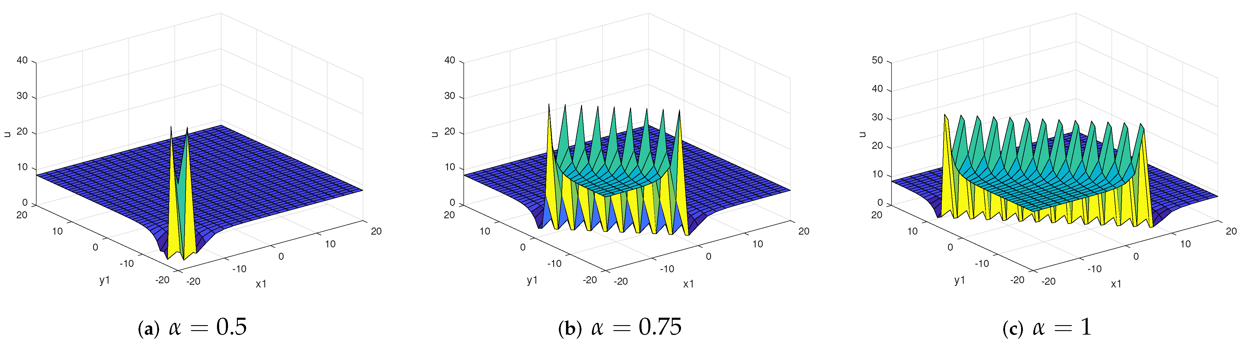
Taking solutions in Equation (53) as an example, we give the following images of the exact solutions. It is evident from Figure 1a–c that when the time changes slightly, both the amplitude and the shape of the waves vary markedly in the $x_1-y_1$ plane with fixed $x_2=y_2=9.7,\alpha =0.9$. In addition, it can be seen from Figure 2a–c that the exact solutions can be influenced by fractional-order $\alpha$ of the (4+1)-dimensional time-fractional Fokas equation. As $\alpha$ increases, the waveform becomes regular, the amplitude increases, and the wavelength becomes longer. Therefore, it can be inferred that the nonlinear phenomena of the (4+1)-dimensional time-fractional Fokas equations studied in this paper are very complex and changeable in practical problems. Additionally, the study of Equation (11) is very necessary and meaningful.

5. Numerical Solutions

In this section, the Gr$\ddot{u}$nwald–Letnikov method for the Riemann–Liouville time-fractional derivative and Fourier spectral method for spatial derivative are proposed to obtain the numerical solutions. Recently, Sun et al. numerically solved three-dimensional seismic waves; the spectral method was used for the numerical calculation in the spatial direction [35]. The method proposed by them is different from the traditional spectral method, where the difference mainly lies in the discrete calculation for each spatial direction, fast Fourier transform and inverse fast Fourier transform operations for each spatial direction, respectively. This saves a lot of calculations, and it is very beneficial to the numerical calculation for high-dimensional problems. This makes it easier for some high-dimensional problems to be solved numerically, without the difficulty of the numerical calculation due to the increase in dimension. Inspired by this, we apply it to the (4+1)-dimensional time-fractional equation that we study in this paper.

Considering the (4+1)-dimensional time-fractional Fokas equation as

$$\begin{array}{cc}\hfill & 16D_t^{\alpha }{u}_{x_2}-u_{x_1{x}_1{x}_1{x}_1}-u_{x_2{x}_2{x}_2{x}_2}+6u_{x_1{x}_1{x}_2{x}_2{x}_2}-12{\left(u^2\right)}_{x_2{x}_2}\hfill \\ & +12{\left(u^2\right)}_{x_1{x}_1}-24u_{y_1{y}_1}+24u_{y_2{y}_2}=0,(x_1,x_2,y_1,y_2)\in \mathrm{\Omega }\subset R^4,t\in (0,T],\hfill \end{array}$$

(56)

$$\begin{array}{cc}\hfill & u(x_1.x_2,y_1,y_2,0)=u_0(x_1,x_2,y_1,y_2),(x_1,x_2,y_1,y_2)\in \partial \mathrm{\Omega }\cup \mathrm{\Omega },\hfill \end{array}$$

(57)

$$\begin{array}{cc}\hfill & u(x_1.x_2,y_1,y_2,t)=\varphi (x_1,x_2,y_1,y_2,t),(x_1,x_2,y_1,y_2)\in \partial \mathrm{\Omega },t\in (0,T].\hfill \end{array}$$

(58)

5.1. Time Discretization

Take time-step $\tau =\frac{T}{N}$ with N as a positive integer and denote time points $t=n\tau (0\le n\le N)$. The grid function can be given as $p=\left\{p^n\right|0\le n\le N\}$. Using the Gr$\ddot{u}$nwald–Letnikov method for the Riemann–Liouville time-fractional derivative operator $D_t^{\alpha }$ leads to

$$\begin{array}{c}\hfill D_t^{\alpha }{p}^n\approx {\tau }^{-\alpha }\sum _{s=0}^n{w}_s^{\left(\alpha \right)}{p}^{n-s},\end{array}$$

(59)

where $w_s^{\left(\alpha \right)}={(-1)}^s\left(\genfrac{}{}{0pt}{}{\alpha }{s}\right)$, and $\left(\genfrac{}{}{0pt}{}{\alpha }{s}\right)=\frac{\mathrm{\Gamma }(\alpha +1)}{\mathrm{\Gamma }(s+1)\mathrm{\Gamma }(\alpha -s+1)}$.

5.2. Space Discretization

In space, we suppose the space domain $\mathrm{\Omega }=[0,a]\times [0,b]\times [0,c]\times [0,d]$ and spatial mesh size $h_1=\frac{a}{M_1},h_2=\frac{b}{M_2},h_3=\frac{c}{M_3},h_4=\frac{d}{M_4}$, where $h_1=h_2=h_3=h_4$, and $M_1,M_2,M_3,M_4$ are both integral powers of 2. The gird points can be given as $x_{1j}=j{h}_1(0\le j\le M_1)$, $x_{2k}=k{h}_2(0\le k\le M_2)$, $y_{1l}=l{h}_3(0\le l\le M_3)$, $y_{2m}=m{h}_4(0\le m\le M_4)$. Denote the index sets as

$$\begin{array}{cc}\hfill \hslash & =\left\{(j,k,l,m)\right|0<j<M_1,0<k<M_2,0<l<M_3,0<m<M_4\},\hfill \\ \hfill \ell & =\left\{(j,k,l,m)\right|0\le j\le M_1,0\le k\le M_2,0\le l\le M_3,0\le m\le M_4\},\hfill \\ \hfill \pounds & =\left\{j,k,l,m\right|j=0,orj=M_1;ork=0,ork=M_2;orl=0,orl=M_3;orm=0,orm=M_4\}.\hfill \end{array}$$

(60)

So each grid point can be represented by its coordinate $(j,k,l,m)$. The grid function can be given as $v=\left\{v_{jklm}\right|(j,k,l,m)\in \ell \}$.

5.3. The Numerical Scheme

Taking the $x_1$ direction as an example, the numerical method of the space directions is illustrated. Denoting $k_{x_1}=\frac{2\pi r_1}{a}$, where $r_1=-\frac{M_1}{2},-\frac{M_1}{2}+1,···,\frac{M_1}{2}-1$, and there are $M_1$ grid points in the $x_1$ direction when fixed $x_2,y_1,y_2$ and t.

Step 1: Take out the value of u at each grid node in the $x_1$ direction (there are $M_2*M_3*M_4$ columns in totals, one column has $M_1$ values) and take the fast Fourier transform for each column of data. We know that when $x_2,y_1,y_2$ and t are fixed, the $u(x_1,x_{2k},y_{1l},y_{2m},t_n)$ is a one-dimensional function of $x_1$. So the fast Fourier transform for $u(x_1,x_{2k},y_{1l},y_{2m},t_n)$ can be given as

$$\begin{array}{c}\hfill F_{x_1}\left[u_j\right]=\sum _{i=0}^{M_1-1}{u}_j{e}^{-i{k}_{x_1}{x}_{1j}},\end{array}$$

(61)

where $k_{x_1}=\frac{2\pi r_1}{a}$, $\frac{-M_1}{2}\le r_1\le \frac{M_1}{2}-1$.

When taking the fast Fourier transform of each column of data, the fast Fourier transform of $u(x_1,x_2,y_1,y_2,t)$ in the $x_1$ direction is completed, called $F_{x_1}\left[u\right]$.

Step 2: The derivative of the Fourier transform for $u(x_1,x_{2k},y_{1l},y_{2m},t_n)$ is as follows:

$$\begin{array}{c}\hfill F_{x_1}\left[{\left(u_{x_1{x}_1{x}_1{x}_1}\right)}_j\right]=k_{x_1}^4{F}_{x_1}\left[u_j\right],\end{array}$$

(62)

so, we have

$$\begin{array}{c}\hfill F_{x_1}\left[u_{x_1{x}_1{x}_1{x}_1}\right]=k_{x_1}^4{F}_{x_1}\left[u\right].\end{array}$$

(63)

Step 3: Inverse fast Fourier transform of $u(x_1,x_{2j},y_{1l},y_{2m},t_n)$ can be given as

$$\begin{array}{c}\hfill F_{x_1}^{-1}\left[u_j\right]=\frac{1}{M_1}\sum _{r_1=\frac{-M_1}{2}}^{\frac{M_1}{2}-1}{F}_{x_1}\left[u_j\right]e^{i{k}_{x_1}{x}_{1j}},0\le j\le M_1-1,\end{array}$$

(64)

where $k_{x_1}=\frac{2\pi r_1}{a}$, $\frac{-M_1}{2}\le r_1\le \frac{M_1}{2}-1$.

Similarly, when taking the inverse fast Fourier transform of each column of data, the inverse fast Fourier transform of $u(x_1,x_2,y_1,y_2,t)$ in the $x_1$ direction is completed, called $F_{x_1}^{-1}\left[u\right]$. So, for $u_{x_1{x}_1{x}_1{x}_1}(x_1,x_2,y_1,y_2,t)$, we have $u_{x_1{x}_1{x}_1{x}_1}=F_{x_1}^{-1}\left\{k_{x_1}^4{F}_{x_1}\left[u\right]\right\}$.

Similarly, we have

$$\begin{array}{cc}\hfill u_{x_2{x}_2{x}_2{x}_2}& =F_{x_2}^{-1}\left\{k_{x_2}^4{F}_{x_2}\left[u\right]\right\},u_{x_1{x}_1{x}_2{x}_2{x}_2}=F_{x_2}^{-1}\left\{i{k}_{x_2}^3{F}_{x_2}\left\{F_{x_1}^{-1}\{-k_{x_1}^2{F}_{x_1}\left[u\right]\}\right\}\right\},\hfill \\ \hfill {\left(u^2\right)}_{x_1{x}_1}& =F_{x_1}^{-1}\{-k_{x_1}^2{F}_{x_1}\left[{\left(u\right)}^2\right]\},{\left(u^2\right)}_{x_2{x}_2}=F_{x_2}^{-1}\{-k_{x_2}^2{F}_{x_2}\left[{\left(u\right)}^2\right]\},\hfill \\ \hfill u_{y_1{y}_1}& =F_{y_1}^{-1}\{-k_{y_1}^2{F}_{y_1}\left[u\right]\},u_{y_2{y}_2}=F_{y_2}^{-1}\{-k_{y_2}^2{F}_{y_2}\left[u\right]\},\hfill \end{array}$$

(65)

where $k_{x_2}=\frac{2\pi r_2}{b},k_{y_1}=\frac{2\pi r_3}{c},k_{y_2}=\frac{2\pi r_3}{d}$, $r_2=-\frac{M_2}{2},-\frac{M_2}{2}+1,···,\frac{M_2}{2}-1$, $r_3=-\frac{M_3}{2},-\frac{M_3}{2}+1,···,\frac{M_3}{2}-1$, $r_4=-\frac{M_4}{2},-\frac{M_4}{2}+1,···,\frac{M_4}{2}-1$. $F_{x_2}\left[u\right]$, $F_{y_1}\left[u\right]$ and $F_{y_2}\left[u\right]$ are Fast Fourier transform of $u(x_1,x_2,y_1,y_2,t)$ in $x_2$ direction, $y_1$ direction and $y_2$ direction, respectively.

Consider Equations (56)–(58) at the point $(x_{1j},x_{2k},y_{1l},y_{2m},t_n)$. Denote grid function $\{U_{jklm}^n=u(x_{1j},x_{2k},y_{1l},y_{2m},t_n)|(j,k,l,m)\in \ell ,0\le n\le N\}$, and taking $v=D_t^{\alpha }u$, $V_{jklm}^n=D_t^{\alpha }{U}_{jklm}^n$, ${\left(V_{x_2}\right)}_{jklm}^n=D_t^{\alpha }{\left(U_{x_2}\right)}_{jklm}^n$, we have

$$\begin{array}{cc}\hfill 16{\left(V_{x_2}\right)}_{jklm}^n& =F_{x_1}^{-1}\left\{k_{x_1}^4{F}_{x_1}\left[U_{jklm}^n\right]\right\}+F_{x_2}^{-1}\left\{k_{x_2}^4{F}_{x_2}\left[U_{jklm}^n\right]\right\}\hfill \\ & -6F_{x_2}^{-1}\left\{i{k}_{x_2}^3{F}_{x_2}\left\{F_{x_1}^{-1}\{-k_{x_1}^2{F}_{x_1}\left[U_{jklm}^n\right]\}\right\}\right\}\hfill \\ & +12F_{x_2}^{-1}\{-k_{x_2}^2{F}_{x_2}\left[{\left(U_{jklm}^n\right)}^2\right]\}-12F_{x_1}^{-1}\{-k_{x_1}^2{F}_{x_1}\left[{\left(U_{jklm}^n\right)}^2\right]\}\hfill \\ & +24F_{y_1}^{-1}\{-k_{y_1}^2{F}_{y_1}\left[U_{jklm}^n\right]\}-24F_{y_2}^{-1}\{-k_{y_2}^2{F}_{y_2}\left[U_{jklm}^n\right]\},\hfill \\ & (j,k,l,m)\in \hslash ,1\le n\le N,\hfill \end{array}$$

(66)

$$\begin{array}{cc}\hfill U_{jklm}^0& =u_0(x_{1j},x_{2k},y_{1l},y_{2m}),(j,k,l,m)\in \ell ,\hfill \end{array}$$

(67)

$$\begin{array}{c}\\ \hfill U_{jklm}^n& =\varphi (x_{1j},x_{2k},y_{1l},y_{2m},t_n),(j,k,l,m)\in \pounds ,0\le n\le N.\hfill \end{array}$$

(68)

For the sake of simplicity, we have

$$\begin{array}{cc}\hfill A^n& =F_{x_1}^{-1}\left\{k_{x_1}^4{F}_{x_1}\left[U_{jklm}^n\right]\right\}+F_{x_2}^{-1}\left\{k_{x_2}^4{F}_{x_2}\left[U_{jklm}^n\right]\right\}\hfill \\ & -6F_{x_2}^{-1}\left\{i{k}_{x_2}^3{F}_{x_2}\left\{F_{x_1}^{-1}\{-k_{x_1}^2{F}_{x_1}\left[U_{jklm}^n\right]\}\right\}\right\}\hfill \\ & +12F_{x_2}^{-1}\{-k_{x_2}^2{F}_{x_2}\left[{\left(U_{jklm}^n\right)}^2\right]\}-12F_{x_1}^{-1}\{-k_{x_1}^2{F}_{x_1}\left[{\left(U_{jklm}^n\right)}^2\right]\}\hfill \\ & +24F_{y_1}^{-1}\{-k_{y_1}^2{F}_{y_1}\left[U_{jklm}^n\right]\}-24F_{y_2}^{-1}\{-k_{y_2}^2{F}_{y_2}\left[U_{jklm}^n\right]\},\hfill \\ & (j,k,l,m)\in \hslash ,1\le n\le N.\hfill \end{array}$$

(69)

So

$$\begin{array}{cc}\hfill 16{\left(V_{x_2}\right)}_{jklm}^n& =A^n,(j,k,l,m)\in \hslash ,1\le n\le N,\hfill \end{array}$$

(70)

$$\begin{array}{cc}\hfill U_{jklm}^0& =u_0(x_{1j},x_{2k},y_{1l},y_{2m}),(j,k,l,m)\in \ell ,\hfill \end{array}$$

(71)

$$\begin{array}{cc}\hfill U_{jklm}^n& =\varphi (x_{1j},x_{2k},y_{1l},y_{2m},t_n),(j,k,l,m)\in \pounds ,0\le n\le N.\hfill \end{array}$$

(72)

Taking the Fast Fourier transform and the Inverse Fourier transform both sides of Equation (70) with respect to the $x_2$ direction leads to

$$\begin{array}{cc}\hfill -16i{k}_{x_2}{F}_{x_2}\left[V_{jklm}^n\right]& =F_{x_2}\left[A^n\right],(j,k,l,m)\in \hslash ,1\le n\le N,\hfill \end{array}$$

(73)

$$\begin{array}{cc}\hfill V_{jklm}^n& =F_{x_2}^{-1}\left\{\frac{F_{x_2}\left[A^n\right]}{-16i{k}_{x_2}}\right\},(j,k,l,m)\in \hslash ,1\le n\le N,\hfill \end{array}$$

(74)

$$\begin{array}{cc}\hfill U_{jklm}^n& \approx \left({\tau }^{\alpha }{V}_{jklm}^n-\sum _{s=1}^n{w}_s^{\left(\alpha \right)}{U}_{jklm}^{n-s}\right)/w_0^{\left(\alpha \right)},(j,k,l,m)\in \hslash ,1\le n\le N,\hfill \end{array}$$

(75)

$$\begin{array}{cc}\hfill U_{jklm}^0& =u_0(x_{1j},x_{2k},y_{1l},y_{2m}),(j,k,l,m)\in \ell ,\hfill \end{array}$$

(76)

$$\begin{array}{cc}\hfill U_{jklm}^n& =\varphi (x_{1j},x_{2k},y_{1l},y_{2m},t_n),j=0,(j,k,l,m)\in \pounds ,0\le n\le N.\hfill \end{array}$$

(77)

Replacing $U_{jklm}^n$ with $u_{jklm}^n$ and replacing $V_{jklm}^n$ with $v_{jklm}^n$, we have

$$\begin{array}{cc}\hfill -16i{k}_{x_2}{F}_{x_2}\left[v_{jklm}^n\right]& =F_{x_2}\left[A^n\right],(j,k,l,m)\in \hslash ,1\le n\le N,\hfill \end{array}$$

(78)

$$\begin{array}{cc}\hfill v_{jklm}^n& =F_{x_2}^{-1}\left\{\frac{F_{x_2}\left[A^n\right]}{-16i{k}_{x_2}}\right\},(j,k,l,m)\in \hslash ,1\le n\le N,\hfill \end{array}$$

(79)

$$\begin{array}{cc}\hfill u_{jklm}^n& =\left({\tau }^{\alpha }{v}_{jklm}^n-\sum _{s=1}^n{w}_s^{\left(\alpha \right)}{u}_{jklm}^{n-s}\right)/w_0^{\left(\alpha \right)},(j,k,l,m)\in \hslash ,1\le n\le N,\hfill \end{array}$$

(80)

$$\begin{array}{cc}\hfill u_{jklm}^0& =u_0(x_{1j},x_{2k},y_{1l},y_{2m}),(j,k,l,m)\in \ell ,\hfill \end{array}$$

(81)

$$\begin{array}{cc}\hfill u_{jklm}^n& =\varphi (x_{1j},x_{2k},y_{1l},y_{2m},t_n),(j,k,l,m)\in \pounds ,0\le n\le N.\hfill \end{array}$$

(82)

5.4. Numerical Results

Periodic boundary conditions need to be considered when using the Fourier spectral method. In order to satisfy the periodic boundary condition, we consider the following two examples to illustrate the effectiveness of our numerical method proposed in Section 5.3.

Example 1.

An unbounded (4+1)-dimensional time-fractional Fokas equation based on Equation (11) can be described as follows:

$$\begin{array}{cc}\hfill & 16D_t^{\alpha }{u}_{x_2}-u_{x_1{x}_1{x}_1{x}_1}-u_{x_2{x}_2{x}_2{x}_2}+6u_{x_1{x}_1{x}_2{x}_2{x}_2}-12{\left(u^2\right)}_{x_2{x}_2}\hfill \\ & +12{\left(u^2\right)}_{x_1{x}_1}-24u_{y_1{y}_1}+24u_{y_2{y}_2}=f(x_1,x_2,y_1,y_2,t),\hfill \end{array}$$

(83)

where$(x_1,x_2,y_1,y_2)\in R^4,t\in (0,T]$and the exact solution of Equation (83) is

$$\begin{array}{c}\hfill u(x_1,x_2,y_1,y_2,t)=sec{h}^2\left(x_1+x_2+y_1+y_2+\frac{2t^{\alpha }}{\mathrm{\Gamma }(1+\alpha )}-6\right),\end{array}$$

(84)

where$\mathrm{\Gamma }\left(x\right)$is gamma function.

The initial condition, the boundary conditions and $f(x_1,x_2,y_1,y_2,t)$ are determined by exact solutions in Equation (84). In order to illustrate the validity of the numerical method proposed above, we compare the numerical solutions with the exact solutions in Equation (84). When $\alpha =0.75$, $\alpha =0.8$, $\alpha =0.9$ and $\alpha =1$, the maximum absolute errors of the time-fractional (4+1)-dimensional partial differential Fokas equation are shown in

Table 1. The maximum absolute errors between the numerical solutions and the exact solutions in Equation (84) for different fractional order $\alpha$.

$\mathit{\alpha }$	Errors	$\mathit{\alpha }$	Errors
0.75	5.8927 × ${10}^{-5}$	0.9	3.1545 × ${10}^{-5}$
0.8	5.2142 × ${10}^{-5}$	1	8.6031 × ${10}^{-11}$

. It can be seen from the table that the numerical results given by the Fourier spectral method and Gr$\ddot{u}$nwald–Letnikov method are satisfactory, which also shows the validity of this numerical method. In addition, some images of the comparison between numerical solutions and exact solutions for different fractional order $\alpha$ are given: $\alpha =0.75$ in Figure 3a, $\alpha =0.8$ in Figure 3b, $\alpha =0.9$ in Figure 3c, and $\alpha =1$ in Figure 3d. From these images, we can see that as $\alpha$ increases, the curves of the exact solutions and numerical solutions become closer. Additionally, the curve of the numerical solutions and the curve of the exact solutions are almost coincident with $\alpha =1$.

Example 2.

A bounded periodic (4+1)-dimensional time-fractional Fokas equation based on Equation (11) can be given as

$$\begin{array}{cc}\hfill & 16D_t^{\alpha }{u}_{x_2}-u_{x_1{x}_1{x}_1{x}_1}-u_{x_2{x}_2{x}_2{x}_2}+6u_{x_1{x}_1{x}_2{x}_2{x}_2}-12{\left(u^2\right)}_{x_2{x}_2}\hfill \\ & +12{\left(u^2\right)}_{x_1{x}_1}-24u_{y_1{y}_1}+24u_{y_2{y}_2}=g(x_1,x_2,y_1,y_2,t),\hfill \end{array}$$

(85)

where$(x_1,x_2,y_1,y_2)\in [0,2\pi ]\times [0,2\pi ]\times [0,2\pi ]\times [0,2\pi ],t\in (0,t]$and the exact solution of Equation (85) is

$$\begin{array}{c}\hfill u(x_1,x_2,y_1,y_2,t)=e^{-\frac{t^{\alpha }}{\mathrm{\Gamma }(1+\alpha )}}sin(x_1+x_2+y_1+y_2),\end{array}$$

(86)

where$\mathrm{\Gamma }\left(x\right)$is gamma function.

The initial condition, the boundary conditions and $g(x_1,x_2,y_1,y_2,t)$ are determined by exact solutions in Equation (86). As in Example 1, for different fractional order $\alpha$, the maximum absolute errors between the numerical solutions and the exact solutions in Equation (86) are given in

Table 2. The maximum absolute errors between the numerical solutions and the exact solutions in Equation (86) for different fractional order $\alpha$.

$\mathit{\alpha }$	Errors	$\mathit{\alpha }$	Errors
0.75	1.5015 × ${10}^{-5}$	0.9	1.6518 × ${10}^{-8}$
0.8	1.3549 × ${10}^{-7}$	1	2.0000 × ${10}^{-9}$

, and the comparison images between the numerical solutions and exact solutions in Equation (86) are given in Figure 4. We can see from the table that the error results under different fractional order $\alpha$ are acceptable, and it is obvious that the curve-fitting results in the figure are satisfactory. The feasibility of the proposed numerical method can be also judged from the error results and curve-fitting results.

6. Conclusions

In this paper, we studied an uncommon Fokas equation. The (4+1)-dimensional time-fractional Fokas equation in the sense of the Riemann–Liouville fractional derivative was derived in detail for the first time. For the (4+1)-dimensional time-fractional Fokas equation, the Lie symmetry analysis method was used to investigate the symmetry of the equation, and at the same time, we discussed the conservational laws of the equation. In addition, several exact traveling wave solutions were obtained by using the $\left(\frac{G^{\prime }}{G}\right)$-expansion method, and numerical solutions were obtained by using the Fourier spectral method and the Gr$\ddot{u}$nwald–Letnikov method. The error results between numerical solutions and exact solutions showed the effectiveness of the numerical method considered in this paper, and the numerical method may be helpful for the study of this kind of high-dimensional problem.

References

- He, Y. Exact Solutions for (4+1)-Dimensional Nonlinear Fokas Equation Using Extended F-Expansion Method and Its Variant. Math. Probl. Eng. 2014, 2014, 4–17. [Google Scholar]
- Fan, L.L.; Bao, T. Lumps and interaction solutions to the (4+1)-dimensional variable-coefficient Kadomtsev-Petviashvili equation in fluid mechanics. Int. J. Mod. Phys. B 2021, 35, 2150223. [Google Scholar] [CrossRef]
- Han, P.F.; Bao, T. Integrability aspects and some abundant solutions for a new (4 + 1)-dimensional KdV-like equation. Int. J. Mod. Phys. B 2021, 35, 2150079. [Google Scholar] [CrossRef]
- Bagley, R.L.; Torvik, P.J. A theoretical basis for the application of fractional calculus. J. Rheol. 1983, 27, 201–210. [Google Scholar] [CrossRef]
- Lakshmikantham, V.; Vatsala, A.S. Basic theory of fractional differential equations. Nonlinear Anal. 2008, 69, 2677–2682. [Google Scholar] [CrossRef]
- Glockle, W.G.; Nonnenmacher, T.F. A fractional calculus approach to self similar protein dynamics. Biophys. J. 1995, 68, 46–53. [Google Scholar] [CrossRef] [Green Version]
- Fokas, A.S. Integrable nonlinear evolution partial differential equations in 4 + 2 and 3 + 1 dimensions. Phys. Rev. Lett. 2006, 96, 190210. [Google Scholar] [CrossRef]
- Singla, K.; Gupta, R.K. On invariant analysis of some time fractional nonlinear systems of partial differential equations. J. Math. Phys. 2016, 57, 1309–1322. [Google Scholar] [CrossRef]
- Biswas, A.; Khalique, C.M. Stationary solutions for nonlinear dispersive Schrödinger’s equation. Nonlinear Dyn. 2010, 63, 623–626. [Google Scholar] [CrossRef]
- Krishnan, E.V.; Kumar, S.; Biswas, A. Solitons and other nonlinear waves of the Boussinesq equation. Nonlinear Dyn. 2015, 70, 1213–1221. [Google Scholar] [CrossRef]
- Noether, E. Invariante variationsprobleme. Transp. Theory. Stat. Phys. 1971, 1, 186–207. [Google Scholar] [CrossRef] [Green Version]
- Atanackovic, T.M.; Konjik, S.; Pilipovic, S.; Simic, S. Variational problems with fractional derivative. Nonlinear Anal. 2009, 71, 1504–1517. [Google Scholar] [CrossRef] [Green Version]
- Malinowska, A.B. A formulation of the fractional Noether-type theorem for multidimensional lagrangians. Appl. Math. Lett. 2012, 25, 1941–1946. [Google Scholar] [CrossRef] [Green Version]
- Odzijewicz, T.; Malinowska, A.B.; Torres, D.F.M. Neother’s theorem for fractional variational problems of variable order. Cent. Eur. J. Phys. 2013, 11, 691–701. [Google Scholar]
- Ibragimov, N.H. A new conservation theorem. J. Math. Anal. Appl. 2007, 333, 311–328. [Google Scholar] [CrossRef] [Green Version]
- Lukashchuk, S.Y. Conservation laws for time-fractional subdiffusion and diffusion-wave equations. Nonlinear Dyn. 2015, 80, 791–802. [Google Scholar] [CrossRef] [Green Version]
- Lee, J.; Sakthivel, R.; Wazzan, L. Exact traveling wave solutions of a higher-dimensional nonlinear evolution equation. Mod. Phys. Lett. B 2010, 24, 1011–1021. [Google Scholar] [CrossRef]
- Kim, H.; Sakthivel, R. New exact traveling wave solutions of some nonlinear higher-dimensional physical models. Rep. Math. Phys. 2012, 70, 39–50. [Google Scholar] [CrossRef]
- Zhang, S.; Chen, M. Painlevé integrability and new exact solutions of the (4+1)-dimensional Fokas equation. Math. Probl. Eng. 2015, 2015, 1–7. [Google Scholar] [CrossRef] [Green Version]
- Al-Amr, M.O.; El-Ganaini, S. New exact traveling wave solutions of the (4+1)-dimensional Fokas equation. Comput. Math. Appl. 2017, 74, 1274–1287. [Google Scholar] [CrossRef]
- Wang, X.B.; Tian, S.F.; Feng, L.L.; Zhang, T.T. On quasi-periodic waves and rogue waves to the (4+1)-dimensional nonlinear Fokas equation. J. Math. Phys. 2018, 59, 073505. [Google Scholar] [CrossRef]
- Cao, Y.; He, J.; Cheng, Y.; Mihalache, D. Reductions of the (4+1)-dimensional Fokas equation and their solutions. Nonlinear Dyn. 2020, 99, 3013–3028. [Google Scholar] [CrossRef]
- Kumar, S.; Kumar, D.; Kumar, A. Lie symmetry analysis for obtaining the abundant exact solutions, optimal system and dynamics of solitons for a higher-dimensional Fokas equation. Chaos Soliton Fractals 2021, 142, 110507. [Google Scholar] [CrossRef]
- Wang, M.L.; Li, X.Z.; Zhang, J.L. The (G′/G)-expansion method and travelling wave solutions of nonlinear evolution equations in mathematical physics. Phys. Lett. A 2008, 372, 417–423. [Google Scholar] [CrossRef]
- Bekir, A. Application of the (G′/G)-expansion method for nonlinear evolution equations. Phys. Lett. A 2008, 372, 3400–3406. [Google Scholar] [CrossRef]
- Zhang, S.; Tong, J.L.; Wang, W. A generalized (G′/G)-expansion method for the mKdV equation with variable coeffificients. Phys. Lett. A 2008, 372, 2254–2257. [Google Scholar] [CrossRef]
- Kim, H.; Sakthivel, R. Travelling wave solutions for time-delayed nonlinear evolution equations. Appl. Math. Lett. 2010, 23, 527–532. [Google Scholar] [CrossRef] [Green Version]
- Akbar, M.A.; Ali, N.H.M. The alternative (G′/G)-expansion method and its applications to nonlinear partial differential equations. Int. J. Phys. Sci. 2011, 6, 7910–7920. [Google Scholar]
- Akbar, M.; Ali, N.; Zayed, E. The generalized and improved (G′/G)-expansion method combined with the Jacobi elliptic equation. Commun Theor Phys. 2014, 61, 669–676. [Google Scholar] [CrossRef]
- Miah, M.; Ali, H.; Akbar, M.; Seadawy, A. New applications of the two varibable (G′/G,1/G)-expansion method for closed form traveling wave solutions of integro-differential equations. J. Ocean Eng. Sci. 2019, 4, 132–143. [Google Scholar] [CrossRef]
- Bi, S.Y.; Hou, C.M.; Jin, Y.; Wang, J.; Ji, S. An Alternating Direction Difference Scheme for Solving Four Dimension Reaction Diffusion Equation with Constant Coefficients. Adv. Sci. Tech. Lett. 2016, 139, 202–207. [Google Scholar]
- Ma, H.J.; Wang, Y. Full Information H2 Control of Borel-Measurable Markov Jump Systems with Multiplicative Noises. Mathematics 2021, 10, 37. [Google Scholar] [CrossRef]
- Chaljub, E.; Capdeville, Y.; Vilotte, J.P. Solving elastodynamics in a fluid-solid heterogeneous sphere: A parallel spectral element approximation on non-conforming grids. J. Comp. Phys. 2003, 187, 457–491. [Google Scholar] [CrossRef]
- Furumura, T.; Kennett, B.L.N.; Takenaka, H. Parallel 3-D pseudospectral simulation of seismic wave propagation. Geophysics 1998, 63, 279–288. [Google Scholar] [CrossRef]
- Sun, X.G.; Zhang, D. A comparative study of finite difference method and pseudo-spectral method in seismic wave simulation. Chin. Sci. Tech. Papers. 2018, 13, 2005–2008. (In Chinese) [Google Scholar]
- Wang, J. Numerical simulation of three-dimensional seismic wave field and its application. Coal Chem. Ind. 2020, 43, 46–50. (In Chinese) [Google Scholar]
- Wu, Y.; Zhao, X.Y.; Guo, Z.Q.; Feng, X.; Lu, Q. Numerical dispersion analysis of the pseudo-spectral algorithm in the numerical simulation of acoustic waves. Earthquake 2017, 37, 135–146. (In Chinese) [Google Scholar]
- Wang, G.W.; Liu, X.Q.; Zhang, Y.Y. Lie symmetry analysis to the time fractional generalized fifth order KdV equation. Commun. Nonlinear Sci. Numer. Simul. 2013, 18, 2321–2326. [Google Scholar] [CrossRef]
- Elboree, M.K. Conservation laws, soliton solutions for modified Camassa-Holm equaion and (2+1)-dimensional ZK-BBM equation. Nonlinear Dyn. 2017, 89, 1–16. [Google Scholar] [CrossRef]
- Sahoo, S.; Ray, S.S. Analysis of Lie symmetries with conservation laws for the (3+1) dimensional time-fractional mKdV-ZK equation in ionacoustic waves. Nonlinear Dyn. 2017, 90, 1105–1113. [Google Scholar] [CrossRef]
- Chatibi, Y.; El Kinani, E.H.; Ouhadan, A. Lie symmetry analysis and conservation laws for the time fractional Black-Scholes equation. Int. J. Geom. Methods Mod. Phys. 2020, 17, 2050010. [Google Scholar] [CrossRef]
- Yaıar, E.; Yıldırım, Y.; Khalique, C.M. Lie symmetry analysis, conservation laws and exact solutions of the seventh-order time fractional Sawada-Kotera-Ito equation. Results Phys. 2016, 6, 322–328. [Google Scholar] [CrossRef] [Green Version]
- Feng, L.L.; Tian, S.F.; Wang, X.B.; Zhang, T.T. Lie symmetry analysis, conservation laws and exact power series solutions for time-fractional Fordy-Gibbons equation. Commun. Theor. Phys. 2016, 66, 321–329. [Google Scholar] [CrossRef]
- Rui, W.; Zhang, X. Lie symmetries and conservation laws for the time fractional Derrida-Lebowitz-Speer-Spohn equation. Commun. Nonlinear Sci. Numer. Simul. 2016, 34, 38–44. [Google Scholar] [CrossRef]
- Zahra, W.K.; Van Daele, M. Discrete spline methods for solving two point fractional Bagley-Torvik equation. Appl. Math. Comput. 2017, 296, 42–56. [Google Scholar] [CrossRef]
- Wang, Y.; Yan, Y.; Yan, Y.; Pani, A.K. Higher order time stepping methods for subdiffusion problems based on weighted and shifted Grünwald-Letnikov formulae with nonsmooth data. J. Sci. Comput. 2020, 83, 1–29. [Google Scholar] [CrossRef]
- Gazizov, R.K.; Kasatkin, A.A.; Lukashchuk, S. Continuous transformation groups of fractional differential equations. Vestnik. USATU 2007, 9, 125–135. [Google Scholar]
- Sahadevan, R.; Bakkyaraj, T. Invariant analysis of time fractional generalized Burgers and Korteweg-de Vries equations. J. Math. Anal. Appl. 2012, 393, 341–347. [Google Scholar] [CrossRef] [Green Version]
- Agrawal, O.P. Formulation of euler-lagrange equations for fractional variational problems. J. Math. Anal. Appl. 2002, 272, 368–379. [Google Scholar] [CrossRef] [Green Version]
Figure 1.
Exact solutions in Equation (53) at different time with , , , , , , , , , , , , .
Figure 2.
Exact solutions in Equation (53) for different with , , , , , , , , , , , , .
Figure 3.
Example 1. Comparison of the numerical solutions and the exact solutions in Equation (84) at the end time for different fractional order with .
Figure 4.
Example 2. Comparison of the numerical solutions and the exact solutions in Equation (86) at the end time for different fractional order with .