
Particle Swarm Optimization Fractional Slope Entropy: A New Time Series Complexity Indicator for Bearing Fault Diagnosis


Abstract
:1. Introduction
2. Algorithms
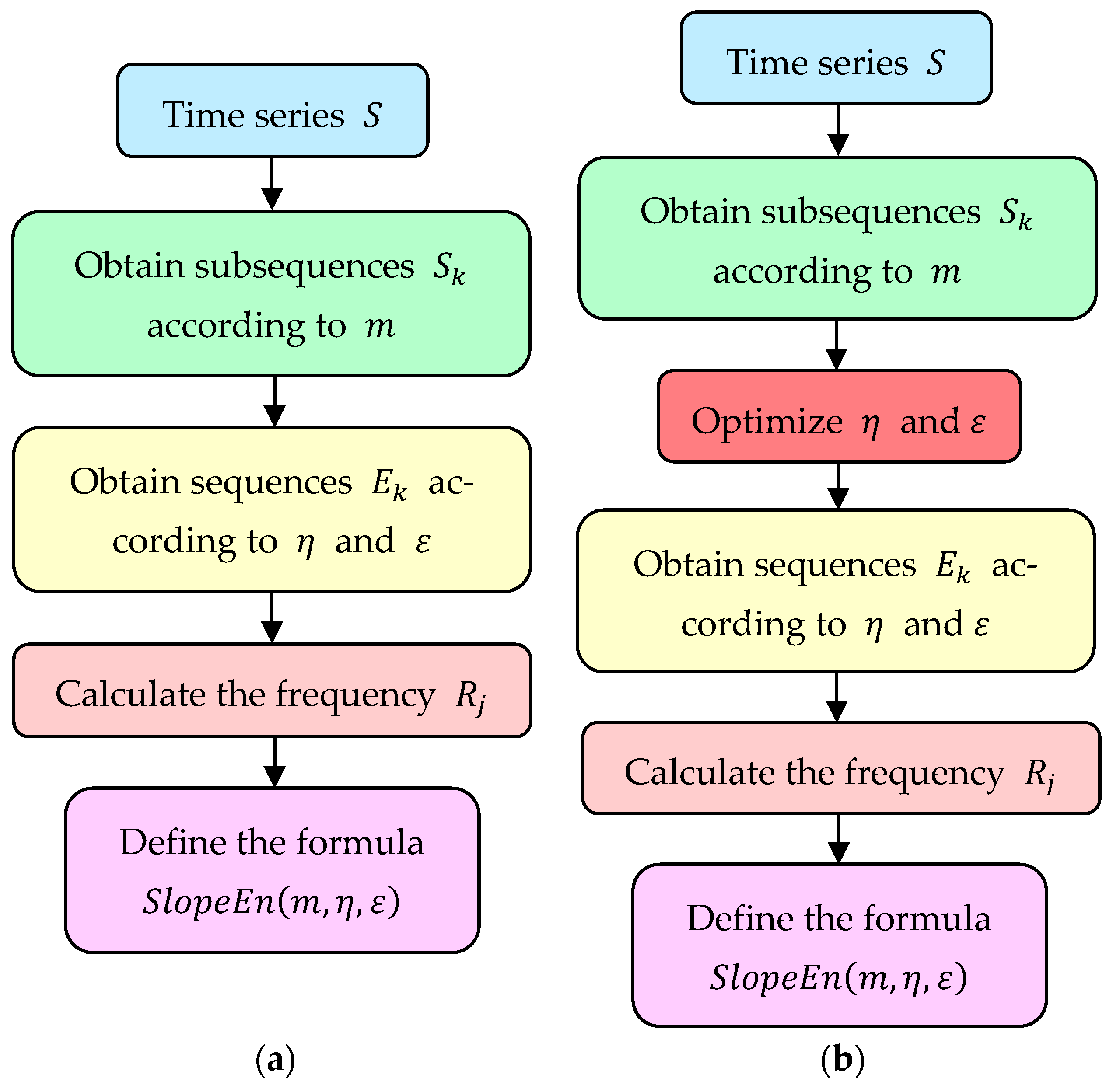
2.1. Slope Entropy Algorithm
- Step 1:
- set an embedding dimension m, which can divide the time series into subsequences, where m is greater than two and much less than . The disintegrate form is as follows:
- Step 2:
- subtract the latter of the two adjacent elements in all the subsequences obtained in Step 1 from the former to obtain k new sequences. The new form is as follows:
- Step 3:
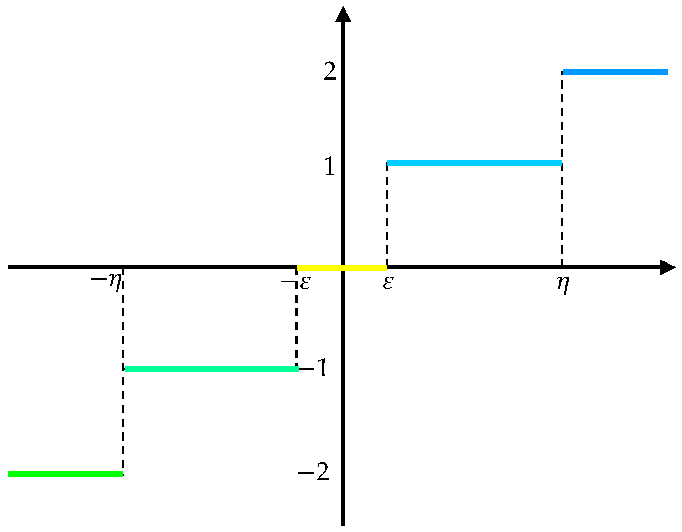
- lead into the two threshold parameters and of SlEn, where , and compare all elements in the sequences obtained from Step 2 with the positive and negative values of these two threshold parameters. The positive and negative values of these two threshold parameters and serve as the dividing lines, they divide the number field into five modules , and . If , the module is ; if , the module is ; if , the module is ; if , the module is ; if , the module is ; if , the module is . The intuitive module division principle is shown by the coordinate axis in Figure 1 below:
- Step 4:
- the number of modules is 5, so all types of the sequences are counted as . Such as when m is 3, there will be at most 25 types of , which are , , …, , , …, , . The number of each type records as , and the frequency of each type is calculated as follows:
- Step 5:
- based on the classical Shannon entropy, the formula of SlEn is defined as follows:
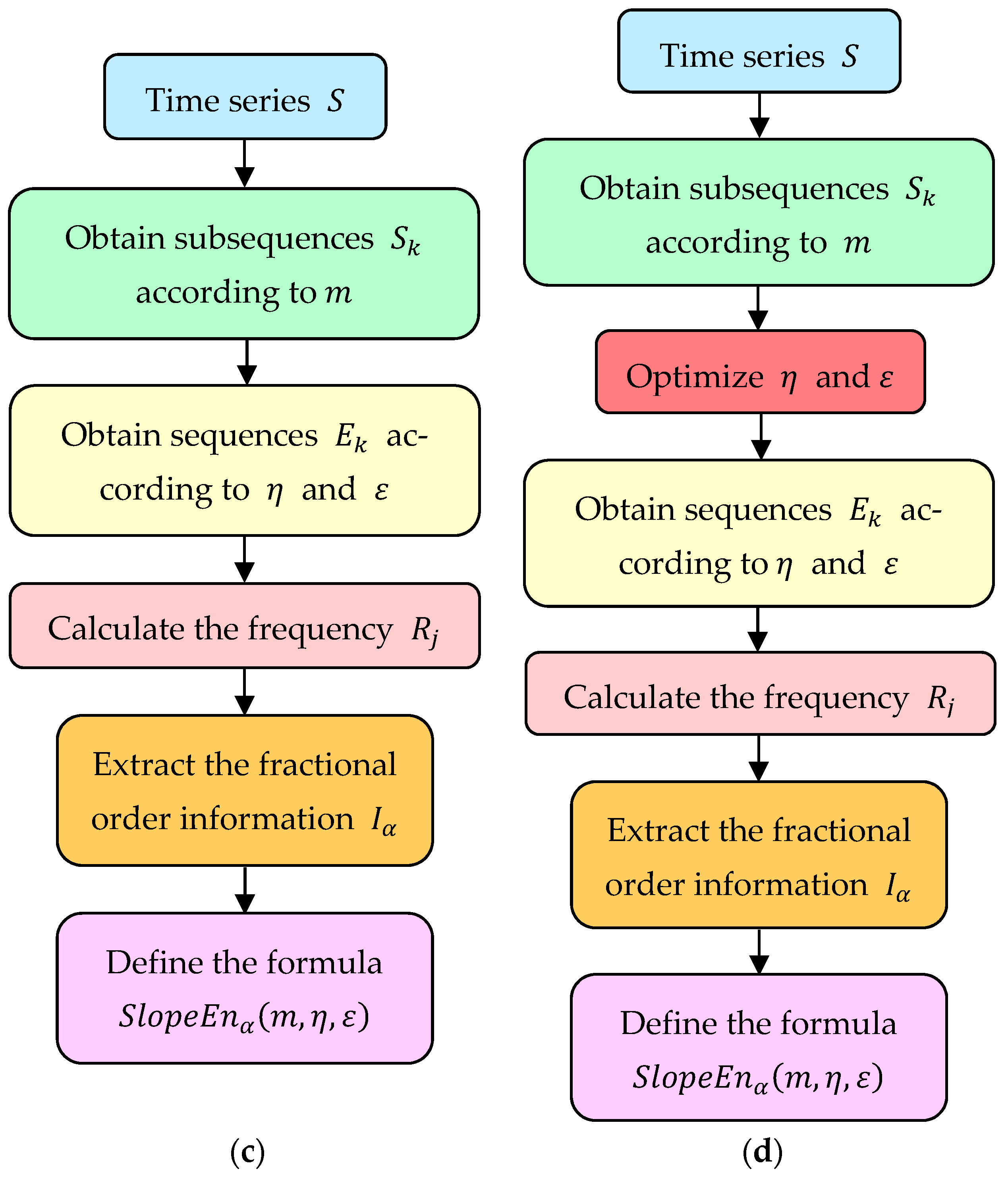
2.2. Fractional Slope Entropy Algorithm
- Step 1:
- Shannon entropy is the first entropy to consider fractional calculus, and its generalized expression is as follows:
- Step 2:
- extract the fractional order information of order from Equation (6):
- Step 3:
- combine the fractional order with SlEn, which is to replace with Equation (7). Therefore, the formula of FrSlEn is defined as follows:
2.3. Particle Swarm Optimization and Algorithm Process
3. Proposed Feature Extraction Methods
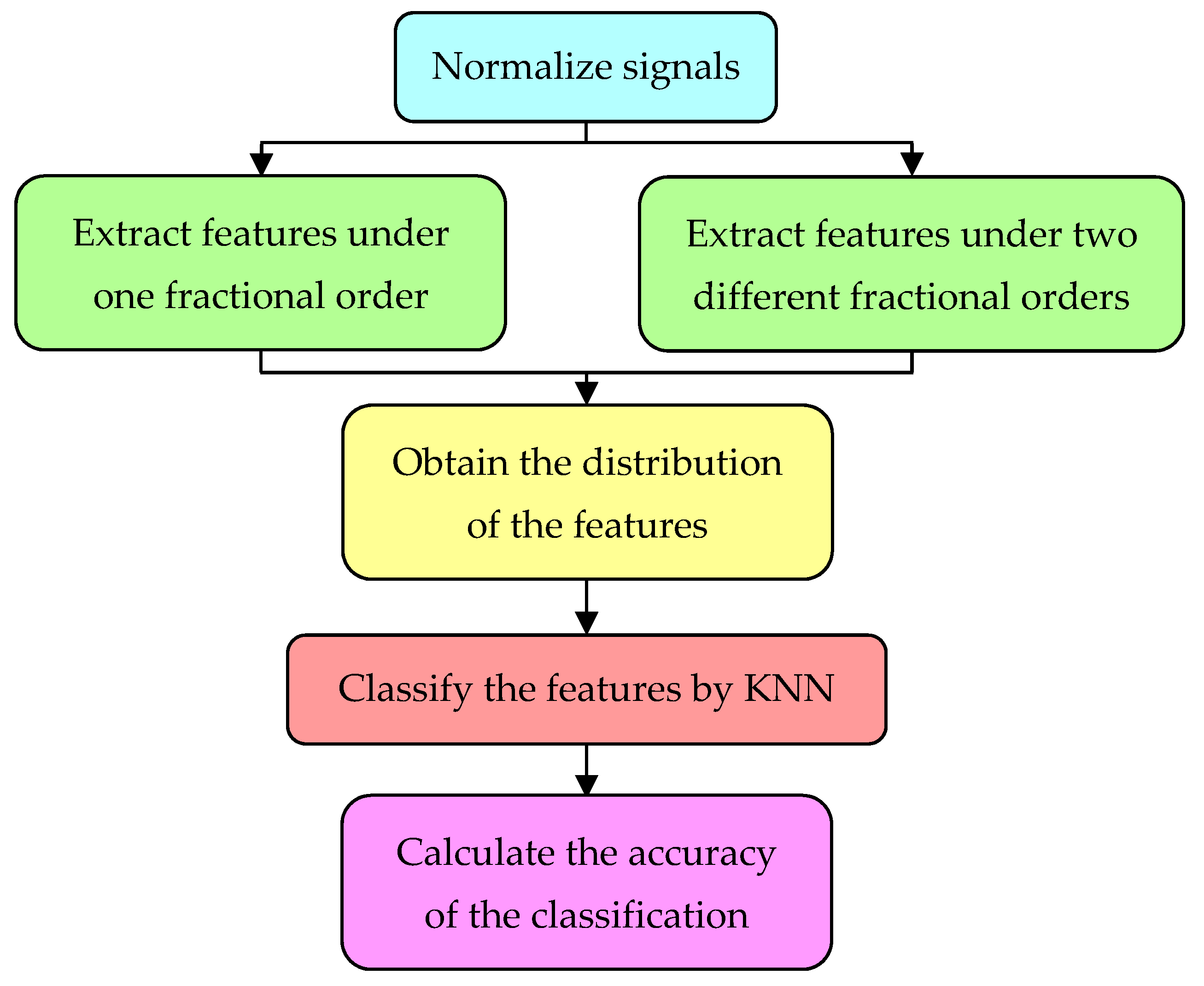
- Step 1:
- the 10 kinds of bearing signals are normalized, which can make the signals neat and regular, the threshold parameters and less than 1, where is less than 0.2 in most cases.
- Step 2:
- the five kinds of single features of these 10 kinds of normalized bearing signals are extracted separately under seven different fractional orders.
- Step 3:
- the distribution of the features is obtained and the hybrid degrees between the feature points are observed.
- Step 4:
- these features are classified into one of the 10 bearing signals by K-Nearest Neighbor (KNN).
- Step 5:
- the classification accuracies of the features are calculated.
4. Single Feature Extraction
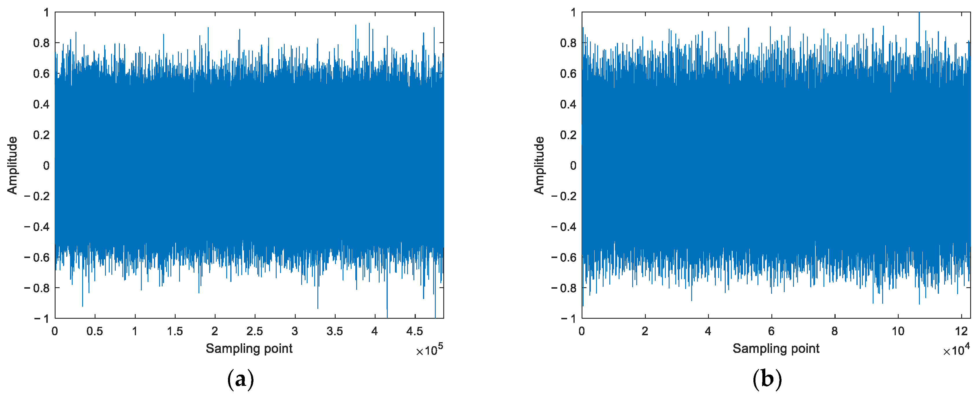
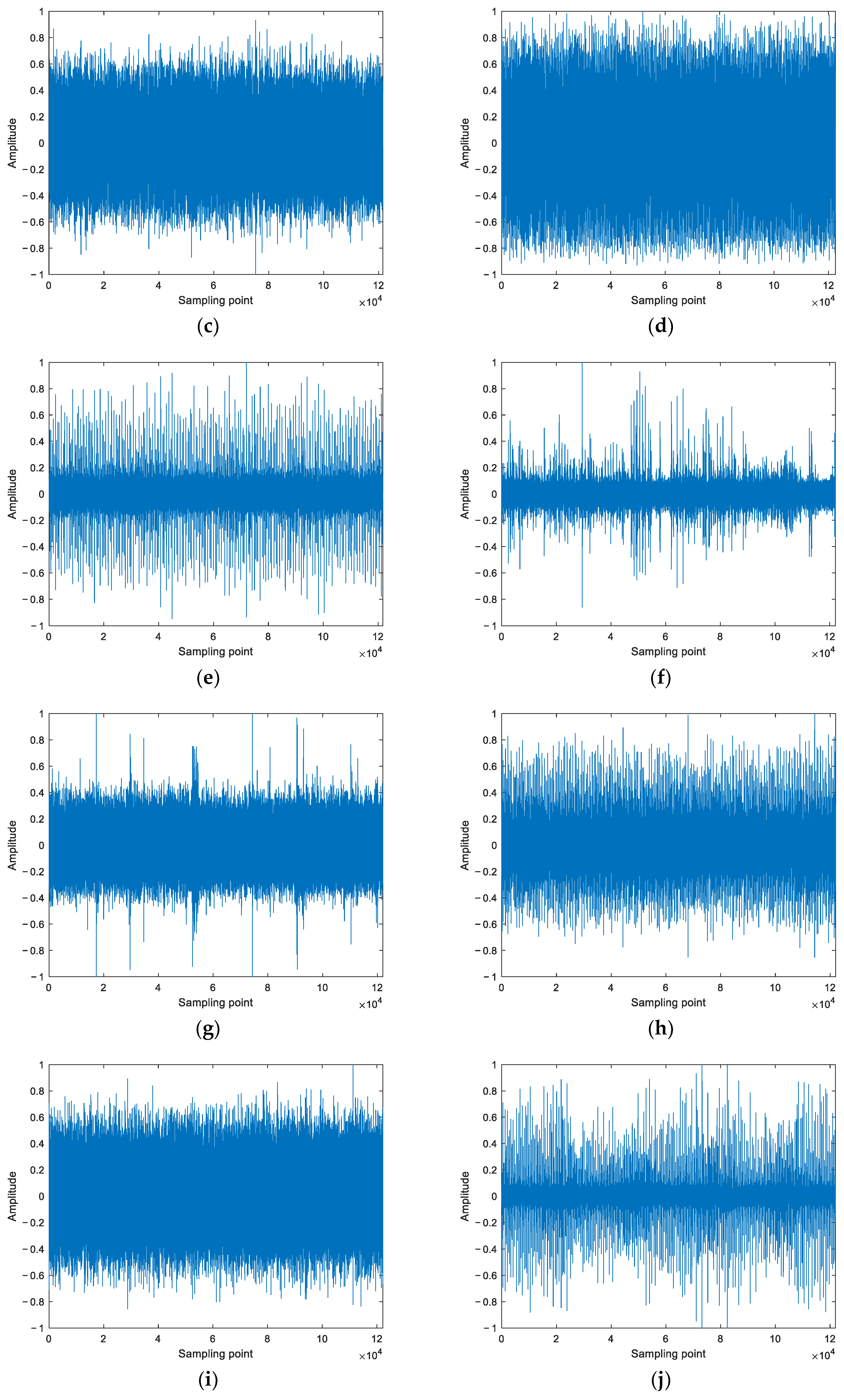
4.1. Bearing Signals
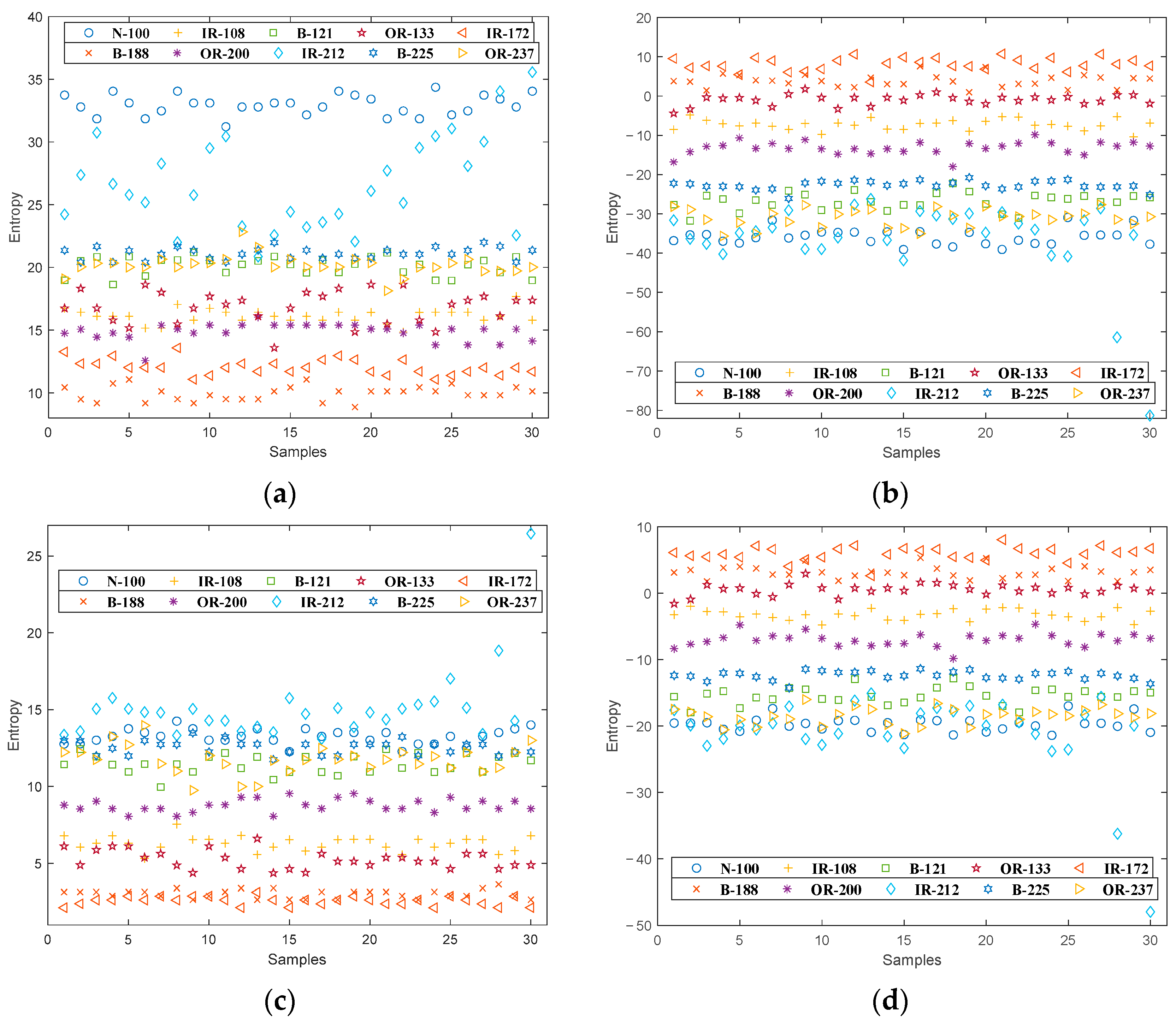
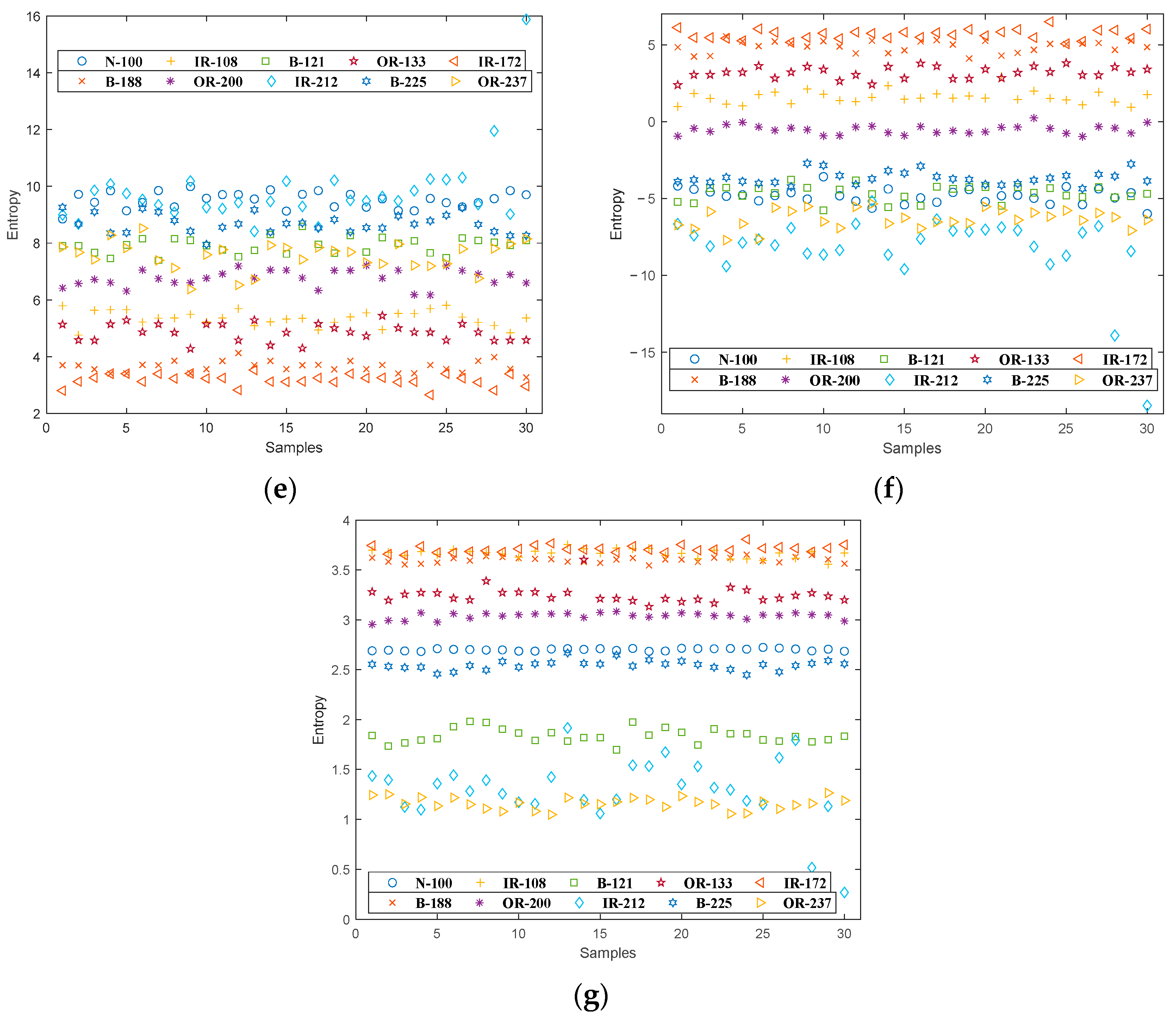
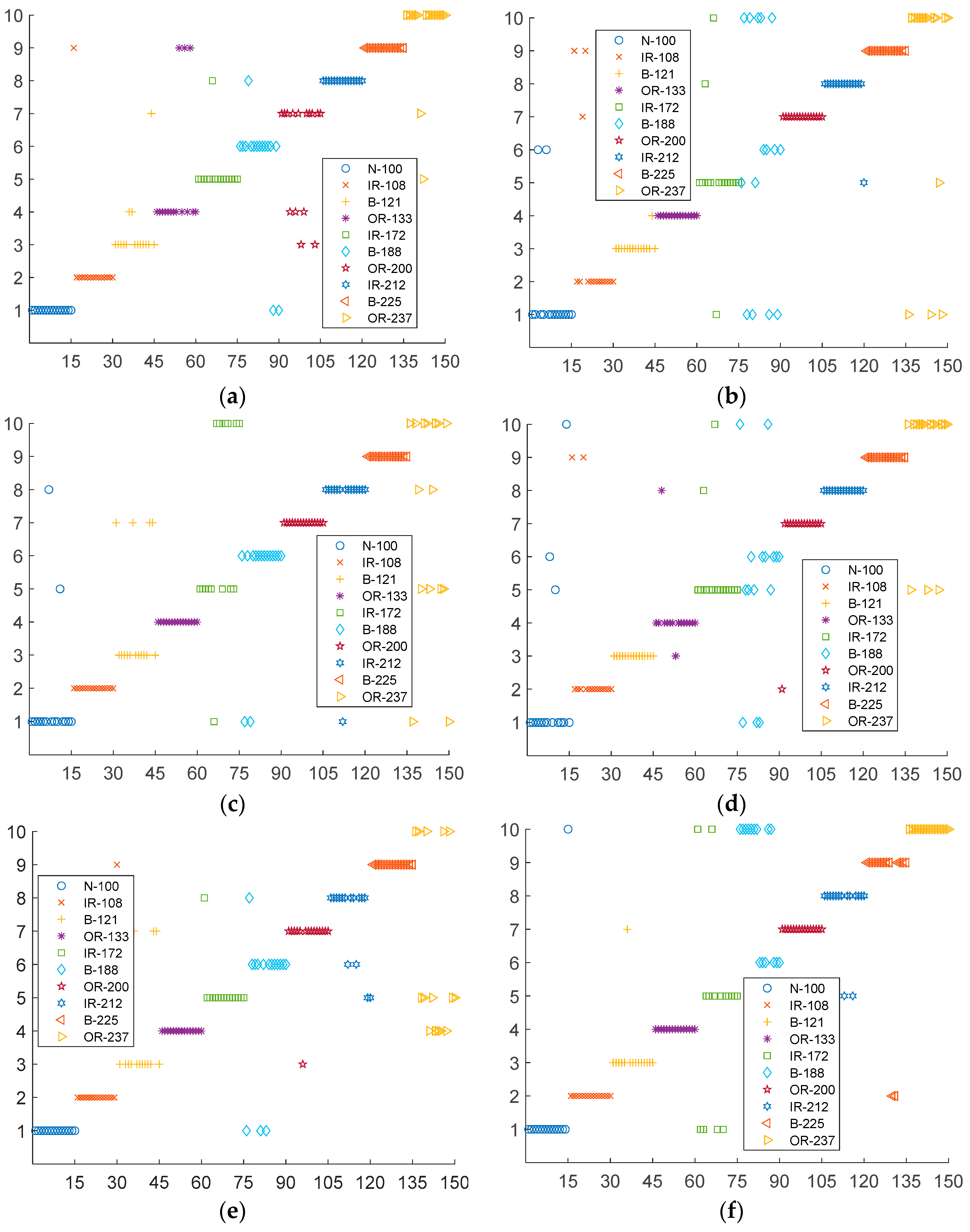
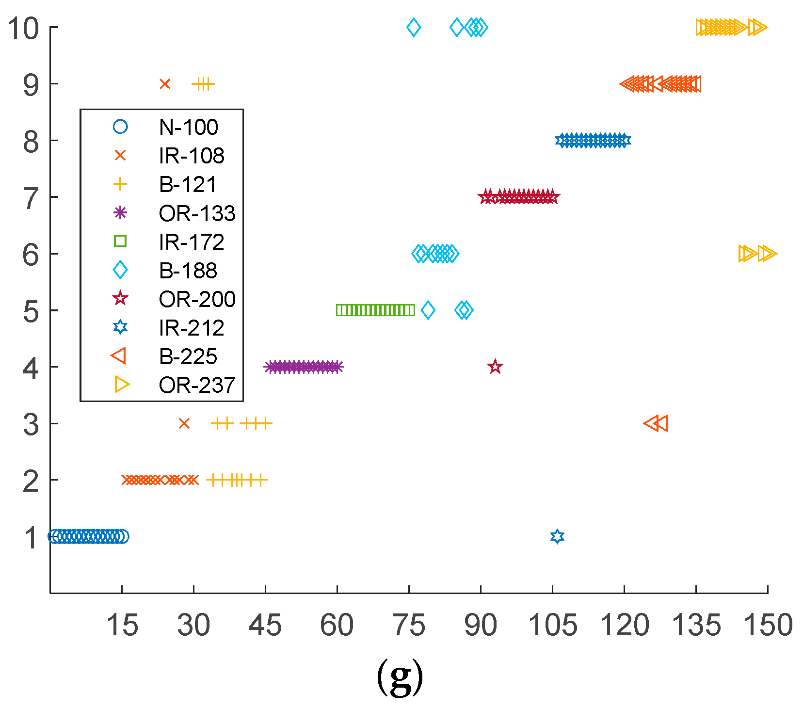
4.2. Feature Distribution
4.3. Classification Effect Verification
5. Double Feature Extraction
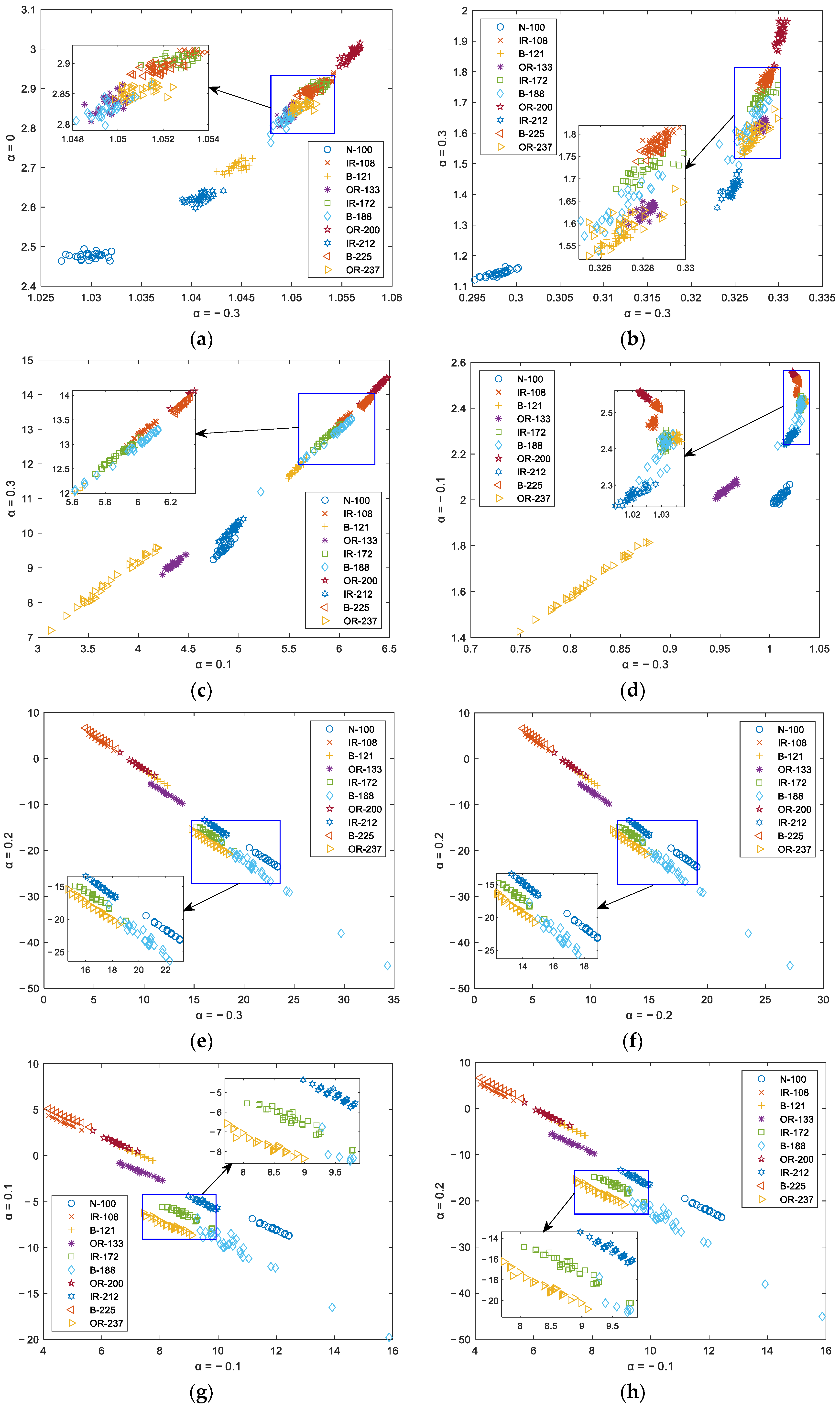
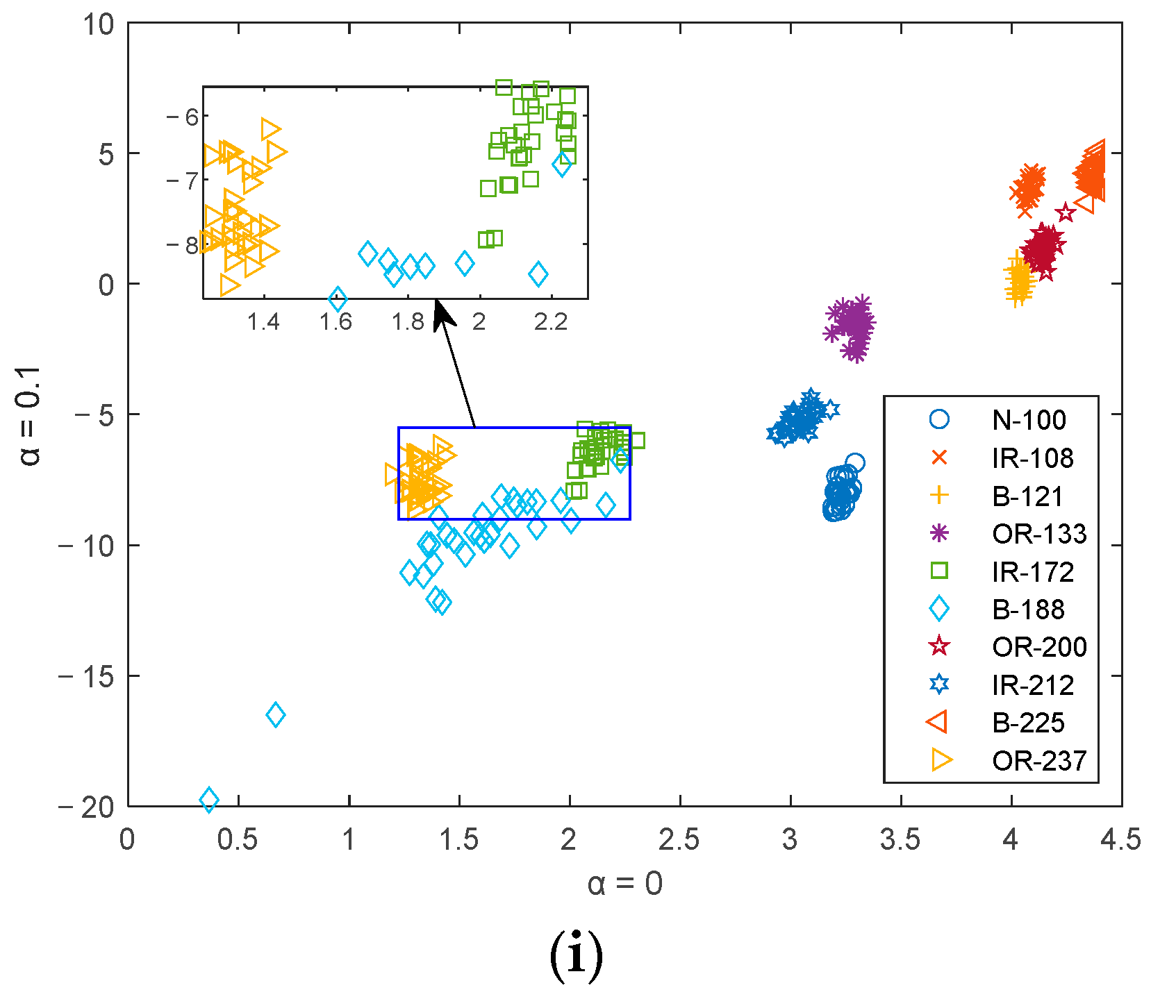
5.1. Feature Distribution
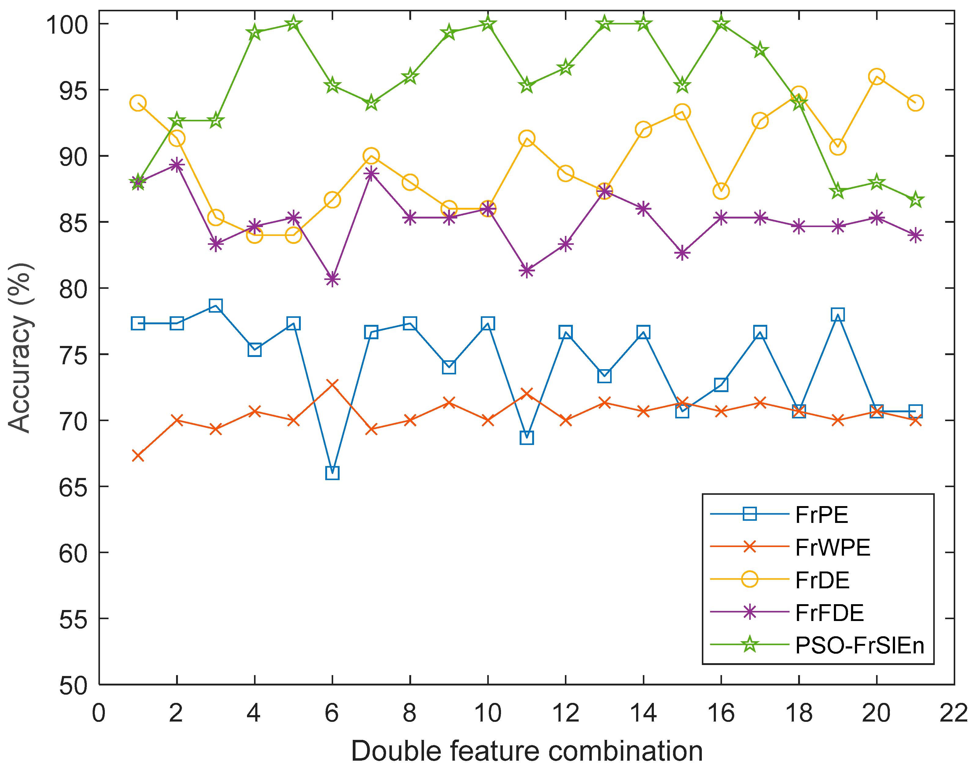
5.2. Classification Effect Verification
6. Conclusions
- (1)
- As an algorithm proposed in 2019, SlEn has not been proposed any improved algorithm. It is proposed for the first time to combine the concept of fractional information with SlEn, and get an improved algorithm of SlEn named FrSlEn.
- (2)
- In order to solve the influence of the two threshold parameters of SlEn on feature significance, PSO is selected to optimize the two threshold parameters, which assists FrSlEn to make the extracted features more significant.
- (3)
- In the experiment of single feature extraction, under any values of α, the classification accuracies of PSO-FrSlEn are the highest. The classification accuracies of PSO-FrSlEn are higher than that of PSO-SlEn, where 88% is the highest classification accuracy of PSO-FrSlEn under α = −0.3. The highest classification accuracy of PSO-FrSlEn is at least 5.33% higher than FrPE, FrWPE, FrDE, and FrFDE.
- (4)
- In the experiment of double feature extraction, the classification accuracies of PSO-FrSlEn under five double feature combinations are 100%. The highest classification accuracies of FrPE, FrWPE, FrDE, and FrFDE are at least 4% less than PSO-FrSlEn, where the highest classification accuracy of FrWPE is 27.33% less than PSO-FrSlEn.
Author Contributions
Funding
Institutional Review Board Statement
Informed Consent Statement
Data Availability Statement
Conflicts of Interest
Nomenclature
| PE | Permutation entropy |
| WPE | Weighted permutation entropy |
| DE | Dispersion entropy |
| FDE | Fluctuation dispersion entropy |
| SlEn | Slope entropy |
| PSO-SlEn | Particle swarm optimization slope entropy |
| FrPE | Fractional permutation entropy |
| FrWPE | Fractional weighted permutation entropy |
| FrDE | Fractional dispersion entropy |
| FrFDE | Fractional fluctuation dispersion entropy |
| FrSlEn | Fractional slope entropy |
| PSO-FrSlEn | Particle swarm optimization fractional slope entropy |
| Fractional order | |
| Embedding dimension | |
| Time lag | |
| Number of classes | |
| NCDF | Normal cumulative distribution function |
| Large threshold | |
| Small threshold | |
| N-100 | Normal signals |
| IR-108 | Inner race fault signals (fault diameter size: 0.007 inch) |
| B-121 | Ball fault signals (fault diameter size: 0.007 inch) |
| OR-133 | Outer race fault signals (fault diameter size: 0.007 inch) |
| IR-172 | Inner race fault signals (fault diameter size: 0.014 inch) |
| B-188 | Ball fault signals (fault diameter size: 0.014 inch) |
| OR-200 | Outer race fault signals (fault diameter size: 0.014 inch) |
| IR-212 | Inner race fault signals (fault diameter size: 0.021 inch) |
| B-225 | Ball fault signals (fault diameter size: 0.021 inch) |
| OR-237 | Outer race fault signals (fault diameter size: 0.021 inch) |
| KNN | K-Nearest Neighbor |
References
- Tsallis, C. Possible generalization of Boltzmann-Gibbs statistics. J. Stat. Phys. 1988, 52, 479–487. [Google Scholar] [CrossRef]
- Rényi, A. On measures of entropy and information. Virology 1985, 142, 158–174. [Google Scholar]
- Yin, Y.; Sun, K.; He, S. Multiscale permutation Rényi entropy and its application for EEG signals. PLoS ONE 2018, 13, 0202558. [Google Scholar] [CrossRef]
- Richman, J.S.; Moorman, J.R. Physiological time-series analysis using approximate entropy and sample entropy. Am. J. Physiol.-Heart Circ. Physiol. 2000, 6, 2039–2049. [Google Scholar] [CrossRef] [Green Version]
- Zair, M.; Rahmoune, C.; Benazzouz, D. Multi-fault diagnosis of rolling bearing using fuzzy entropy of empirical mode decomposition, principal component analysis, and SOM neural network. Proc. Inst. Mech. Eng. Part C 2019, 233, 3317–3328. [Google Scholar] [CrossRef]
- Lin, J.; Lin, J. Divergence measures based on the Shannon entropy. IEEE Trans. Inf. Theory 1991, 37, 145–151. [Google Scholar] [CrossRef] [Green Version]
- Bandt, C.; Pompe, B. Permutation entropy: A natural complexity measure for time series. Phys. Rev. Lett. 2002, 88, 174102. [Google Scholar] [CrossRef]
- Rostaghi, M.; Azami, H. Dispersion Entropy: A Measure for Time Series Analysis. IEEE Signal Process. Lett. 2016, 23, 610–614. [Google Scholar] [CrossRef]
- Tylová, L.; Kukal, J.; Hubata-Vacek, V.; Vyšata, O. Unbiased estimation of permutation entropy in EEG analysis for Alzheimer’s disease classification. Biomed. Signal Process. Control. 2018, 39, 424–430. [Google Scholar] [CrossRef]
- Rostaghi, M.; Ashory, M.R.; Azami, H. Application of dispersion entropy to status characterization of rotary machines. J. Sound Vib. 2019, 438, 291–308. [Google Scholar] [CrossRef]
- Qu, J.; Shi, C.; Ding, F.; Wang, W. A novel aging state recognition method of a viscoelastic sandwich structure based on permutation entropy of dual-tree complex wavelet packet transform and generalized Chebyshev support vector machine. Struct. Health Monit. 2020, 19, 156–172. [Google Scholar] [CrossRef]
- Azami, H.; Escudero, J. Improved multiscale permutation entropy for biomedical signal analysis: Interpretation and application to electroencephalogram recordings. Biomed. Signal Process. Control. 2016, 23, 28–41. [Google Scholar] [CrossRef] [Green Version]
- Zhang, W.; Zhou, J. A Comprehensive Fault Diagnosis Method for Rolling Bearings Based on Refined Composite Multiscale Dispersion Entropy and Fast Ensemble Empirical Mode Decomposition. Entropy 2019, 21, 680. [Google Scholar] [CrossRef] [PubMed] [Green Version]
- Feng, F.; Rao, G.; Jiang, P.; Si, A. Research on early fault diagnosis for rolling bearing based on permutation entropy algorithm. In Proceedings of the IEEE Prognostics and System Health Management Conference, Beijing, China, 23–25 May 2012; Volume 10, pp. 1–5. [Google Scholar]
- Fadlallah, B.; Chen, B.; Keil, A. Weighted-permutation entropy: A complexity measure for time series incorporating amplitude information. Phys. Rev. E 2013, 87, 022911. [Google Scholar] [CrossRef] [PubMed] [Green Version]
- Xie, D.; Hong, S.; Yao, C. Optimized Variational Mode Decomposition and Permutation Entropy with Their Application in Feature Extraction of Ship-Radiated Noise. Entropy 2021, 23, 503. [Google Scholar] [CrossRef]
- Li, D.; Li, X.; Liang, Z.; Voss, L.J.; Sleigh, J.W. Multiscale permutation entropy analysis of EEG recordings during sevoflurane anesthesia. J. Neural Eng. 2010, 7, 046010. [Google Scholar] [CrossRef]
- Deng, B.; Cai, L.; Li, S.; Wang, R.; Yu, H.; Chen, Y. Multivariate multi-scale weighted permutation entropy analysis of EEG complexity for Alzheimer’s disease. Cogn. Neurodyn. 2017, 11, 217–231. [Google Scholar] [CrossRef]
- Zhenya, W.; Ligang, Y.; Gang, C.; Jiaxin, D. Modified multiscale weighted permutation entropy and optimized support vector machine method for rolling bearing fault diagnosis with complex signals. ISA Trans. 2021, 114, 470–480. [Google Scholar]
- Li, R.; Ran, C.; Luo, J.; Feng, S.; Zhang, B. Rolling bearing fault diagnosis method based on dispersion entropy and SVM. In Proceedings of the International Conference on Sensing, Diagnostics, Prognostics, and Control (SDPC), Beijing, China, 15–17 August 2019; Volume 10, pp. 596–600. [Google Scholar]
- Azami, H.; Escudero, J. Amplitude- and Fluctuation-Based Dispersion Entropy. Entropy 2018, 20, 210. [Google Scholar] [CrossRef] [Green Version]
- Zami, H.; Rostaghi, M.; Abásolo, D.; Javier, E. Refined Composite Multiscale Dispersion Entropy and its Application to Biomedical Signals. IEEE Trans. Biomed. Eng. 2017, 64, 2872–2879. [Google Scholar]
- Li, Z.; Li, Y.; Zhang, K. A Feature Extraction Method of Ship-Radiated Noise Based on Fluctuation-Based Dispersion Entropy and Intrinsic Time-Scale Decomposition. Entropy 2019, 21, 693. [Google Scholar] [CrossRef] [PubMed] [Green Version]
- Zheng, J.; Pan, H. Use of generalized refined composite multiscale fractional dispersion entropy to diagnose the faults of rolling bearing. Nonlinear Dyn. 2021, 101, 1417–1440. [Google Scholar] [CrossRef]
- Ali, K. Fractional order entropy: New perspectives. Opt.-Int. J. Light Electron Opt. 2016, 127, 9172–9177. [Google Scholar]
- He, S.; Sun, K. Fractional fuzzy entropy algorithm and the complexity analysis for nonlinear time series. Eur. Phys. J. Spec. Top. 2018, 227, 943–957. [Google Scholar] [CrossRef]
- Cuesta-Frau, D. Slope Entropy: A New Time Series Complexity Estimator Based on Both Symbolic Patterns and Amplitude Information. Entropy 2019, 21, 1167. [Google Scholar] [CrossRef] [Green Version]
- Cuesta-Frau, D.; Dakappa, P.H.; Mahabala, C.; Gupta, A.R. Fever Time Series Analysis Using Slope Entropy. Application to Early Unobtrusive Differential Diagnosis. Entropy 2020, 22, 1034. [Google Scholar] [CrossRef]
- Cuesta-Frau, D.; Schneider, J.; Bakštein, E.; Vostatek, P.; Spaniel, F.; Novák, D. Classification of Actigraphy Records from Bipolar Disorder Patients Using Slope Entropy: A Feasibility Study. Entropy 2020, 22, 1243. [Google Scholar] [CrossRef]
- Li, Y.; Gao, P.; Tang, B. Double Feature Extraction Method of Ship-Radiated Noise Signal Based on Slope Entropy and Permutation Entropy. Entropy 2022, 24, 22. [Google Scholar] [CrossRef]
- Shi, E. Single Feature Extraction Method of Bearing Fault Signals Based on Slope Entropy. Shock. Vib. 2022, 2022, 6808641. [Google Scholar] [CrossRef]
- Case Western Reserve University. Available online: https://engineering.case.edu/bearingdatacenter/pages/welcome-case-western-reserve-university-bearing-data-center-website (accessed on 17 October 2021).


| Figure | FrPE Accuracy (%) | FrWPE Accuracy (%) | FrDE Accuracy (%) | FrFDE Accuracy (%) | PSO-FrSlEn Accuracy (%) |
|---|---|---|---|---|---|
| −0.3 | 64.67 | 46.67 | 82.67 | 77.33 | 88 |
| −0.2 | 78.67 | 60.67 | 81.33 | 73.33 | 84 |
| −0.1 | 76.67 | 66.67 | 80.67 | 79.33 | 83.33 |
| 0 | 76.67 | 69.33 | 69.33 | 79.33 | 81.33 |
| 0.1 | 75.33 | 69.33 | 80 | 79.33 | 86 |
| 0.2 | 75.33 | 69.33 | 82 | 80.67 | 85.33 |
| 0.3 | 66 | 72.76 | 82.67 | 80 | 83.33 |
| Entropy | Fractional Order Combinations | Accuracy (%) |
|---|---|---|
| FrPE | 78.67 | |
| FrWPE | 72.67 | |
| FrDE | 96 | |
| FrFDE | 89.33 | |
| PSO-FrSlEn | 100 | |
| 100 | ||
| 100 | ||
| 100 | ||
| 100 |
Publisher’s Note: MDPI stays neutral with regard to jurisdictional claims in published maps and institutional affiliations. |
© 2022 by the authors. Licensee MDPI, Basel, Switzerland. This article is an open access article distributed under the terms and conditions of the Creative Commons Attribution (CC BY) license (https://creativecommons.org/licenses/by/4.0/).
Share and Cite
Li, Y.; Mu, L.; Gao, P. Particle Swarm Optimization Fractional Slope Entropy: A New Time Series Complexity Indicator for Bearing Fault Diagnosis. Fractal Fract. 2022, 6, 345. https://0-doi-org.brum.beds.ac.uk/10.3390/fractalfract6070345
Li Y, Mu L, Gao P. Particle Swarm Optimization Fractional Slope Entropy: A New Time Series Complexity Indicator for Bearing Fault Diagnosis. Fractal and Fractional. 2022; 6(7):345. https://0-doi-org.brum.beds.ac.uk/10.3390/fractalfract6070345
Chicago/Turabian StyleLi, Yuxing, Lingxia Mu, and Peiyuan Gao. 2022. "Particle Swarm Optimization Fractional Slope Entropy: A New Time Series Complexity Indicator for Bearing Fault Diagnosis" Fractal and Fractional 6, no. 7: 345. https://0-doi-org.brum.beds.ac.uk/10.3390/fractalfract6070345