Salience Bias and Overwork

Abstract

In this study, we enrich a standard principal–agent model with hidden action by introducing salience-biased perception on the agent’s side. The agent’s misguided focus on salient payoffs, which leads the agent’s and the principal’s probability assessments to diverge, has two effects: First, the agent focuses too much on obtaining a bonus, which facilitates incentive provision. Second, the principal may exploit the diverging probability assessments to relax participation. We show that salience bias can reverse the nature of the inefficiency arising from moral hazard; i.e., the principal does not necessarily provide insufficient incentives that result in inefficiently low effort but instead may well provide excessive incentives that result in inefficiently high effort.

1. Introduction

One of the iconic workhorse models of modern contract theory used to analyze incentive provision and work effort is the moral hazard model with hidden action where both the principal and the wealth-constrained agent have linear utility functions for money.1 This model, which dates back to work by Innes [2], Baliga and Sjöström [3], and Pitchford [4], has become increasingly popular and was, despite its simplicity, fruitfully applied to a plethora of topics relevant for economics and management science.2 The key insight of the basic static moral hazard model with hidden action is that the principal provides the agent with inefficiently low incentives, which results in the agent exerting inefficiently low effort, i.e., “underwork” prevails.

The model’s singular focus on the agent’s work effort being too low, however, seems disconcerting given that several studies point to overwork as a very serious problem. For example, conducting telephone interviews with 1003 wage and salaried employees in the U.S. workforce, the representative study by Galinsky et al. [22] finds that 44% of U.S. employees were overworked or felt overwhelmed by how much work they had to do. Furthermore, Galinsky et al. [22] find that a higher degree of being overworked is associated with the experience of higher levels of stress and of a higher number of symptoms of clinical depression, which other studies have associated with non-negligible personal costs for the overworked employee such as health costs or a strain on their family life.3 Notably, the causes for employees being overworked seem primarily rooted in employees exerting effort on non-contractable aspects of their respective employment relationship, such as moving quickly from task to task with little time for recovery between tasks, being permanently accessible by cell phone or email outside normal work hours, or continuing work during their holidays in order to keep up with the demands of their job. In order to devise meaningful measures to prevent (or at least reduce) overwork, it seems worthwhile, if not necessary, to first explore what channels potentially give rise to inefficiently high incentive provision and, as a consequence, inefficiently high effort. In order to address this question, we use the iconic moral hazard model with hidden action, where the principal and a wealth-constrained agent both have linear utility functions for money. This model allows to step away from risk-sharing motives and thus to focus on inefficient effort provision.

To this end, in this paper, we extend the simplest version of said model by allowing the agent’s perception of occurrence probabilities to be blurred by the salience of the associated outcomes. According to salience theory as set out by Bordalo et al. [25], a decision maker’s attention is unknowingly drawn toward (away from) very salient (rather non-salient) outcomes, which leads to the occurrence probabilities of these outcomes being perceived as inflated (deflated). This implies that the agent inflates the probabilities of those states in which his effort choice has an actual impact on his wage. In other words, the agent may focus too much on receiving a high wage (i.e., obtaining a bonus payment) which facilitates incentive provision. Moreover, the agent’s biased probability assessment differs from the objective assessment held by the principal. The principal may exploit these diverging assessments between her and the agent in order to relax the participation constraint. We show that this salience-induced misperception may reverse the nature of the inefficiency compared with the standard model, i.e., that overwork can prevail. Notably, overwork (but not underwork) may occur even in situations where, in the standard model, the first-best effort is always implemented.4

At first glance, it might seem at odds with our model that a salience-biased agent feels overworked, as found in the study by Galinsky et al. [22], as he himself considers accepting the principal’s contract offer and exerting high effort as the optimal course of action at the moment when he makes these decisions. As we will come to understand, however, if the agent exerts a high level of effort under the optimal contract, then either the participation constraint or the incentive compatibility constraint is binding. A reduction in the agent’s salience bias (i.e., a reduction in the agent’s focus on receiving the bonus payment) would then lead to either the agent rejecting the contract in question or the agent exerting low rather than high effort under said contract. Thus, if the salience-induced misdirection of the agent’s attention to certain aspects of a particular decision fades out once the decision has been taken, the agent, in retrospect, may realize that he has overextended himself in the past by exerting more effort than he now deems worthwhile or by agreeing to accept the principal’s contract offer in the first place.

The rest of this paper is structured as follows: After surveying the related literature, we present our model of moral hazard with hidden action and salience-biased perception in Section 2. In Section 3 we analyze the impact of salience bias on incentive provision. We conclude in Section 4. Proofs are deferred to the Appendix A.

Related Literature

Our paper, which incorporates salience theory for choice under risk [25] into an otherwise standard textbook model of static moral hazard with hidden action, adds to two strands of literature. First, our analysis contributes to the vast literature that explores incentive provision in situations with moral hazard. Irrespective of whether the trade-off between efficiency and rent-extraction or the trade-off between incentive provision and risk sharing [28,29] is analyzed, in this literature, underwork is the predominant prediction. In contrast to our paper, the few extant contributions that provide an explanation for overwork rely on a dynamic principal–agent relationship. Analyzing a two-period model, Kräkel and Schöttner [30] find that the agent being replaceable can result in excessive effort (i.e., overwork) in the first period.5 Englmaier et al. [32] find that excessive effort can also occur in a relational contract between a rational principal and a naïve present-biased agent. In that case, if limited liability imposes a binding restriction, the principal may optimally resort to extracting the agent’s rent by inducing the agent to work harder than the efficient effort level (and harder than an agent without a present bias). We complement these contributions by showing that overwork can also prevail in a static one-shot interaction of the principal and the agent.6

Second, our paper adds to the growing literature on applied theoretical models that incorporate salience theory. By now, there is a plethora of contributions that apply salience theory for risk-less consumer choice [34] in models of industrial organization.7 In particular, regarding applications with an incentive-theoretical flavor, Adrian [36] analyzes the screening problem of a monopolist who deals with a salience-biased consumer in an adverse selection environment. Incentive theoretical contributions of salience theory for choice under risk [25], on the other hand, are rather scarce and so far restricted to law-and-economics literature. Specifically, Friehe and Pham [37] analyze the settling behavior of salience-biased defendants, and Mungan [38] explores whether the certainty of a fine or the severity of a fine has a higher deterrent effect on salience-biased offenders. Our paper complements the aforementioned contributions by providing the first analysis of the impact of salience bias on incentive provision and efficiency in a situation with moral hazard, where the agent makes his choice under risk.

Apart from these two strands of literature, conceptually closest to our paper is the analysis in de la Rosa [39], which incorporates an overconfident agent with biased probability assessment into an otherwise standard static moral hazard model. Specifically, the overconfident agent overestimates the marginal contribution of his effort on the probability of success and thus behaves similar to an agent who has a misguided focus on salient payoffs. As a consequence, according to de la Rosa [39], the agent’s overconfidence may help the principal to satisfy incentive compatibility or participation. Importantly, while the diverging probability assessments of the agent and the principal are exogenously given in de la Rosa [39], they are endogenously determined in our setup by the interplay of the agent’s salience-biased perception and the specifics of the contract offered by the principal. Moreover, we abstract from risk-sharing motives and assume that the agent is protected by limited liability, whereas de la Rosa [39] assumes that the agent is risk-averse but with deep pockets. Not surprisingly, de la Rosa [39] therefore focuses on how the agent’s overconfidence affects the trade-off between risk sharing and incentive provision, whereas our analysis explores how a salience-biased probability assessment affects the agent’s limited-liability rent. Finally, and most importantly, de la Rosa [39] defines the first-best outcome as the maximization of the principal’s expected profit plus the agent’s perceived (i.e., biased) expected utility, whereas we consider salience-induced distortions as a bias that should not obtain any normative weight. Due to these diverging definitions of the first-best outcome, de la Rosa [39] cannot answer the question under which circumstances we observe excessive incentives and overwork.

2. Model

2.1. Effort and Production

A principal (P) wants to hire an agent (A) to work on a task on her behalf. The value V generated by A accrues to P and can be either low, $V=V_L$, or high, $V=V_H$, where $0<V_L<V_H$. If A exerts effort $e\in \{0,1\}$, he incurs non-monetary cost $\Psi \left(e\right)=\psi e$, where $\psi >0$.8 As can be seen from

Table 1. Dependence of value V on effort e and state of the world s.

	$\mathit{s}=1$	$\mathit{s}=2$	$\mathit{s}=3$
$e=0$	$V_L$	$V_L$	$V_H$
$e=1$	$V_L$	$V_H$	$V_H$

, the actual realization of the value V depends on A’s effort choice $e\in \{0,1\}$ and which state $s\in \mathcal{S}\equiv \{1,2,3\}$ of three possible, mutually exclusive states is the true state of the world. Specifically, letting the actual realization of the value being denoted by $V(e,s)$, we obtain $V(e,1)=V_L$ and $V(e,3)=V_H$ for all $e\in \{0,1\}$, i.e., the realized value is invariably low in state 1 and invariably high in state 3. In state 2, on the other hand, the realized value is low if A exerted low effort and high if A exerted high effort, i.e., $V(0,2)=V_L$ and $V(1,2)=V_H$. The probability of state $s\in \mathcal{S}$ being the true state of the world is $p_s\in (0,1)$, where ${\sum }_{s\in \mathcal{S}}{p}_s=1$.9

2.2. Information and Contracts

Neither A’s effort choice nor the realization of the state of the world is verifiable. The realization of value V is verifiable. Hence, a contract specifies a transfer t from P to A, which is conditional on the realization of the value V. As the value V is a function of e and s, the transfer t is effectively also a function of e and s. Specifically,

$$\begin{array}{c}\hfill t(e,s)= \left\{\begin{array}{cc}{t}_L\hfill & \mathrm{if}V(e,s)=V_L,\hfill \\ t_H\hfill & \mathrm{if}V(e,s)=V_H.\hfill \end{array}\right.\end{array}$$

(1)

The agent is protected by limited liability such that $t_L$ and $t_H$ must not be below $\overline{t}\in \mathbb{R}$. In order to ensure that a contract is offered in equilibrium, we assume that $\overline{t}\le V_L$.

2.3. Sequence of Events

First, P makes a take-it-or-leave-it contract offer to A, which A decides to accept or reject. Second, if A accepts the offer, he decides which effort $e\in \{0,1\}$ to exert. Thereafter, the state of the world $s\in \mathcal{S}$ and, thus, the value $V(e,s)$ is realized, and the transfer $t(e,s)$ is paid. If A rejects the offer, each party obtains her/his outside option that yields a reservation utility equal to zero.

2.4. Preferences and Salience Bias

Both P and A have a linear utility function for monetary outcomes. The principal perceives the occurrence probabilities of the three states correctly, and her expected value from signing a contract that stipulates transfers $t_L$ and $t_H$ and under which A exerts effort $e\in \{0,1\}$ is given by

$$\begin{array}{c}\hfill U_P(t_L,t_H,e)=\sum _{s\in \mathcal{S}}{p}_s\left[V(e,s)-t(e,s)\right].\end{array}$$

(2)

The agent’s perception of the occurrence probabilities of the three states is blurred by the salience of the respective outcome combinations in the spirit of salience theory [25]. Specifically, A’s expected value from signing a contract that stipulates $t_L$ and $t_H$ and under which he exerts $e\in \{0,1\}$ is given by

$$\begin{array}{c}\hfill U_A(t_L,t_H,e)=\sum _{s\in \mathcal{S}}{\pi }_s\left[t(e,s)-\Psi \left(e\right)\right],\end{array}$$

(3)

where

$$\begin{array}{c}\hfill {\pi }_s=\frac{{\delta }^{k_s}}{{\sum }_{s^{\prime }\in \mathcal{S}}{\delta }^{k_{s^{\prime }}}{p}_{s^{\prime }}}·p_s\mathrm{with}\delta \in (0,1).\end{array}$$

(4)

Here, ${\pi }_s\in (0,1)$ with ${\sum }_{s\in \mathcal{S}}{\pi }_s=1$ is the decision weight that A attaches to state $s\in \mathcal{S}$, $\delta \in (0,1)$ denotes the (inverse) degree of salience bias, and $k_s\in {\mathbb{N}}_{>0}$ denotes the salience rank of state $s\in \mathcal{S}$. The salience ranking starts at 1, has no jumps, and a lower salience rank denotes higher salience. Hence, above-average (below-average) salience translates into the respective state’s objective occurrence probability being perceived as inflated (deflated). Notably, the standard model with A being a risk-neutral expected utility maximizer is captured by $\delta =1$, in which case A perceives the occurrence probabilities correctly. 10

We assume that a state’s salience is fully determined by the contractually specified transfers that A might receive in that state.11 Formally, letting $\sigma (·,·)$ denote the salience function, we obtain $k_s⋚k_{s^{\prime }}$ if and only if $\sigma (t(0,s),t(1,s))⋛\sigma (t(0,s^{\prime }),t(1,s^{\prime }))$ for all $s,s^{\prime }\in \mathcal{S}$. The function $\sigma (·,·)$ is symmetric (i.e., $\sigma (t,t^{\prime })=\sigma (t^{\prime },t)$ for all $t,t^{\prime }\in \mathbb{R}$), assigns identical values to states in which the transfers for both effort levels coincide (i.e., $\sigma (t,t)=\sigma (t^{\prime },t^{\prime })$ for all $t,t^{\prime }\in \mathbb{R}$), and satisfies the following “ordering” property, which captures psychological contrast effects:12

(O)

For all $t,t^{\prime },t^{″},t^{‴}\in \mathbb{R}$, if $[min\{t,t^{\prime }\},max\{t,t^{\prime }\}]⊊[min\{t^{″},t^{‴}\},max\{t^{″},t^{‴}\}]$, then $\sigma (t,t^{\prime })<\sigma (t^{″},t^{‴})$.

Hence, $k_1=k_3\ge k_2$ with the inequality being strict in the case of performance-dependent pay (i.e., for $t_L\ne t_H$). In other words, for performance-independent pay ($t_L=t_H$), A perceives the probabilities correctly, i.e., ${\pi }_s=p_s$ for $s=1,2,3$. For performance-dependent pay ($t_L\ne t_H$), A focuses too much on (over-weighs) state $s=2$, where payments are different, and puts too little attention on (under-weighs) states $s=1$ and $s=3$, where payments are identical. Formally,

$$\begin{array}{c}\hfill {\pi }_2=\frac{1}{p_2+\delta (p_1+p_3)}{p}_2>p_2\mathrm{and}{\pi }_i=\frac{\delta }{p_2+\delta (p_1+p_3)}{p}_i<p_i\mathrm{for}i=1,3.\end{array}$$

(5)

2.5. Benchmark 1: First-Best Effort

Similar to overconfidence, salience bias represents an unknowing mistake in the assessment of the decision environment. Therefore, in the spirit of the literature that studies transactions in the presence of overconfidence [47,48,49], our welfare criterion is the unweighted sum of unbiased (expected) utilities, which corresponds to the expected material gains from trade:

$$G\left(e\right)=\sum _{s\in \mathcal{S}}{p}_s\left[V(e,s)-\Psi \left(e\right)\right].$$

Observation 1.

The first-best effort level $e^{FB}=arg{max}_{e\in \{0,1\}}G\left(e\right)$ is given by

$$e^{FB}= \left\{\begin{array}{cc}1\hfill & \mathrm{if}{\Delta }^{FB}\le V_H-V_L,\hfill \\ 0\hfill & \mathrm{if}{V}_H-V_L\le {\Delta }^{FB},\hfill \end{array}\right.\mathrm{where}{\Delta }^{FB}:=\frac{\psi }{p_2}.$$

Proof. 

See Laffont and Martimort [41]. □

Intuitively, high effort rather than low effort should be exerted if the associated increase in the expected “extra value”, $p_2(V_H-V_L)$, weakly exceeds the associated increase in effort cost, $\psi$.

3. Analysis

When making her contract offer, P must decide which effort level, $e\in \{0,1\}$, she wants to induce and what transfers, $t_L$ and $t_H$, she wants to contractually specify in order to maximize her expected profit. Formally, she solves the following optimization program:

$$\begin{array}{cc}\hfill \underset{e,t_L,t_H}{max}& U_P(t_L,t_H,e)\hfill \end{array}$$

subject to

$$\begin{array}{c}{U}_A(t_L,t_H,e)\ge U_A(t_L,t_H,e^{\prime })\mathrm{for}{e}^{\prime }\in \{0,1\},e\ne e^{\prime }\hfill \end{array}$$

(IC_e) 

$$\begin{array}{cc}\hfill & U_A(t_L,t_H,e)\ge 0\hfill \end{array}$$

(P_e) 

$$\begin{array}{cc}\hfill & t_L\ge \overline{t},t_H\ge \overline{t}.\hfill \end{array}$$

(LL)

The incentive compatibility constraint (IC${}_e$), the participation constraint (P${}_e$), and the limited liability constraint (LL) bear the usual interpretation.

In order to explore the implications of salience bias for effort provision, we will follow the approach pioneered by Grossman and Hart [29] and decompose P’s optimization program into two steps. First, for each effort level, we identify the “cost-minimizing” transfer payments; i.e., those transfer payments that implement the respective effort level at the lowest possible expected transfer payment. Thereafter, in order to determine the overall optimal contract, we compare P’s expected utility across effort levels, given that each effort level is implemented with the respective cost-minimizing transfers. Before launching into this analysis, however, as a second benchmark, we briefly review the outcome of the principal–agent relationship in the absence of salience bias.

3.1. Benchmark 2: No Salience Bias

Without salience bias (i.e., for $\delta =1$), A perceives the probabilities correctly and thus is risk neutral. Letting $\tilde{e}$ denote the effort level that P optimally implements in the absence of salience bias, the outcome of the interaction between P and A takes the following form:

Observation 2.

The principal implements high effort ($\tilde{e}=1$) if and only if $\tilde{\Delta }\le V_H-V_L$, where

$$\begin{array}{c}\hfill \tilde{\Delta }:= \left\{\begin{array}{cc}\frac{p_2+p_3}{p_2}{\Delta }^{FB}\hfill & \mathrm{if}-\frac{p_3}{p_2}\psi <\overline{t},\hfill \\ {\Delta }^{FB}\hfill & \mathrm{if}\overline{t}\le -\frac{p_3}{p_2}\psi .\hfill \end{array}\right.\end{array}$$

(6)

Proof. 

See Laffont and Martimort [41]. □

Intuitively, if $\overline{t}$ is sufficiently low (i.e., if $\overline{t}\le -\frac{p_3}{p_2}\psi$), then limited liability does not impose a binding restriction, and, irrespective of which effort level P implements, A’s expected utility will equal his reservation utility. In this case, P’s problem boils down to maximizing the expected material gains from trade $G(·)$, and, thus, she induces A to exert the materially efficient effort level, i.e., $\tilde{e}=e^{FB}$. Formally, this follows from $\tilde{\Delta }$ being equal to ${\Delta }^{FB}$.

If, on the other hand, $\overline{t}$ is sufficiently high (i.e., if $\overline{t}>-\frac{p_3}{p_2}\psi$), then limited liability imposes a binding restriction. As a consequence, in case high effort is implemented, the agent does not only receive the minimum wage, $\overline{t}$, or is compensated for his outside option, but he obtains an information rent, which is rooted in the necessity to induce high effort by specifying a sufficiently high bonus payment for good performance ($t_H=\frac{\psi }{p_2}+\overline{t}>\overline{t}=t_L$). Thus, P now trades off maximizing the expected gains from trade and cutting back on A’s information rent, which leads to P implementing high effort “less often” than is materially efficient. This well-known result of underwork formally follows from $\tilde{\Delta }$ being strictly smaller than ${\Delta }^{FB}$. Here, if ${\Delta }^{FB}\le V_H-V_L<\tilde{\Delta }$, then $\tilde{e}<e^{FB}$. In summary, in the standard model without salience bias, it is impossible for overwork to prevail.

3.2. Cost-Minimizing Transfers with Salience Bias

The cost-minimization problem for a given effort $e\in \{0,1\}$ is as follows:

$$\begin{array}{c}\hfill \underset{(t_L,t_H)\in {\mathbb{R}}^2}{min}{p}_1{t}_L+p_2[(1-e)t_L+e{t}_H]+p_3{t}_H\mathrm{subject}\mathrm{to}(\mathrm{IC}{}_e),(\mathrm{P}{}_e),\left(\mathrm{LL}\right).\end{array}$$

(7)

In the main section of this paper, we are going to provide an intuitive derivation of the cost-minimizing transfer combination based on a graphical analysis. To this end, consider the isocost curve associated with the expected transfer payment T, given effort level e, i.e., the geometric location in $(t_L,t_H)$—space of all transfer combinations $(t_L,t_H)$ that results in the same expected transfer payment T given A exerts effort e. Formally, this isocost curve is described by

$$\begin{array}{c}\hfill \Gamma \left(t_L\right|e,T)=\frac{T}{e{p}_2+p_3}-\frac{p_1+(1-e)p_2}{e{p}_2+p_3}{t}_L.\end{array}$$

(8)

From (8), it follows that the family of isocost curves comprises parallel, negatively sloped straight lines. Importantly, an isocost curve with a smaller vertical intercept is associated with a strictly lower expected transfer payment than an isocost curve with a greater vertical intercept. As a consequence, the solution to the above cost-minimization problem is a transfer combination $(t_L^e,t_H^e)$ that satisfies (IC${}_e$), (P${}_e$), and (LL) such that there is no other transfer combination $({\widehat{t}}_L,{\widehat{t}}_H)$ that satisfies (IC${}_e$), (P${}_e$), and (LL) and lies on a lower isocost curve than $(t_L^e,t_H^e)$.

3.2.1. Implementation of High Effort ($e=1$)

If P induces $e=1$, then (IC${}_1$) and (P${}_1$) take the following form:

$$t_H\ge {\displaystyle \frac{\psi }{{\pi }_2}}+t_L=:{\Phi }_1^{IC}\left(t_L\right)$$

(IC₁) 

$$t_H\ge {\displaystyle \frac{\psi }{{\pi }_2+{\pi }_3}}-{\displaystyle \frac{{\pi }_1}{{\pi }_2+{\pi }_3}}{t}_L=:{\Phi }_1^P\left(t_L\right).$$

(P₁) 

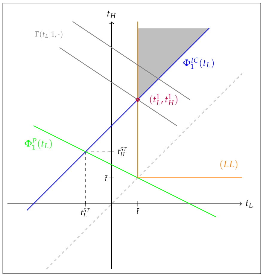
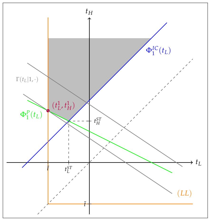
As becomes apparent from (IC${}_1$), for a contract to be incentive compatible, the transfer $t_H$ must be sufficiently higher than the transfer $t_L$. Figure 1 and Figure 2 depict the functions ${\Phi }_1^{IC}\left(t_L\right)$ and ${\Phi }_1^P\left(t_L\right)$ in $(t_L,t_H)$-space together with the (LL) constraint. The (LL) constraint requires $(t_L,t_H)$ to be located to the north-east of the orange L-shaped curve, the kink of which lies on the 45 degree line. Notably, $d\Gamma \left(t_L\right|1,·)/d{t}_L<d{\Phi }_1^P\left(t_L\right)/d{t}_L$. The gray-shaded areas in Figure 1 and Figure 2 represent the set of transfer combinations that jointly satisfy (IC${}_1$), (P${}_1$), and (LL) for $\overline{t}\ge t_L^{ST}$ and $\overline{t}<t_L^{ST}$, respectively, where

$$\begin{array}{c}\hfill t_L^{ST}:=-\frac{{\pi }_3}{{\pi }_2}\psi .\end{array}$$

(9)

Here, $t_L^{ST}$ corresponds to the unique value of transfer $t_L$, for which ${\Phi }_1^{IC}(·)$ and ${\Phi }_1^P(·)$ intersect, i.e., denoting the corresponding value of transfer $t_H$ with $t_H^{ST}$. We can obtain ${\Phi }_1^{IC}\left(t_L^{ST}\right)={\Phi }_1^P\left(t_L^{ST}\right)=:t_H^{ST}$. Thus, the transfer combination $(t_L,t_H)=(t_L^{ST},t_H^{ST})$ is the only transfer combination for which both the participation constraint and the incentive compatibility constraint are satisfied with equality.

In fact, the transfer combination $(t_L,t_H)=(t_L^{ST},t_H^{ST})$ will be our staring point to intuitively understand the structure of the cost-minimizing contract in order to implement high effort.

Proposition 1.

The cost-minimizing transfers $t_L^1$ and $t_H^1$ to implement $e=1$ satisfy

$$\begin{array}{c}\hfill t_L^1=\overline{t}\mathrm{and}{t}_H^1= \left\{\begin{array}{cc}\overline{t}+\frac{\psi }{{\pi }_2}\hfill & \mathrm{if}\overline{t}\ge t_L^{ST},\hfill \\ -\frac{{\pi }_1}{{\pi }_2+{\pi }_3}\overline{t}+\frac{\psi }{{\pi }_2+{\pi }_3}\hfill & \mathrm{if}\overline{t}<t_L^{ST}.\hfill \end{array}\right.\end{array}$$

(10)

What is the intuition behind Proposition 1? As usual, the structure of the cost-minimizing contract is shaped by those of the constraints which impose a binding restriction on P’s choice of transfers and which constraints do not. So, we consider the transfer combination $(t_L,t_H)=(t_L^{ST},t_H^{ST})$ for which both the participation constraint and the incentive compatibility constraint are satisfied with equality. If $\overline{t}>t_L^{ST}$, as depicted in Figure 1, this transfer combination violates the limited liability constraint as $t_L=t_L^{ST}<\overline{t}$. Thus, in order to satisfy the limited liability constraint, $t_L$ must be increased. For incentive compatibility to be maintained, however, this requires $t_H$ to be also increased appropriately, and the “cheapest” way to do so is to move to the north-east along the ${\Phi }_1^{IC}(·)$-curve. Notably, with both transfers increasing compared to the transfer combination that we started out from, the participation constraint is slack under this contractual adjustment. As becomes apparent from Figure 1, the cost-minimizing contract is obtained once the transfer $t_L$ just satisfies the requirement imposed by the limited liability constraint (i.e., $t_L^1=\overline{t}$), and the transfer $t_H$ is specified such that the incentive compatibility constraint holds with equality (i.e., $t_H^1={\Phi }_1^{IC}\left(\overline{t}\right)$). Thus, under the cost-minimizing contract it is the limited liability constraint (with regard to transfer $t_L$) and the incentive compatibility constraint that bind, just as would be the case for an unbiased agent if the minimum transfer $\overline{t}$ were sufficiently high. There is, however, one important difference. Since incentive compatibility requires $t_H>t_L$, a salience-biased agent perceives the occurrence probability of state 2 (i.e., where he receives the “bonus payment” $t_H-t_L$ if and only if he exerted high effort) as inflated (i.e., ${\pi }_2>p_2$). On the other hand, the occurrence probabilities of states 1 and 3, where the transfer does not depend on A’s effort choice, are perceived as deflated (i.e., ${\pi }_i<p_i$ for $i=1,3$). As a consequence, the minimum bonus payment necessary to induce high effort is lower for an agent whose perception is blurred by salience bias than for an unbiased agent.

Next, suppose that $\overline{t}<t_L^{ST}$, as depicted in Figure 2. Under the transfer combination $(t_L,t_H)=(t_L^{ST},t_H^{ST})$, for which both the participation constraint and the incentive compatibility constraint are satisfied with equality, the limited liability constraint is slack with regard to both transfers as $\overline{t}<t_L<t_H$. In this case, P can exploit that her own probability assessment and A’s probability assessment diverge by decreasing $t_L$ and increasing $t_H$ in a way such that the participation constraint is still satisfied with equality, i.e., by moving to the north-west along the ${\Phi }_1^P(·)$-curve.13 Compared with the transfer combination that we started out from, with the bonus payment $t_H-t_L$ being increased by this contractual adjustment, the incentive compatibility constraint becomes slack, and A strictly prefers to exert high effort. Nevertheless, P’s expected cost for implementing high effort is strictly reduced. The reason for this is that A, given that he exerts high effort, puts too much weight on the states where he receives the high transfer $t_H$ (i.e., ${\pi }_2+{\pi }_3>p_2+p_3$) and too little weight on the state where he receives the low transfer $t_L$ (i.e., ${\pi }_1<p_1$). As a consequence, the contractual adjustment strictly decreases the actual, objectively expected transfer payment while, at the same time, leaving the expected transfer payment as perceived by A unchanged. Graphically, this is reflected by the fact that the slopes of the isocost curves are steeper than the slope of the ${\Phi }_1^P(·)$ curve. As becomes apparent from Figure 2, the cost-minimizing contract is obtained once the transfer $t_L$ just satisfies the requirement imposed by the limited liability constraint (i.e., $t_L^1=\overline{t}$) and the transfer $t_H$ is specified such that the participation constraint holds with equality (i.e., $t_H^1={\Phi }_1^P\left(\overline{t}\right)$). The exact size of the high transfer $t_H$ depends on A’s degree of salience bias. In particular, the more biased A’s perception is, the lower the cost-minimizing specification of transfer $t_H$.14

The principal’s expected utility under the cost-minimizing contract to implement $e=1$ is

$$\begin{array}{c}{U}_P(t_L^1,t_H^1,1)=p_1{V}_L+(p_2+p_3)V_H\hfill \\ \hfill \hspace{1em}\hspace{1em}\hspace{1em}\hspace{1em}\hspace{1em}\hspace{1em}\hspace{1em}\hspace{1em}\hspace{1em}-\left\{\begin{array}{cc}\left[p_1\overline{t}+(p_2+p_3)\left(\overline{t}+\frac{\psi }{{\pi }_2}\right)\right]\hfill & \mathrm{if}\overline{t}\ge t_L^{ST},\hfill \\ \left[p_1\overline{t}+(p_2+p_3)\left(-\frac{{\pi }_1}{{\pi }_2+{\pi }_3}\overline{t}+\frac{\psi }{{\pi }_2+{\pi }_3}\right)\right]\hfill & \mathrm{if}\overline{t}<t_L^{ST}.\hfill \end{array}\right.\end{array}$$

(11)

An interesting question, which is answered in the following corollary, is whether P can benefit from A’s salience bias.

Corollary 1.

If the degree of salience bias marginally increases (i.e., if δ decreases), then $U_P(t_L^1,t_H^1,1)$ strictly increases.

This comparative static result is quite plausible. An increase in salience bias leads to A attaching even more weight to the state where his effort makes an actual difference to his remuneration (i.e., $\frac{d{\pi }_2}{d\delta }<0$). In the case where the incentive compatibility constraint imposes a binding restriction (high $\overline{t}$), this allows P to decrease the bonus payment for good performance and, thus, to reduce her expected cost. If the incentive compatibility constraint is slack but the participation constraint is binding (low $\overline{t}$), an increase in salience bias allows P to exploit the divergence in prior beliefs even more to her own advantage. The reason for this is that A then attaches even higher value to an increase of $t_H$ and cares even less about a decrease of $t_L$ (i.e., $\frac{d({\pi }_2+{\pi }_3)}{d\delta }<0$).

3.2.2. Implementation of Low Effort ($e=0$)

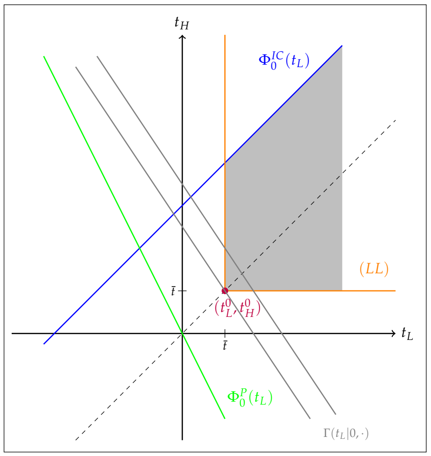
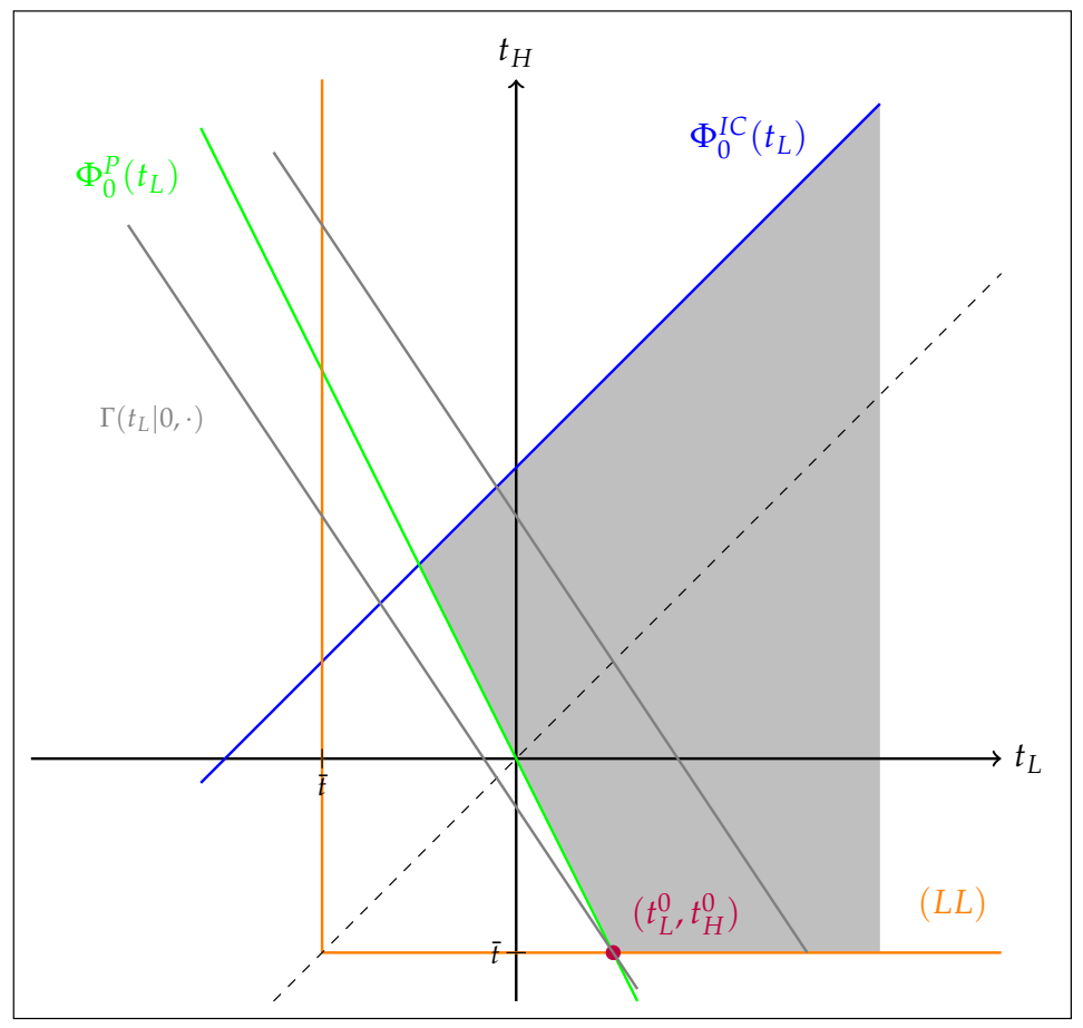
If P induces $e=0$, (IC${}_0$) and (P${}_0$) take the following form:

$$t_H\le {\displaystyle \frac{\psi }{{\pi }_2}}+t_L=:{\Phi }_0^{IC}\left(t_L\right)$$

(IC₀) 

$$t_H\ge -{\displaystyle \frac{{\pi }_1+{\pi }_2}{{\pi }_3}}{t}_L=:{\Phi }_0^P\left(t_L\right).$$

(P₀) 

As depicted in Figure 3 and Figure 4, which are drawn in analogy to Figure 1 and Figure 2, we now have $d{\Phi }_0^P\left(t_L\right)/d{t}_L<d\Gamma \left(t_L\right|0,·)/d{t}_L$.

Proposition 2.

The cost-minimizing transfers $t_L^0$ and $t_H^0$ to implement $e=0$ satisfy

$$\begin{array}{c}\hfill t_L^0= \left\{\begin{array}{cc}\overline{t}\hfill & \mathrm{if}\overline{t}\ge 0,\hfill \\ -\frac{{\pi }_3}{{\pi }_1+{\pi }_2}\overline{t}\hfill & \mathrm{if}\overline{t}<0,\hfill \end{array}\right.and{t}_H^0=\overline{t}.\end{array}$$

(12)

In order to implement low effort, there is no need for P to reward good performance with a bonus payment. Thus, the natural candidates for an optimal contract are transfer payments $t_L$ and $t_H$ that just satisfy the limited liability requirement, i.e., $t_L=t_H=\overline{t}$. If the transfer combination $(t_L,t_H)=(\overline{t},\overline{t})$ satisfies the participation constraint, which is the case if the minimum transfer is sufficiently high (i.e., if $\overline{t}\ge 0$), then it is the optimal contract.

If, on the other hand, the minimum transfer is too low (i.e., if $\overline{t}<0$), then the transfer combination $(t_L,t_H)=(\overline{t},\overline{t})$ does not satisfy the participation constraint. In this case, the participation constraint imposes a binding restriction, and P can exploit the divergence between her own and A’s probability assessments. Specifically, given that A exerts low effort, for $t_L\ne t_H$, he inflates the probability of receiving $t_L$ (i.e., ${\pi }_1+{\pi }_2>p_1+p_2$) and deflates the probability of receiving $t_H$ (i.e., ${\pi }_3<p_3$). As a consequence, an increase in $t_L$ that is accompanied by a decrease in $t_H$ such that the expected transfer payment as perceived by A is left unchanged strictly reduces the actual objectively expected transfer payment. Therefore, as becomes apparent from Figure 4, the cost-minimizing contract is obtained once the transfer $t_H$ just satisfies the requirement imposed by the limited liability constraint (i.e., $t_H^0=\overline{t}$), and the transfer $t_L$ is specified such that the participation constraint holds with equality (i.e., ${\Phi }_0^P\left(t_L^0\right)=\overline{t}$).

The principal’s expected utility under the cost-minimizing contract to implement $e=0$ is

$$U_P(t_L^0,t_H^0,0)=(p_1+p_2)V_L+p_3{V}_H- \left\{\begin{array}{cc}\overline{t}\hfill & \mathrm{if}\overline{t}\ge 0,\hfill \\ \left[(p_1+p_2)\left(-\frac{{\pi }_3}{{\pi }_1+{\pi }_2}\overline{t}\right)+p_3\overline{t}\right]\hfill & \mathrm{if}\overline{t}<0,\hfill \end{array}\right.$$

(13)

and once again, an increase in the degree of A’s salience bias makes P (weakly) better off.

Corollary 2.

If the degree of the agent’s salience bias marginally increases (i.e., if δ decreases), $U_P(t_L^0,t_H^0,0)$ remains unchanged if $\overline{t}\ge 0$ and strictly increases if $\overline{t}<0$.

Clearly, if $\overline{t}\ge 0$, the cost-minimizing transfers are determined by the limited liability constraint (LL) alone, i.e., $t_L^0=t_H^0=\overline{t}$. As a consequence, as the liability threshold $\overline{t}$ remains unchanged, a change in the degree of the agent’s salience bias leaves the cost-minimizing transfers and, thus, the principal’s expected utility unaffected. If $\overline{t}<0$, on the other hand, an increase in the degree of the agent’s salience bias strictly increases the principal’s maximum utility from implementing low effort. In this case the participation constraint is binding, and the contract offered by the principal is a gamble that exploits the diverging probability assessments. An increase in the degree of the agent’s salience bias increases the divergence in prior beliefs and thus allows the principal to exploit this divergence more effectively.

3.3. Second-Best Effort with Salience Bias

Having analyzed the second-best optimal contracts for given effort levels, we can now investigate which effort level is optimally induced by the principal. Let $e^{\ast }=arg{max}_{e\in \{0,1\}}{U}_P(t_L^e,t_H^e,e)$ denote this second-best effort level. As a tie-breaking rule, we assume that P induces high effort when being indifferent, i.e., $e^{\ast }=1$ if and only if $U_P(t_L^1,t_H^1,1)\ge U_P(t_L^0,t_H^0,0)$. Intuitively, P will induce high effort rather than low effort if and only if the associated increase in value is sufficiently high.

Proposition 3.

The principal implements high effort, i.e., $e^{\ast }=1$, if and only if $\Delta \left(\overline{t}\right)\le V_H-V_L$, where

$$\begin{array}{c}\hfill \Delta \left(\overline{t}\right):= \left\{\begin{array}{cc}\frac{p_2+p_3}{{\pi }_2}{\Delta }^{FB}\hfill & \mathrm{if}0\le \overline{t},\hfill \\ \frac{p_2+p_3}{{\pi }_2}{\Delta }^{FB}+\frac{p_1+p_2}{p_2({\pi }_1+{\pi }_2)}\overline{t}\hfill & \mathrm{if}{t}_L^{ST}\le \overline{t}<0,\hfill \\ \frac{p_2+p_3}{{\pi }_2+{\pi }_3}{\Delta }^{FB}-\frac{\overline{t}}{p_2}\left(\frac{1-p_1}{1-{\pi }_1}-\frac{1-p_3}{1-{\pi }_3}\right)\hfill & \mathrm{if}\overline{t}<t_L^{ST}.\hfill \end{array}\right.\end{array}$$

(14)

We are interested in the distortion that arises under the second-best optimal contract, and whether this is caused by the (degree of) salience bias. According to Proposition 3, how $\Delta \left(\overline{t}\right)$ relates to ${\Delta }^{FB}$ depends on the liability threshold ($\overline{t}$), the objective occurrence probabilities ($p_1$, $p_2$, and $p_3$), and the degree of salience bias ($\delta$), which enters into the decision weights (${\pi }_1$, ${\pi }_2$, and ${\pi }_3$).

Recall that, for $\overline{t}\ge 0$, the second-best optimal contract that implements $e=0$ is independent of the salience bias. On the other hand, implementing $e=1$ becomes cheaper, the stronger the salience bias, and thus the excess weight on receiving the bonus payment, is. Not surprisingly, if the agent’s probability assessment is distorted, high effort is implemented “more often” compared to the standard case without salience bias ($\delta =1$). Interestingly, the salience bias can make the implementation of high effort so cheap, that P induces high effort even in cases where low effort maximizes the undistorted gains from trade. To see this formally, note that for $\overline{t}\ge 0$, $\Delta \left(\overline{t}\right)⋚{\Delta }^{FB}$ if and only if $\frac{p_2+p_3}{{\pi }_2}⋚1$, which is equivalent to

$$\delta ⋚\frac{p_1{p}_2}{(1-p_1)(1-p_2)}\in (0,1).$$

(15)

This observation already shows how salience bias can fundamentally alter the outcome of the principal–agent relationship in comparison with the standard model without salience bias. In the standard model with an unbiased agent (i.e., $\delta =1$), we have $\Delta \left(\overline{t}\right)=\tilde{\Delta }=(1+\frac{p_3}{p_2}){\Delta }^{FB}>{\Delta }^{FB}$, such that any distortion in effort must take the form of underwork (i.e., $\tilde{e}<e^{FB}$). In contrast, if A’s perception is sufficiently blurred by salience, then P induces high effort even though the gains from trade are maximized by low effort; i.e., if $\delta <\frac{p_1{p}_2}{(1-p_1)(1-p_2)}$ and $\Delta \left(\overline{t}\right)\le V_H-V_L<{\Delta }^{FB}$, then the distortion in effort takes the form of overwork (i.e., $e^{\ast }>e^{FB}$).

For $\overline{t}<0$, P benefits from A’s distorted probability assessments irrespective of whether she induces high or low effort. This makes the comparison of $\Delta \left(\overline{t}\right)$ and ${\Delta }^{FB}$ more complicated and significantly less tractable. To retain tractability and to streamline the exposition, we impose the following simplifying assumption:

Assumption 1.

$p_2=p\in (0,1)$ and $p_1=p_3=\frac{1-p}{2}$.

According to Assumption 1, states 1 and 3, where the agent’s effort choice has no impact on the value that is generated for the principal, are equiprobable. If Assumption 1 holds, how $\Delta \left(\overline{t}\right)$ compares to ${\Delta }^{FB}$ can be related to the degree of salience bias as follows:

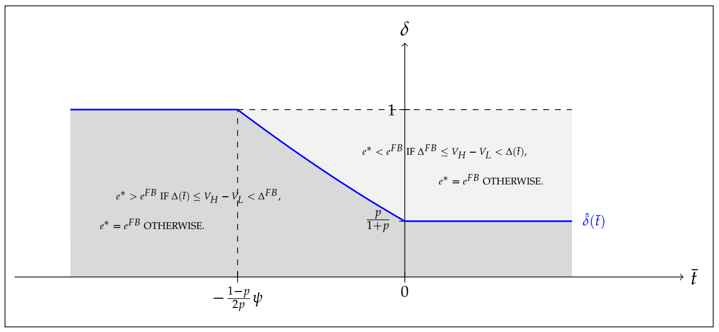
Lemma 1.

Suppose Assumption 1 holds. Then $\Delta \left(\overline{t}\right)⋚{\Delta }^{FB}$ if and only if $\delta ⋚\widehat{\delta }\left(\overline{t}\right)$, where

$$\begin{array}{c}\hfill \widehat{\delta }\left(\overline{t}\right):= \left\{\begin{array}{cc}\frac{p}{1+p}\hfill & \mathrm{if}0\le \overline{t},\hfill \\ \frac{p\left\{-[\psi (1+3p)+2\overline{t}(1+p)]+\sqrt{{\psi }^2{(p+3)}^2-4\overline{t}\psi (1-p^2)+4{\overline{t}}^2{(1+p)}^2}\right\}}{2\psi (1-p^2)}\hfill & \mathrm{if}{t}_L^{ST}\le \overline{t}<0,\hfill \\ 1\hfill & \mathrm{if}\overline{t}<t_L^{ST}\hfill \end{array}\right.\end{array}$$

(16)

is a continuous and weakly decreasing function.

The function $\widehat{\delta }(·)$ is depicted in Figure 5. Given liability level $\overline{t}$, whenever $\delta \ne \widehat{\delta }\left(\overline{t}\right)$, there is scope for the second-best effort level to diverge from the first-best effort level.

Proposition 4.

Suppose Assumption 1 holds. If $\delta <\widehat{\delta }\left(\overline{t}\right)$ and $\Delta \left(\overline{t}\right)\le V_H-V_L<{\Delta }^{FB}$, then the principal induces overwork (i.e., $e^{\ast }>e^{FB}$). If $\delta >\widehat{\delta }\left(\overline{t}\right)$ and ${\Delta }^{FB}\le V_H-V_L<\Delta \left(\overline{t}\right)$, then the principal induces underwork (i.e., $e^{\ast }<e^{FB}$). Otherwise the principal induces the first-best effort (i.e., $e^{\ast }=e^{FB}$).

If A’s salience bias is sufficiently weak, $\delta >\widehat{\delta }\left(\overline{t}\right)$, then, as in the standard model, any distortion away from the first-best effort results in underwork. In contrast to the standard model, however, if A’s salience bias is sufficiently strong, $\delta >\widehat{\delta }\left(\overline{t}\right)$, then the inefficient effort provision takes the form of overwork. Notably, if $\overline{t}\le -\frac{p_3}{p_2}\psi =-\frac{1-p}{2p}\psi$, then $\widehat{\delta }\left(\overline{t}\right)=1$ such that P always induces the first-best effort in the standard model, even a small degree of salience bias opens the door for overwork to prevail.

These observations are summarized in Figure 5. Note that the results of the standard model are also contained in this figure, which can be seen by looking at the dashed horizontal line at $\delta =1$.

Proposition 4 relates the effort level, $e^{\ast }$, induced under the optimal contract for a salience-biased agent at Benchmark 1, i.e., to the materially efficient effort level $e^{FB}$. Next, we want to compare $e^{\ast }$ to Benchmark 2, i.e., to the effort level, $\tilde{e}$, induced under the optimal contract for an unbiased agent. One can verify that $\frac{d\Delta \left(\overline{t}\right)}{d\delta }>0$, which implies that $\tilde{\Delta }>\Delta \left(\overline{t}\right)$ for all $\delta \in (0,1)$ and $\overline{t}\in \mathbb{R}$. As a consequence, $\tilde{e}\le e^{\ast }$ for all $\delta \in (0,1)$ and $\overline{t}\in \mathbb{R}$. Hence, if the principal faces an agent whose perception is blurred by salience bias, she always induces weakly, and in some circumstances strictly, higher effort than in the case where she faces an unbiased agent who perceives the occurrence probabilities correctly. Specifically, if $\tilde{e}=e^{FB}<e^{\ast }$, then salience bias is detrimental for material efficiency as it induces overwork, which is never the result for an unbiased agent. If, in contrast, $\tilde{e}<e^{FB}=e^{\ast }$, then salience bias fosters material efficiency as underwork would prevail in the case of an unbiased agent.

To conclude, let us entertain a thought experiment that might help to understand why employees may actually feel overworked, as found by Galinsky et al. [22]. At first glance, this observation seems at odds with our model, given that a salience-biased agent also considers his decision to accept a contract and his decision to exert high effort as utility maximizing at the moment when he makes the respective decision. Imagine that a salience-biased agent accepted a contract under which he exerts high effort, i.e., under which $e^{\ast }=1$. As we know from Proposition 1, under this contract either the incentive compatibility constraint binds and the participation constraint is slack (if $\overline{t}>t_L^{ST}$), or the participation constraint binds and the incentive compatibility constraint is slack (if $\overline{t}<t_L^{ST}$). Suppose that we can slightly reduce the degree of the agent’s salience bias right before these decisions. Irrespective of which constraint was binding in the presence of salience bias, the respective constraint is violated for the lower degree of salience bias. That is to say, if the incentive compatibility constraint is binding in the presence of salience bias, then, once we weaken the bias, the agent would agree that he had almost accidentally exerted more effort than is good for him. Likewise, if the participation constraint is binding in the presence of salience bias, then, once we weaken the bias, the agent would agree that he almost accidentally entered into a work relationship even though he is better off rejecting the principal’s contract offer. While it may not be possible for us to reduce the degree of the agent’s salience bias at will, one might imagine that the salience-blurred perception, which shapes a particular decision will fade out once the decision has been taken and the agent’s attention is shifted elsewhere. In this case, it stands to reason that the agent, in retrospect, will realize that he has overextended himself in the past by exerting more effort on a task than he now deems worthwhile or by agreeing to take on the task in the first place.

4. Discussion

In this paper, we enriched an otherwise standard principal–agent model of moral hazard with hidden action by salience-biased perception [25] on the agent’s side and analyzed its implications for incentive provision. In comparison to the standard model, we found that salience bias can reverse the nature of the inefficiency that arises from the agent being privately informed about his own work effort, i.e., the principal does not necessarily provide insufficient incentives that result in inefficiently low effort, but instead may provide excessive incentives that result in inefficiently high effort. The reason overwork may prevail is that the agent’s misguided focus on salient payoffs facilitates incentive provision and allows the principal to exploit diverging prior beliefs to her advantage.

The first immediately related question is to what extent this finding is specific to the model of salience theory for choice under risk outlined by Bordalo et al. [25]. As the result is rooted in the excess weight or excess attention that is placed on states with rather different payoffs, any state-space based theory that embodies the psychological principle of similarity judgments [52,53] in one way or the other should yield qualitatively similar results.15 The advantage of salience theory is its tractability, because, even if the agent’s remuneration is contingent on his performance (i.e., even if the transfer paid in case of generation of high value is strictly different from the transfer paid in case of generation of low value), the distortion in the decision weights does not depend on the specifics of the contractually specified transfer payments, and the contracting problem remains a simple linear programming problem.

A second related question is whether our study allows us to identify ways to deal with overwork as a social problem. An obvious answer would be to reduce salience bias by training the agent (e.g., a worker or a manager) in his assessment of stochastic processes. The adequacy of this solution is, however, open to question. First, inferential errors are commonly regarded as errors of application [57], i.e., individuals alerted to an error in judgment in one instance seem unable to avoid making the very same error in subsequent judgments. Thus, awareness training is arguably not a fail-safe device to cope with overwork. Second, the principal has no incentive to incur the cost for implementing such awareness training for the agent, because her expected utility increases with the severity of salience bias (cf. Corollaries 1 and 2). Hence, coping with overwork seems to call for regulatory intervention. A practical approach suggested by our analysis is the imposition of a sufficiently high minimum wage. As can be seen from Figure 5, the severity of salience bias necessary for overwork to possibly prevail is highest if transfers from the principal to the agent cannot be negative. In fact, with $\widehat{\delta }\left(\overline{t}\right)<\frac{1}{2}$ for $\overline{t}>0$, the estimation in Königsheim et al. [45], who estimate the salience parameter $\delta$ to equal 0.7–0.8, suggests that overwork should not arise in the presence of a non-negative minimum wage.16

Throughout our analysis, we assumed that the agent’s outside option has no effect on his salience-blurred perception of the occurrence probabilities of the different monetary outcomes feasible under the principal’s contract offer. As noted before, this assumption seems reasonable if the reservation utility associated with A’s outside option has a non-monetary origin such as the stigma or the shame of being unemployed. However, one might also imagine that, if the agent’s outside option is unemployment, his reservation utility is primarily tied to monetary unemployment benefits. As monetary unemployment benefits can rather easily be compared to the monetary transfer payments specified in the principal’s contract offer, they might affect salience. Extending our model in this regard would allow us to address the heretofore unexplored participation and incentive effects of unemployment benefits, which, we believe, is a highly interesting and policy-relevant venue for future research.

References

- Hart, O.; Holmstrom, B. The Theory of Contracts. In Advances in Economics and Econometrics, Econometric Society Monographs, Fifth World Congress; Bewely, T., Ed.; Camebridge University Press: Camebridge, UK, 1987; pp. 71–155. [Google Scholar]
- Innes, R.D. Limited Liability and Incentive Contracting with Ex-Ante Action Choices. J. Econ. Theory 1990, 52, 45–67. [Google Scholar] [CrossRef]
- Baliga, S.; Sjöström, T. Decentralization and Collusion. J. Econ. Theory 1998, 83, 196–232. [Google Scholar] [CrossRef] [Green Version]
- Pitchford, R. Moral Hazard and Limited Liability: The Real Effects of Contract Bargaining. Econ. Lett. 1998, 61, 251–259. [Google Scholar] [CrossRef] [Green Version]
- Berkovitch, E.; Israel, R.; Spiegel, Y. A Double Moral Hazard Model of Organization Design. J. Econ. Manag. Strategy 2010, 19, 55–85. [Google Scholar] [CrossRef]
- Kaya, A.; Vereshchagina, G. Partnerships versus Corporations: Moral Hazard, Sorting, and Ownership Structure. Am. Econ. Rev. 2001, 104, 291–307. [Google Scholar] [CrossRef] [Green Version]
- Dai, T.; Jerath, K. Salesforce Compensation with Inventory Considerations. Manag. Sci. 2013, 59, 2490–2501. [Google Scholar] [CrossRef]
- Kräkel, M.; Schöttner, A. Optimal Sales Force Compensation. J. Econ. Behav. Organ. 2016, 126, 179–195. [Google Scholar] [CrossRef] [Green Version]
- Schöttner, A. Optimal Sales Force Compensation in Dynamic Settings: Commissions vs. Bonuses. Manag. Sci. 2017, 63, 1529–1544. [Google Scholar] [CrossRef] [Green Version]
- Schmitz, P.W. Allocating Control in Agency Problems with Limited Liability and Sequential Hidden Actions. RAND J. Econ. 2005, 36, 318–336. [Google Scholar]
- Hoppe, E.I.; Kusterer, D.J. Conflicting Tasks and Moral Hazard: Theory and Experimental Evidence. Eur. Econ. Rev. 2011, 55, 1094–1108. [Google Scholar] [CrossRef]
- Kragl, J.; Schöttner, A. Wage Floors, Imperfect Performance Measures, and Optimal Job Design. Int. Econ. Rev. 2014, 55, 525–550. [Google Scholar] [CrossRef] [Green Version]
- Pi, J. Job Design with Sequential Tasks and Outcome Externalities Revisited. Econ. Lett. 2014, 125, 274–277. [Google Scholar] [CrossRef]
- Pi, J. Another Look at Job Design with Conflicting Tasks. Aust. Econ. Pap. 2018, 57, 427–434. [Google Scholar] [CrossRef]
- Che, Y.K.; Yoo, S.W. Optimal Incentives for Teams. Am. Econ. Rev. 2001, 93, 525–541. [Google Scholar] [CrossRef] [Green Version]
- Tamada, Y.; Tsai, T.S. Delegating the Decision-Making Authority to Terminate a Sequential Project. J. Econ. Behav. Organ. 2014, 99, 178–194. [Google Scholar] [CrossRef]
- Kräkel, M.; Schöttner, A. Delegating Pricing Authority to Sales Agents: The Impact of Kickbacks. Manag. Sci. 2019, 66, 2686–2705. [Google Scholar] [CrossRef]
- At, C.; Friehe, T.; Gabuthy, Y. On Lawyer Compensation when Appeals are Possible. BE J. Econ. Anal. Policy 2019, 19, 1–11. [Google Scholar] [CrossRef]
- Schmitz, P.W. Workplace Surveillance, Privacy Protection, and Efficiency Wages. Labour Econ. 2005, 12, 727–738. [Google Scholar] [CrossRef] [Green Version]
- Nieken, P.; Schmitz, P.W. Repeated Moral Hazard and Contracts with Memory: A Laboratory Experiment. Games Econ. Behav. 2012, 75, 1000–1008. [Google Scholar] [CrossRef] [Green Version]
- Hoppe, E.I.; Schmitz, P.W. Hidden Action and Outcome Contractibility: An Experimental Test of Moral Hazard Theory. Games Econ. Behav. 2018, 109, 544–564. [Google Scholar] [CrossRef]
- Galinsky, E.; Bond, J.T.; Kim, S.; Backon, L.; Brownfield, E.; Sakai, K. Overwork in America: When the Way We Work Becomes Too Much; Families and Work Institute: New York, NY, USA, 2005. [Google Scholar]
- Harnois, G.; Gabriel, P. Mental Health and Work: Impact, Issues and Good Practices; World Health Organization and International Labour Organisation: Geneva, Switzerland, 2000; WHO/MSD/MPS/00.2. [Google Scholar]
- Galinsky, E. Ask the Children: What America’s Children Really Think about Working Parents; William Morrow and Company, Inc.: New York, NY, USA, 1999. [Google Scholar]
- Bordalo, P.; Gennaioli, N.; Shleifer, A. Salience Theory for Choice under Risk. Q. J. Econ. 2012, 127, 1243–1285. [Google Scholar] [CrossRef] [Green Version]
- Kontek, K. A Critical Note on Salience Theory of Choice under Risk. Econ. Lett. 2016, 143, 168–171. [Google Scholar] [CrossRef]
- Bako, B.; Neszveda, G. The Achilles’ Heel of Salience Theory and How to Fix It. Econ. Lett. 2020, 193, 109265. [Google Scholar] [CrossRef]
- Holmström, B. Moral Hazard and Observability. Bell J. Econ. 1979, 10, 74–91. [Google Scholar] [CrossRef] [Green Version]
- Grossman, S.J.; Hart, O.D. An Analysis of the principal–agent Problem. Econometrica 1983, 51, 7–46. [Google Scholar] [CrossRef] [Green Version]
- Kräkel, M.; Schöttner, A. Minimum Wages and Excessive Labor Supply. Econ. Lett. 2010, 108, 341–344. [Google Scholar] [CrossRef] [Green Version]
- Ohlendorf, S.; Schmitz, P.W. Repeated Moral Hazard and Contracts with Memory: The Case of Risk-Neutrality. Int. Econ. Rev. 2012, 53, 433–452. [Google Scholar] [CrossRef] [Green Version]
- Englmaier, F.; Fahn, M.; Schwarz, M.A. Long-Term Employment Relations When Agents Are Present Biased; CEPR Discussion Paper No. DP13227; 2018; Available online: https://econpapers.repec.org/paper/cprceprdp/13227.htm (accessed on 6 December 2021).
- Goldlücke, S.; Schmitz, P.W. Pollution Claim Settlements Reconsidered: Hidden Information and Bounded Payments. Eur. Econ. Rev. 2018, 110, 211–222. [Google Scholar] [CrossRef]
- Bordalo, P.; Gennaioli, N.; Shleifer, A. Salience and Consumer Choice. J. Political Econ. 2013, 127, 803–843. [Google Scholar] [CrossRef] [Green Version]
- Herweg, F.; Müller, D.; Weinschenk, P. Salience in Markets. In Handbook of Behavioral Industrial Organization; Edward Elgar Publishing: Cheltenham, UK, 2018. [Google Scholar]
- Adrian, N. Price Discrimination and Salience-Driven Consumer Preferences; Technical Report, Discussion Papers; University of Bern: Bern, Switzerland, 2019. [Google Scholar]
- Friehe, T.; Pham, C.L. Settling with Salience-biased Defendants. Econ. Lett. 2020, 192, 109235. [Google Scholar] [CrossRef]
- Mungan, M.C. Salience and the Severity versus the Certainty of Punishment. Int. Rev. Law Econ. 2019, 57, 96–100. [Google Scholar] [CrossRef]
- de la Rosa, L.E. Overconfidence and Moral Hazard. Games Econ. Behav. 2011, 73, 429–451. [Google Scholar] [CrossRef] [Green Version]
- Müller, D.; Schmitz, P.W. The Right to Quit Work: An Efficiency Rationale for Restricting the Freedom of Contract. J. Econ. Behav. Organ. 2021, 184, 653–669. [Google Scholar] [CrossRef]
- Laffont, J.J.; Martimort, D. The Theory of Incentives: The Principal–Agent Model; Princeton University Press: Princeton, NJ, USA, 2002. [Google Scholar]
- Salanié, B. The Economics of Contracts: A Primer; MIT Press: Cambridge, MA, USA, 2005. [Google Scholar]
- Bordalo, P.; Gennaioli, N.; Shleifer, A. Salience and Asset Prices. Am. Econ. Rev. Pap. Proc. 2013, 103, 623–628. [Google Scholar] [CrossRef] [Green Version]
- Cosemans, M.; Frehen, R. Salience Theory and Stock Prices: Empirical Evidence. J. Financ. Econ. 2021, 140, 460–483. [Google Scholar] [CrossRef]
- Königsheim, C.; Lukas, M.; Nöth, M. Salience Theory: Calibration and Heterogeneity in Probability Distortion. J. Econ. Behav. Organ. 2019, 157, 477–495. [Google Scholar] [CrossRef]
- Alós-Ferrer, C.; Ritschel, A. Attention and Salience in Preference Reversals. Exp. Econ. 2022. [Google Scholar] [CrossRef]
- Sandroni, A.; Squintani, F. Overconfidence, Insurance, and Paternalism. Am. Econ. Rev. 2007, 97, 617–622. [Google Scholar] [CrossRef] [Green Version]
- Grubb, M. Selling to Overconfident Consumers. Am. Econ. Rev. 2009, 99, 1770–1807. [Google Scholar] [CrossRef] [Green Version]
- Herweg, F.; Müller, D. Overconfidence in the Markets for Lemons. Scand. J. Econ. 2016, 118, 354–371. [Google Scholar] [CrossRef] [Green Version]
- Eliaz, K.; Spiegler, R. Contracting with Diversely Naive Agents. Rev. Econ. Stud. 2006, 73, 689–714. [Google Scholar] [CrossRef]
- Eliaz, K.; Spiegler, R. Consumer Optimism and Price Discrimination. Theor. Econ. 2008, 3, 459–497. [Google Scholar]
- Luce, R.D. Individual Choice Behavior: A Theoretical Analysis; Wiley: New York, NY, USA, 1959. [Google Scholar]
- Tversky, A. Features of Similarity. Psychol. Rev. 1977, 84, 327. [Google Scholar] [CrossRef]
- Loomes, G.; Sugden, R. Regret Theory: An Alternative Theory of Rational Choice under Uncertainty. Econ. J. 1982, 92, 805–824. [Google Scholar] [CrossRef]
- Kőszegi, B.; Szeidl, A. A Model of Focusing in Economic Choice. Q. J. Econ. 2013, 128, 53–104. [Google Scholar] [CrossRef]
- Bhatia, S.; Loomes, G.; Read, D. Establishing the Laws of Preferential Choice Behavior. Judgm. Decis. Mak. 2021, 16, 1324–1369. [Google Scholar]
- Kahneman, D.; Tversky, A. On the Study of Statistical Intuitions. Cognition 1982, 11, 123–141. [Google Scholar] [CrossRef]
Figure 1.
and .
Figure 2.
Figure 3.
Figure 4.
Figure 5.
Second-best effort.