Ex Post Nash Equilibrium in Linear Bayesian Games for Decision Making in Multi-Environments

Abstract

We show that a Bayesian game where the type space of each agent is a bounded set of m-dimensional vectors with non-negative components and the utility of each agent depends linearly on its own type only is equivalent to a simultaneous competition in m basic games which is called a uniform multigame. The type space of each agent can be normalised to be given by the $(m-1)$-dimensional simplex. This class of m-dimensional Bayesian games, via their equivalence with uniform multigames, can model decision making in multi-environments in a variety of circumstances, including decision making in multi-markets and decision making when there are both material and social utilities for agents as in the Prisoner’s Dilemma and the Trust Game. We show that, if a uniform multigame in which the action set of each agent consists of one Nash equilibrium inducing action per basic game has a pure ex post Nash equilibrium on the boundary of its type profile space, then it has a pure ex post Nash equilibrium on the whole type profile space. We then develop an algorithm, linear in the number of types of the agents in such a multigame, which tests if a pure ex post Nash equilibrium on the vertices of the type profile space can be extended to a pure ex post Nash equilibrium on the boundary of its type profile space in which case we obtain a pure ex post Nash equilibrium for the multigame.

1. Introduction

In this paper, we study linear multidimensional Bayesian games in which the type of each agent is a finite dimensional real vector and the utility of each agent only depends linearly on its own type. Multidimensional Bayesian games have been studied by Krishna and Perry in the context of multiple object auctions whose utilities are piecewise affine maps of the types of the agents [1]. This class includes all combinatorial auction problems (see [2,3] and [4] (Chapter 7)). The challenge posed by multidimensional private information is that multidimensional type spaces can be large and may be analytically or computationally intractable [3]. In [5], Bayesian games with multidimensional types where a utility of an agent depends only on the actions performed by others and not on their type and each agent draws its type independently from a commonly known continuous distribution have been studied.

We show that a multidimensional linear Bayesian game where the type space of each agent is a bounded set of m-dimensional vectors, with non-negative components, is equivalent to a simultaneous competition in m basic games, called a uniform multigame, as introduced in [6,7], in which the utility of each agent only depends linearly on its own type and each agent plays the same strategy in all basic games. While this equivalent representation provides no reduction in the size of input parameters, i.e., it is not more concise, it does establish a new and, we argue, conceptually useful representation of the multidimensional Bayesian game. In fact, using their equivalence with multigames, this class of multidimensional Bayesian games can model the common situation in which a number of agents allocate their resources or investment to several independent environments or basic games. The type space of each agent can be normalised to coincide with the $(m-1)$-dimensional simplex in ${\mathbb{R}}^m$. Then, the amount of investment of agents in each environment would be replaced with their investment rate in that environment, and the total utility would amount to the convex combination of the individual utility for each environment weighted by the rate of investment or type for that environment.

We seek an appropriate notion of equilibrium for this class of Bayesian games. Recall that the key concept of Pareto efficiency can be used to evaluate the performance of various systems including in an economy [8]. Holmstrom and Myerson suggested three evaluation stages: ex ante, before the agents have received any private information; interim, when each agent has received its private information, but does not know the other’s information; and ex post, when the information is public knowledge [9]. In [10], ex post Nash equilibrium (NE) is employed to deal with the optimal design of mechanisms of resource allocations. Bergemann and Morris justified employing ex post NE as a solution concept in which no agent would have an incentive to change its strategy even if it were to be informed of the true type profile of the other agents; a related justification for ex post NE, discussed by the same authors, is the distinguished feature of lack of regret in this type of equilibrium, which does not hold for Bayesian NE in general [11].

We propose that the solution concept of ex post NE is also a useful tool for multigames in general and for uniform multigames in particular and thus for the class of linear multidimensional Bayesian games as discussed above. We first actually show the simple result that for a multigame, a pure ex post NE can be obtained in constant time if a set of pure NE for all the basic games is already given. In fact, the ex post NE in this context is simply provided by the strategy profile where each agent for any basic game takes, in each environment, the action specified for that agent by the NE strategy profile for that environment. In the rest of the paper, we focus on finding a pure ex post NE for a class of uniform multigames, called standard uniform multigames, commonly encountered in many applications, where each agent plays uniformly in all games by choosing one action from an action set consisting of a NE inducing action per game.

We extend the concept of ex post NE, which is usually defined on the product of the agents’ type spaces, to any subset of type profile space and establish that a standard uniform multigame has an ex post NE, compatible with the standard structure, if its restriction to the boundary of its type profile space has an ex post NE. We then derive an algorithm, linear in the number of types of the agents, which checks, for a standard uniform multigame with n agents and m basic games, if a pure ex post NE on the vertices of the type profile space extends to a pure ex post NE on its boundary, in which case we obtain a pure ex post NE for the multigame. We present an outline of the main sections of the paper after deriving some simple properties of ex post NE in Section 2 which also gives the motivation for our key results.

1.1. Comparison with Related Work

As in multigames, in networked Cournot competition, agents play simultaneously in more than one game. In [12], Bulow et al. provided a numerical example of Cournot markets in which two firms sell in one market and one of them is a monopolist in a second market. More recently, several authors have examined a network approach to Cournot competition [13,14] which gives an example of simultaneous competition. In this approach, a bipartite graph determines which subset of markets a given firm can supply to. Thus, the aim in [13] is to derive algorithms that compute the pure strategy Nash equilibria, while the work in [14] provides characterisations of equilibrium production quantities and studies the impact of changes in the competition structure such as expansion to a new market and merger of companies.

Multi-games have some similarities and yet some basic differences with polymatrix games [15], one of several well-studied classes of compactly represented games, which also include graphical games [16], hypergraphical game [17], and graphical multi-hypermatrix games [18]. Recall that a two-agent Bayesian game with a finite number of types can be represented by a polymatrix game [19]. In a polymatrix game, every agent plays the same strategy in every two-agent subgame, and its utility is the sum of its subgame utilities. In a multigame, however, the utility of each agent for any strategy profile in any local game, i.e, for any type profile, is a weighted sum of its n-agent basic game utilities where the weights, considered as private information, are given by the components of the agent’s type.

We note that, in general, the complexity of computing even an approximate pure Bayesian NE in Bayesian games has been shown to be NP-hard [20]. For two-agent Bayesian games with a finite number of types which can be represented by polymatrix games, Rubinstein proved that there exists a small $ϵ>0$ such that finding an $ϵ$-approximate NE is PPAD-complete [21]. In the case of Bayesian games considered in this paper, due to the exponential size of the type profile set in the expanded, i.e., extensive, game, the computation of an ex post NE of a uniform multigame, equivalently a linear multidimensional Bayesian game, is intractable even if the number of agents and basic games are small. The multigame representation of a linear multidimensional Bayesian game enables us, as described above, to develop an efficient algorithm to decide if a standard uniform multigame has a compatible ex post NE in which case the ex post NE is computed in constant time.

1.2. Applications of Multigames

In economics, multigames would, for example, arise when several companies divide up and allocate their funds to invest in different independent markets, e.g., US, EU and China, where each market has its own rate of return or utility. Companies generally are unaware of the amount of investment their rivals make and thus these can be considered as private information, yet the rate of return or utility in each market would depend on the amount the companies invest therein. Standard uniform multigames can be used to model economic behaviour in multi-environments in different contexts. They commonly arise, for example, when companies working in different markets consider whether to adopt a new technology. They can also be employed to model the situation in which several companies compete in m markets for the production and sale of $k\le m$ products where in each market one of these k products is optimal.

Similarly, multigames can arise in multiagent systems. When agents interact in a network, an agent can divide its resources such as time and allocate different portions of it to engage with other agents as in friendship networks [22]. If their resources are actually allocated to engage in different network games, we have a multigame.

Social Interactions and Sub-Personalities of Agents

In a completely different setting, standard uniform multigames can model decision making when both material and social utilities are involved. In recent years, a growing number of leading researchers in different disciplines have highlighted that decision making also has social and emotional components. In many situations, rational agents do not seem to behave in their self-interest, but rather behave pro-socially. In the past quarter of a century, various findings in neuroscience have also established that decision making has a significant and substantial emotional component which has to be taken into account together with its more cognitive and rational component (see [23,24,25] for a more in-depth discussion of this issue).

Gintis [26] (page xiv) argued that “humans have a social epistemology, meaning that we have reasoning processes that afford us forms of knowledge and understanding, especially the understanding and sharing of the content our minds, that are unavailable to merely ‘rational’ creatures. This social epistemology characterizes our species. The bounds of reason are thus not the irrational, but the social”. Gintis proposed a preference ordering in order to reflect individual beliefs and perceptions [26] (chapter 1).

A classic benchmark for modeling human decision making when self-interests are at stake is provided by the Prisoner’s Dilemma (PD) (see [27,28]). Housman [29] discussed the influence of social norms on decision making of individuals in the PD and observed that agents would not play the behaviour expected from the NE since the game theoretic model simplifies drastically the complexities of human mental life: “The Prisoner’s Dilemma shows that there are some institutional frameworks in which the self-interested choices of rational individuals are not socially beneficial”. This argument has been supported by several social experiments as in [30,31].

In the past two decades, the so-called Trust Game with two agents and an experimenter has been proposed to measure trust in human economic behaviour [32]. Initially, the two agents are given an equal amount of money. Then, in Stage 1, the first agent is asked to send some of its money to the experimenter who triples it and sends the tripled amount to the second agent. In Stage 2, the second agent is asked to send some of the money it has received by the experimenter to the first agent. The NE in the Trust Game stipulates that the first agent sends no money to the experimenter and the second agent also sends no money back to the first agent (see Section 7). However, in practice, human agents deviate from the NE as reported in experiments in [32,33] and also in a meta-analysis of 162 replications of the Trust Game involving more than 23,000 participants [34].

More generally, Davis [35] (Section 1.4) presented two broad domains on what is problematic with the traditional rationality theory as the basis of game theory. The first domain focuses on how we can interpret the effects of social interaction on rational agents’ choices. The second domain is how to account for the complex individuality or psychology of a rational agent which can be considered as different sub-personalities within the individual employing various empirical observations on making their strategies.

We propose that one way to redress the inadequacies of classical game theory and tackle the two problems raised by Davis [35] (Section 1.4), i.e., the social dimension of interaction between the agents and their sub-personalities in determining their strategies, is to use uniform multigames. This enables us for example in the PD or the Trust game to combine material and social utilities by allowing one environment, called the material game, to specify the material utilities and another environment, called the social game, to represent the social utilities. This provides an answer to the first problem, namely of social interaction, raised by Davis. In fact, since civilised societies generally commend collaboration and trust and censure defection and mistrust, the social game will have a NE when both agents collaborate, which counters the NE for the standard PD in which the NE occurs when both agents defect and the NE in the Trust Game when the two agents send each other zero money. The second problem, i.e., the sub-personalities of each agent, is addressed by the weights or types each agent allocates as private information to the material and the social game which indicate their materialistic and altruistic or trustful inclinations, respectively. We show in this paper that uniform multigames provide a more reasonable model of human behaviour in both the PD and the Trust Game. This, in particular, gives an alternative approach to that of Gintis [26] and that of Chaudhuri and Gangadharant [33] referred to above.

2. Bayesian Games and Their Ex Post NEs

We first recall the definition of a general class of Bayesian games as in [36] (p. 215). A Bayesian game G is a game in strategic form with incomplete information which has the following structure: $G=〈I,{(A_i,{\mathsf{\Theta }}_i,U_i)}_{i\in I},p(·)〉$ where $I=\{1,\dots ,n\}$ is the set of agents, $A_i$ is agent i’s action set, ${\mathsf{\Theta }}_i$ is agent i’s type space, and $U_i:{\prod }_{i\in I}{A}_i\times {\prod }_{i\in I}{\mathsf{\Theta }}_i\to \mathbb{R}$ is agent i’s utility for each $i\in I$. The agents’ type profile $({\theta }_1,\dots ,{\theta }_n)\in {\prod }_{i\in I}{\mathsf{\Theta }}_i$ is drawn from a given joint probability distribution $p({\theta }_1,\dots ,{\theta }_n)$. For any ${\theta }_i\in {\mathsf{\Theta }}_i$, the function $p(·|{\theta }_i)$ specifies a conditional probability distribution over ${\mathsf{\Theta }}_{-i}$ representing what agent i believes about the types of the other agents if its own type were ${\theta }_i$.

The type profile space of the game is defined as $\mathsf{\Theta }:={\prod }_{i\in I}{\mathsf{\Theta }}_i$. The pure strategy map space for agent $i\in I$ is the set $S_i^{{\mathsf{\Theta }}_i}=\{s_i(·):{\mathsf{\Theta }}_i\to A_i\}$ so that ${\prod }_{i\in I}{S}_i^{{\mathsf{\Theta }}_i}$ represents the space of all strategy map profiles. Recall that a strategy map profile $(s_1(·),\dots ,s_n(·))$ is a pure Bayesian NE if for each agent $i\in I$ and $s_i^{\prime }(·)\in S_i^{{\mathsf{\Theta }}_i}$, we have $U_i\left(s_i(·),s_{-i}(·)\right)\ge U_i\left(s_i^{\prime }(·),s_{-i}(·)\right)$ [36] (p. 215). For discrete type spaces, this is equivalent to

$$s_i({\theta }_i)\in arg\underset{a_i\in A_i}{max}\sum _{{\theta }_{-i}\in {\mathsf{\Theta }}_i}p({\theta }_{-i}|{\theta }_i)U_i\left(a_i,s_{-i}({\theta }_{-i}),{\theta }_i,{\theta }_{-i}\right),$$

for each $i\in I$ and ${\theta }_i\in {\mathsf{\Theta }}_i$. Let $\Delta (A_i)=\left\{{\sigma }_i(·):A_i\to [0,1]:{\sum }_{a_i\in A_i}{\sigma }_i(a_i)=1\right\}$ be the set of mixed actions for agent $i\in I$. By considering the normal form [36] (p. 3) of G, the mixed strategy map space for G is $\left\{{\sigma }_i(·):{\mathsf{\Theta }}_i\to \Delta (A_i)\right\}$. The notion of mixed Bayesian NE is defined similar to pure Bayesian NE.

In general, any Bayesian NE in games with incomplete information requires the prior distribution to be common knowledge. In many cases, however, the prior distribution may not be known, a situation that for example can occur in mechanism design [4,37,38]. In these cases, it is therefore desirable to relax this assumption. In fact, the necessary and sufficient condition for a Bayesian NE to be prior independent is that it be an ex post NE, which we now formally define.

Definition 1.

[10] Let G be a Bayesian game. A mixed strategy map profile $\left({\sigma }_1(·),\dots ,{\sigma }_n(·)\right)$ is an ex post NE if $U_i({\sigma }_i({\theta }_i),{\sigma }_{-i}({\theta }_{-i}),{\theta }_i,{\theta }_{-i})\ge U_i(a_i,{\sigma }_{-i}({\theta }_{-i}),{\theta }_i,{\theta }_{-i})$ for all $i\in I,({\theta }_i,{\theta }_{-i})\in {\mathsf{\Theta }}_i\times {\mathsf{\Theta }}_{-i},a_i\in A_i$.

Proposition 1.

Given a Bayesian game G, the strategy map profile $({\sigma }_1(·),\dots ,{\sigma }_n(·))$ is a Bayesian NE for all priors if and only if $({\sigma }_1(·),\dots ,{\sigma }_n(·))$ is an ex post NE.

Proof. 

It follows immediately from Definition 1 that, if in a Bayesian game the strategy map profile $\left({\sigma }_1(·),\dots ,{\sigma }_n(·)\right)$ is an ex post NE, then it is a Bayesian NE for all priors. Now, assume $({\sigma }_1(·),\dots ,{\sigma }_n(·))$ is a Bayesian NE for all prior p. We present the proof for the case when all agents have finite type spaces. The case of infinite type spaces, which uses integrals instead of sums to evaluate the utilities, is entirely similar. Hence, for each $i\in I$ and for any given ${\theta }_i\in {\mathsf{\Theta }}_i$, we have

$$\begin{array}{c}\hfill \sum _{{\theta }_{-i}^{\prime }\in {\mathsf{\Theta }}_{-i}}p({\theta }_{-i}^{\prime }|{\theta }_i)U_i({\sigma }_i({\theta }_i),{\sigma }_{-i}({\theta }_{-i}^{\prime }),{\theta }_i,{\theta }_{-i}^{\prime })\ge \sum _{{\theta }_{-i}^{\prime }\in {\mathsf{\Theta }}_{-i}}p({\theta }_{-i}^{\prime }|{\theta }_i)U_i(a_i,{\sigma }_{-i}({\theta }_{-i}^{\prime }),{\theta }_i,{\theta }_{-i}^{\prime })\end{array}$$

(1)

for each $a_i\in A_i$ and all priors p. For any given ${\theta }_{-i}\in {\mathsf{\Theta }}_{-i}$, define the conditional probability distribution: $p({\theta }_{-i}^{\prime }|{\theta }_i)=1$ if ${\theta }_{-i}^{\prime }={\theta }_{-i}$ and 0 otherwise. Using this prior p in Inequality (1), we deduce that $U_i({\sigma }_i({\theta }_i),{\sigma }_{-i}({\theta }_{-i}),{\theta }_i,{\theta }_{-i})\ge U_i(a_i,{\sigma }_{-i}({\theta }_{-i}),{\theta }_i,{\theta }_{-i})$ for each $a_i\in A_i$. Thus, the strategy map profile $({\sigma }_i(·),{\sigma }_{-i}(·))$ is an ex post NE for G. □

Definition 2.

The restriction of a Bayesian game G to a given type profile $({\theta }_1,\dots ,{\theta }_n)\in \mathsf{\Theta }$ is denoted by $G_{({\theta }_1,\dots ,{\theta }_n)}$ and is called the local game for G at $({\theta }_1,\dots ,{\theta }_n)$.

For formulating the results of this paper, we need to extend the notion of ex post NE, which is usually defined on the product of the agents’ type spaces as in Definition 1, to an arbitrary subset of the type profile space. Let the projection map ${\pi }_i:{\prod }_{i\in I}{\mathsf{\Theta }}_i\to {\mathsf{\Theta }}_i$, for each $i\in I$, be given by ${\pi }_i({\theta }_1,\dots ,{\theta }_n)={\theta }_i$. Let $f\left[B\right]$ denote the forward image of map f on the subset B.

Definition 3.

A Bayesian game G has an ex post NE on ${\mathsf{\Theta }}^{\prime }\subseteq \mathsf{\Theta }$ if for each agent $i\in I$ there exists a function ${\sigma }_i(·):{\pi }_i[{\mathsf{\Theta }}^{\prime }]\to \Delta (A_i)$ such that the strategy profile $\left({\sigma }_1({\theta }_1),\dots ,{\sigma }_n({\theta }_n)\right)$ is a NE for the local game $G_{({\theta }_1,\dots ,{\theta }_n)}$ whenever $({\theta }_1,\dots ,{\theta }_n)\in {\mathsf{\Theta }}^{\prime }$.

In other words, Definition 3 means that a Bayesian game G has an ex post NE on ${\mathsf{\Theta }}^{\prime }$ if for each agent and a given type for it from an element of the set ${\mathsf{\Theta }}^{\prime }$, the agent can select an action dependent only on the given type, such that for each type profile of all agents in ${\mathsf{\Theta }}^{\prime }$ the resulting action profile is a NE for the local game specified by that type profile. Clearly, Definition 3 is an extension of Definition 1. Note from Definition 1 that, if G has a pure ex post NE, then it has a pure ex post NE on any subset of ${\mathsf{\Theta }}^{\prime }\subseteq \mathsf{\Theta }$.

The following property is directly obtained from Definition 1:

Proposition 2.

An ex post NE of a Bayesian game induces a NE for each local game.

Outline of the Paper

One way to interpret the quest for the main results of this paper and to motivate the next sections is to say that we seek a finitary converse to Proposition 2, i.e., find a simple but general class of Bayesian games for which we can obtain a pure ex post NE by representing the agents’ interactions in the Bayesian game with a finite number of its local games, considered as basic games, and by using a given set of NE inducing pure strategies one per such basic game.

With this aim in mind, we can explain the rest of the paper as follows. In Section 3, we show that a linear multidimensional Bayesian game, i.e., one in which the type space of each agent is a bounded subset of ${\mathbb{R}}_{+}^m$ for some positive integer m and the utility of each agent for each strategy depends only linearly on its own type components, can be represented as a simultaneous competition of the agents in m local games. We formulate an intrinsic definition for a more general version of such simultaneous competitions called multigames which have a simple pure ex post NE induced by a set of NE of its basic games. We then verify in this section that linear multidimensional Bayesian games are equivalent with uniform multigames in which each agent plays the same strategy in all basic games.

In Section 4, we introduce the notion of a standard uniform multigame, which incorporates a set of NE inducing pure strategies one per basic game. This provides a simple but general class of Bayesian games in which the analysis of a pure ex post NE can be reduced, as stipulated above, to a set of NE in a finite number of its local games. We illustrate the framework by an extension of the PD with a social game which plays the role of a running example for the main results of the paper in the later sections.

We then show in Section 5 that, if a standard uniform multigame has a pure ex post NE, compatible with the standard structure, on the boundary of its type profile space, then it has a pure ex post NE on the whole type profile space. In addition, we develop an algorithm, linear in the number of types of the agents in a standard uniform multigame, which tests if a compatible pure ex post NE on the vertices of the type profile space can be extended to a pure ex post NE on the boundary of its type profile space in which case we obtain a pure ex post NE for the multigame. In Section 6, we present two applications of standard uniform multigames in multimarkets. In Section 7, we develop an extension of the Trust Game to a standard uniform double game in a multistage context.

3. Linear Multidimensional Bayesian Games and Uniform Multigames

In this section, we define the class of linear multidimensional Bayesian games and show that they are equivalent to simultaneous competitions in a finite number of basic games in which each agent plays the same action in all basic games.

Definition 4.

A Bayesian game G is m-dimensional if the type space of each agent is a bounded subset of ${\mathbb{R}}_{+}^m$. When the positive integer $m>1$ is implicitly given, we say G is multidimensional. A multidimensional Bayesian game is linear if the utility of each agent only depends linearly on its own type components, i.e., there exists $L_i(s_i,s_{-i})\in {\mathbb{R}}^m$ such that $U_i(s_i,s_{-i},{\theta }_i,{\theta }_{-i})={\sum }_{j\in J}{(L_i(s_i,s_{-i}))}_j{\theta }_{ij}$.

We show that a linear m-dimensional Bayesian game is equivalent to a simultaneous competition of its agents in m basic games. To make this precise, we define the notion of a multigame. A multigame, as a Bayesian game, models the behavior of a finite number of rational agents who play in a number of different environments simultaneously. Each environment is represented by a basic game and the resources of each agent are allocated with varying proportions, as private information, to these basic games.

Definition 5.

A multigame G is a game in strategic form with incomplete information

$$G=〈I,J,{\{w_i\}}_{i\in I},{\{G_j\}}_{j\in J},{\{{\mathsf{\Theta }}_i\}}_{i\in I},{\{A_{ij}\}}_{i\in I,j\in J},{\{U_{ij}\}}_{i\in I,j\in J},p(·)〉$$

which has the following structure:

1. 

The set of agents is $I=\{1,\dots ,n\}$.

2. 

The set of n-agent basic games is $G_j$, where $j\in J=\{1,\dots ,m\}$ with action space $A_{ij}$ and utility function $U_{ij}$ for each agent $i\in I$ in the game $G_j$.

3. 

Agent i’s strategy is $s_i=(s_{i1},\dots ,s_{im})\in S_i={\prod }_{j\in J}{A}_{ij}$ where $s_{ij}$ is agent i’s action in $G_j$.

4. 

Agent i’ type is ${\theta }_i=({\theta }_{i1},\dots ,{\theta }_{im})\in {\mathsf{\Theta }}_i$ with ${\theta }_{ij}\ge 0$, $w_i>0$ and ${\sum }_{j\in J}{\theta }_{ij}\le w_i$.

5. 

Agent i’s utility for the strategy profile $(s_i,s_{-i})$ and type profile $({\theta }_i,{\theta }_{-i})$ depends linearly on its types:

$$U_i(s_i,s_{-i},{\theta }_i,{\theta }_{-i})=\sum _{j\in J}{\theta }_{ij}{U}_{ij}(s_{1j},\dots ,s_{nj}).$$

6. 

The agents’ type profile $({\theta }_1,\dots ,{\theta }_n)\in {\prod }_{i\in I}{\mathsf{\Theta }}_i$ is drawn from a given joint probability distribution $p({\theta }_1,\dots ,{\theta }_n)$. For any ${\theta }_i\in {\mathsf{\Theta }}_i$, the function $p(·|{\theta }_i)$ specifies a conditional probability distribution over ${\mathsf{\Theta }}_{-i}$ representing what agent i believes about the types of the other agents if its own type were ${\theta }_i$.

Note that $w_i$ is an upper bound for the sum of investments of agent i in the basic games. We say that a multigame is normalised if for each agent $i\in I$, we have ${\sum }_{j\in J}{\theta }_{ij}=w_i=1$. By considering an additional game, we can always normalise a multigame as follows.

Proposition 3.

The multigame $G=〈I,J,{\{w_i\}}_{i\in I},{\{G_j\}}_{j\in J},{\{{\mathsf{\Theta }}_i\}}_{i\in I},{\{A_{ij}\}}_{i\in I,j\in J},{\{U_{ij}\}}_{i\in I,j\in J},p(·)〉$ is equivalent with $\widehat{G}=〈I,\widehat{J},{\{{\widehat{w}}_i\}}_{i\in I},{\{{\widehat{G}}_j\}}_{j\in \widehat{J}},{\{{\widehat{\mathsf{\Theta }}}_i\}}_{i\in I},{\{A_{ij}\}}_{i\in I,j\in J},{\{{\widehat{U}}_{ij}\}}_{i\in I,j\in J},p(·)〉$ having the following structure:

1. 

The set of n-agent basic games is ${\widehat{G}}_j$ where $\widehat{J}=J\cup \{m+1\}$ with: (i) action space $A_{ij}$ and utility function ${\widehat{U}}_{ij}$ for each agent $i\in I$ in the game ${\widehat{G}}_j$ with ${\widehat{U}}_{ij}=w_i{U}_{ij}$ for each $j\in J$; and (ii) action set $A_{i(m+1)}=A_{i1}$ and utility function ${\widehat{U}}_{i(m+1)}(s_{i(m+1)},s_{-i(m+1)})=0$ for each $s_{i(m+1)}\in A_{i(m+1)}$ and $s_{-i(m+1)}\in A_{-i(m+1)}$.

2. 

Agent i’s type space,

$${\widehat{\mathsf{\Theta }}}_i=\left\{\left(\frac{{\theta }_{i1}}{w_i},\dots ,\frac{{\theta }_{im}}{w_i},1-\frac{{\sum }_{j\in J}{\theta }_{im}}{w_i}\right)|({\theta }_{i1},\dots ,{\theta }_{im})\in {\mathsf{\Theta }}_i\right\}.$$

3. 

Agent i’s total resource is ${\widehat{w}}_i=1$.

Proof. 

Assume ${\widehat{\theta }}_i=\left({\theta }_{i1}/w_i,\dots ,{\theta }_{im}/w_i,1-{\sum }_{j\in J}{\theta }_{ij}/w_k\right)\in {\widehat{\mathsf{\Theta }}}_i$ where $i\in I$. For each agent $i\in I$ and $(s_i,s_{-i})\in S_i\times S_{-i}$, we have

$$\begin{array}{c}\hfill {\widehat{U}}_i(s_i,s_{-i},{\widehat{\theta }}_i,{\widehat{\theta }}_{-i})=\sum _{j\in \widehat{J}}{\widehat{\theta }}_{ij}{\widehat{U}}_{ij}(s_{ij},s_{-ij})=\sum _{j\in J}{\widehat{\theta }}_{ij}{\widehat{U}}_{ij}(s_{ij},s_{-ij})=\sum _{j\in J}\frac{{\theta }_{ij}}{w_i}(w_i{U}_{ij}(s_{ij},s_{-ij}))=U_i(s_i,s_{-i},{\theta }_i,{\theta }_{-i}),\end{array}$$

as required. □

The following simple result shows that a Bayesian NE for a multigame can be computed in constant time with respect to the number of types and independent of the prior probability distribution if a set of NEs for all its basic games is given.

Proposition 4.

Let G be a multigame and $(s_{1j},\dots ,s_{nj})$ a NE for its basic game $G_j$ with $j\in J$. Then, $(s_1(·),\dots ,s_n(·))$, where $s_i(·):{\mathsf{\Theta }}_i\to S_i$ is given by $s_i({\theta }_i)=(s_{i1},\dots ,s_{im})$, is an ex post NE.

Proof. 

Consider any strategy $s_i^{\prime }(·):{\mathsf{\Theta }}_i\to S_i$. By definition: $U_i(s_i\left({\theta }_i\right),s_{-i}\left({\theta }_{-i}\right),{\theta }_i,{\theta }_{-i})={\sum }_{j\in J}{\theta }_{ij}{U}_{ij}(s_{ij},s_{-ij}).$ Since $(s_{ij},s_{-ij})$ is a NE for $G_j$, $U_{ij}(s_{ij},s_{-ij})\ge U_{ij}(s_{ij}^{\prime },s_{-ij})$ for $j\in J$ where $s^{\prime }\left({\theta }_i\right)={(s_{ij}^{\prime })}_{j\in J}$. Therefore, $U_i(s_i({\theta }_i),s_{-i}({\theta }_{-i}),{\theta }_i,{\theta }_{-i})\ge U_i(s_i^{\prime }({\theta }_i),s_{-i}({\theta }_{-i}),{\theta }_i,{\theta }_{-i})$ as required. □

Equivalence of Linear Multidimensional Games and Uniform Multigames

We show that linear multidimensional games are equivalent to uniform multigames which are defined as follows.

Definition 6.

A multigame G is uniform if for each $i\in I$, agent i’s action set in basic game $G_j$ is given by $A_{ij}=A_i$, i.e., $A_{ij}$ is independent of $j\in J$ and each agent plays the same action in all basic games, i.e., $S_i=\{(s,\dots ,s):s\in A_i\}$ for each $i\in I$.

For uniform multigames, it is therefore convenient, by an abuse of notation, to denote the strategy $(s,\dots ,s)\in A_i^m$ of agent i simply as $s\in A_i$, which implies that agent i plays action s in all basic games. We adopt this notation in what follows, which means that we write $A_i$ instead of $S_i$ in uniform multigames.

Theorem 1.

Suppose G is a linear m-dimensional Bayesian game with a bounded type space ${\mathsf{\Theta }}_i\subseteq {\mathbb{R}}_{+}^m$ for each $i\in I$, then G is equivalent with a uniform multigame with m basic games.

Proof. 

The essential idea of the proof is based on the simple observation that a real-valued linear map $f:{\mathbb{R}}^m\to \mathbb{R}$ can be expressed as a linear combination of its values $f\left(v_j\right)$ at any m basis vectors $v_j$, $j=1,\dots ,m$, i.e., $f\left(x\right)={\sum }_{j=1}^m{x}_{j}f\left(v_j\right)$ for $x={\sum }_{j=1}^m{x}_j{v}_j$. Thus, if f is the utility of an agent for a given strategy profile in a linear multidimensional Bayesian game, then it simply computes the sum of the m utilities $f\left(v_j\right)$ each weighted by the agent’s type component $x_j$. Let $G=〈I,{(A_i,{\mathsf{\Theta }}_i,U_i)}_{i\in I},p(·)〉$. Assume agent i’s type space is bounded by the sphere of radius $k_i>0$ centred at the origin. Since the utility of each agent $i\in I$ is linear for each action profile, it follows from the observation above, using the canonical basis of ${\mathbb{R}}^m$, that there exists $L_i(s_i,s_{-i})\in {\mathbb{R}}^m$ such that $U_i(s_i,s_{-i},{\theta }_i,{\theta }_{-i})={\sum }_{j\in J}{(L_i(s_i,s_{-i}))}_j{\theta }_{ij}.$ Consider the multigame given by

$$\widehat{G}=〈I,J,{\left\{w_i\right\}}_{i\in I}{\left\{G_j\right\}}_{j\in J},{\left\{{\mathsf{\Theta }}_i\right\}}_{i\in I},{\left\{A_i\right\}}_{i\in I},{\left\{{\widehat{u}}_{ij}\right\}}_{i\in I,j\in J},p(·)〉$$

such that $J=\{1,\dots ,m\}$, for each $i\in I$, $w_i=k_i$ and agent i’s utility for the basic game $G_j$ is given by ${\widehat{u}}_{ij}(s_i,s_{-i})={\left(L_i(s_i,s_{-i})\right)}_j$ for $i\in I$ and $j\in J$. Agent i’s utility in $\widehat{G}$ is now seen to be that in G as follows: ${\widehat{u}}_i(s_i,s_{-i},{\theta }_i,{\theta }_{-i})={\sum }_{j\in J}{\widehat{u}}_{ij}(s_i,s_{-i}){\theta }_{ij}={\sum }_{j\in J}{L}_i(s_i,s_{-i}){)}_j{\theta }_{ij}=U_i(s_i,s_{-i},{\theta }_i,{\theta }_{-i}),$ as required. □

It follows that linear multidimensional Bayesian games can be used, via their equivalence with uniform multigames, to model simultaneous competitions of n agents which play the same strategy in m different environments represented as basic games. In contrast to the simple proof of Proposition 4 for multigame, computation of a pure ex post NE for a uniform multigame is non-trivial. In fact, the rest of the paper is focused on finding a pure ex post NE for a subclass of uniform multigames, which is defined in the next section.

4. Standard Uniform Multigames and Their Compatible Pure Ex Post NE

In many practical applications of linear multidimensional Bayesian games, the action set of each agent consists of one optimal, i.e., NE inducing, action per basic game. We now formalise this.

Definition 7.

An n-agent uniform multigame G with m basic games $G_j$ where $j\in J$ is standard if the following two conditions hold:

1. 

Agent i’s action set $A_i$ consists of an action denoted by $s_{ij}$ for each $j\in J$. The actions $s_{ij}$ for each $j\in J$ are not necessarily distinct and thus $A_i$ contains at most m actions.

2. 

The strategy profile $(s_{1j},\dots ,s_{nj})$ is a NE for the basic game $G_j$ for each $j\in J$.

By Proposition 3, we from now on assume that a multigame is always normalised. Thus, ${\mathsf{\Theta }}_i$ for each agent $i\in I$ is a subset of the $(m-1)$-dimensional simplex given by ${\Delta }^{m-1}=\left\{x\in {\mathbb{R}}^m:x_j\ge 0,{\sum }_{j=1}^m{x}_j=1\right\}$ and the total utility for each agent is reduced to the convex combination of the utilities of basic games. Before presenting our basic running example, we require the notion of an extreme type of an agent, which corresponds to the situation that the agent invests all its resources in a single basic game. This is formalised below.

Definition 8.

A type ${\theta }_i=\left({\theta }_{i1},\dots ,{\theta }_{im}\right)\in {\mathsf{\Theta }}_i$ for agent i with ${\theta }_{ij}=1$ for some $j\in J$ and ${\theta }_{it}=0$ for $t\ne j$ is called an extreme type, and is denoted by $p_j$, i.e., the unit vector along the j axis. If ${\theta }_i=p_j$, we say that agent i only plays in the basic game j. The set of all extreme types for agent $i\in I$ is denoted by ${\mathsf{\Theta }}_i^e=\{p_j:1\le j\le m\}$. The type profile $(p_{j_1},\dots ,p_{j_n})$, where $p_{j_i}\in {\mathsf{\Theta }}_i^e$ and $j_i\in J$ for each $i\in I$, is called an extreme type profile.

Although ${\mathsf{\Theta }}_i^e$ as the set of basic unit vectors in ${\mathbb{R}}^m$, equivalently the set of vertices of the simplex ${\Delta }^{m-1}$, is independent of i, it is convenient in practice to explicitly use the index i to indicate the agent for which the extreme types are considered. We assume that the type space ${\mathsf{\Theta }}_i$ of each agent i contains all its m extreme types, i.e., ${\mathsf{\Theta }}_i^e\subset {\mathsf{\Theta }}_i$. This implies that ${\Delta }^{m-1}$ is the convex hull of ${\mathsf{\Theta }}_i$ for each $i\in I$. It also follows that $\mathsf{\Theta }={\prod }_{i\in I}{\mathsf{\Theta }}_i$ contains $m^n$ extreme type profiles, i.e., ${\prod }_{i\in I}{\mathsf{\Theta }}_i^e\subset \mathsf{\Theta }$. The boundary of the type profile space $\mathsf{\Theta }$ is defined as ${\mathsf{\Theta }}^b={\bigcup }_{i\in I}{\mathsf{\Theta }}_i\times {\mathsf{\Theta }}_{-i}^e$. Note that this boundary does not necessarily coincide with the topological boundary of $\mathsf{\Theta }$.

A multigame is called a double game if it has only two basic games, i.e., $m=2$. In a double game, it is convenient to write the type $({\theta }_{i1},{\theta }_{i2})$ of agent i as ${\theta }_i:={\theta }_{i2}$ with ${\theta }_{i1}=1-{\theta }_{i2}=1-{\theta }_i$, with 0 and 1 as the two extreme types for each agent. Thus, for an n-agent double game, we have ${\mathsf{\Theta }}_i\subseteq [0,1]$ and ${\prod }_{i\in I}{\mathsf{\Theta }}_i\subseteq {[0,1]}^n$. For example, in the case of a double game with n agents and ${\mathsf{\Theta }}_i=[0,1]$ for all $i\in I$, the boundary of the type profile space is simply the topological boundary of the hyper-cube ${[0,1]}^n$ and the extra type profiles are precisely the vertices of ${[0,1]}^n$.

For standard uniform multigames, we consider the class of pure ex post NEs that, for each agent, employ the optimal NE inducing action for each basic game as specified in the standard condition. This is formalised below for the general case of a pure ex post NE on a subset of the type profile space.

Definition 9.

A pure ex post NE $\left(s_1(·),\dots ,s_n(·)\right)$ on a subset ${\mathsf{\Theta }}^{\prime }\subset \mathsf{\Theta }$ for a standard uniform multigame is compatible if $s_i\left(p_j\right)=s_{ij}$ for each agent $i\in I$ and $j\in J$ whenever $p_j\in {\pi }_j[{\mathsf{\Theta }}^{\prime }]$.

4.1. Running Example: A Double Game for Prisoner’s Dilemma (PD)

As argued in the Introduction, in many circumstances, human beings consider not only their material score, but also the social utilities of any decision they make. In this section, we present a running example of a standard uniform double game to model the PD when social utilities of the agents as well as their material utilities, are also taken into account. This generalises the framework proposed in [39] for altruistic behaviour in the context of a double game. In the running example, we depict the method of finding an ex post NE for a double game.

Consider the standard PD with the utilities as given in

Table 1. Utilities for PD (left) and SG (right).

	C	D		C	D
C	$(r,r)$	$(s,t)$	C	$(y,y)$	$(y,z)$
D	$(t,s)$	$(p,p)$	D	$(z,y)$	$(z,z)$

(left) with $t>r>p>s$ and $r>(t+s)/2$ as in [40]. The social game (SG) encourages cooperation and discourages defection, as cooperating is usually considered to be the right ethical and moral choice when interacting with others in social dilemmas. Here, we only consider the case in which SG encourages cooperation and discourages defection for each agent, independently of the action chosen by the other agent. We present the normal form and the mathematical formulation of the SG as follows. Assume that the competing participants in the SG are Agents 1 and 2. Each of them can select C or D with utilities according to Table 1 (right) with $y>z$. Then, $(D,D)$ and $(C,C)$ are NEs for PD and SG, respectively. The type ${\theta }_i\in [0,1]$ of agent $i=1,2$ is their prosocial coefficient, with ${\theta }_i=0$ reflecting complete selfishness while ${\theta }_i=1$ indicating maximum pro-sociability.

To use the DG to model agent behavior with varying degrees of pro-sociability, we argue, as in [41], that we need to assume three new sets of relations: (i) $r>y>p$; (ii) $y>(r+p)/2$; and (iii) $z=s$. With respect to Relation (i), note that if y is equal to or less than p, then, cooperation is discouraged, since one would have no incentive to select a high pro-social coefficient and choose C. In addition, y should be strictly less than r, as we would like to encourage cooperation in the SG by assigning to it a payoff value that is somewhat less than the payoff value obtained through mutual cooperation in the PD. As for Relation (ii), we assume that y should be greater than the average of r and p, so that the dilemma of whether to cooperate or defect becomes more intense. Finally, regarding Relation (iii), we argue that z can be taken to be equal to s, so as to discourage defection with a high social coefficient, which would be self-contradictory, as well as to punish, in a sense, defection, since z is the payoff value for defection in the SG, which, by its definition, should not give a high value to defection. This framework for considering the PD with a SG, we believe, reflects more accurately real-life situations, as, in general, decisions based on pro-social or moral incentives and beliefs do not bring high material benefits.

We use PD and SG as two basic games to construct a standard uniform double game which we analyse whether it has a compatible pure ex post NE as follows. Assume, for now, that the type profile space is the unit square ${[0,1]}^2$ and the basic game PD and SG correspond, respectively, to the local games $G_{(0,0)}$ and $G_{(1,1)}$ which have their NE for the strategy profiles $(D,D)$ and $(C,C)$, respectively. This thus defines a standard uniform double game. We now check to see if there is a compatible pure ex post NE. The strategy profiles $(D,C)$ and $(C,D)$ are NEs for local games $G_{(0,1)}$ and $G_{(1,0)}$, respectively. By the continuity of the utilities for the strategy profiles on the line segment $\left\{0\right\}\times [0,1]$, it follows that there exists $\mu \in [0,1]$, such that, for the local game $G_{(0,{\theta }_2)}$, the strategy profile $(D,D)$ is a NE when ${\theta }_2\le \mu$, whereas $(D,C)$ is a NE when ${\theta }_2>\mu$. Similarly, the continuity of the utilities for the strategy profiles on the line segment $\left\{1\right\}\times [0,1]$ implies that there exists $\lambda \in [0,1]$ such that, for the local game $G_{(1,{\theta }_2)}$, the strategy profile $(C,D)$ is a NE when ${\theta }_2\le \lambda$ and $(C,C)$ is a NE when ${\theta }_2>\lambda$. In fact, as we see from Lemma 1,

$$\begin{array}{c}\hfill \mu :=\frac{p-s}{y+p-2s}\lambda :=\frac{t-r}{t-s+y-r}.\end{array}$$

(2)

Thus, the double game has a pure ex post NE on each of the subsets $\left\{0\right\}\times [0,1]$ and $\left\{1\right\}\times [0,1]$. By symmetry, we have similar results when ${\theta }_2=0$ and ${\theta }_2=1$ so that the double game has a pure ex post NE on subsets $[0,1]\times \left\{0\right\}$ and $[0,1]\times \left\{1\right\}$. This gives a complete description of NEs on the boundary of the type profile space ${[0,1]}^2$.

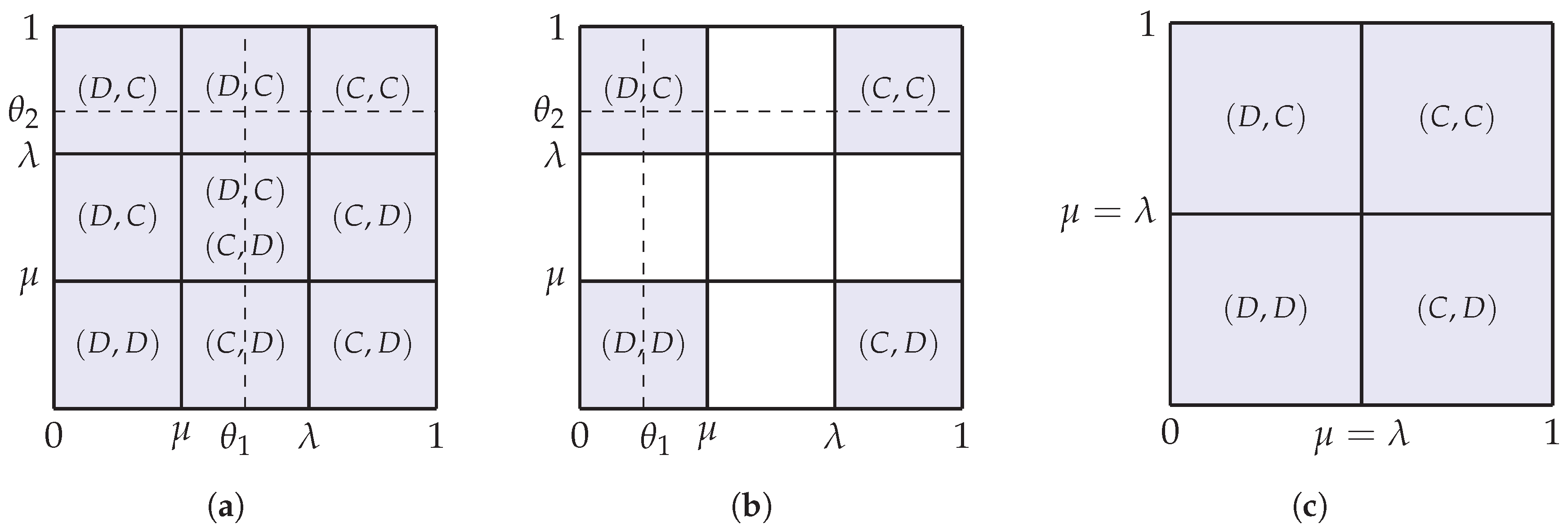
There are two different cases for extending this description of the NE for all possible continuous types, i.e., pairs $({\theta }_1,{\theta }_2)\in {[0,1]}^2$, depending on the relative values of the two parameters: (i) $\mu \le \lambda$; or (ii) $\mu \ge \lambda$. These two cases are broadly similar and we only consider Case (i). In this case, a simple analysis similar to the case of the boundary segments leads to Figure 1a which shows a NE for every pair $({\theta }_1,{\theta }_2)\in {[0,1]}^2$ [41]. This figure shows the set of NE for every pair of types in the interior of each of the nine sub-squares in ${[0,1]}^2$. Only the middle region contains two NEs at every point. On a boundary point of each sub-square, the set of NE is the union of the set of NE in the interiors of the sub-squares adjacent to the boundary point. For example, the local game $G_{(\mu ,\mu )}$ has three NEs: $(D,D),(C,D),(D,C)$.

Assume, first, that $\mu <\lambda$. When the whole unit square is the type profile space, shown as shaded in Figure 1a, it is easily seen that there exists no compatible pure ex post NE since Agent 1 cannot have $s_1\left({\theta }_1\right)=C$ or $s_1\left({\theta }_1\right)=D$ for $\mu <{\theta }_1<\lambda$, as depicted in Figure 1a, and similarly for Agent 2. If, however, ${\mathsf{\Theta }}_1,{\mathsf{\Theta }}_2\subseteq [0,\mu ]\cup [\lambda ,1]$, e.g., ${\mathsf{\Theta }}_1={\mathsf{\Theta }}_2=[0,\mu ]\cup [\lambda ,1]$ as shaded in Figure 1b, then there exists a unique compatible pure ex post NE for the standard uniform double game with $s_i\left({\theta }_i\right)=D$ for ${\theta }_i\in [0,\mu ]$ and $s_i\left({\theta }_i\right)=C$ for ${\theta }_i\in [\lambda ,1]$.

Assume next that $\mu =\lambda$ with ${\mathsf{\Theta }}_1={\mathsf{\Theta }}_2=[0,1]$ as in Figure 1c. Then, there are four compatible ex post NE as we can have $s_1\left(\mu \right)=C$ or $s_1\left(\mu \right)=D$ and $s_2\left(\mu \right)=C$ or $s_2\left(\mu \right)=D$. Observe that in Figure 1a, there exists no pure ex post NE on the boundary of the type profile space ${[0,1]}^2$, whereas in Figure 1b,c there exists a compatible pure ex post NE on the boundary which extends to the whole type profile space. Because the utilities in multigames are linear, we can postulate that this latter property extends to any standard uniform multigame. In fact, the main results of this paper are to show that this property holds and develop an algorithm which takes a compatible pure ex post NE on the vertices of the type profile space of a standard uniform multigame and determines in linear time with respect to the number of types if the compatible pure ex post NE extends to the boundary and thus to the whole type profile space.

Numerical Examples of Computation of Ex Post NE

We examine two numerical instances of the running example which show how the multigame representation can facilitate the computation of ex post NE in the class of linear multidimensional Bayesian games.

Example 1.

In the running example, let utilities for agents $i=1,2$ in PD and SG be given according to

Table 2. Utilities for PD (left) and SG (right) in Example 1.

	C	D		C	D
C	(6, 6)	(1, 7)	C	(5, 5)	(5, 1)
D	(7, 1)	(2, 2)	D	(1, 5)	(1, 1)

. By Equation (2), we obtain $\mu =\lambda =1/5$. Assume ${\mathsf{\Theta }}_i=[0,1]$ for $i=1,2$. Thus, Figure 1c shows that $(s_1(·),s_2(·))$ is an ex post NE for the game where $s_i\left({\theta }_i\right)=D$ if ${\theta }_i\le 1/5$ and $s_i\left({\theta }_i\right)=C$ otherwise for $i=1,2$.

Example 2.

In the running example, let utilities for agents $i=1,2$ in PD and SG be given according to

Table 3. Utilities for PD (left) and SG (right) in Example 2.

	C	D		C	D
C	(16, 16)	(3, 20)	C	(15, 15)	(15, 3)
D	(20, 3)	(6, 6)	D	(3, 15)	(3, 3)

. Assume ${\mathsf{\Theta }}_i=\{t/10:t=0,\dots ,10\}$ for $i=1,2$. By Equation (2), we obtain $\mu =1/5$ and $\lambda =1/4$. Since ${\mathsf{\Theta }}_i\cap (\mu ,\lambda )=\varnothing$ for each $i=1,2$, similar to Figure 1b, we see that $(s_1(·),s_2(·))$ is an ex post NE for the game where $s_i\left({\theta }_i\right)=D$ if ${\theta }_i\le 1/5$ and $s_i\left({\theta }_i\right)=C$ otherwise for $i=1,2$.

5. Pure Ex Post NE Induced From Type Profile Space Boundary

The computation of a NE in classical game theory is a hard problem in relation to the number of agents and strategies, which is why in applications one uses small numbers of agents and strategies (see [42]). Likewise, in applications of standard uniform multigames, we always deal with small n and m, but here the number of types can be large. This means that computation of an ex post NE in standard uniform multigames is a hard problem with respect to the number of types even for small numbers of agents and basic games. We show in this section that, if a standard uniform multigame has a compatible pure ex post NE on the boundary of the type profile space, then the game has a compatible pure ex post NE. In the case of a finite number of discrete types, we then derive an algorithm, linear in the number of types, to decide if a standard uniform multigame has a compatible pure ex post NE if it has one on its extreme type profiles ${\mathsf{\Theta }}^e$.

5.1. Partition of Type Profile Spaces

The following result gives an equivalent characterisation for the existence of a compatible pure ex post NE for a standard uniform multigame, which sheds light on the structure of the agents’ type spaces, namely their split into different regions as in the examples of Figure 1b,c.

Proposition 5.

Let G be a standard uniform multigame. Then, G has a compatible pure ex post NE if and only if, for each agent i, there are subsets ${\mathsf{\Theta }}_{ij}$ for $1\le j\le m$ such that

(i) 

${\mathsf{\Theta }}_i={\bigcup }_{1\le j\le m}{\mathsf{\Theta }}_{ij}$ with ${\mathsf{\Theta }}_{ij}\cap {\mathsf{\Theta }}_{ik}=\varnothing$ for $s_{ij}\ne s_{ik}$ and ${\mathsf{\Theta }}_{ij}={\mathsf{\Theta }}_{ik}=\varnothing$ for $s_{ij}=s_{ik}$ for $j,k\in J$;

(ii) 

$p_j\in {\mathsf{\Theta }}_{ij}$ for $1\le j\le m$; and

(iii) 

for all $\theta \in \mathsf{\Theta }$, the local game $G_{({\theta }_1,\dots ,{\theta }_n)}$ has as a NE the action profile $(s_{1j_1},\dots ,s_{i{j}_i},\dots ,s_{n{j}_n})$, where $j_i$ is given by ${\theta }_i\in {\mathsf{\Theta }}_{i{j}_i}$ for $1\le i\le n$.

Proof. 

Suppose G has a compatible pure ex post NE $(s_1(·),\dots ,s_n(·))$. For each agent i, let ${\mathsf{\Theta }}_{ij}={\left(s_i\right)}^{-1}\left(s_{ij}\right)$, where ${\left(s_i\right)}^{-1}$ is the inverse map of $s_i$ and, recall, $s_{ij}$ is the agent i’s action in the action profile $(s_{1j},\dots ,s_{ij},\dots ,s_{nj})$ that is a NE for the game $G_j$. Then, Condition (i) holds, and $p_j\in {\mathsf{\Theta }}_{ij}$ by Definition 9. Moreover, by Definition 7, $(s_{1j_1},\dots ,s_{i{j}_i},\dots ,s_{n{j}_n})$, where $j_i$ is given by ${\theta }_i\in {\mathsf{\Theta }}_{i{j}_i}$, is a NE for $G_{({\theta }_1,\dots ,{\theta }_n)}$. Next, suppose Conditions (i), (ii) and (iii) hold. Let $s_i(·):{\pi }_i\left[\mathsf{\Theta }\right]\to A_i$ be given by $s_i\left({\theta }_i\right)=s_{ij}$ where j is such that ${\theta }_i\in {\mathsf{\Theta }}_{ij}$. Condition (ii) shows that $s_i\left(p_j\right)=s_{ij}$ for each $i\in I$ and $j\in J$. In addition, we have $(s_1\left({\theta }_1\right),\dots ,s_n\left({\theta }_n\right))=(s_{1j_1},\dots ,s_{n{j}_n})$ where ${\theta }_i\in {\mathsf{\Theta }}_{i{j}_i}$. Thus, by Condition (iii), $(s_1\left({\theta }_1\right),\dots ,s_n\left({\theta }_n\right))$ is a NE for $G_{({\theta }_1,\dots ,{\theta }_n)}$. □

Running example continued: In the case of the standard uniform multigame of Figure 1b, where there is a unique compatible pure ex post NE, we have: ${\mathsf{\Theta }}_{i1}=[0,\mu ]$ and ${\mathsf{\Theta }}_{i2}=[\lambda ,1]$ for both agents $i=1,2$. For the standard uniform multigame of Figure 1c, each partition of $[0,1]$ for the four compatible pure ex post NE consists of ${\mathsf{\Theta }}_{i1}=[0,\mu )$ and ${\mathsf{\Theta }}_{i2}=[\mu ,1]$ or ${\mathsf{\Theta }}_{i1}=[0,\mu ]$ and ${\mathsf{\Theta }}_{i2}=(\mu ,1]$ for $i=1,2$.

5.2. Partition of an Agent’s Type Space Given Other Agents’ Types

In this section, we show that we obtain a partition of an agent’s type space, similar to Proposition 5, if we have a compatible pure ex post NE on the set of extreme types of the agent given the types of all other agents. We start by proving a property which generalises the existence of $\mu$ (or $\lambda$) in the running example (see Figure 1). We first show it in the case of double games with a constructive proof, which provides the intuitive idea behind it.

Lemma 1.

Let G be a standard uniform two-agent double game with $A_1=\{s,t\}$ and $A_2=\{u,v\}$. Assume that the strategy profiles $(s,u)$ and $(s,v)$ are NEs for $G_{({\theta }_1,0)}$ and $G_{({\theta }_1,1)}$ for ${\theta }_1\in {\mathsf{\Theta }}_1$. Then, there exists ${\theta }_2^{\ast }\in {\mathsf{\Theta }}_2$, independent of ${\theta }_1\in {\mathsf{\Theta }}_1$, such that $(s,u)$ is NE for $G_{({\theta }_1,{\theta }_2)}$ if ${\theta }_2\le {\theta }_2^{\ast }$ and $(s,v)$, respectively, if ${\theta }_2>{\theta }_2^{\ast }$.

Proof. 

Assume that the utilities of the two basic games are as in

Table 4. Utilities for $G_1$ (left) and $G_2$ (right) in Lemma 1.

	u	v		u	v
s	$(b_1,b_2)$	$(d_1,d_2)$	s	$(g_1,g_2)$	$(h_1,h_2)$
t	$(e_1,e_2)$	$(f_1,f_2)$	t	$(k_1,k_2)$	$({\ell }_1,{\ell }_2)$

. Since $(s,u)$ and $(s,v)$ are NEs for the local games $G_{({\theta }_1,0)}$ and $G_{({\theta }_1,1)}$, respectively, we have $U_2(s,u,{\theta }_1,0)\ge U_2(s,v,{\theta }_1,0)$ and also $U_2(s,v,{\theta }_1,1)\ge U_2(s,u,{\theta }_1,1)$ which imply $b_2\ge d_2$ and $h_2\ge g_2$. Let $f\left({\theta }_2\right)=U_2(s,u,{\theta }_1,{\theta }_2)-U_2(s,v,{\theta }_1,{\theta }_2)$, i.e., $f\left({\theta }_2\right)={\theta }_2(g_2-h_2+d_2-b_2)+b_2-d_2$. If $g_2-h_2+d_2-b_2=0$ then $f\left({\theta }_2\right)\ge 0$ for each ${\theta }_2\in {\mathsf{\Theta }}_2$ and the strategy profile $(s,u)$ is NE for the local games $G_{({\theta }_1,{\theta }_2)}$ for all $0\le {\theta }_2\le 1$. In this case, put ${\theta }_2^{\ast }=1$. Next, suppose $g_2-h_2+d_2-b_2\ne 0$. Let

$${\theta }_2^{\ast }=\frac{b_2-d_2}{b_2-d_2+h_2-g_2}.$$

Since $b_2\ge d_2$ and $h_2\ge g_2$, we have $0\le {\theta }_2^{\ast }\le 1$ and $f({\theta }_2)\ge 0$ for ${\theta }_2\le {\theta }_2^{\ast }$ and $f\left({\theta }_2\right)\le 0$ for ${\theta }_2^{\ast }<{\theta }_2$ and the result follows. □

Running example continued: Considering the double game for PD in the three diagrams in Figure 1a–c, we see that, in all three cases, for any value of ${\theta }_1$ with $0\le {\theta }_1\le \mu$, we have the two NE’s $(D,D)$ and $(D,C)$ for ${\theta }_2=0$ and ${\theta }_2=1$, respectively. In Figure 1a–c, we see that ${\theta }_2^{\ast }=\mu$ is independent of ${\theta }_1\in [0,\mu ]$ as stipulated by Lemma 1. A similar result is observed for ${\theta }_1\in [\lambda ,1]$ with $(C,D)$ and $(C,C)$ as NEs for ${\theta }_2=0$ and ${\theta }_2=1$, respectively, with ${\theta }_2^{\ast }=\lambda$ independent of ${\theta }_1\in [\lambda ,1]$.

We next obtain the extension of Lemma 1 for the general case of a multigame, which uses a proof by contradiction.

Lemma 2.

Let a standard uniform multigame G have a compatible pure ex post NE $(s_i(·),s_{-i}(·))$ on ${\mathsf{\Theta }}_i^e\times \left\{{\theta }_{-i}\right\}$ for a given agent $i\in I$ and ${\theta }_{-i}\in {\mathsf{\Theta }}_{-i}$. Then, there exists ${\mathsf{\Theta }}_{ij}\left({\theta }_{-i}\right)\subseteq {\mathsf{\Theta }}_i$, for each $j\in J$, such that

1. 

${\mathsf{\Theta }}_i={\bigcup }_{j\in J}{\mathsf{\Theta }}_{ij}\left({\theta }_{-i}\right)$ where ${\mathsf{\Theta }}_{ij}\left({\theta }_{-i}\right)\cap {\mathsf{\Theta }}_{ik}\left({\theta }_{-i}\right)=\varnothing$ for $j,k\in J$ with $j\ne k$; and

2. 

given ${\theta }_i\in {\mathsf{\Theta }}_i$, the local game $G_{({\theta }_i,{\theta }_{-i})}$ has a NE for a strategy profile $\left(s_i(p_j),s_{-i}({\theta }_{-i})\right)$, where $j\in J$ is the game for which ${\theta }_i\in {\mathsf{\Theta }}_{ij}({\theta }_{-i})$.

Proof. 

For a pure ex post NE $(s_i\left(p_j\right),s_{-i}\left({\theta }_{-i}\right))\in S_i\times S_{-i}$, of G on ${\mathsf{\Theta }}_i^e\times \{{\theta }_{-i}\}$ for agent i and for $j\in J$, let $P_j:{\mathsf{\Theta }}_i\to \mathbb{R}$ be the plane

$$P_j\left({\theta }_i\right)=U_i(s_i\left(p_j\right),s_{-i}\left({\theta }_{-i}\right),{\theta }_i,{\theta }_{-i}),$$

for $j\in J$. For each $k,j\in J$, put

$$T_{jk}:=\left\{{\theta }_i\in {\mathsf{\Theta }}_i|P_j\left({\theta }_i\right)-P_k\left({\theta }_i\right)\ge 0\right\}.$$

Let ${\mathsf{\Theta }}_{i1}\left({\theta }_{-i}\right)={\bigcap }_{k=1}^m{T}_{1k}$ and, for $j>1$, ${\mathsf{\Theta }}_{ij}\left({\theta }_{-i}\right)=\{{\theta }_i\in {\mathsf{\Theta }}_i\backslash {\mathsf{\Theta }}_{i(j-1)}\left({\theta }_{-i}\right)\mid {\theta }_i\in {\bigcap }_{k=1}^m{T}_{jk}\}.$ We claim that ${\mathsf{\Theta }}_i={\bigcup }_{j\in J}{\mathsf{\Theta }}_{ij}\left({\theta }_{-i}\right)$. Suppose, for a contradiction, that there exists ${\theta }_i\in {\mathsf{\Theta }}_i\backslash {\bigcup }_{j\in J}{\mathsf{\Theta }}_{ij}\left({\theta }_{-i}\right)$. Then, there exists $j_1\in J$ such that ${\theta }_i\notin T_{1j_1}$ as ${\theta }_i\notin {\mathsf{\Theta }}_{i1}\left({\theta }_{-i}\right)$. Since ${\theta }_i\notin {\mathsf{\Theta }}_{i{j}_1}\left({\theta }_{-i}\right)$, there exists $j_2\in J$ such that ${\theta }_i\notin T_{j_1{j}_2}$. Inductively, for each integer $r>2$, there exists $j_r\in J$ such that ${\theta }_i\notin T_{j_{r-1}{j}_r}$. Put $j_0:=1$. Since J is finite, there exist $r,k\ge 0$ with $k<r$ and $j_r=j_k$. Thus,

$$\begin{array}{c}\hfill \left\{\begin{array}{ccccc}{P}_{j_{k+1}}\left({\theta }_i\right)& -& P_{j_k}\left({\theta }_i\right)& >& 0\\ P_{j_{k+2}}\left({\theta }_i\right)& -& P_{j_{k+1}}\left({\theta }_i\right)& >& 0\\ ⋮& ⋮& ⋮& ⋮& ⋮\\ P_{j_k}\left({\theta }_i\right)& -& P_{j_{r-1}}\left({\theta }_i\right)& >& 0.\end{array}\right.\end{array}$$

(3)

Adding Inequalities (3) yields: $P_{j_k}\left({\theta }_i\right)-P_{j_k}\left({\theta }_i\right)>0$, which is a contradiction. Therefore, ${\mathsf{\Theta }}_i={\bigcup }_{j\in J}{\mathsf{\Theta }}_{ij}\left({\theta }_{-i}\right)$, and, by construction, ${\mathsf{\Theta }}_{ij}\left({\theta }_{-i}\right)\cap {\mathsf{\Theta }}_{ik}\left({\theta }_{-i}\right)=\varnothing$ for each $j\ne k$. Assume that ${\theta }_i\in {\mathsf{\Theta }}_{ij}\left({\theta }_{-i}\right)$. Thus, we have

$$\begin{array}{c}\hfill U_i(s_i\left(p_j\right),s_{-i}\left({\theta }_{-i}\right),{\theta }_i,{\theta }_{-i})\ge U_i(s_i\left(p_k\right),s_{-i}\left({\theta }_{-i}\right),{\theta }_i,{\theta }_{-i})\end{array}$$

for each $k\in J$. By the assumption, we have: $A_i=\{s_i\left(p_j\right):j\in J\}$. Hence, for each $a_i\in A_i$, we have

$$U_i(s_i\left(p_j\right),s_{-i}\left({\theta }_{-i}\right),{\theta }_i,{\theta }_{-i})\ge U_i(a_i,s_{-i}\left({\theta }_{-i}\right),{\theta }_i,{\theta }_{-i}),$$

i.e., the strategy profile $\left(s_i\left(p_j\right),s_{-i}\left({\theta }_{-i}\right)\right)$ is a NE for $G_{({\theta }_i,{\theta }_{-i})}$ where ${\theta }_i\in {\mathsf{\Theta }}_{ij}\left({\theta }_{-i}\right)$ and $j\in J$. □

Note that the set ${\mathsf{\Theta }}_{ij}\left({\theta }_{-i}\right)$ in the statement of Lemma 2 can be empty for some $j>1$. It also follows from the construction of ${\mathsf{\Theta }}_{ij}\left({\theta }_{-i}\right)$ in the proof that if ${\mathsf{\Theta }}_{ij}\left({\theta }_{-i}\right)=\varnothing$ for some $j>1$ then ${\mathsf{\Theta }}_{ik}\left({\theta }_{-i}\right)=\varnothing$ for $j\le k\le m$. We can now define the notion of a partition of an agent’s type set.

Definition 10.

We call a family of subsets ${\mathsf{\Theta }}_{ij}\left({\theta }_{-i}\right)\subseteq {\mathsf{\Theta }}_i$, for agent i with $j\in J$, satisfying Conditions 1 and 2 of Lemma 2 a partition of ${\mathsf{\Theta }}_i$ with respect to ${\theta }_{-i}$.

Running example continued: The partitions of ${\mathsf{\Theta }}_1$ with respect to the two possible values ${\theta }_{-1}={\theta }_2=0$ and 1 for the three double games in Figure 1a–c are. respectively as follows: (a) ${\mathsf{\Theta }}_{11}\left(0\right)=[0,\mu ]$, ${\mathsf{\Theta }}_{12}\left(0\right)=(\mu ,1]$, ${\mathsf{\Theta }}_{11}\left(1\right)=[0,\lambda ]$, ${\mathsf{\Theta }}_{12}\left(1\right)=(\lambda ,1]$; (b) ${\mathsf{\Theta }}_{11}\left(0\right)=[0,\mu ]$, ${\mathsf{\Theta }}_{12}\left(0\right)=[\lambda ,1]$, ${\mathsf{\Theta }}_{11}\left(1\right)=[0,\mu ]$, ${\mathsf{\Theta }}_{12}\left(1\right)=[\lambda ,1]$; and (c) ${\mathsf{\Theta }}_{11}\left(0\right)=[0,\mu ]$, ${\mathsf{\Theta }}_{12}\left(0\right)=(\mu ,1]$, ${\mathsf{\Theta }}_{11}\left(1\right)=[0,\mu ]$, ${\mathsf{\Theta }}_{12}\left(1\right)=(\mu ,1]$. Note that in Case (a), in which there is no pure ex post NE, the partition is different for ${\theta }_{-1}={\theta }_2=0$ and 1, whereas, in Cases (b) and (c), in which there exists at least one ex post NE, the two partitions for ${\theta }_{-1}={\theta }_2=0$ and 1 are the same. We show later in Theorems 2 and 3 that these properties are instances of a more general result. We present two other examples first.

Example 3.

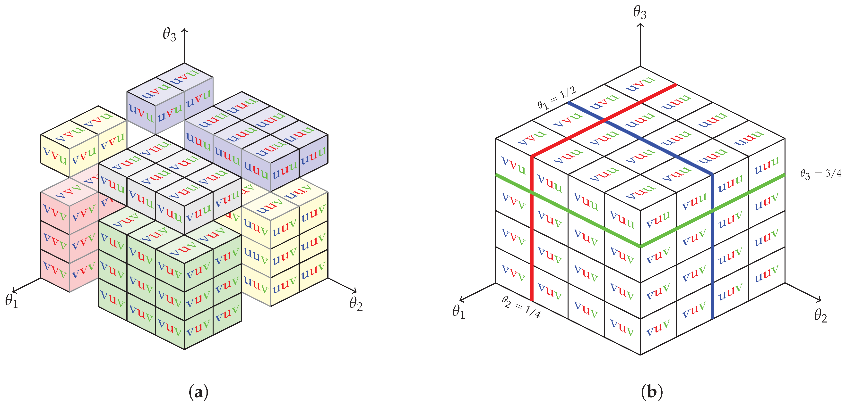
Suppose G is a standard uniform three-agent double game with basic games $G_1$ and $G_2$ where $A_i=\{u_i,v_i\}$ for $1\le i\le 3$ and $\mathsf{\Theta }={[0,1]}^3$ and assume the utilities of $G_1$ and $G_2$ are as in

Table 5. The utility matrix of Example 3 for the basic game $G_1$ for $a\in A_3$.

a = u3			a = v3
	u2	v2		u2	v2
$u_1$	$(1,10,3)$	$(6,9,9)$	$u_1$	$(12,3,0)$	$(3,1,6)$
$v_1$	$(0,11,11)$	$(4,7,10)$	$v_1$	$(9,13,8)$	$(-1,12,4)$

and

Table 6. The utility matrix of Example 3 for the basic game $G_2$ for $a\in A_3$.

a = u3			a = v3
	u2	v2		u2	v2
$u_1$	$(1,3,1)$	$(8,6,4)$	$u_1$	$(5,2,2)$	$(7,8,5)$
$v_1$	$(2,8,12)$	$(10,20,18)$	$v_1$	$(8,2,13)$	$(11,5,20)$

, respectively. Hence, $(u_1,u_2,u_3)$ and $(v_1,v_2,v_3)$ are, respectively, NEs for $G_1$ and $G_2$. Figure 2a shows the partition of $\mathsf{\Theta }={[0,1]}^3$ into $2^3$ regions of constant local NE, as described in Lemma 2, by the three planes ${\theta }_1=1/2$ (blue), ${\theta }_2=1/4$ (red) and ${\theta }_3=3/4$ (green) depicted in Figure 2. For convenience, we drop the brackets and commas in a strategy profile, e.g., the strategy profile $(u_1,v_2,u_3)$ is abbreviated as $uvu$. Thus, the partition of the type profile space ${[0,1]}^3$ represents a three dimensional extension of Figure 1c of the type space ${[0,1]}^2$ for the double game for PD with $\mu =\lambda$. For example, if $i=3$, then ${\theta }_{-3}=\{{\theta }_1,{\theta }_2\}$ and if $1/4\le {\theta }_1\le 1$ and $1/2\le {\theta }_2\le 1$, then we have ${\mathsf{\Theta }}_{31}\left({\theta }_{-3}\right)=[0,3/4]$ and ${\mathsf{\Theta }}_{32}\left({\theta }_{-3}\right)=(3/4,1]$ or ${\mathsf{\Theta }}_{31}\left({\theta }_{-3}\right)=[0,3/4)$ and ${\mathsf{\Theta }}_{32}\left({\theta }_{-3}\right)=[3/4,1]$.

Example 4.

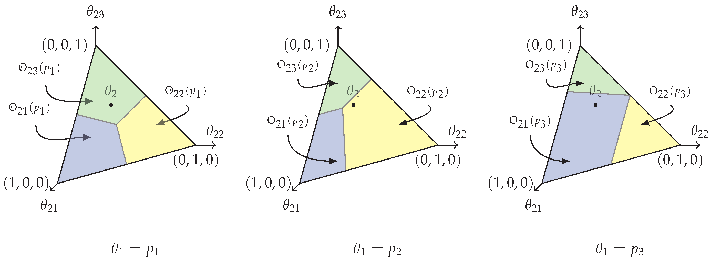
Suppose G is a standard uniform two-agent multigame with three basic games and $A_i=\{u_i,v_i,w_i\}$ for each $i\in I$. The utilities of $G_1$, $G_2$ and $G_3$ have been depicted in

Table 7. Utilities for basic games $G_1$, $G_2$ and $G_3$ of Example 4.

	${\mathit{u}}_2$	${\mathit{v}}_2$	${\mathit{w}}_2$		${\mathit{u}}_2$	${\mathit{v}}_2$	${\mathit{w}}_2$		${\mathit{u}}_2$	${\mathit{v}}_2$	${\mathit{w}}_2$
$u_1$	$(3,3)$	$(3,2)$	$(3,2)$	$u_1$	$(2,2)$	$(2,3)$	$(2,2)$	$u_1$	$(2,2)$	$(2,2)$	$(1,3)$
$v_1$	$(2,3)$	$(2,2.5)$	$(2,2)$	$v_1$	$(3,2)$	$(3,3)$	$(3,1)$	$v_1$	$(2,2)$	$(2,2)$	$(2,3)$
$w_1$	$(2,3)$	$(2,2)$	$(2,1)$	$w_1$	$(2,2)$	$(2,3)$	$(2,1)$	$w_1$	$(3,2)$	$(3,1)$	$(3,3)$

. The strategy profiles $(u_1,u_2)$, $(v_1,v_2)$ and $(w_1,w_2)$ are, respectively, NEs for the basic games $G_1$, $G_2$ and $G_3$.

Table 8. NE of $G_{({\theta }_1,{\theta }_2)}$ for all $({\theta }_1,{\theta }_2)\in {\mathsf{\Theta }}^e$.

	${\mathit{p}}_1$	${\mathit{p}}_2$	${\mathit{p}}_3$
$p_1$	$(u_1,u_2)$	$(u_1,v_2)$	$(u_1,w_2)$
$p_2$	$(v_1,u_2)$	$(v_1,v_2)$	$(v_1,w_2)$
$p_3$	$(w_1,u_2)$	$(w_1,v_2)$	$(w_1,w_2)$

gives the NE for all local games and shows that $(s_1(·),s_2(·))$ is a compatible pure ex post NE on ${\mathsf{\Theta }}^e$ where $s_i\left((1,0,0)\right)=u_i,s_i\left((0,1,0)\right)=v_i$ and $s_i\left((0,0,1)\right)=w_i$. The partition of ${\mathsf{\Theta }}_i$ for each $i=1,2$, as given by Lemma 2, is illustrated in Figure 3. Let ${\theta }_2=(1/4,1/4,1/2)$. We have: ${\theta }_2\in {\mathsf{\Theta }}_{23}\left(p_1\right)$ but ${\theta }_2\notin {\mathsf{\Theta }}_{23}\left(p_2\right)$ and ${\theta }_2\notin {\mathsf{\Theta }}_{23}\left(p_3\right)$. Therefore, ${\mathsf{\Theta }}_{23}\left({\theta }_1\right)$ is not independent of ${\theta }_1\in {\mathsf{\Theta }}_1^e$. In this case, the compatible pure ex post NE cannot be extended to ${\mathsf{\Theta }}^b$ since, as shown in Figure 3, none of the three actions $u_2,v_2,w_2$ for $s_2\left({\theta }_2\right)$, with the above value of ${\theta }_2$, can provide the three local NE at $(p_j,{\theta }_2)$ for $j=1,2,3$.

Main Results and Algorithm

We observe that, in the examples of the double game for PD of Figure 1b,c, as well as in Example 3, we have a compatible pure ex post NE on the extreme type profiles, i.e., on ${\mathsf{\Theta }}^e$, which extends to the boundary ${\mathsf{\Theta }}^b$. In all these cases, for each $i\in I$, the partitions ${({\mathsf{\Theta }}_{ij}({\theta }_{-i}))}_{j\in J}$ of ${\mathsf{\Theta }}_i$ are independent of ${\theta }_{-i}\in {\mathsf{\Theta }}_{-i}^e$. In contrast, in the example of the double game for PD of Figure 1a and in Example 4, we have a compatible pure ex post NE on ${\mathsf{\Theta }}^e$ which does not extend to ${\mathsf{\Theta }}^b$. In these two cases, the partitions ${({\mathsf{\Theta }}_{ij}({\theta }_{-i}))}_{j\in J}$ of ${\mathsf{\Theta }}_i$ are not independent of ${\theta }_{-i}\in {\mathsf{\Theta }}_{-i}^e$. In fact, we have the following general result.

Theorem 2.

Let G be a standard uniform multigame with a compatible pure ex post NE $(s_1(·),\dots ,s_n(·))$ on ${\mathsf{\Theta }}^e$. Then, the following two conditions are equivalent.

(i) 

$(s_1(·),\dots ,s_n(·))$ is a compatible pure ex post NE for G on ${\mathsf{\Theta }}^b$.

(ii) 

For each agent $i\in I$ and ${\theta }_{-i}\in {\mathsf{\Theta }}_{-i}$ there exists a partition ${\left\{{\mathsf{\Theta }}_{ij}\left({\theta }_{-i}\right)\right\}}_{j\in J}$ of ${\mathsf{\Theta }}_i$ with ${\mathsf{\Theta }}_i={\bigcup }_{j\in J}{\mathsf{\Theta }}_{ij}\left({\theta }_{-i}\right)$ such that the set ${\mathsf{\Theta }}_{ij}\left({\theta }_{-i}\right)$ is independent of ${\theta }_{-i}\in {\mathsf{\Theta }}_{-i}^e$ for each $j\in J$.

Proof. 

Suppose Condition (ii) holds. Then, ${\mathsf{\Theta }}_i={\bigcup }_{j\in J}{\mathsf{\Theta }}_{ij}$ and from the definition of a partition (Definition 10), it follows that the strategy profile $\left(s_i\left(p_j\right),s_{-i}\left({\theta }_{-i}\right)\right)$ is a NE for the local game $G_{({\theta }_i,{\theta }_{-i})}$ where ${\theta }_i\in {\mathsf{\Theta }}_{ij}$ and ${\theta }_{-i}\in {\mathsf{\Theta }}_{-i}^e$. Hence, $\left(s_i\left(p_j\right),s_{-i}\left({\theta }_{-i}\right)\right)$ is a NE for G on ${\mathsf{\Theta }}^b$.

For the converse, suppose $(s_1(·),\dots ,s_n(·))$ is a compatible pure ex post NE for G on ${\mathsf{\Theta }}^b$. Then, for each $i\in I$, we have $A_i=\{s_i\left(p_j\right):j\in J\}$ and for each ${\theta }_i\in {\mathsf{\Theta }}_i$, there exists $j\in J$ such that the strategy profile $(s_i\left(p_j\right),s_{-i}\left({\theta }_{-i}\right))$ is a NE for the local game $G_{({\theta }_i,{\theta }_{-i})}$ for all ${\theta }_{-i}\in {\mathsf{\Theta }}_{-i}^e$. Construct ${\mathsf{\Theta }}_{ij}$ inductively as follows. Let ${\mathsf{\Theta }}_{i1}\subseteq {\mathsf{\Theta }}_i$ where $(s_i\left(p_1\right),s_{-i}\left({\theta }_{-i}\right))$ is a NE for the local game $G_{({\theta }_i,{\theta }_{-i})}$ for ${\theta }_i\in {\mathsf{\Theta }}_{i1}$ and ${\theta }_{-i}\in {\mathsf{\Theta }}_{-i}^e$. Next, for each $1\le j\le m-1$, iteratively construct ${\mathsf{\Theta }}_{i(j+1)}\subseteq {\mathsf{\Theta }}_i\backslash {\bigcup }_{1\le k\le j}{\mathsf{\Theta }}_{ik}$ such that for each ${\theta }_i\in {\mathsf{\Theta }}_{i(j+1)}$, the strategy profile $(s_i\left(p_{j+1}\right),s_{-i}\left({\theta }_{-i}\right))$ is a NE for the local game $G_{({\theta }_i,{\theta }_{-i})}$ for all ${\theta }_{-i}\in {\mathsf{\Theta }}_{-i}^e$. Then, ${\mathsf{\Theta }}_{ij}$ are disjoint for $j\in J$ and we have ${\mathsf{\Theta }}_i={\bigcup }_{j\in J}{\mathsf{\Theta }}_{ij}$ as required. □

We can now deduce one of our main results for a standard uniform multigame.

Theorem 3.

A standard uniform multi-game has a compatible pure ex post NE if and only if it has a compatible pure ex post NE on the boundary ${\mathsf{\Theta }}^b$ of the type profile space Θ.

Proof. 

The “only if” part follows immediately from the definition of Definition 9. Suppose the standard uniform multigame G has a compatible pure ex post NE on ${\mathsf{\Theta }}^b$. Then, for each $i\in I$, there exists $s_i:{\mathsf{\Theta }}_i\to A_i$ and $s_{-i}:{\mathsf{\Theta }}_{-i}^e\to A_{-i}$ such that $(s_i\left({\theta }_i\right),s_{-i}\left({\theta }_{-i}\right))$ is a NE for $G_{({\theta }_i,{\theta }_{-i})}$ for each $({\theta }_i,{\theta }_{-i})\in {\mathsf{\Theta }}_i\times {\mathsf{\Theta }}_{-i}^e$. Since $A_i=\{s_i\left(p_j\right):j\in J\}$, there exists $j_i\in J$ for each $i\in$ such that $s_i\left({\theta }_i\right)=s_i\left(p_{j_i}\right)$. Thus, there exists $j_r\in J$, for each $r\in I$, such that $(s_1\left({\theta }_1\right),\dots ,s_n\left({\theta }_n\right))=(s_1\left(p_{j_1}\right),\dots ,s_n\left(p_{j_n}\right))$, for each $({\theta }_1,\dots ,{\theta }_n)\in \mathsf{\Theta }$. We claim $(s_1\left({\theta }_1\right),\dots ,s_n\left({\theta }_n\right))$ is a NE for $G_{({\theta }_1,\dots ,{\theta }_n)}$ for each $({\theta }_1,\dots ,{\theta }_n)\in \mathsf{\Theta }$. We have, for each $i\in I$,

$$\begin{array}{c}\hfill U_i(s_i\left({\theta }_i\right),s_{-i}\left({\theta }_{-i}\right),{\theta }_i,{\theta }_{-i})=U_i(s_i\left(p_{j_i}\right),s_{-i}\left({\theta }_{-i}\right),{\theta }_i,{\theta }_{-i})=\sum _{j\in J}{\theta }_{ij}{U}_{ij}(s_i\left(p_{j_i}\right),s_{-i}\left({\theta }_{-i}\right)).\end{array}$$

Let $i\in I$ and $a_i\in S_i$ be given. Since $(s_i\left({\theta }_i\right),s_{-i}\left({\theta }_{-i}\right))$ is a NE for $G_{(p_{j_1},\dots ,p_{j_{i-1}},{\theta }_i,p_{j_{i+1}},\dots ,p_{j_n})}$, it follows that ${\sum }_{j\in J}{\theta }_{ij}{U}_{ij}(s_i(p_{j_i}),s_{-i}({\theta }_{-i}))\ge {\sum }_{j\in J}{\theta }_{ij}{U}_{ij}(a_i,s_{-i}({\theta }_{-i})),$ for each $({\theta }_i,{\theta }_{-i})\in {\mathsf{\Theta }}_i\times {\mathsf{\Theta }}_{-i}$. Hence, $U_i(s_i\left({\theta }_i\right),s_{-i}\left({\theta }_{-i}\right),{\theta }_i,{\theta }_{-i})\ge U_i(a_i,s_{-i}\left({\theta }_{-i}\right),{\theta }_i,{\theta }_{-i})$ for each $({\theta }_i,{\theta }_{-i})\in {\mathsf{\Theta }}_i\times {\mathsf{\Theta }}_{-i}$, as required. □

By Theorem 3, Example 3 has a compatible pure ex post NE and Example 4 has no compatible pure ex post NE. From Theorems 3 and 2, we obtain:

Corollary 1.

Let standard uniform multigame G have a compatible pure ex post NE on ${\mathsf{\Theta }}^e$. Then, G has a pure ex post NE if for each $i\in I$ and $j\in J$ the set ${\mathsf{\Theta }}_{ij}\left({\theta }_{-i}\right)$ in the partition of ${\mathsf{\Theta }}_i$ is independent of ${\theta }_{-i}\in {\mathsf{\Theta }}_{-i}^e$.

Assume now that the type space ${\mathsf{\Theta }}_i$ is finite for each agent $i\in I$. Based on Corollary 1, we can derive an algorithm to check whether a standard uniform multigame with a compatible pure ex post NE on ${\mathsf{\Theta }}^e$, has a pure ex post NE on ${\mathsf{\Theta }}^b$, in which cases, by Theorem 3, it will have a compatible pure ex post NE. If the strategy profile ${\left\{(s_i\left(p_1\right),\dots ,s_i\left(p_m\right))\right\}}_{i\in I}$ is a compatible pure ex post NE of G on ${\mathsf{\Theta }}^e$, we define:

$$\mathsf{T}(i;(s_i\left(p_1\right),\dots ,s_i\left(p_m\right));{\theta }_{-i})=\prod _{j\in J}{\mathsf{\Theta }}_{ij}\left({\theta }_{-i}\right),$$

where ${\mathsf{\Theta }}_{ij}\left({\theta }_{-i}\right)$ for $j\in J$ is given in Lemma 2. Consider now Algorithm 1. The number of calls to $\mathsf{T}(i;(s_i\left(p_1\right),\dots ,s_i\left(p_m\right));{\theta }_{-i})$ is $n{m}^{n-1}$. Moreover, the runtime of $\mathsf{T}$ for ${\theta }_{-i}\in {\mathsf{\Theta }}_{-i}^e$ is $O(|{\mathsf{\Theta }}_i|)$. Thus, the computational complexity of Algorithm 1 is $O(kn{m}^{n-1})$ where $k={max}_{i\in I}|{\mathsf{\Theta }}_i|$. Therefore, for small n and m as we have in applications, Algorithm 1 is linear with respect to the size of the type profile space.

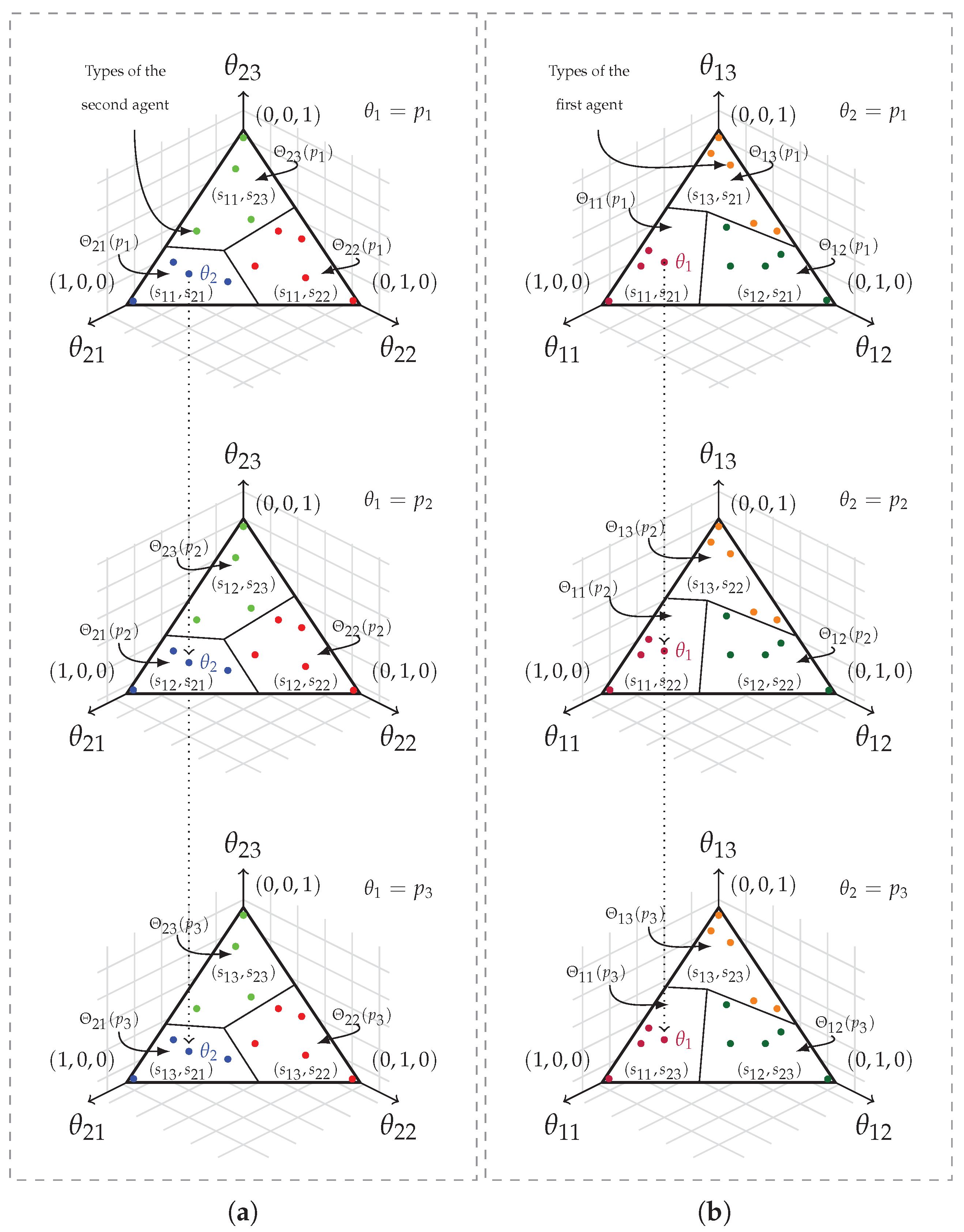
As an example, Figure 4 illustrates a two-agent standard uniform multigame G with 3 basic games and ${\mathsf{\Theta }}_1,{\mathsf{\Theta }}_2\subseteq {\Delta }^2$ where the types of each agent are shown by small discs. In the figure, we see that, for each $i\in I$ and $j\in J$, the set ${\mathsf{\Theta }}_{ij}\left({\theta }_{-i}\right)$ is independent of ${\theta }_{-i}$. Theorem 2 implies that G has a pure ex post NE on ${\mathsf{\Theta }}^b$. Hence, G has a pure ex post NE by Theorem 3 and the ex post NE can be efficiently computed by Algorithm 1.

Algorithm 1: The test for the existence of a pure ex post NE

6. Pure Ex Post NEs in Multimarkets

In this section, we present two different types of standard uniform games in multimarkets.

6.1. Adoption of Technology

Consider n companies, competing in a multi-market, which have to adopt a long-term strategy as to whether they should implement a new technology in their production (e.g., energy companies choosing between fossil-based or renewable sources of energy). Due to the high cost of shifting to the new technology, they need to use the same strategy in all the available markets. We thus have a standard uniform game in which the agents have two possible strategies.

We model one such scenario with two firms $(i=1,2)$, each with the choice either to adopt (a) or to reject (r) the new technology. Suppose the two firms compete in two markets $j=1,2$, where they have different costs for the adoption of the new technology as well as different returns from the adoption. The strategy space for both firms is given by $\{a,r\}$. Assume

Table 9. Utilities for markets $G_1$ and $G_2$.

	a	r		a	r
a	$(b_1,b_2)$	$(d_1,d_2)$	a	$(g_1,g_2)$	$(h_1,h_2)$
r	$(e_1,e_2)$	$(f_1,f_2)$	r	$(k_1,k_2)$	$({\ell }_1,{\ell }_2)$

shows utilities for firms in market $G_1$ and market $G_2$, respectively. Let $b_1>e_1,{\ell }_1>h_1$ and $b_2>d_2,{\ell }_2>k_2$. Then, the strategy profiles $(a,a)$ and $(r,r)$ are NEs for $G_1$ and $G_2$, respectively. Assume $k_1>g_1$, $d_1>f_1$, $h_2>g_2$, and $e_2>f_2$. These inequalities guarantee that the double game has a compatible pure ex post NE on ${\mathsf{\Theta }}^e$. Furthermore, suppose $(k_1-g_1)/(b_1-e_1)=({\ell }_1-h_1)/(d_1-f_1)$ and $(h_2-g_2)/(b_2-d_2)=({\ell }_2-k_2)/(e_2-f_2)$. Then, the double game has a pure ex post NE on the boundary. Theorem 3 implies that the double game has a pure ex post NE If $b_1-e_1+k_1-g_1=0$, then let ${\theta }_1^{\ast }=1$; otherwise, let ${\theta }_1^{\ast }=(b_1-e_1)/(b_1-e_1+k_1-g_1)$. Similarly, if $b_2-d_2+h_2-g_2=0$, then let ${\theta }_2^{\ast }=1$; otherwise, let ${\theta }_2^{\ast }=(b_2-d_2)/(b_2-d_2+h_2-g_2)$. Hence, $(s_1(·),s_2(·))$ is an ex post NE where $s_i(·):{\mathsf{\Theta }}_i\to \{a,r\}$ is given by $s_i\left({\theta }_i\right)=a$ if ${\theta }_i\le {\theta }_i^{\ast }$ and $s_i\left({\theta }_i\right)=r$ otherwise.

6.2. Multimarket Production

Consider n multinational companies which compete in multimarkets consisting of, e.g., m different markets each with its own rate of return. Assume that, for each $j\in J=\{1,\dots m\}$, a given product $s_{ij}$ is NE inducing for company $i\in I$, but, due to the design and manufacturing costs, each company has to produce the same product in all the m markets. In this way, we have a standard uniform multigame with $A_i=\{s_{ij}:j\in J\}$ for each $i\in I$ where ${\theta }_{ij}$ is the investment fraction of company i in market j.

We present a numerical example which models the competition of two companies (e.g., two multinational smart-phone producers) which can invest in three markets (e.g., the national economies of the US, EU and China). Assume the three markets are represented by three basic games $G_1$, $G_2$ and $G_3$ whose utilities are shown in

Table 10. Utilities for basic games $G_1$, $G_2$ and $G_3$.

	${\mathit{s}}_{21}$	${\mathit{s}}_{22}$	${\mathit{s}}_{23}$		${\mathit{s}}_{21}$	${\mathit{s}}_{22}$	${\mathit{s}}_{23}$		${\mathit{s}}_{21}$	${\mathit{s}}_{22}$	${\mathit{s}}_{23}$
$s_{11}$	$(3,7)$	$(11,4)$	$(4,3)$	$s_{11}$	$(4,1)$	$(5,4)$	$(9,2)$	$s_{11}$	$(2,2)$	$(3,6)$	$(7,10)$
$s_{12}$	$(2,8)$	$(10,5)$	$(3,4)$	$s_{12}$	$(5,5)$	$(6,8)$	$(10,6)$	$s_{12}$	$(4,4)$	$(6,8)$	$(8,12)$
$s_{13}$	$(1,5)$	$(9,2)$	$(2,1)$	$s_{13}$	$(3,0)$	$(4,3)$	$(8,1)$	$s_{13}$	$(3,6)$	$(5,10)$	$(9,14)$

with ${\mathsf{\Theta }}_i={\Delta }^2$ and $A_i=\{s_{ij}:1\le j\le 3\}$ for each company $i=1,2$. Recall that, for each $1\le j\le 3$, the strategy profile $(s_{1j},s_{2j})$ is a NE for the basic game $G_j$. For each company $i=1,2$, let $s_i(·):{\mathsf{\Theta }}_i^e\to A_i$ be given by $s_i\left(p_j\right)=s_{ij}$ for each $1\le j\le 3$. For each vector $x\in {\mathbb{R}}^m$, we write $x=(x_1,\cdots ,x_m)\ge 0$ if $x_r\ge 0$ for each $0\le r\le m$, and we denote the transpose of x by $x^t$.

Using, step by step, the method of proof in Lemma 2 and Theorem 2, we show that the multigame has an ex post NE. We start by putting $i=1$ and ${\theta }_{-i}=p_1$. Let $P_j:{\Delta }^2\to \mathbb{R}$ be the plane $P_j\left({\theta }_1\right)=U_1(s_1\left(p_j\right),s_2\left(p_1\right),{\theta }_1,p_1),$ for $1\le j\le 3$. Thus, $P_1\left({\theta }_1\right)={\theta }_{11}+2{\theta }_{12}+2$, $P_2\left({\theta }_1\right)=-2{\theta }_{11}+{\theta }_{12}+4$ and $P_3\left({\theta }_1\right)=-2{\theta }_{11}+3$ where ${\theta }_1=({\theta }_{11},{\theta }_{12},1-{\theta }_{11}-{\theta }_{12})$. Put $T_{jk}:=\left\{{\theta }_1\in {\Delta }^2|P_j\left({\theta }_1\right)-P_k\left({\theta }_1\right)\ge 0\right\}$, for each $1\le k,j\le 3$ and let ${\mathsf{\Theta }}_{11}\left(p_1\right)={\bigcap }_{k=1}^3{T}_{1k}$ and ${\mathsf{\Theta }}_{1j}\left(p_1\right)=\left\{{\theta }_1\in {\Delta }^2\backslash {\mathsf{\Theta }}_{1(j-1)}\left(p_1\right)\mid {\theta }_1\in {\bigcap }_{k=1}^3{T}_{jk}\right\}$ for $j=2,3$. Then, we obtain:

$$\begin{array}{c}{\mathsf{\Theta }}_{11}\left(p_1\right)=\{{\theta }_1\in {\Delta }^2\mid B_{11}{\theta }_1^t\ge 0\}\hfill \\ {\mathsf{\Theta }}_{12}\left(p_1\right)=\{{\theta }_1\in {\Delta }^2\mid B_{12}{\theta }_1^t\ge 0\}\backslash {\mathsf{\Theta }}_{11}\left(p_1\right)\hfill \\ {\mathsf{\Theta }}_{13}\left(p_1\right)=\{{\theta }_1\in {\Delta }^2\mid B_{13}{\theta }_1^t\ge 0\}\backslash {\mathsf{\Theta }}_{11}\left(p_1\right)\cup {\mathsf{\Theta }}_{12}\left(p_1\right)\hfill \end{array}$$

where

$$\begin{array}{c}\hfill B_{11}=\left[\begin{array}{ccc}1& -1& -2\\ -2& 2& 2\end{array}\right]\hspace{1em}\hspace{1em}{B}_{12}=\left[\begin{array}{ccc}-1& 1& 2\\ 1& 2& 1\end{array}\right]\hspace{1em}\hspace{1em}{B}_{13}=\left[\begin{array}{ccc}-2& -1& 1\\ -1& -2& -1\end{array}\right]\end{array}$$

We have: ${\mathsf{\Theta }}_1={\bigcup }_{j\in J}{\mathsf{\Theta }}_{1j}\left(p_1\right)$. Repeating the above computation with ${\theta }_{-i}=p_2$ and ${\theta }_{-i}=p_3$, we find that ${\mathsf{\Theta }}_{1j}\left(p_1\right)={\mathsf{\Theta }}_{1j}\left(p_2\right)={\mathsf{\Theta }}_{1j}\left(p_3\right)$ for each $1\le j\le 3$; thus, ${\mathsf{\Theta }}_1={\bigcup }_{1\le j\le 3}{\mathsf{\Theta }}_{1j}\left(p_1\right)$ is independent of $p_1$. Similarly, there exists a partition ${\mathsf{\Theta }}_2={\bigcup }_{1\le j\le 3}{\mathsf{\Theta }}_{2j}\left(p_1\right)$ such that

$$\begin{array}{c}{\mathsf{\Theta }}_{21}\left(p_1\right)=\{{\theta }_2\in {\Delta }^2\mid B_{21}{\theta }_2^t\ge 0\},\hfill \\ {\mathsf{\Theta }}_{22}\left(p_1\right)=\{{\theta }_2\in {\Delta }^2\mid B_{22}{\theta }_2^t\ge 0\}\backslash {\mathsf{\Theta }}_{21}\left(p_1\right),\hfill \\ {\mathsf{\Theta }}_{23}\left(p_1\right)=\{{\theta }_2\in {\Delta }^2\mid B_{23}{\theta }_2^t\ge 0\}\backslash {\mathsf{\Theta }}_{21}\left(p_1\right)\cup {\mathsf{\Theta }}_{22}\left(p_1\right),\hfill \end{array}$$

where

$$\begin{array}{c}\hfill B_{21}=\left[\begin{array}{ccc}3& -3& -8\\ 4& -1& -8\end{array}\right]\hspace{1em}\hspace{1em}{B}_{22}=\left[\begin{array}{ccc}-3& 3& 8\\ 1& 2& -4\end{array}\right]\hspace{1em}\hspace{1em}{B}_{23}=\left[\begin{array}{ccc}-1& -2& -4\\ -4& 1& 8\end{array}\right].\end{array}$$

Moreover, ${\mathsf{\Theta }}_{2j}\left(p_1\right)$ is independent of $p_1\in {\mathsf{\Theta }}_2^e$ for each $1\le j\le 3$. Hence, G has a compatible pure ex post NE on the boundary of its type profile space. It now follows from Theorem 2 that this multigame has a pure ex post NE. The strategy map profile $(s_1(·),s_2(·))$ is an ex post NE for G where $s_i(·):{\mathsf{\Theta }}_i\to \{s_{i1},s_{i2},s_{i3}\}$ is given by $s_i\left({\theta }_i\right)=s_{ij}$ if ${\theta }_i\in {\mathsf{\Theta }}_{ij}$ for $j=1,2,3$.

7. Multi-Games with Multi-Stage Basic Games

In this section, we show how we can develop a multistage multigame to provide a more realistic model for the behaviour of human beings when they play the well-known trust game. This approach presents an alternative Bayesian model compared to that of Chaudhuri and Gangadharant [33], as mentioned in the Introduction. We first formally recall the Trust Game.

Berg et al. [32] designed an experiment, called the Trust Game, to measure trust in economic decisions by human agents [32]. The Trust Game is played with two agents, who are both given initially some equal amount of money, and an experimenter. The game is played as follows: In Stage 1, the first agent is asked to send some of the money it has been given to the second agent even though the amount sent can be zero. When the first agent chooses an amount to send to the second agent, the experimenter will triple the money and send the tripled amount to the second agent. In Stage 2, the second agent must decide to send some of the money it has received from the experimenter back to the first agent. The NE for the Trust Game is $(0,0)$. However, experiments reported in [32] show that in actual fact the first agents, on average, do send a proportion of their endowment and that the second agents, on average, send back at least the amount sent by the first agents. We develop a stage double game, which includes the Trust Game and a conscience game with moral and social utilities, to model the actual behaviour of human agents.

Example 5.

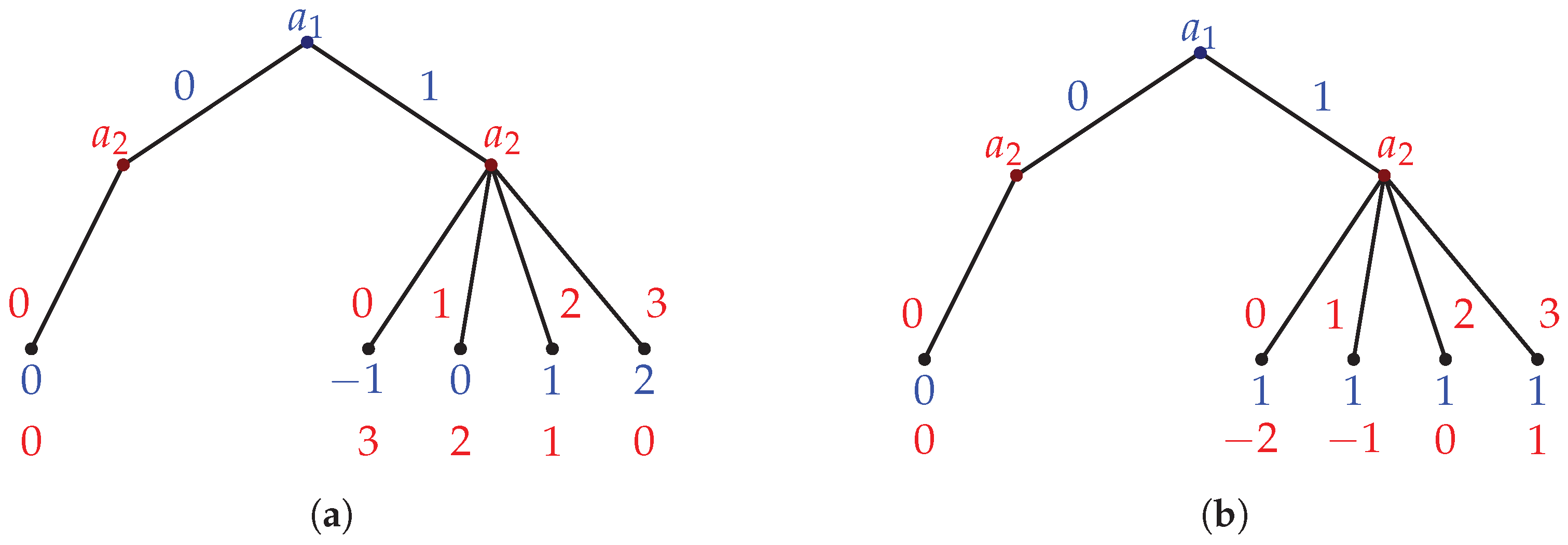
The Trust GameAssume a two-agent stage game $G_1$ in which $A_1=[0,1]$, $A_2=\left\{x\right|3y\ge x,y\in A_1\}$ and $u_1(y,x)=x-y$, $u_2(y,x)=3y-x$ for $y\in A_1$ and $x\in A_2$. By backward induction, when the first agent plays first, $(0,0)$ is the Nash equilibrium (NE). If, for the sake of illustration, we restrict Agent 1’s actions to $A_i^{\prime }=\{0,1\}$ for $i=1,2$, then Figure 5a shows the branches of the stage game where the two agents are named $a_1$ and $a_2$, respectively. As usual, the label on each edge is the action taken by the agent on the node above and, under each leaf, the first number is the utility of Agent 1 for the branch corresponding to the leaf and the second number is Agent 2’s utility.

Under the standard economic assumption of rational self-interest, the predicted actions of the first agent in the Trust Game will be to send nothing, and any behaviour that deviates from this self-interest is viewed as irrational. Since, in actual experiments, individuals significantly deviate from this NE, we argue that, as well as their material interest, they seek to build or protect their social reputation or their own ethical and pro-social values. We thus propose to develop a more realistic model of trust in economic behaviour by using a double game which includes the Trust Game above and a second social or conscience game as follows.

Example 6.

Double game for Trust GameLet $G_1$ be the Trust Game as in Example 5 and let $G_2$ be the associated conscience game in which $A_1=[0,1]$, $A_2=\left\{x\right|3y\ge x,y\in A_1\}$ and $u_1(y,x)=y$ and $u_2=x-2y$ for $y\in A_1$ and $x\in A_2$. By backward induction, $(1,3)$ is the NE. If again, we restrict Agent 1’s actions to $A_i^{\prime }=\{0,1\}$ for $i=1,2$, then Figure 5b shows the branches of the stage game. Consider a double game G with basic games $G_1$ and $G_2$ where $A_1=[0,1]$, $A_2=\left\{x\right|3y\ge x,y\in A_1\}$, ${\mathsf{\Theta }}_1=\{1/4\}$ and ${\mathsf{\Theta }}_2=\{0,2/3\}$. We have $U_1(y,x,1/4,2/3)=3/4x-1/2y$ and $U_2(y,x,1/4,2/3)=1/3x-1/3y$. Thus, $arg{max}_x{U}_2(y,x,1/4,2/3)=\left\{3y\right\}$. Put

$$\begin{array}{c}\hfill s_2\left({\theta }_2\right)=\left\{\begin{array}{cc}0& {\theta }_2=0\\ 3y& {\theta }_2=2/3\end{array}\right.\end{array}$$

Then, $U_1(y,0,1/4,{\theta }_2)=-y/2$ and $U_1(y,3y,1/4,{\theta }_2)=7y/4.$ Thus, $U_1(y,s_2\left({\theta }_2\right)\left(y\right))=p_0(-9y/4)+7y/4$. As a result,

$$\begin{array}{c}\hfill s_1(1/4)=arg\underset{y}{max}{U}_1(y,s_2\left({\theta }_2\right)\left(y\right))=\left\{\begin{array}{cc}1& p_0<7/9\\ y& p_0=7/9\\ 0& p_0>7/9\end{array}\right.\end{array}$$

Hence, $(s_1(1/4),s_2\left({\theta }_2\right))$ is a sub-game perfect equilibrium for the double game. We now see that, depending on its belief about Agent 2, Agent 1 can send any amount of money to Agent 2 and Agent 2 can return different amounts of money as an optimal solution for the trust double game.

8. Conclusions

We have shown that linear multidimensional Bayesian games are equivalent to uniform multigames, i.e., simultaneous competitions between the agents that play the same action in a finite number of basic games. Standard uniform multigames, where the action set of each agent consists of one NE inducing action per basic game, are proposed to model human rational-social decision making as in PD and the Trust Game and, more generally, for decision making by agents investing with their individual weights in multiple environments. We have proved that a standard uniform multigame has a compatible pure ex post NE if it has a pure ex post NE on its type profile space boundary and we have derived an algorithm, linear in the number of types, which checks if a compatible pure extreme types can be extended to the boundary.

We envisage applications of multigames for multi-agent systems in a variety of contexts. In addition, future work will consider extensions of the results in this paper to mixed ex post NE and extensions of multigames to the case for which the utilities of each agent depend affinely or piecewise affinely on its types and to the case when the utilities of each agent depend linearly or affinely on the types of all agents. A framework for implementing multigames in networks is also considered.

References

- Krishna, V.; Perry, M. Efficient Mechanism Design; Manuscript; Department of Economics, The Pennsylvania State University: University Park, PA, USA, 1998. [Google Scholar]
- Lucier, B.; Borodin, A. Price of anarchy for greedy auctions. In Proceedings of the Twenty-First Annual ACM-SIAM Symposium on Discrete Algorithms, Austin, TX, USA, 17–19 January 2010; SIAM: Philadelphia, PA, USA, 2010; pp. 537–553. [Google Scholar]
- Hartline, J.D. Bayesian mechanism design. Found. Trends Theor. Comput. Sci. 2013, 8, 143–263. [Google Scholar] [CrossRef]
- Hartline, J.D. Mechanism Design and Approximation Manuscript. 2017. Available online: http://jasonhartline.com/MDnA/ (accessed on 6 April 2018).
- Rabinovich, Z.; Naroditskiy, V.; Gerding, E.H.; Jennings, N.R. Computing pure bayesian-nash equilibria in games with finite actions and continuous types. Artif. Intell. 2013, 195, 106–139. [Google Scholar] [CrossRef]
- Edalat, A.; Ghoroghi, A.; Sakellariou, G. Multi-games and a double game extension of the prisoner’s dilemma. arXiv, 2012; arXiv:1205.4973. [Google Scholar]
- Ghoroghi, A. Multi-Games and Bayesian Nash Equilibriums. Ph.D. Thesis, Department of Computing, Imperial Collage London, London, UK, 2015. [Google Scholar]
- Harris, M.; Townsend, R.M. Resource allocation under asymmetric information. Econom. J. Econom. Soc. 1981, 49, 33–64. [Google Scholar] [CrossRef]
- Holmström, B.; Myerson, R.B. Efficient and durable decision rules with incomplete information. Econom. J. Econom. Soc. 1983, 51, 1799–1819. [Google Scholar] [CrossRef]
- Crémer, J.; McLean, R.P. Optimal selling strategies under uncertainty for a discriminating monopolist when demands are interdependent. Econom. J. Econom. Soc. 1985, 53, 345–361. [Google Scholar] [CrossRef]
- Bergemann, D.; Morris, S. Ex post implementation. Games Econ. Behav. 2008, 63, 527–566. [Google Scholar] [CrossRef]
- Bulow, J.I.; Geanakoplos, J.D.; Klemperer, P.D. Multimarket oligopoly: Strategic substitutes and complements. J. Political Econ. 1985, 93, 488–511. [Google Scholar] [CrossRef]
- Abolhassani, M.; Bateni, M.H.; Hajiaghayi, M.; Mahini, H.; Sawant, A. Network cournot competition. In Proceedings of the International Conference on Web and Internet Economics, Beijing, China, 14–17 December 2014; Springer: Cham, Switzerland, 2014; pp. 15–29. [Google Scholar]
- Bimpikis, K.; Ehsani, S.; Ilkilic, R. Cournot competition in networked markets. In Proceedings of the Fifteenth ACM Conference on Economics and Computation, Palo Alto, CA, USA, 8–12 June 2014; p. 733. [Google Scholar]
- Yanovskaya, E.B. Equilibrium points in polymatrix games. Litov. Mat. Sb. 1968, 8, 381–384. [Google Scholar]
- Kearns, M.; Littman, M.L.; Singh, S. Graphical models for game theory. In Proceedings of the Seventeenth Conference on Uncertainty in Artificial Intelligence, Seattle, WA, USA, 2–5 August 2001; Morgan Kaufmann Publishers Inc.: San Francisco, CA, USA, 2001; pp. 253–260. [Google Scholar]
- Papadimitriou, C.H.; Roughgarden, T. Computing correlated equilibria in multi-player games. J. ACM (JACM) 2008, 55, 14. [Google Scholar] [CrossRef]
- Ortiz, L.E.; Irfan, M.T. Tractable algorithms for approximate Nash equilibria in generalized graphical games with tree structure. In Proceedings of the Thirty-First AAAI Conference on Artificial Intelligence, San Francisco, CA, USA, 4–9 February 2017; pp. 635–641. [Google Scholar]
- Howson, J.T., Jr.; Rosenthal, R.W. Bayesian equilibria of finite two-person games with incomplete information. Manag. Sci. 1974, 21, 313–315. [Google Scholar] [CrossRef]
- Austrin, P.; Braverman, M.; Chlamtác, E. Inapproximability of NP-complete variants of Nash equilibrium. Theory Comput. 2013, 9, 117–142. [Google Scholar] [CrossRef]
- Rubinstein, A. Inapproximability of Nash equilibrium. In Proceedings of the Forty-Seventh Annual ACM Symposium On Theory of Computing, Portland, OR, USA, 14–17 June 2015; ACM: New York, NY, USA, 2015; pp. 409–418. [Google Scholar]
- Baumann, L. A Model of Weighted Network Formation. 2017. Available online: https://ssrn.com/abstract=2533533 (accessed on 16 July 2018).
- Damasio, A.; Tranel, D.; Damasio, H. Somatic markers and the guidance of behavior: Theory and preliminary testing. In Frontal Lobe Function and Dysfunction; Levin, H.S., Eisenberg, H.M., Benton, A.L., Eds.; Oxford University Press: New York, NY, USA, 1991. [Google Scholar]
- Bechara, A.; Damasio, H.; Damasio, A.R. Emotion, decision making and the orbitofrontal cortex. Cereb. Cortex 2000, 10, 295–307. [Google Scholar] [CrossRef] [PubMed]
- Loewenstein, G.; Lerner, J.S. The role of affect in decision making. Handb. Affect. Sci. 2003, 619, 3. [Google Scholar]
- Gintis, H. The Bounds of Reason: Game Theory and the Unification of the Behavioral Sciences; Princeton University Press: Princeton, NJ, USA, 2009. [Google Scholar]
- Ostrom, E. Biography of Robert Axelrod. PS Political Sci. Politics 2007, 40, 171–174. [Google Scholar] [CrossRef]
- Shubik, M. Game theory, behavior, and the paradox of the Prisoner’s Dilemma: Three solutions. J. Confl. Resolut. 1970, 14, 181–193. [Google Scholar] [CrossRef]
- Hausman, D.M. Taking the prisoner’s dilemma seriously: What can we learn from a trivial game? In The Prisoner’s Dilemma; Peterson, M., Ed.; Cambridge University Press: Cambridge, UK, 2015. [Google Scholar]
- Khadjavi, M.; Lange, A. Prisoners and their dilemma. J. Econ. Behav. Organ. 2013, 92, 163–175. [Google Scholar] [CrossRef]
- Brosig, J. Identifying cooperative behavior: Some experimental results in a Prisoner’s Dilemma game. J. Econom. Behav. Organ. 2002, 47, 275–290. [Google Scholar] [CrossRef]
- Berg, J.; Dickhaut, J.; McCabe, K. Trust, reciprocity, and social history. Games Econ. Behav. 1995, 10, 122–142. [Google Scholar] [CrossRef]
- Chaudhuri, A.; Gangadharan, L. An experimental analysis of trust and trustworthiness. South. Econ. J. 2007, 73, 959–985. [Google Scholar]
- Johnson, N.D.; Mislin, A.A. Trust games: A meta-analysis. J. Econ. Psychol. 2011, 32, 865–889. [Google Scholar] [CrossRef]
- Davis, J.B. Individuals and Identity in Economics; Cambridge University Press: Cambridge, UK, 2011. [Google Scholar]
- Fudenberg, D.; Tirole, J. Game Theory; The MIT Press: Cambridge, MA, USA, 1991. [Google Scholar]
- Devanur, N.; Hartline, J.D.; Karlin, A.; Nguyen, T. Prior-independent multi-parameter mechanism design. In Proceedings of the International Workshop on Internet and Network Economics, Singapore, 11–14 December 2011; Springer: Berlin/Heidelberg, Germany, 2011; pp. 122–133. [Google Scholar]
- Fu, H.; Hartline, J.D.; Hoy, D. Prior-independent auctions for risk-averse agents. In Proceedings of the Fourteenth ACM Conference on Electronic Commerce, Philadelphia, PA, USA, 16–20 June 2013; ACM: New York, NY, USA, 2013; pp. 471–488. [Google Scholar]
- Chen, P.-A.; De Keijzer, B.; Kempe, D.; Schäfer, G. The robust price of anarchy of altruistic games. In Proceedings of the International Workshop on Internet and Network Economics, Singapore, 11–14 December 2011; Springer: Berlin/Heidelberg, Germany, 2011; pp. 383–390. [Google Scholar]
- Axelrod, R.M. The Evolution of Cooperation; Basic Books: New York, NY, USA, 2006. [Google Scholar]
- Ounsley, J. The Prisoner’s Dilemma and Our Morals. Master’s Thesis, Department of Computing, Imperial Collage London, London, UK, 2010. [Google Scholar]
- McKelvey, R.D.; McLennan, A. Computation of equilibria in finite games. Handb. Comput. Econ. 1996, 1, 87–142. [Google Scholar]
Figure 1.
NEs in local games of three double games for PD, the shaded regions represent the continuous types: (a) , , with no pure ex post NE; (b) , , with one pure ex post NE; and (c) , with four pure ex post NEs.
Figure 2.
The partitioning of Θ in Example 3 into regions of constant local NE for G.
Figure 3.
The partition of the type space of Agent 2 for each extreme type of Agent 1 in the multigame of Example 4. The multigame has no compatible pure ex post NE by Theorem 2. The type shows that the partition of is not independent of .
Figure 4.
The partitioning of in a two-agent multigame with three games which shows that the multigame has a pure ex post NE. The types of each agent in the three partitioning of its type space are shown in three different colours.
Figure 5.
Trust Game (a); and Conscience Game (b).