Mean-Field Type Games between Two Players Driven by Backward Stochastic Differential Equations


Department of Mathematics, KTH Royal Institute of Technology, 100 44 Stockholm, Sweden
Games 2018, 9(4), 88; https://0-doi-org.brum.beds.ac.uk/10.3390/g9040088
Submission received: 3 September 2018
/
Revised: 16 October 2018
/
Accepted: 23 October 2018
/
Published: 1 November 2018
(This article belongs to the Special Issue Mean-Field-Type Game Theory)
Abstract
:In this paper, mean-field type games between two players with backward stochastic dynamics are defined and studied. They make up a class of non-zero-sum, non-cooperating, differential games where the players’ state dynamics solve backward stochastic differential equations (BSDE) that depend on the marginal distributions of player states. Players try to minimize their individual cost functionals, also depending on the marginal state distributions. Under some regularity conditions, we derive necessary and sufficient conditions for existence of Nash equilibria. Player behavior is illustrated by numerical examples, and is compared to a centrally planned solution where the social cost, the sum of player costs, is minimized. The inefficiency of a Nash equilibrium, compared to socially optimal behavior, is quantified by the so-called price of anarchy. Numerical simulations of the price of anarchy indicate how the improvement in social cost achievable by a central planner depends on problem parameters.
1. Introduction
Mean-field type games (MFTG) is a class of games in which payoffs and dynamics depend not only on the state and control profiles of the players, but also on the distribution of the state-control processes. MFTGs has by now a plethora of applications in the engineering sciences, see [1] and the references therein. This paper studies MFTGs between two players, with state-distribution dependent cost functionals , , and mean-field BSDE state dynamics. The Nash solution is dictated by the pair of inequalities
Following the path laid-out in [2], we establish a Pontryagin type maximum principle, yielding necessary and sufficient conditions for any pair of controls satisfying (1). Behavior in the equilibrium (1) is compared to the socially optimal solution, that minimizes the social cost
1.1. Related Work
Pontryagin’s maximum principle is the tool, alongside dynamic programming, to characterize optimal controls in both deterministic and stochastic settings. It can treat not only standard stochastic systems, but generalizes to optimal stopping, singular controls, risk-sensitive controls and partially observed models. Pontryagin’s maximum principle yields necessary conditions that must be satisfied by any optimal solution. The necessary conditions become sufficient under additional convexity conditions. Early results showed that an optimal control along with the corresponding optimal state trajectory must solve the so-called Hamiltonian system, which is a two-point (forward-backward) boundary value problem, together with a maximum condition of the so-called Hamiltonian function. A very useful aspect of this result is that minimization of the cost functional (over a set of control functions) may reduce to pointwise maximization of the Hamiltonian, at each point in time (over the set of control values). Pontryagin’s technique for deterministic systems and stochastic systems with uncontrolled diffusion can be summarized as follows: assume that there exists an optimal control, make a spike-variation of it and then consider the first order term of the Taylor expansion with respect to the perturbation. This leads to variational inequality and the result follows from duality. If the diffusion is controlled, second order terms in the Taylor expansion has to be considered. In this case, one ends up with two forward-backward SDEs and a more involved maximum condition for the Hamiltonian. See [3] for a detailed account. For stochastic systems, the backward equation is fundamentally different from the forward equation, whenever one is looking for adapted solutions. An adapted solution to a BSDE is a pair of adapted stochastic processes , where corrects “non-adaptiveness” caused by the terminal condition of . As pointed out by [4], the first component corresponds to the mean evolution of the dynamics, and to the risk between current time and terminal time. Linear BSDEs extends to non-linear BSDEs [5], with applications not only within stochastic optimal control but also in stochastic analysis [6] and finance [7,8], and to forward-backward SDEs (FBSDE). BSDEs with distribution-dependent coefficients, mean-field BSDEs, were derived as limits of particle systems in [9]. Existence and uniqueness results for mean-field BSDEs, as well as a comparison theorem, are provided in [10].
In stochastic differential games, both zero-sum and nonzero-sum, Pontryagin’s stochastic maximum principle (SMP) and dynamic programming are the main tools for obtaining conditions for an equilibrium. These tools were essentially inherited from the theory of stochastic optimal control. As in the optimal control setting, the latter deals with solving systems of second-order parabolic partial differential equations, while the former is related to analyzing FBSDEs where, in the case of initial state constraints, the BSDE corresponds to the adjoint process. For a recent example of the use of SMP in stochastic differential game theory, see [11].
The theory of mean-field type control (MFTC), initiated in [2], treats stochastic control problems with coefficients dependent on the marginal state-distribution. This theory is by now well developed for forward stochastic dynamics, i.e., with initial conditions on state [12,13,14,15]. With SMPs for MFTC problems at hand, MFTG theory can inherit these techniques like stochastic differential game theory does in the mean-field free case. See [16] for a review of solution approaches to MFTGs. A MFTC problem can be interpreted as a large population limit of a cooperative game, where the players share a joint goal to optimize some objective [17]. A close relative to MFTC is mean field games (MFG). MFGs is class of non-cooperative stochastic differential games where a large number of indistinguishable (anonymous) players interact weakly through a mean-field coupling term, initiated by [18,19] independently, and followed up by, among many others [20,21,22]. Weak player-to-player interaction through a mean-field coupling restricts the influence one player has on any other player to be inversely proportional to the number of players, hence the level of influence of any specific player is very small. The coupling of player state dynamics leads to conflicting objectives, and an approximation of mass behavior provides an approximate limit solution (equilibrium) to the MFG. In contrast to the MFG, players in a MFTG can be influential, and distinguishable (non-anonymous). That is, state dynamics and/or cost need not be of the same form over the whole player population, and a single player can have a major influence on other players’ dynamics and/or cost.
Already in [23], an SMP in local form was derived for a controlled non-linear BSDE. By first finding a global estimate for the variation of the second component of the BSDE solution, an SMP in global form was derived in [24]. A reinterpretation of BSDEs as forward stochastic optimal control problems [4] opened up for a new solution approach in the field of control of BSDEs. Inspired by the reinterpretation, optimal control of LQ BSDEs was solved in [25] by constructing a sequence of forward control problems with an additional state constraint, whose limit solution is the solution to the original LQ BSDE control problem. This approach was later used by [26] to solve a general FBSDE control problem, where the authors overcome the difficulty of controlling the diffusion in the forward process. Instead of writing down a second-order adjoint equation for the full system, the technique of [25] is used. Previous to that, [27] studied optimal control problem for general coupled forward–backward stochastic differential equations (FBSDEs) with controlled diffusions. A maximum principle of Pontryagin’s type for the optimal control is derived, by means of spike variation techniques.
Optimal control of mean-field BSDEs has recently gained attention. In [28] the mean-field LQ BSDE control problem with deterministic coefficients is studied. Assuming the control space is linear, linear perturbation is used to derive a stationarity condition which together with a mean-field FBSDE system characterizes the optimal control. Existence of optimal controls is also proven under convexity assumptions. Other recent work on the control of BSDEs includes [29,30], both using the FBSDE approach of [27].
1.2. Potential Applications of MFTG with Mean-Field BSDE Dynamics
In [31], a model is proposed for pedestrians groups moving towards targets they are forced to reach, such as deliveries and emergency personnel. The strict terminal condition leads to the formulation of a dynamic model for crowd motion where the state dynamics is a mean-field BSDE. Mean-field effects appear in pedestrian crowd models as approximations of aggregate human interaction, so the game would in fact be a MFTG [32]. A game between such groups is of interest since it can be a tool for decentralized decision making under conflicting interests. Other areas of application include strategies for financial investments, where often future conditions are specified [8,33] and lead to dynamic models including BSDEs. The already mentioned study [1] presents a lengthy list of applications of forward MFTGs in engineering sciences.
1.3. Paper Contribution and Outline
In this paper, control of mean-field BSDEs is extended to games between players whose state dynamics are mean-field BSDEs. Such games are in fact MFTGs, since the distribution of each player is effected by both players’ choice of strategy. Our MFTG could be viewed as a game between mean-field FBSDEs, where the backward equation is the state equation, and the forward equation is pure noise. A Pontryagin’s type SMP is derived, resulting in a verification theorem and conditions for existence of a Nash equilibrium. This solution approach is similar to that of [23,24,28]. The use of spike-perturbation requires minimal assumptions on the set of admissible controls, and differentiating measure-valued functions makes it possible to go beyond linear-quadratic mean-field cost and dynamics. The state BSDE is not converted to a forward optimization problem in the spirit of [25]. As a consequence, the adjoint equation in our SMP is a forward SDE. For the sake of comparison, optimality conditions for the cooperative situation are derived. In this setting, the players work together to optimize social cost, which is the the sum of player costs. The approach used is a straight-forward adaptation of the techniques used in control of SDEs of mean-field type; again, we do not need to take the route via some equivalent forward optimization problem to solve the backward MFTC problem. This cooperative game is a MFTC problem, and our result here is basically a special case of the FBSDE results in [27] or [26] mentioned above, although mean-field terms are present. Numerical simulations are done in the linear-quadratic case, which is explicitly solvable up to a system of ODEs. The examples pinpoint differences between player behavior in the game versus the centrally planned solution. The fraction between the social cost in the game equilibrium and the social cost optimum quantifies the game efficiency and was first studied in [34] for traffic coordination on networks under the name coordination ratio. This fraction was later renamed to the price of anarchy in [35]. We notice that paying a high price for using large control values, or deviating from a preferred initial position makes the problem stiffer, in the sense that the improvement by team optimality is decreasing, while paying a high price for mean-field related costs makes the problem less stiff.
The rest of this paper is organized as follows. The problem formulation is given in Section 2. Section 3 and Section 4 deal with necessary and sufficient conditions for any Nash equilibrium and social optimum; maximum principles for the MFTG and the MFTC are derived. An LQ problem is solved explicitly in Section 5, and numerical results are presented. The paper concludes with some remarks on possible extensions in Section 6, followed by an appendix containing proofs.
2. Problem Formulation
List of Symbols
- —the time horizon.
- —the underlying filtered probability space.
- —the distribution of a random variable X under .
- —the set of -valued -measurable random variables X such that .
- —the progressive -algebra.
- —a stochastic process .
- —the set of -valued, continuous -measurable processes such that .
- —the set of -valued -measurable processes such that .
- — the set of admissible controls for player i.
- —the set of probability measures on .
- —the set of probability measures on with finite second moment.
- —the t-marginal of the state-, law- and control-tuple of player i.
- —the trace (Frobenius) norm of the matrix Z.
- —derivative of the -valued function f.
- —derivative of the -valued function f, see Appendix A for details.
Let be a finite real number representing the time horizon of the game. Consider a filtered probability space on which two independent standard Brownian motions are defined, - and -dimensional respectively. Additionally, and , -measurable, are defined on the space. We assume that these five random objects are independent and that they generate the filtration . Notice that makes non-trivial. Let be the -algebra on of -progressively measurable sets. For , let be the set of -valued and continuous -measurable processes such that , and let be the set of -valued -measurable processes such that .
Let be a separable metric space, . Player i picks her control from the set
The distribution of any random variable will be denoted by , and will denote the index . Given a pair of controls , consider the system of controlled BSDEs
where and . Furthermore,
where is equipped with the norm , being the 2-Wasserstein metric on . is equipped with the trace norm . Note that if X is a square integrable random variable in , then and , the space of measures with finite -norm.
Given , a pair of -valued -measurable processes , , is a solution to (4) if
and .
Remark 1.
Any terminal condition naturally induces a -martingale . The martingale representation theorem then gives existence of a unique process such that , i.e., plays the role of the projection and without it, would not be -measurable. Hence the noise generating the filtration is common to both players, and , is their respective reaction to it. Player i may actually be effected by all the noise in the filtration even if only some components of appear in . An interpretation of is that it is a second control of player i: first she plays to heed preferences on energy use, initial position etc., then she picks so that her path to is the optimal prediction based on available information in the filtration at any given time. The component in (4) acts as a velocity in.
Existence and uniqueness of (4) is given by a slight variation of the results of [10], where the one-dimensional case is treated. For the d-dimensional mean-field free case, see [36].
Assumption 1.
The process , , belongs to and for any , , , is -measurable.
Assumption 2.
Given a pair of control values , there exists a constant such that for all and tuples
Theorem 1.
Let Assumptions 1 and 2 hold. Then, for any terminal conditions and , the system of mean-field BSDEs (4) has a unique solution , .
Next, we introduce the best reply of player i as follows:
for given maps and .
Assumption 3.
For any pair of controls , and .
The problems we consider next are
- The Mean-field Type Game (MFTG): find the Nash equilibrium controls of
- The Mean-field Type Control Problem (MFTC): find the optimal control pair of
In the game each player assumes that the other player acts rationally, i.e., minimizes cost, and picks her control as the best response to that. This leads to a set of two inequalities, characterizing any control pair that constitute a Nash equilibrium. In this paper, each player is aware of the other player’s control set, best response function and state dynamics. Therefore, even though the decision process is decentralized, both players solve the same set of inequalities. When there is not a unique Nash equilibrium, there is an ambiguity around which equilibrium strategy to play if the players do not communicate. In the control problem, a central planner decides what strategies are played by both of the players. The central planner might just be the two players cooperating towards a common goal, or some superior decision maker. The goal is to find the control pair that minimizes the social cost J. This notion of a centrally planned/cooperative solution is related to the concept of team optimality in team problems [37]. In a team problem, the players share a common objective. A team-optimal solution is then the solution to the joint minimization of the common objective. In our case, the social cost J is a common objective in the MFTC. The Nash solution to the team problem is given by the control pair that satisfies the two inequalities
In (11), each player is minimizing the social cost with respect to its marginal, under the assumption that the other player is minimizing its marginal. This is the so-called player-by-player optimality of a control pair in a team problem. Notice that if we set in (9), it becomes a team problem. The solution to the MFTG (9) will then be the player-by-player optimal solution to the minimization of the social cost.
Logically, we expect the optimal social cost to be lower than the social cost in a Nash equilibrium. The ratio between the worst case social cost in the game and the optimal social cost is called the price of anarchy, and we will highlight it in the numerical simulations in Section 5 where we also observe behavioral differences between MFTG and MFTC given identical data.
3. Problem 1: MFTG
This section is the derivation of necessary and sufficient equilibrium conditions of (9). Given the existence of such a pair of controls, we derive the conditions by the means of a Pontryagin type stochastic maximum principle.
Assume that is a Nash equilibrium for the MFTG, i.e., satisfies the following system of inequalities,
Consider the first inequality, with chosen as a spike-perturbation of . That is, for ,
Here, is any subset of of Lebesgue measure . Clearly, . When player 1 plays the spike-perturbed control and player 2 plays the equilibrium control , we denote the dynamics by
The performance of the perturbed dynamics (14) will be compared with that of the equilibrium dynamics
For simplicity, we write for , , ,
In this shorthand notation, which will be used from now on, the difference in performance is
Any derivative of will be denoted , indifferent of the space the function is mapping from/to.
Assumption 4.
The functions
are for all t a.s. differentiable at , and respectively. Furthermore,
are for all t a.s. uniformly bounded, and
For ,
A brief overview on differentiation of -valued functions is found in Appendix A, and the notation is defined in (A8). Both and appear in (21), this suggests that we need to introduce two first order variation processes. That is, we want , that for some satisfies
Let denote variation in so that for ,
Assumption 5.
For , , and , there exists a constant such that
a.s. for all .
Lemma 1.
Let Assumptions 1, 2, 4 and 5 be in force. The first order variation processes that satisfy (22) is given by the following system of BSDEs,
A proof is found in the appendix. By Lemma 1,
where the introduced costates , , satisfy . The notation is defined in (A10). Assumption 4 grants us existence and uniqueness to Equation (27) below.
Lemma 2 (Duality relation).
Lett Assumptions 1, 2 and 4 hold. Let be the solution to the SDE
where for , , and ,
Then the following duality relation holds,
A proof of the lemma above is found in the appendix. We have that
Therefore
From the last identity, we can derive necessary and sufficient conditions for player 1’s best response to .
The same argument can be carried out for players 2’s best response to . Naturally, we need to impose the corresponding assumptions on player 2’s control. For completeness and later reference, we state now the second player’s version of Lemma 2.
Lemma 3 (Duality relation, player 2).
Let Assumptions 1, 2 and 4 hold, and let be the solution to the SDE
where for , , and ,
Then the following duality relation holds,
Necessary equilibrium conditions can be stated as a system of 6 Equations, 2 state BSDEs and 4 costate (adjoint) SDEs. Sufficient conditions for a Nash equilibrium can now be stated as convexity conditions on the 4 functions . We let Assumptions 1–5 be in place.
Theorem 2.
Proof.
Let , and for . Consider the spike-perturbation
Then
Applying (33), we obtain
Sending ε to zero yields
The last inequality holds for all , thus
By measurability of the integrand in (42),
The same argument yields
□
Theorem 3.
[Sufficient equilibrium conditions] Suppose that and satisfy (37). Suppose furthermore that for , ,
is concave a.s. and
is convex a.s. Then constitute an equilibrium control and , , is an equilibrium for the MFTG.
Proof.
By assumption, for any spike variation, almost surely for a.e. t. Applying the convexity and concavity assumptions in the expansion steps results in the inequality
□
4. Problem 2: MFTC
Carrying out a similar argument to that of the previous section, we find necessary optimality conditions for problem (10). Also, we readily get a verification theorem. The pair is optimal if
Assume from now on that is an optimal control. We study the inequality (48) when is a spike-perturbation of ,
where is any subset of of Lebesgue measure ε and . When the players use the perturbed control, we denote the state dynamics by
and we will compare their performance to that of the optimally controlled state dynamics
For simplicity, we write for ,
and in this notation,
where and . Again, we want to find first order variation processes , that satisfy (22) with replaced by its ’checked’ counterpart .
Assumption 6.
The functions
are for all t a.s. differentiable at , and respectively. Furthermore,
are for all t a.s. uniformly bounded and .
Notice that the point of differentiability is generally not the same in Assumptions 4 and 6. Above, is an optimal control while in Assumption 4, it is an equilibrium control. Let δ denote simultaneous variation in controls, for ,
Lemma 4.
Let Assumptions 1, 2, 5 and 6 be in force. The first order variation processes that satisfy the ’checked’ version of (22) is given by the following system of BSDEs,
The proof follows the same steps as the proof of Lemma 1.
By Lemma 4,
where .
Lemma 5 (Duality relation).
Let Assumptions 1, 2 and 6 hold. Let be the solution to the SDE
where for , , and (,
Then the following duality relation holds,
The proof of Lemma 5 is almost identical that of Lemma 2. By Lemma 4,
Thus
In the following two theorems, Assumptions 1–3, 5 and 6 are in force.
Theorem 4 (Necessary optimality conditions).
Theorem 5 (Sufficient optimality conditions).
Suppose satisfy (64). Suppose furthermore that for , ,
is concave a.s. and
is convex a.s. Then is an optimal control and , solves the MFTC.
5. Example: The Linear-Quadratic Case
In this section we consider a linear-quadratic version of (9) and (10), in the one dimensional case. Let , be deterministic coefficient functions, uniformly bounded over . Additionally, for . Define
The uniform boundedness of the coefficients implies Assumptions 1–6, given initial costs , satisfying Assumption 4 and 6. Assumption 3 (integrability of ) follows by classical BSDE estimates [38]. Recall player 1 and 2’s Hamiltonian, defined in (28) and (35). In the setup of this example,
The Hessian of is
and the Hessian of is
The coefficients are further assumed to be such that and are negative semi-definite for all . Also, we assume that , yet unspecified, is convex. Theorem 3 yields
where solves (27) or (34), depending on i. In fact the equilibrium is unique in this case, since is the unique pointwise solution to (37) and is unique, see (A25) and (A26). By Theorem 5,
where solves (59), is an optimal control for the linear-quadratic MFTC and it is unique.
5.1. MFTG
The equilibrium dynamics are
We see that only two costate processes, and , are relevant here. This is a consequence of the lack of explicit dependence on in the and specified in (67). Nevertheless, the running cost depends implicitly on through player ’s state and mean.
We make the following ansatz: there exists deterministic functions , and , , such that
Clearly, we need to impose the terminal conditions
Calculations presented in the appendix identifies coefficients and yields the following system of ODEs determining ,
where
5.2. MFTC
The optimally controlled dynamics are
We make almost the same ansatz as before, assume that there exists deterministic functions , and , , with terminal conditions
such that
5.3. Simulation and the Price of Anarchy
Let , be preferred initial positions for player 1 and 2 respectively, and
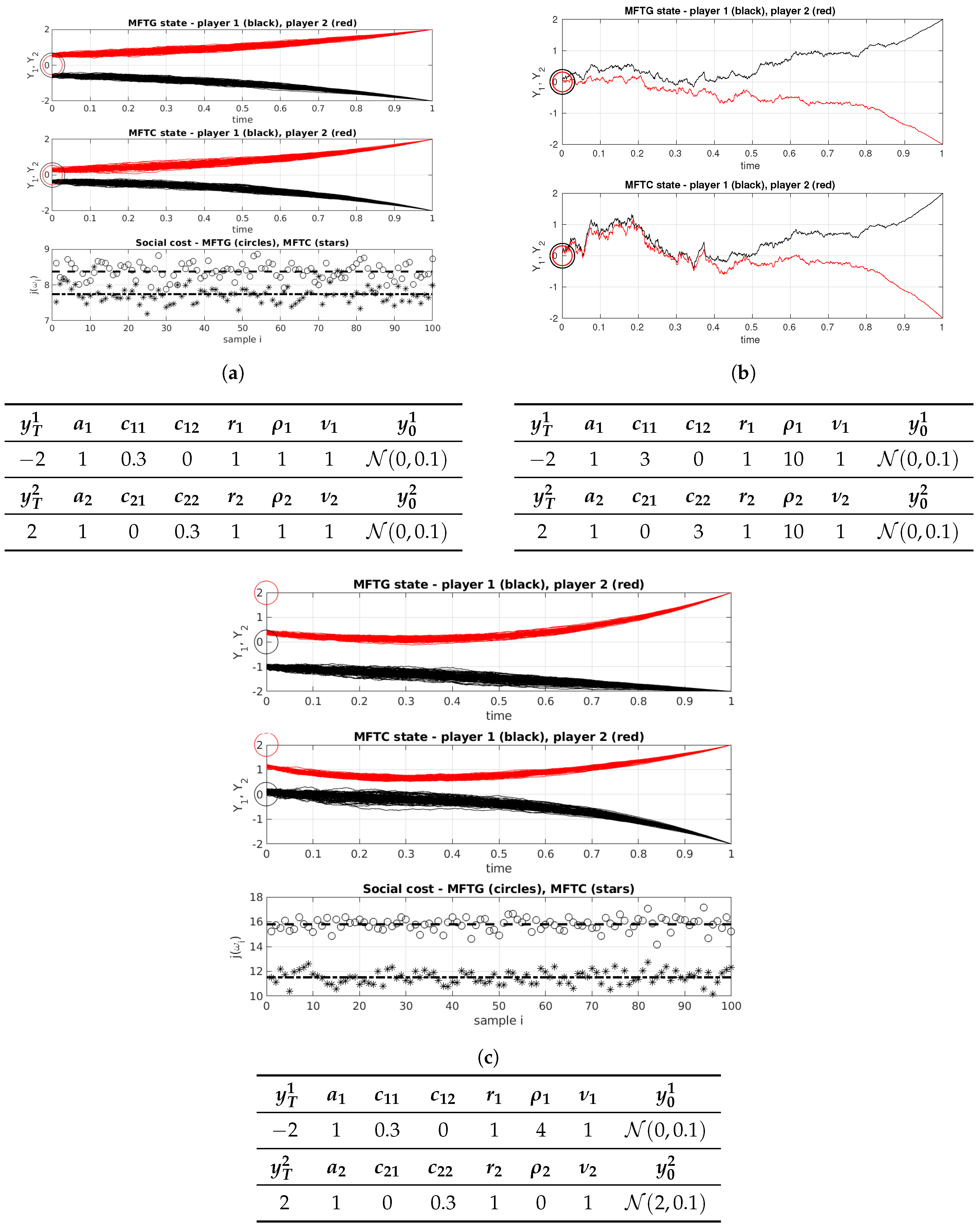
In this setup, and are negative semi-definite if , is convex if . In Figure 1 numerical simulations of MFTG and MFTC are presented. In (a), the two players have identical preferences, but different terminal conditions. The situation is symmetric in the sense that we expect the realized paths of player 1 reflected through the line to be approximately paths of player 2. In (c), preferences are asymmetric and as a consequence, the realized paths are not each others mirrored images.
The central planner in a MFTC uses more information than a single player does. In fact, in our example, when in the MFTG. The interpretation is that in the game, player i does not care about player ’s noise, only its mean state. For the central planner however, is not identically zero for . This can be observed in (b), where the central planner makes the player states evolve under some common noise.
In (c) we see an interesting contrast between the MFTG and the MFTC. Player 1 (black) feels no attraction to player 2 () while player 2 is attracted to the mean position of player 1 (). In the game, player 1 travels on the straight line from to its terminal position . Player 2, on the other hand, deviates far from its preferred initial position at time , only to be in the proximity of player 1. In the MFTC, the central planner makes player 1 linger around for some time, before turning south towards the terminal position. The result is less movement movement by player 2. Even though player 1 pays a higher individual cost, the social cost is reduced by approximately . The social cost J is approximated by
where . In (a) and (c), the outcomes of j (circles for equilibrium control, stars for optimal control) are presented along with the approximation of J (dashed lines) for . The optimal control yields the lower social cost in both cases. This is expected, the general inefficiency of a Nash equilibrium in nonzero-sum games is well known [39]. The price of anarchy quantifies the inefficiency due to non-cooperation, see for static games [34,40], for differential games [41] and for linear-quadratic mean-field type games [42]. The price of anarchy in mean-field games has been studied recently in [43,44]. It is defined as the largest ratio between social cost for an equilibrium (MFTG) to the optimal social cost (MFTC),
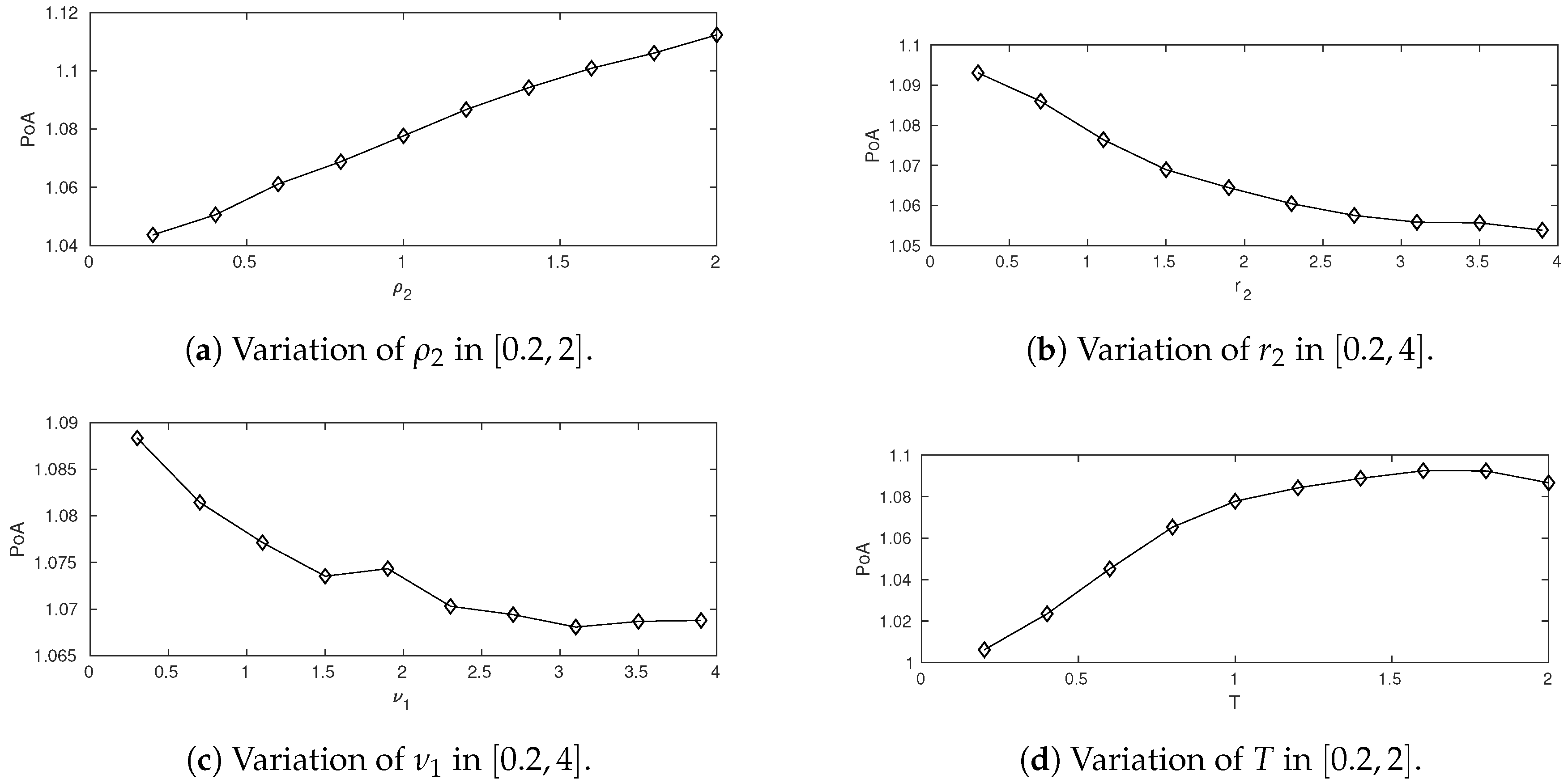
Taking the parameter set of (a) as a point of reference, see Table 1, we vary one parameter at the time and study . The result is presented in Figure 2. In the intervals studied, is increasing in and T and decreasing in and . The reason is that the players become less flexible when and/or are increased, and the improvement a central planner can do decreases. On the other hand, an increased time horizon gives the central planner more time to improve the social cost. Also, an increased preference on attraction rewards the unegoistic behavior in the MFTC model.
6. Conclusions and Discussion
Mean-field type games with backward stochastic dynamics, where the coefficients are allowed to depend on the marginal distributions of the player states, have been defined in this paper. Under regularity assumptions necessary conditions for a Nash equilibrium have been derived in the form of a stochastic maximum principle. Additional convexity assumptions yielded sufficient conditions. In linear-quadric examples, player behavior in the MFTG is compared to the centrally planned solution in the MFTC. The efficiency of the MFTG Nash equilibrium, quantified by the price of anarchy, and its dependence on problem parameters is studied.
The framework presented in this paper has many possible extensions, towards both theory and applications. The theory for martingale-driven BSDEs is now standard, and one could exchange throughout this paper for two martingales , possibly jump processes, and approach the game with the theory of forward-backward SDEs. Indeed, the topic of games between mean-field FBSDEs seems yet unexplored. These kind of problems would have immediate applications in finance.
With our definition of , we have restricted ourselves to open loop adapted controls in this paper. Other information structures, such as perfect/partial state- and/or law feedback controls, lagged or noise-perturbed controls are possible. Furthermore, both players have perfect information about each other in this paper. Taking inspiration from for example [45,46], the access to information could be restricted, so that the players have only partial information on states/laws. These types of extensions are interesting both from the theoretical and applied point of view. Depending on application, the information structure of the problem will naturally change.
Acknowledgments
Financial support from the Swedish Research Council (2016-04086) is gratefully acknowledged. The author would like to thank Boualem Djehiche and Salah Choutri for fruitful discussions and useful suggestions, and the anonymous reviewers, whose remarks helped to substantially improve this work.
Conflicts of Interest
The author declares no conflict of interest.
Abbreviations
The following abbreviations are used in this manuscript:
| BSDE | Backward stochastic differential equation |
| FBSDE | Forward-backward stochastic differential equation |
| LQ | Linear-quadratic |
| MFTC | Mean-field type control problem |
| MFTG | Mean-field type game |
| ODE | Ordinary differential equation |
| PoA | Price of Anarchy |
| SDE | Stochastic differential equation |
Appendix A. Differentiation and Approximation of Measure-Valued Functions
Derivatives of measure-valued functions will be defined with the lifting technique, outlined for example in [14,15,50]. Consider the function . We assume that our probability space is rich enough, so that for every , there exists a square-integrable random variable X whose distribution is μ, i.e., . For example, has this property. Then we may write and we can differentiate F in Fréchet-sense whenever there exists a continuous linear functional such that
where . is the Fréchet derivative of f at μ, in the direction Y and we have that
By Riesz’ Representation Theorem, is unique and it is known [14] that there exists a Borel function , independent of the version of X, such that . Therefore, with for some random variable , (A1) can be written as
We denote , , and we have the identity
Example A1.
If then
and .
Example A2.
If then .
The Taylor approximation of a measure-valued function is given by (A3), and we will write
Assume now that f takes another argument, ξ. Then
where the expectation is not taken over the tilded variable. Note that is deterministic. In situations where the expected value is taken only over the directional argument of , we will write
The expected value in (A7) is a random quantity because of . Taking another expected value, and changing the order of integration, leads to
where the tilded expectation is taken only over the tilded variable. The notation for this will be
Appendix B. Proofs
Lemma 1
Let
then . An application of Ito’s formula to yields
Let D denote the largest bound for all the derivatives of and present. By Jensen’s and Young’s inequalities,
The stochastic integrals in (A12) are local martingales and vanish under an expectation [36]. Therefore, with ,
Let , then
and by Hölder’s and Young’s inequalities,
By Assumption 5 and the definition of , we have for some ,
For , we conclude that
where depends on δ, the bound D, the Lipschitz coefficient of and the integration bound in the definition of . The steps above can be repeated for the intervals , , etc. until 0 is reached. After a finite number of iterations, we have
where depends on and T. This is the first estimate in (22). The second estimate follows from similar calculations.
Lemma 2
Integration by parts yields
Assume that , then
Hence, the lemma is equivalent to that, under expectations, we have
We match coefficients and get
Linear-Quadratic MFTG–Derivation of ODE System
Under the ansatz, the adjoint equation is
and the expected value of solves
The initial conditions are given by a system of linear equations, which is derived is the same way as (A25) and (A26). Applying Ito’s formula to the ansatz, and using (A25) and (A26), we get
We can now match these dynamics with the true state dynamics and we get the system of ODEs (76) and .
References
- Djehiche, B.; Tcheukam, A.; Tembine, H. Mean-Field-Type Games in Engineering. AIMS Electron. Electr. Eng. 2017, 1, 18–73. [Google Scholar] [CrossRef]
- Andersson, D.; Djehiche, B. A maximum principle for SDEs of mean-field type. Appl. Math. Optim. 2011, 63, 341–356. [Google Scholar] [CrossRef]
- Yong, J.; Zhou, X.Y. Stochastic Controls: Hamiltonian Systems and HJB Equations; Springer Science & Business Media: Berlin, Gremany, 1999; Volume 43. [Google Scholar]
- Kohlmann, M.; Zhou, X.Y. Relationship between backward stochastic differential equations and stochastic controls: A linear-quadratic approach. SIAM J. Control Optim. 2000, 38, 1392–1407. [Google Scholar] [CrossRef]
- Pardoux, É.; Peng, S. Adapted solution of a backward stochastic differential equation. Syst. Control Lett. 1990, 14, 55–61. [Google Scholar] [CrossRef]
- Peng, S. Probabilistic interpretation for systems of quasilinear parabolic partial differential equations. Stoch. Stoch. Rep. 1991, 37, 61–74. [Google Scholar] [CrossRef]
- Duffie, D.; Epstein, L.G. Stochastic differential utility. Econom. J. Econom. Soc. 1992, 60, 353–394. [Google Scholar] [CrossRef]
- El Karoui, N.; Peng, S.; Quenez, M.C. Backward stochastic differential equations in finance. Math. Financ. 1997, 7, 1–71. [Google Scholar] [CrossRef]
- Buckdahn, R.; Djehiche, B.; Li, J.; Peng, S. Mean-field backward stochastic differential equations: A limit approach. Ann. Probab. 2009, 37, 1524–1565. [Google Scholar] [CrossRef]
- Buckdahn, R.; Li, J.; Peng, S. Mean-field backward stochastic differential equations and related partial differential equations. Stoch. Process. Appl. 2009, 119, 3133–3154. [Google Scholar] [CrossRef]
- Moon, J.; Duncan, T.E.; Basar, T. Risk-Sensitive Zero-Sum Differential Games. IEEE Trans. Autom. Control 2018, in press. [Google Scholar] [CrossRef]
- Bensoussan, A.; Frehse, J.; Yam, P. Mean Field Games and Mean Field Type Control Theory; Springer: Berlin, Germany, 2013; Volume 101. [Google Scholar]
- Djehiche, B.; Tembine, H.; Tempone, R. A stochastic maximum principle for risk-sensitive mean-field type control. IEEE Trans. Autom. Control 2015, 60, 2640–2649. [Google Scholar] [CrossRef]
- Buckdahn, R.; Li, J.; Ma, J. A Stochastic Maximum Principle for General Mean-Field Systems. Appl. Math. Optim. 2016, 74, 507–534. [Google Scholar] [CrossRef]
- Carmona, R.; Delarue, F. Probabilistic Theory of Mean Field Games with Applications I–II; Springer: Berlin, Germany, 2018. [Google Scholar]
- Tembine, H. Mean-field-type games. AIMS Math. 2017, 2, 706–735. [Google Scholar] [CrossRef]
- Lacker, D. Limit Theory for Controlled McKean–Vlasov Dynamics. SIAM J. Control Optim. 2017, 55, 1641–1672. [Google Scholar] [CrossRef]
- Huang, M.; Malhamé, R.P.; Caines, P.E. Large population stochastic dynamic games: Closed-loop McKean-Vlasov systems and the Nash certainty equivalence principle. Commun. Inf. Syst. 2006, 6, 221–252. [Google Scholar]
- Lasry, J.M.; Lions, P.L. Mean field games. Jpn. J. Math. 2007, 2, 229–260. [Google Scholar] [CrossRef]
- Li, T.; Zhang, J.F. Asymptotically optimal decentralized control for large population stochastic multiagent systems. IEEE Trans. Autom. Control 2008, 53, 1643–1660. [Google Scholar] [CrossRef]
- Tembine, H.; Zhu, Q.; Başar, T. Risk-sensitive mean-field games. IEEE Trans. Autom. Control 2014, 59, 835–850. [Google Scholar] [CrossRef]
- Moon, J.; Basar, T. Linear Quadratic Risk-Sensitive and Robust Mean Field Games. IEEE Trans. Automat. Contr. 2017, 62, 1062–1077. [Google Scholar] [CrossRef]
- Peng, S. Backward stochastic differential equations and applications to optimal control. Appl. Math. Optim. 1993, 27, 125–144. [Google Scholar] [CrossRef]
- Dokuchaev, N.; Zhou, X.Y. Stochastic controls with terminal contingent conditions. J. Math. Anal. Appl. 1999, 238, 143–165. [Google Scholar] [CrossRef]
- Lim, A.E.; Zhou, X.Y. Linear-quadratic control of backward stochastic differential equations. SIAM J. Control Optim. 2001, 40, 450–474. [Google Scholar] [CrossRef]
- Wu, Z. A general maximum principle for optimal control of forward–backward stochastic systems. Automatica 2013, 49, 1473–1480. [Google Scholar] [CrossRef]
- Yong, J. Forward-backward stochastic differential equations with mixed initial-terminal conditions. Trans. Am. Math. Soc. 2010, 362, 1047–1096. [Google Scholar] [CrossRef]
- Li, X.; Sun, J.; Xiong, J. Linear Quadratic Optimal Control Problems for Mean-Field Backward Stochastic Differential Equations. Appl. Math. Optim. 2016, 1–28. [Google Scholar] [CrossRef]
- Tang, M.; Meng, Q. Linear-Quadratic Optimal Control Problems for Mean-Field Backward Stochastic Differential Equations with Jumps. arXiv, 2016; arXiv:1611.06434. [Google Scholar]
- Li, J.; Min, H. Controlled mean-field backward stochastic differential equations with jumps involving the value function. J. Syst. Sci. Complex. 2016, 29, 1238–1268. [Google Scholar] [CrossRef]
- Aurell, A.; Djehiche, B. Modeling tagged pedestrian motion: A mean-field type control approach. arXiv, 2018; arXiv:1801.08777. [Google Scholar]
- Aurell, A.; Djehiche, B. Mean-field type modeling of nonlocal crowd aversion in pedestrian crowd dynamics. SIAM J. Control Optim. 2018, 56, 434–455. [Google Scholar] [CrossRef]
- Chen, Z.; Epstein, L. Ambiguity, risk, and asset returns in continuous time. Econometrica 2002, 70, 1403–1443. [Google Scholar] [CrossRef]
- Koutsoupias, E.; Papadimitriou, C. Worst-case equilibria. In Annual Symposium on Theoretical Aspects of Computer Science; Springer: Berlin, Germany, 1999; pp. 404–413. [Google Scholar]
- Papadimitriou, C. Algorithms, games, and the internet. In Proceedings of the Thirty-Third Annual ACM Symposium on Theory of Computing, Crete, Greece, 6–8 July 2001; pp. 749–753. [Google Scholar]
- Pardoux, É. BSDEs, weak convergence and homogenization of semilinear PDEs. In Nonlinear Analysis, Differential Equations and Control; Springer: Berlin, Germany, 1999; pp. 503–549. [Google Scholar]
- Basar, T.; Olsder, G.J. Dynamic Noncooperative Game Theory; Society for Industrial and Applied Mathematics: Philadelphia, PA, USA, 1999; Volume 23. [Google Scholar]
- Zhang, J. Backward Stochastic Differential Equations: From Linear to Fully Nonlinear Theory; Springer: Berlin, Germany, 2017; Volume 86. [Google Scholar]
- Dubey, P. Inefficiency of Nash equilibria. Math. Oper. Res. 1986, 11, 1–8. [Google Scholar] [CrossRef]
- Koutsoupias, E.; Papadimitriou, C. Worst-case equilibria. Comput. Sci. Rev. 2009, 3, 65–69. [Google Scholar] [CrossRef]
- Başar, T.; Zhu, Q. Prices of anarchy, information, and cooperation in differential games. Dyn. Games Appl. 2011, 1, 50–73. [Google Scholar] [CrossRef]
- Duncan, T.E.; Tembine, H. Linear–Quadratic Mean-Field-Type Games: A Direct Method. Games 2018, 9, 7. [Google Scholar] [CrossRef]
- Carmona, R.; Graves, C.V.; Tan, Z. Price of anarchy for mean field games. arXiv, 2018; arXiv:1802.04644. [Google Scholar]
- Cardaliaguet, P.; Rainer, C. On the (in) efficiency of MFG equilibria. arXiv, 2018; arXiv:1802.06637. [Google Scholar]
- Ma, H.; Liu, B. Maximum principle for partially observed risk-sensitive optimal control problems of mean-field type. Eur. J. Control 2016, 32, 16–23. [Google Scholar] [CrossRef]
- Ma, H.; Liu, B. Linear-quadratic optimal control problem for partially observed forward-backward stochastic differential equations of mean-field type. Asian J. Control 2016, 18, 2146–2157. [Google Scholar] [CrossRef]
- Semasinghe, P.; Maghsudi, S.; Hossain, E. Game theoretic mechanisms for resource management in massive wireless IoT systems. IEEE Commun. Mag. 2017, 55, 121–127. [Google Scholar] [CrossRef]
- Tsiropoulou, E.E.; Vamvakas, P.; Papavassiliou, S. Joint customized price and power control for energy-efficient multi-service wireless networks via S-modular theory. IEEE Trans. Green Commun. Netw. 2017, 1, 17–28. [Google Scholar] [CrossRef]
- Katsinis, G.; Tsiropoulou, E.E.; Papavassiliou, S. Multicell Interference Management in Device to Device Underlay Cellular Networks. Future Internet 2017, 9, 44. [Google Scholar] [CrossRef]
- Cardaliaguet, P. Notes on Mean Field Games. Technical Report. 2010. Available online: https://www.researchgate.net/publication/228702832 (accessed on 3 September 2018).
Figure 1.
Numerical examples: (a) symmetric preference, (b) single path sample, (c) asymmetric attraction and initial position. Circles indicate the preferred initial positions.
Figure 1.
Numerical examples: (a) symmetric preference, (b) single path sample, (c) asymmetric attraction and initial position. Circles indicate the preferred initial positions.

Figure 2.
Numerical approximations (N = 5000) of the price of anarchy PoA.


Table 1.
Parameter values in the symmetric case (a).
| −2 | 1 | 0.3 | 0 | 1 | 1 | 1 | |
| 2 | 1 | 0 | 0.3 | 1 | 1 | 1 |
© 2018 by the author. Licensee MDPI, Basel, Switzerland. This article is an open access article distributed under the terms and conditions of the Creative Commons Attribution (CC BY) license (http://creativecommons.org/licenses/by/4.0/).
Share and Cite
MDPI and ACS Style
Aurell, A. Mean-Field Type Games between Two Players Driven by Backward Stochastic Differential Equations. Games 2018, 9, 88. https://0-doi-org.brum.beds.ac.uk/10.3390/g9040088
AMA Style
Aurell A. Mean-Field Type Games between Two Players Driven by Backward Stochastic Differential Equations. Games. 2018; 9(4):88. https://0-doi-org.brum.beds.ac.uk/10.3390/g9040088
Chicago/Turabian StyleAurell, Alexander. 2018. "Mean-Field Type Games between Two Players Driven by Backward Stochastic Differential Equations" Games 9, no. 4: 88. https://0-doi-org.brum.beds.ac.uk/10.3390/g9040088
Note that from the first issue of 2016, this journal uses article numbers instead of page numbers. See further details here.