Article

Evaluation of Flow Resistance Models Based on Field Experiments in a Partly Vegetated Reclamation Channel

by
Giuseppe Francesco Cesare Lama
1,*,
Alessandro Errico
2,
Simona Francalanci
3,
Luca Solari
3,
Federico Preti
2 and
Giovanni Battista Chirico
1
1
Department of Agricultural Sciences, Water Resources Management and Biosystems Engineering Division, University of Naples Federico II, 80055 Portici (NA), Italy
2
Department of Agricultural, Food, Environmental and Forestry Sciences and Technologies, University of Florence, 50144 Firenze, Italy
3
Department of Civil and Environmental Engineering, University of Florence, 50139 Firenze, Italy
*
Author to whom correspondence should be addressed.
Submission received: 6 January 2020 / Revised: 20 January 2020 / Accepted: 24 January 2020 / Published: 25 January 2020

Abstract

:
This study presents a methodology for improving the efficiency of Baptist and Stone and Shen models in predicting the global water flow resistance of a reclamation channel partly vegetated by rigid and emergent riparian plants. The results of the two resistance models are compared with the measurements collected during an experimental campaign conducted in a reclamation channel colonized by Common reed (Phragmites australis (Cav.) Trin. ex Steud.). Experimental vegetative Chézy’s flow resistance coefficients have been retrieved from the analysis of instantaneous flow velocity measurements, acquired by means of a downlooking 3-component acoustic Doppler velocimeter (ADV) located at the channel upstream cross section, and by water level measurements obtained through four piezometers distributed along the reclamation channel. The main morphometrical vegetation features (i.e., stem diameters and heights, and bed surface density) have been measured at six cross sections of the vegetated reclamation channel. Following the theoretical assumptions of the divided channel method (DCM), three sub-sections have been delineated in the reference cross section to represent the impact of the partial vegetation cover on the cross sectional variability of the flow field, as observed with the ADV measurements. The global vegetative Chézy’s flow resistance coefficients have been then computed by combining each resistance model with four different composite cross section methods, respectively suggested by Colebatch, Horton, Pavlovskii, and Yen. The comparative analysis between the modeled and the experimental vegetative Chézy’s coefficients has been performed by computing the relative prediction error (εr, expressed in %) under two flow rate regimes. Stone and Shen model combined with the Horton composite cross section method provides vegetative Chézy’s coefficients with the lowest εr.

1. Introduction

The presence of backwater in manmade reclamation channels enhances the growth of riparian vegetation, promoting the expansion of aquatic and terrestrial habitats and improving water quality [1,2]. In this context, the analysis of the real-scale interaction between riparian plants and water flow in vegetated channels can provide relevant hints to the administrators of land reclamation areas, about the most useful approaches to be followed when managing the riparian vegetation, which can ensure the conveyance capacity of the channel with limited impacts on the natural habitats [1].
One of the most challenging tasks when programming the management of riparian vegetation in reclamation channels is the definition of simple and accurate models for assessing the global flow resistance coefficients (e.g., the vegetative Chèzy flow resistance coefficient Cr [3,4], the Manning’s n hydraulic roughness coefficient [5], the vegetative Darcy-Weisbach’s friction factor f” [6]). However, the predictive efficiencies of these models have been rarely evaluated with field experimental data, especially in partly vegetated channels [1,5]. In their study, the authors analyzed the effect of a condition of partial riparian vegetation on flow dynamics and turbulence features related to the presence of both rigid [1] and flexible [5] invasive riparian vegetation.
The global flow resistance generated in vegetated channels could be estimated by employing many models, also known as “resistance predictors” [4]. Each model has been derived under distinct hydraulic (laboratory flumes or real vegetated channels) and vegetative (real or artificial riparian plants) conditions [1,6,7]. Among others, the Baptist et al. [8] and the Stone and Shen [9] resistance models (hereinafter referred to as Bp and S&S [8,9]) have been validated for real riparian vegetation, considering both emergent and submerged vegetative conditions, depending on the ratio between the water level (h) and the plants height above the vegetated channel bottom (hv).
The present study aims at evaluating the efficiency of Bp and S&S resistance models [8,9] by exploiting experimental data retrieved from field hydrodynamic and vegetative measurements, realized by Errico et al. [1] within an abandoned vegetated reclamation channel located in northern Tuscany (Italy). The main species observed along the entire reclamation channel was the Common reed, a riparian species widespread in lowlands and wetlands [10]. The examined emergent riparian reed plants were at a dormant phenological stage, characterized by rigid stems. A first comparison between modeled and measured Cr has been executed without considering the variability of the cross-sectional flow velocity field induced by the partial vegetation cover. Thus, Bp and S&S resistance models [8,9] have been applied under the assumption that the entire cross section homogenously contributes to the global flow resistance process. A second comparative analysis has been realized by applying a methodology based on the combination of the well-known divided channel method (DCM) [11] with four composite cross section methods, as respectively proposed by Colebatch [12], Horton [13], Pavlovskii [14], and Yen [15]. DCM has been applied to represent the impact of the non-homogenous distribution of the riparian reed along the wetted perimeter by dividing the entire cross section into three sub-sections: orographic left side, central region, and orographic right side. All comparative analyses have been carried out with two different flow rates, under stationary flow conditions.
The outcomes of this study could constitute a suitable tool for future research in ecohydraulics, especially for the computation of the real-scale effect of partial riparian vegetation cover on global flow resistance in natural and artificial water bodies.

2. Materials and Methods

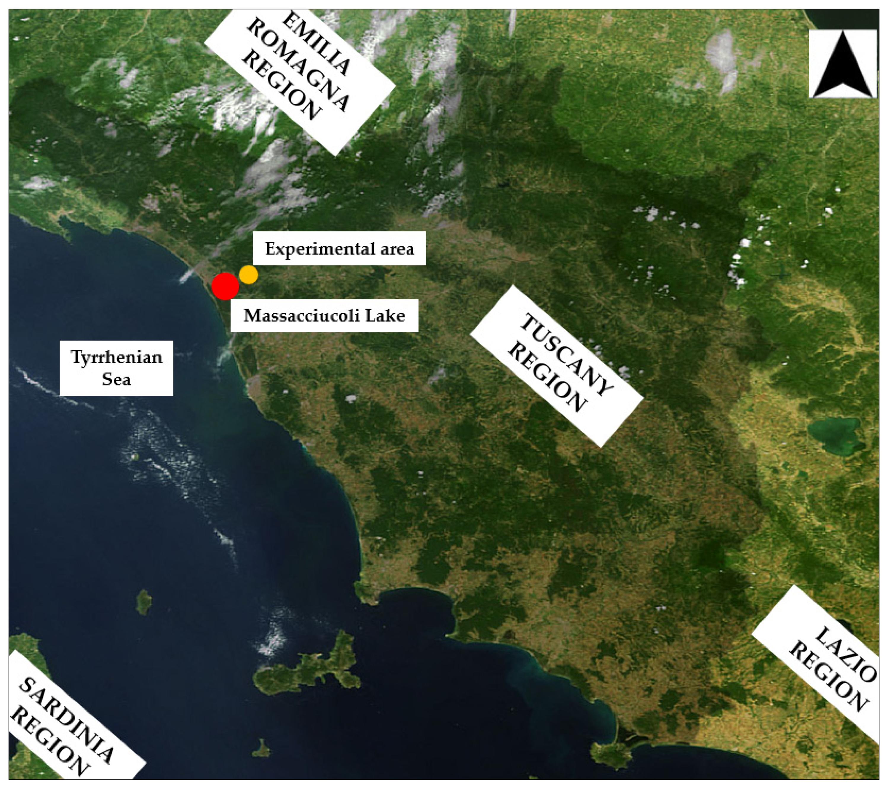
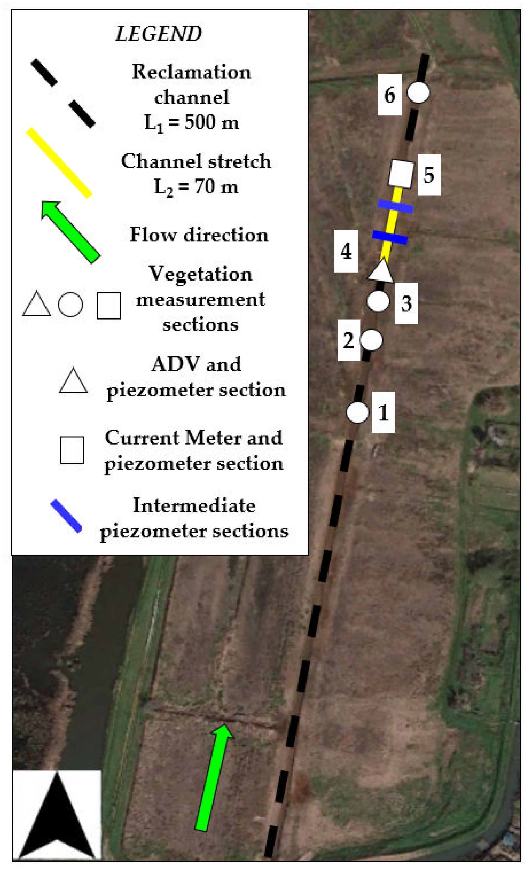
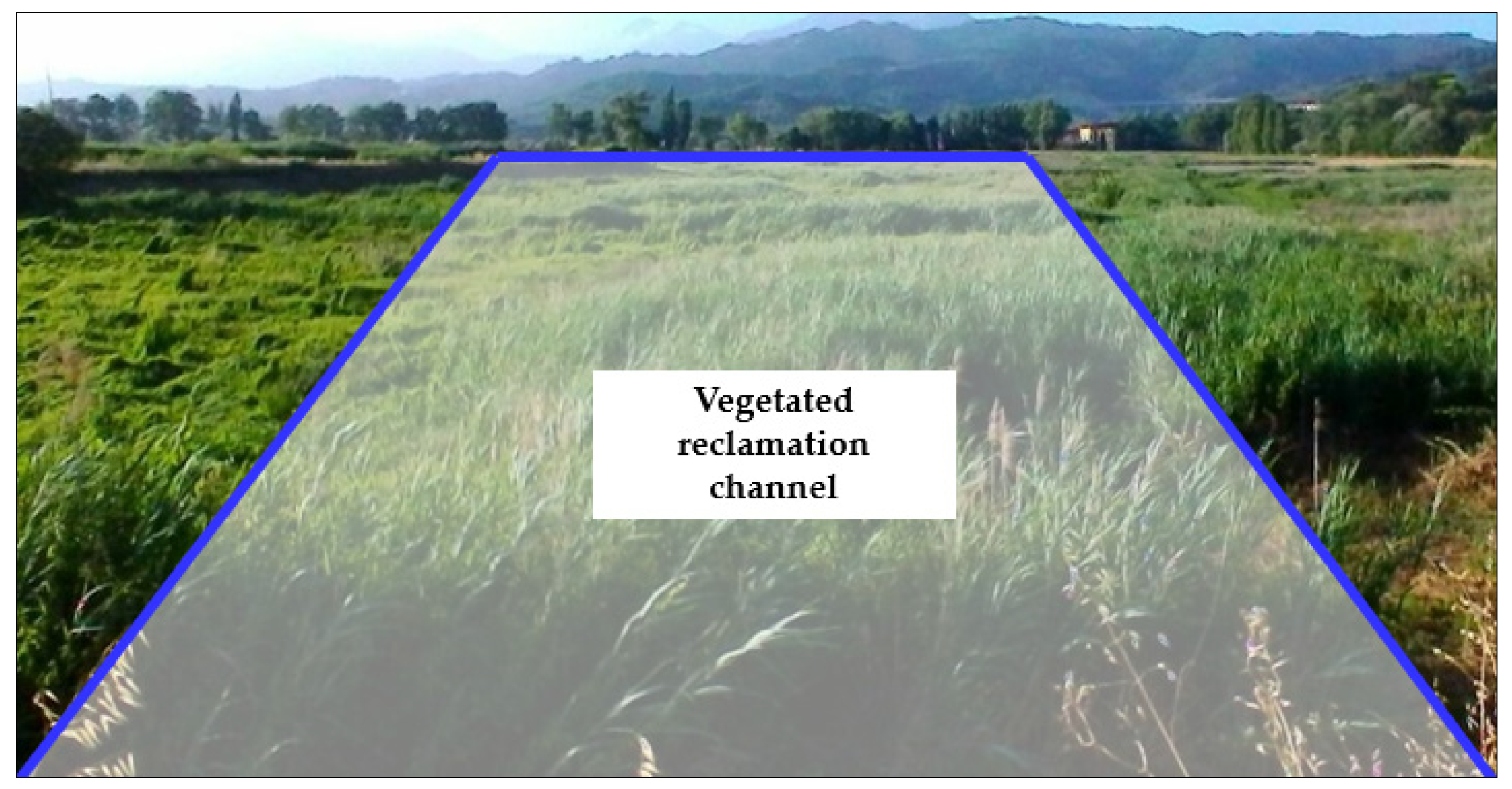
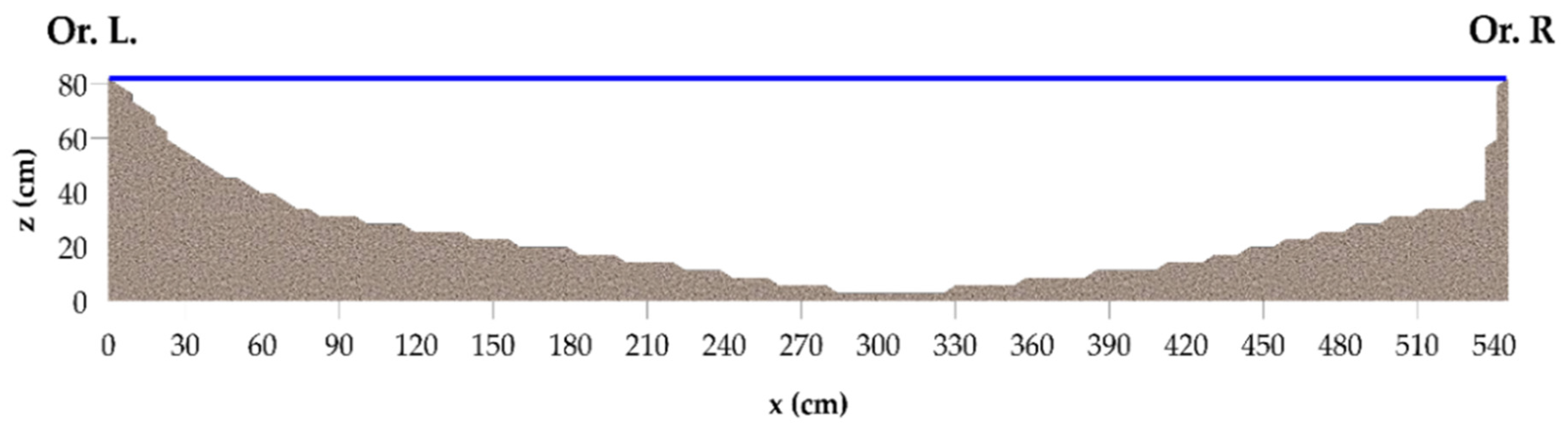
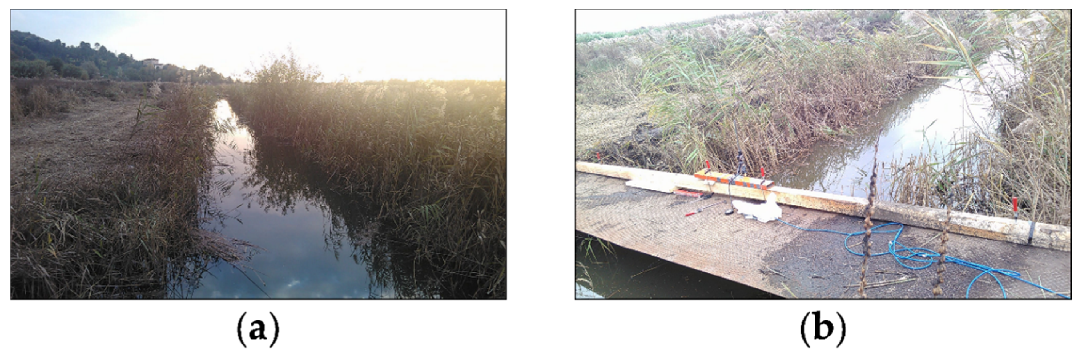
2.1. Experimental Area

The vegetative and hydrodynamic (streamwise velocities and water levels) field measurements were conducted in an abandoned vegetated reclamation channel, which drained field plots that had not been cultivated in the previous 5 years [1,10]. As depicted in Figure 1, the vegetated reclamation channel belongs to a lowland in hydraulic connection with the Massaciuccoli Lake, located in northern Tuscany (Italy).
The 500-m long vegetated reclamation channel was covered by emergent Common reed, at a dormant phenological stage [1]. Field hydrodynamic and vegetation measurements were taken at six cross sections of the vegetated reclamation channel (Figure 2).
The distances between pairs of adjacent cross sections were the following:
-
Cross sections 1–2: 39 m;
-
Cross sections 2–3: 28 m;
-
Cross sections 3–4: 27 m;
-
Cross sections 4–5: 70 m;
-
Cross sections 5–6: 35 m.
The field hydrodynamic and vegetation measurements were designed to characterize the hydraulic properties (cross sectional flow velocity fields and hydraulic gradient), and the reed plant density and morphometrical properties (diameter and height from the channel bottom). As indicated by Errico et al. [1], to reduce the uncertainties during the field hydrodynamic measurements, the hydrodynamic analyses were restricted to a 70-m long experimental stretch of the 500-m long channel, since in this stretch the cross sections were almost uniform in shape. The vegetational measurements were taken along only half of the 500-m long channel because the other half was not easily accessible, because of the presence of gas pipes, hydraulic crossings, and small bridges.

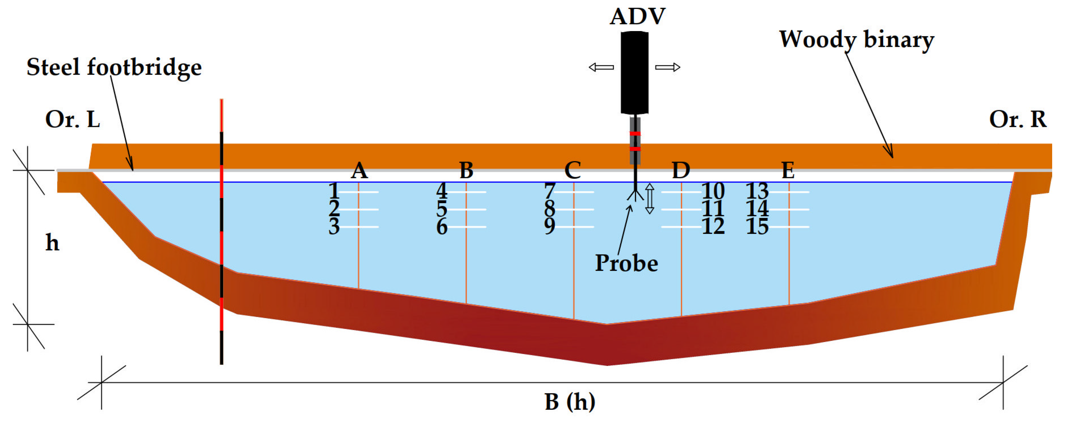
2.2. Field Hydrodynamic Experiments

The field hydrodynamic experiments inside the 70-m long experimental channel stretch were carried out with six different flow rates. In this study, we examine just the two flow rates that were established under the condition of partial riparian vegetation cover. Following Errico et al. [1], hereinafter these two flow rates are respectively referred to as Q2 = 0.16 m3·s−1 and Q3 = 0.33 m3·s−1. The other flow rates not examined in this study are: one with full vegetation coverage, equal to 0.126 m3·s−1; three with no vegetation coverage, respectively equal to 0.086 m3·s−1, 0.175 m3·s−1, and 0.277 m3·s−1.
Because of time constraints and limited available resources for the field campaign, we have not been able to explore a larger number of flow rates and water levels.
The flow rates were established by four mobile hydro-pumps, regulated by the engines of four agricultural tractors: two hydro-pumps were discharging into the entire reclamation channel, at the upstream end, by pumping the water from the adjacent Massaciuccoli Lake; the other two were pumping at the same flow rate out of the channel, at downstream end. The pumping regimes at the beginning and the end of the 500-m long vegetated reclamation channel have been simultaneously regulated to establish stationary conditions during the field hydrodynamic experiments. Stationary flow has been assumed to be verified when the water levels measured at the stages of four cross sections (Section 4, Section 5 and two intermediate cross sections located at a mutual distance of approximately 23 m apart) were verified to be stable for a time interval of 30 min. Flow rate Q2 corresponds to the minimum flow rate achievable with the pumping system deployed in the field, while flow rate Q3 corresponds to the channel flow at bankfull stage.

2.3. Measurements of the Morphometrical Vegetation Properties

Morphometrical properties of the examined riparian vegetation (stem diameters, plant’s heights and density, defined as the number of plants for unit bed surface area) have been measured along the wetted perimeters of the six selected cross sections of the reclamation channel (Figure 3).
Details about the riparian vegetation field survey activity can be found in the study by Errico et al. [1].
The measured field morphometrical vegetation properties have been afterward employed as input parameters of the two resistance predictor models examined in the present study.

2.4. Measurements of the Hydrodynamic Characteristics

The upstream cross section of the experimental reclamation channel stretch (indicated as Section 4 in Figure 2) was selected for the flow velocity measurements (mean flow velocity and turbulence fluctuations [16,17]). A 3-component Nortek® acoustic Doppler velocimeter (ADV) Vectrino II device has been employed, equipped with a 4-beam down-looking probe. The ADV cross section is illustrated in Figure 4.
Many studies dealing with the interaction between water flow and riparian vegetation have been conducted by employing ADV devices, especially in laboratory flumes [17,18], but just in few cases it has been employed in real manmade channels covered by living riparian vegetation [1,5]. An OTT® C31 propeller-type universal current meter has been located at the downstream cross section of the experimental reclamation channel stretch (indicated as Section 5 in Figure 2) to monitor the water flow velocity aiming at verifying the continuity of the water flow volume in the experimental channel stretch [1].
As indicated in Figure 2, the ADV local flow velocity measurements have been taken at 15 points, uniformly distributed along five hydrometric vertical lines spaced 65-cm apart (Figure 5). Three measuring points have been investigated at each hydrometric line, corresponding respectively to depths of 0.05, 0.17, and 0.27 m below the water surface. The ADV measurement depths from the water surface have been maintained fixed, regardless of the water level registered under each examined flow rates in the vegetated reclamation channel.
The ADV raw data are represented by continuous signals over time. Then, in order to improve the quality of the local flow velocity measurements [1], they have been pre-processed [19,20] to remove the noise from the acquired signals. As reported in Errico et al. [1], the values of the signal to noise ratio (SNR, expressed in dB) referred to the two flow rates examined in this study were equal to 38.05 dB and 55.77 dB for Q2 and Q3 flow rates, respectively. Both SNR values are higher than the minimum threshold value reported by Goring and Nikora [20], which is equal to 15 dB.
The hydraulic gradient has been calculated as the slope of the water surface, retrieved from the water level measurements realized at four piezometers distributed along the experimental channel stretch [1,21], as indicated in Figure 2.

2.5. Partial Riparian Vegetation Coverage

The condition of partial riparian vegetation coverage has been obtained by mechanically removing all stems falling inside a 2.70 m wide central region of the entire reclamation channel [1], by means of machinery employed in riparian Common reed management activities [22,23], leaving two side buffers of undisturbed riparian vegetation (Figure 6a). Previous studies have highlighted that with this type of vegetation management strategy it is possible to mitigate the disturbance of the riparian habitat while increasing the channel conveyance to values comparable with that obtained by totally clearing the riparian vegetation [1,5,24]. In the case of partial riparian vegetation coverage, the flow velocity measurements have been conducted by sliding the ADV device along the entire wetted perimeter, in order to characterize the flow fields in correspondence of both the clear and the vegetated regions of the measuring cross section, and, most importantly, at their physical interface, as indicated in Figure 6b.
During the field hydrodynamic experiments, we observed the presence of dead leaves, stems, and rhizomes at the reclamation channel bottom, concentrated in a 10–15 cm thick layer, because of the mechanical action of the cutting machinery. This residual vegetative material importantly affected the cross sectional velocity distributions and, hence, the experimental global flow resistance, as illustrated in the study by Errico et al. [1].

2.6. Measured Vegetative Chézy’s Flow Resistance Coefficients: Cr, meas

Under the assumptions of uniform flow established in the reclamation channel characterized by a condition of partial riparian vegetation coverage, the measured Cr (m1/2·s−1) values, hereinafter referred to as Cr, meas, have been calculated according to the following expression for Q2 and Q3 flow rates, in order to assess the experimental global water flow resistance:
C r ,   m e a s = U R · J ,
where U (m·s−1) is the water flow average velocity, R (m) is the hydraulic radius, and J is the slope of the total energy line. The Cr,meas values computed for the flow rates Q2 and Q3 without considering the DCM in combination with the four composite cross section methods [12,13,14,15] are respectively equal to 4.31 and 8.25 m1/2·s−1.

2.7. Modeled Vegetative Chézy’s Flow Resistance Coefficients: Cr,mod

2.7.1. Bp and S&S Resistance Predictor Models

The two global flow resistance predictor models examined in this study (Bp and S&S [8,9]) have been proposed for real riparian vegetation in emergent condition, i.e., when the water level (h) is smaller than the height of the stems measured from the vegetated reclamation channel bottom (hv). Since the reed stems in the dormant phenological stage are characterized by a rigid biomechanical behavior [25], the two resistance predictor models have to be applied according to the following expressions:
Bp model resistance predictor model [8]:
C r = 1 1 C b 2 + C D · a · h 2 · g ,
where Cb (m1/2·s−1) is the Chézy’s coefficient flow resistance because of the bed roughness in vegetative emergent condition [26], and CD is the stem’s drag coefficient, equal to 1 for rigid cylindrical stems, as in our case. As indicated by Vargas-Luna et al. and Baptist [4,27], Cb can be calculated according to the following expression:
C b = 18 · l o g ( 12 · h k s ) ,
where ks (m1/2·s−1) is the characteristic bed roughness coefficient, equal to 50 m1/2·s−1 for sand.
S&S resistance predictor model [9]:
C r = 1.385 · ( 1 d · m ) · g a · h ,
where d (m) is the average stems’ diameter, m (m−2) is the riparian vegetation density (number of stems per unit channel bed surface), a = m·d (m) is the so-called projected riparian plant area per volume [4,27] and g (m·s−2) is the gravity acceleration.

2.7.2. DCM and Composite Cross Section Methods

In the present study, four composite cross section methods have been employed for characterizing the effect of the non-uniform vegetation distribution along the wetted perimeter on the global flow resistance: Colebatch [12], Horton [13], Pavlovskii [14], and Yen [15]. These methods consider different weights for parametrizing the contribution of the three distinct DCM sub-sections on Cr, according to the following expressions:
Colebatch’s composite cross section method [12]:
C r = ( i = 1 N σ i · C r i 1.5 σ ) 2 3
Horton’s composite cross section method [13]:
C r = ( i = 1 N χ i · C r i 1.5 χ ) 2 3
Pavlovskii’s composite cross section method [14]:
C r = ( i = 1 N χ i · C r i 2 χ ) 1 2
Yen’s composite cross section method [15]:
C r = i = 1 N χ i · C r i R i 1 6 χ R 1 6
where N is the number of the DCM sub-sections, while σi, χi, Ri, and C r i respectively are the flow cross sectional area, the wetted perimeter, the hydraulic radius, and the vegetative Chézy’s flow resistance coefficients calculated employing both Bp and S&S resistance predictor models [8,9] at each of the three DCM sub-sections (excluded DCM sub-section 2 in which the riparian vegetation was absent), while σ, χ, and R are the same parameters referred to the entire ADV cross section. The outcomes of these methods are hereinafter defined as Cr,mod.

2.8. Comparative Analysis between Cr,mod and Cr,meas

The modeled vegetative Chézy’s flow resistance coefficients, indicated as Cr,mod, have been compared with the experimental ones, indicated as Cr,meas, in order to evaluate their capability in predicting the experimental global flow resistance of vegetated channels for a condition of partial reed coverage at real scale.
We first compared Cr, meas with the outcomes of Bp and S&S resistance predictor models [8,9], estimated without considering the actual cross sectional flow velocity distributions, and then, we carried out a second analysis comparing Cr,meas with those obtained by combining Bp and S&S resistance predictor models [8,9] with the four cross section methods [12,13,14,15]. In both cases, the predictive efficiencies of the combination of the two examined resistance predictor models [8,9] have been assessed by computing the relative prediction error (εr, in %), for each of the two examined flow rates: Q2 and Q3, that can be expressed according to the following equation:
ε r ( % ) =   C r , m o d     C r , m e a s C r , m e a s

3. Results

3.1. Measured Vegetative Chézy’s Flow Resistance Coefficients: Cr,meas

3.1.1. Field Morphometrical Vegetation Properties

The quantitative values of the field morphometrical vegetation properties recorded at the six measuring cross sections distributed along the reclamation channel are summarized in Table 1.
In Table 1, num. is the total number of plants for each of the six cross sections and λ = (π·m·d2/4) is the so-called riparian vegetation surface density [4]. It is easy to observe that the cross sectional riparian vegetation distributions, synthetically expressed by λ, resulted to be very similar for all the six examined cross sections and thus it was assumed to be homogeneous along the entire reclamation channel, as already highlighted in Errico et al. [1]. Thus, also both experimental and modeled Cr retrieved at just the ADV cross section have been assumed to be representative of the conditions of the entire partly vegetated reclamation channel.

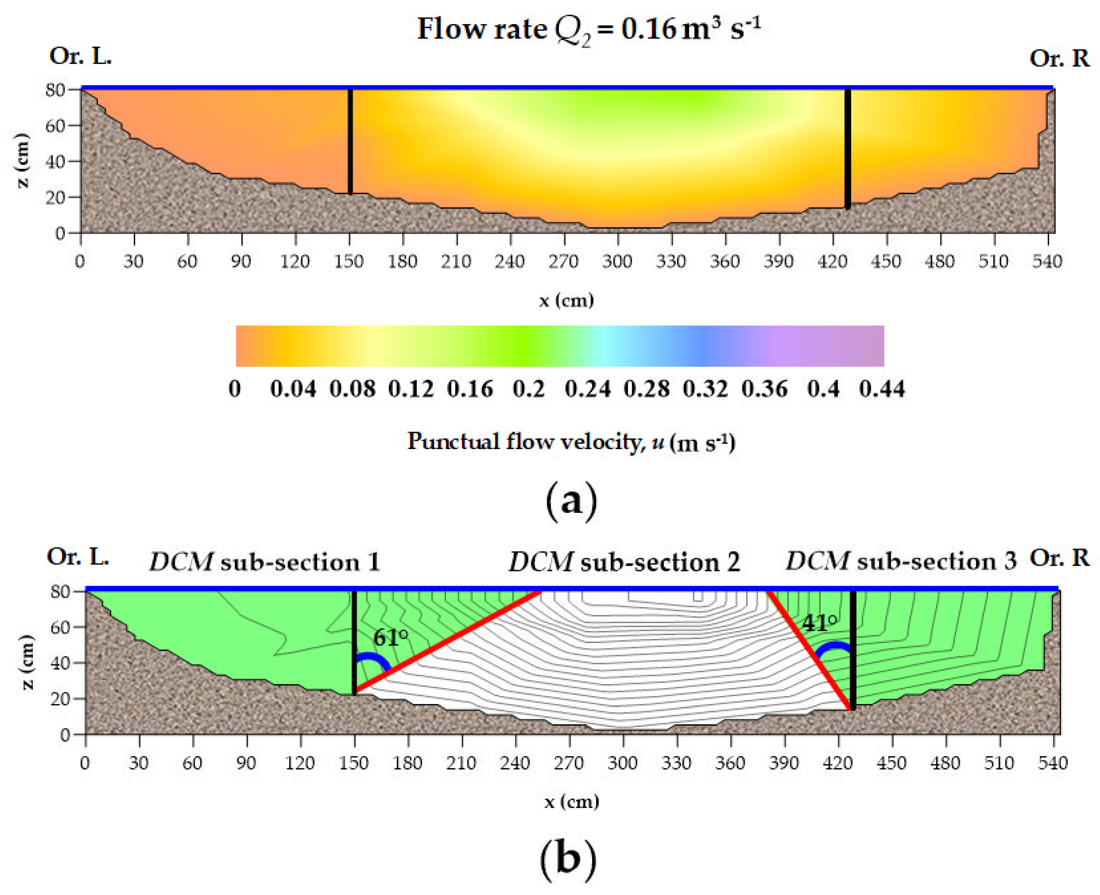
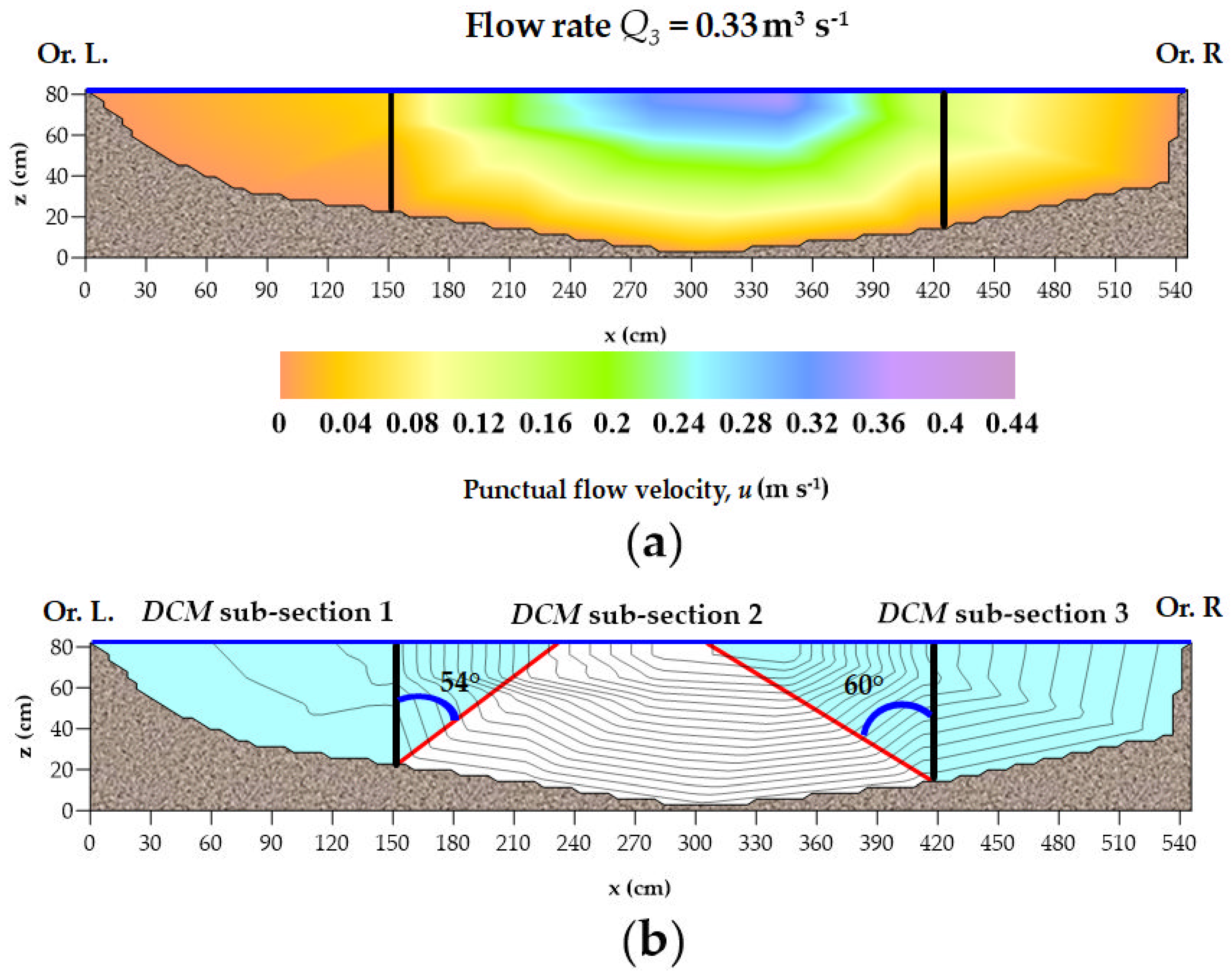
3.1.2. Cross Sectional Velocity Distributions

The experimental flow velocity distributions, also defined as isotachs, have been obtained by linearly interpolating the measured instantaneous flow velocities u (m·s−1) acquired at the 15 points composing the ADV cross section measuring grid [1]. The experimental isotachs corresponding to the two examined flow rates Q2 (= 0.16 m3·s−1) and Q3 (= 0.33 m3·s−1) are respectively shown in Figure 7a and Figure 8a. Three distinct sub-sections have been then defined by applying DCM, after a detailed analysis of the experimental isotachs. As shown in Figure 7b and Figure 8b, the boundaries of the three DCM sub-sections have been delineated by drawing lines orthogonal to the isotachs starting from the channel bottom. Then, the slopes of these lines have been easily determined by means of simple geometrical computations. These lines correspond to the physical interface between water flow and riparian vegetation. The momentum exchange is null through these lines.
The side buffers of undisturbed riparian vegetation notably influenced the cross sectional flow velocity distribution for both Q2 and Q3 flow rate regimes, concentrating the water flow in the central region, cleared from vegetation, as depicted in Figure 7a and Figure 8a. This phenomenon generates strong flow velocity gradients at the physical interface between the riparian vegetation buffers and the water flow [1] (continuous vertical black lines in Figure 7b and Figure 8b) and affects significantly the slope of the boundary lines of the three DCM sub-sections: DCM sub-section 1, DCM sub-section 2 and DCM sub-section 3 (continuous vertical red lines in Figure 7b and Figure 8b).
The Q2 and Q3 flow rate regimes were characterized by a turbulent water flow regime, since the Reynolds numbers Re (= U·h/ν, where U (m·s−1) is the average flow velocity, h (m) is the water level at bankfull, and ν (m2·s−1) is the kinematic viscosity of water, equal to approximately 10−6 m2·s−1) referred to these flow rates were respectively equal to 4.1 × 10⁴ and 8.3 × 10⁴. These values refer to the original values of hydraulic radius R, but they can be considered acceptable also for the condition of partial riparian vegetation cover, since the new values of R, referred to DCM sub-section 2 in which the flow motion was essentially concentrated, are similar to the original ones.

3.1.3. Bp and S&S Combined with Composite Cross Section Methods

The input parameters of the formulas of the four composite cross section methods examined in the present study [12,13,14,15], for each of the three DCM sub-sections described in the previous Section 3.1.2, are summarized in the following Table 2 and Table 3, respectively referred to the two analyzed flow rates: Q2 and Q3. More in detail, χi and σi have been derived by considering separately the three DCM sub-sections delimited by the red borders indicated in Figure 7b and Figure 8b, while hi are the water levels at bankfull, measured from the bottom of each DCM sub-section, and mi are the numbers of recorder stems per unit area, based on the survey plots 1 m × 1 m employed for the vegetation survey [1] falling into each DCM sub-section.
The riparian vegetation density mi at DCM sub-section 2, corresponding to the central region of the entire examined reclamation channel, is null because the Common reed plants have been completely removed in that specific DCM sub-section [1].

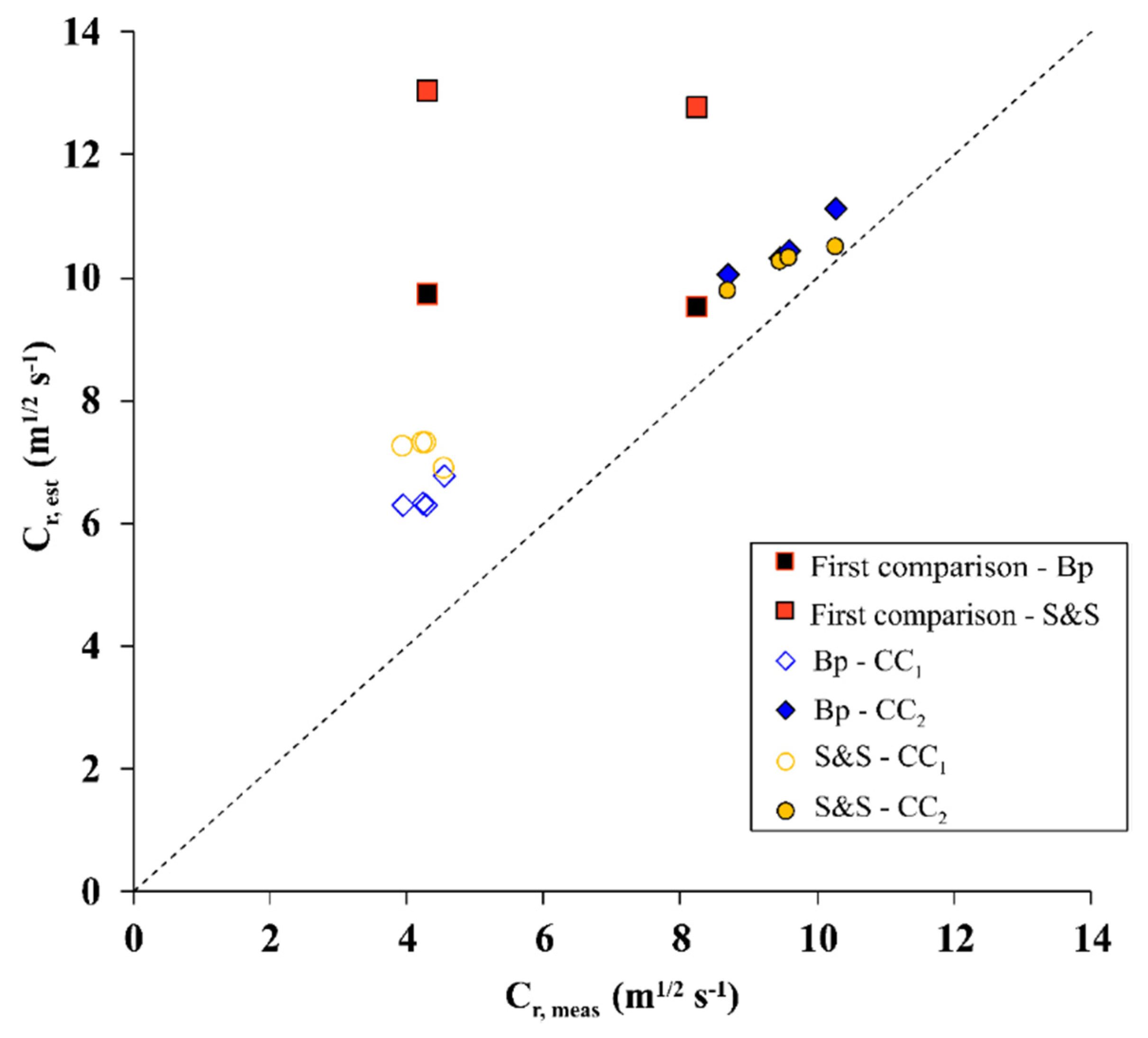
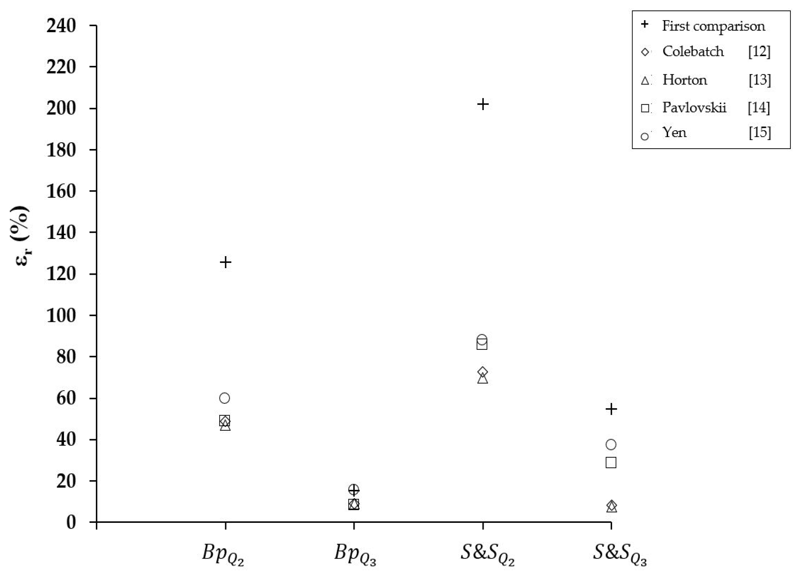
3.1.4. Comparative Analysis between Cr,mod and Cr,meas

A comparative analysis between Cr,mod and Cr,meas has been carried out in order to evaluate the predictive efficiency of the Bp and the S&S flow resistance predictor models [8,9] in the condition of partial vegetation cover of a reclamation channel. As shown in the following Figure 9, a first comparison has been executed between Cr,mod and Cr,meas, the latter calculated without applying the composite section methods (indicated by filled orange and black squares). Then, by employing the methodology proposed in the present study to parametrize the effect of riparian vegetation on the actual cross sectional flow velocity distribution, a comparative analysis has been performed by applying the DCM [11] in combination with the four selected composite cross section methods: Colebatch [12], Horton [13], Pavlovskii [14], and Yen [15].
Both Bp and S&S resistance predictor models [8,9] overestimated the measured Cr. The only remarkable difference between the two selected resistance predictor models is represented by the changing trend of the modeled Cr, depending on the two different investigated flow rates, as it can be noticed in Figure 9. In fact, for the Q2 flow rate, Bp resistance predictor model [8] returned higher values than S&S [9], while this behavior was inverted when considering the Q3 flow rate.
The relative prediction error εr (%) between Cr, mod and Cr,meas for the two examined resistance predictor models [8,9], for the Q2 and Q3 flow rates are shown in Figure 10. The combination of the two resistance predictor models examined in the present study [8,9] with the four composite cross section methods [12,13,14,15] for the two examined flow rates are respectively labeled as Bp Q 2 , Bp Q 3 , S & S Q 2 , and S & S Q 3 .
It can be easily observed that the Yen composite cross section method [15] systematically returned the highest εr value, for both Bp and S&S resistance predictor models [8,9] under both Q2 and Q3 flow rates. On the other hand, we can observe that in three cases Horton method [13] always returned the lower εr values, except for the case of S&S resistance predictor model [9] in combination with Pavlovskii method [14] under the Q3 flow rate regime. In just one specific case, corresponding to Bp resistance predictor model [8] under the Q3 flow rate regime, Yen composite cross section methods [15] returned εr = 16%, close to that obtained by applying Bp and S&S resistance predictor models [8,9] without combining them with the four composite cross section methods, equal to 15%. For the Q2 flow rate, εr reduced from 126% to 47% by combining Bp model [8] with Horton composite cross section method [13], and from 202% to 70% for S&S resistance predictor model [9] combined with the same method, while, for the Q3 flow rate, εr decreased from 15% to 8% for Bp model [8] combined with Pavlovskii composite cross section method [14] and from 55% to 7% for S&S resistance predictor model [9] in combination with Horton composite cross section method [13]. Moreover, as it can be easily noticed, the highest reduction of εr with respect to the first comparison has been obtained by combining Bp resistance predictor model [8] with Horton composite cross section method [13], for the Q2 flow rate.

4. Discussion

It is possible to notice from the analysis of the outcomes of the proposed methodology that the S&S resistance predictor model [9], in combination with Horton composite cross section method [13] exhibited the highest predictive performance, testified by the lowest εr, equal to 7%, achieved for the Q3 flow rate. The Horton composite cross section method [13] assumes that the flow velocity is the same in the three DCM sub-sections; this assumption is not rigorously reliable for our study case, where it has been observed that DCM sub-section 2 carried most of the flow (Figure 7a and Figure 8b). However, it led to reasonable results in terms of hydraulic roughness, comparable with those retrieved by employing the Colebatch method [14], because the wetted perimeters χi and the flow cross sectional area σi of each DCM sub-section are very similar, being the channel width of an order of magnitude lager than the water levels at bankfull.
Our results are in agreement with Yang et al. [28], who achieved a minimum prediction error (indicated in their work as relative accuracy) equal to 9.14%, computed by comparing the global flow resistances based on field measurements with those retrieved by employing a model based on unmanned aerial vehicles (UAV) techniques, in a river partially covered by emergent riparian vegetation. This is a promising finding since it demonstrates that the application of a simple methodology, like DCM [11] combined with one of the four examined composite cross section methods [12,13,14,15], can lead to results comparable with those obtained by using more complex models. The satisfactory levels of accuracy reached by the methodology proposed in the present study, testified by small εr values, have been achieved owing to the detailed analysis of the experimental ADV cross sectional flow velocity fields, that significantly affect the contributions of the different regions of the reclamation channel cross section to the global flow resistance for a condition of partial vegetation cover.
Moreover, the variability range of the εr values is very similar to that reported by Errico [29], which compared modeled and experimental roughness coefficients by applying different predictive models [30,31,32] in combination with the same composite cross section methods tested in the present study [12,13,14,15], but for a different scenario of partial vegetation coverage in a reclamation channel colonized by green and flexible Common reed plants. The main difference with respect to our outcomes is represented by the choice of the borders of the DCM sub-sections. In fact, Errico [29] considered just the vertical flow-vegetation physical interfaces, instead of those derived from the analysis of the experimental isotachs.
The evidences of the comparative analysis based on the proposed methodology can provide quantitative suggestions to administrators of land reclamation areas about the most appropriate methods for the parametrization of the field morphometrical vegetation properties that mostly affect the global flow resistance at real scale in partly vegetated reclamation channels [1,5], as a direct consequence of the hydrodynamic interaction between water flow and rigid Common reed plants in emergent conditions. In fact, the proposed methodology leads to a significant improvement in the accuracy of the examined resistance prediction models, with respect to those obtained without applying it. The presented findings are referred to the specific case of reclamation channels colonized by Common reed distributed along two lateral buffers at the sides. This aspect may constitute a limitation for the application on other riparian environments. However, we believe that in most vegetated channels the cross-sectional partitioning can represent a significant improvement of the global flow resistance estimation.
Further applications of the proposed methodology will be carried out on datasets obtained by remote sensing techniques from UAV, largely employed for measuring field morphometrical and bio-mechanical properties of vegetation in many agricultural, forestry, as well as in ecohydraulic studies referred to different vegetation species and phenological stages [29,33,34].

5. Conclusions

A direct comparative analysis between modeled and measured vegetative Chézy’s coefficients Cr has been carried out, for assessing the predictive efficiencies of the Bp and the S&S resistance predictor models [8,9] for an experimental reclamation channel partly vegetated by rigid and emergent riparian Common reed plants, under two different flow rates. The accuracy of both resistance predictor models has been sensibly improved with respect to those obtained without applying the composite cross section methods [12,13,14,15]. These results have been achieved by applying a more rigorous physically based methodology, that considers the actual influence of the cross sectional riparian vegetation distribution on the flow velocity fields in conditions of partial reed cover. The proposed methodology, preliminarily introduced by Lama et al. [3], is founded on the analysis of the experimental isotachs retrieved from local ADV measurements at the upstream channel cross section [1]. We combined the Bp and S&S resistance predictor models [8,9] with DCM [12] and with four composite cross section methods: Colebatch [12], Horton [13], Pavlovskii [14], and Yen [15]. From the outcomes of the direct comparison between modelled and measured vegetative Chézy’s coefficients Cr, it was observed that combination of the S&S resistance predictor model [8] and the Horton composite cross section method [13] returned the lowest value of relative prediction error εr, equal to 7%. The results of this study are limited to channels having a width of an order of magnitude lager than the water levels at bankfull.
From a computational fluid dynamics (CFD) perspective, the DCM constitutes a very simple model, based on basic theoretical assumptions. At the same time, it represents a quick method for describing the contribution of the distinct portions of the entire cross section characterized by the condition of partial riparian vegetation coverage. A significant improvement in the accuracy of the outcomes of the present study can be obtained by means of 2D and 3D numerical simulations, aiming at reproducing the actual impacts of the full and partial riparian vegetation coverage on the water flow velocity and turbulence cross sectional fields, by modelling the Common reed stems as rigid cylindrical elements. Another improvement to this methodology can be achieved by analyzing the flow velocity vertical profile in detail, especially in correspondence of the interface between riparian vegetation buffers and water flow. In these cases, we can also consider the other methods (i.e., Kouwen et al. [35]) aiming at defining the influence of vegetation patches on global flow resistance.
It is possible to conclude that the outcomes of this study can provide to administrators of reclamation areas a simple and accurate methodology for modeling the real-scale effects of the cross sectional streamwise distributions on the global flow resistance of artificial and natural partly vegetated water bodies.

Notation

aprojected riparian plant area per volume
ADVacoustic Doppler velocimeter
Bwidth of the ADV cross section
BpBaptist et al. (2007) resistance predictor model
B p Q 2 Baptist et al. (2007) resistance predictor model results for flow rate Q2
B p Q 3 Baptist et al. (2007) resistance predictor model results for flow rate Q3
CbChézy’s coefficient flow resistance due to the bed roughness
CDstem’s drag coefficient
CFDcomputational fluid dynamics
Crvegetative Chézy’s flow resistance coefficient
Cr, measmeasured vegetative Chézy’s flow resistance coefficient
Cr, meodmodeled vegetative Chézy’s flow resistance coefficient
daverage stems’ diameter
DCMdivided channel method
f”vegetative Darcy-Weisbach’s friction factor
ggravity acceleration
hwater level at bankfull of the entire ADV cross section
hiwater level at bankfull of each DCM sub-section
hvplants’ height from the bottom of the vegetated reclamation channel
kscharacteristic bed roughness coefficient, equal to 50 m1/2 s−1 for sand
mvegetation density of the entire ADV cross section
mivegetation density of each DCM sub-section
Nnumber of the DCM sub-sections
nManning’s hydraulic roughness coefficient
num.number of stems recorded in each measuring cross section
Q2first examined flow rate, equal to 0.16 m3 s−1
Q3second examined flow rate, equal to 0.33 m3 s−1
Rhydraulic radius of the entire ADV cross section
Rihydraulic radius of each DCM sub-section
ReReynolds number
S&SStone and Shen (2002) resistance predictor model
S & S Q 2 Stone and Shen (2002) resistance predictor model results for flow rate Q2
S & S Q 3 Stone and Shen (2002) resistance predictor model results for flow rate Q3
Uaverage flow velocity
uinstantaneous flow velocity
ε r relative prediction error
λriparian vegetation surface density
νkinematic viscosity of water, equal to approximately 10−6 m2 s−1
πpi, equal to approximately 3.14
σflow cross sectional area of the entire ADV cross section
σiflow cross sectional area of each DCM sub-section
χwetted perimeter of the entire ADV cross section
χiwetted perimeter of each DCM sub-section

Author Contributions

Conceptualization and methodology, G.F.C.L. and A.E.; validation, S.F., L.S., F.P. and G.B.C.; investigation, G.F.C.L., A.E. and S.F.; writing—original draft preparation, G.F.C.L.; writing—review and editing, A.E., S.F., L.S., F.P. and G.B.C.; funding acquisition, F.P. All authors read and approved the final manuscript.

Funding

This research was funded by Interreg EU project “Assistere l’adattamento ai cambiamenti climatici dei sistemi urbani dello spazio transfrontaliero—ADAPT, Interreg Italia-Francia Marittimo 2014-2020 CUP B19J1600289000”.

Acknowledgments

The authors want to kindly thank Consorzio di Bonifica 1 Toscana Nord for funding the research, Eng. Leonardo Giannecchini and his staff for their help during the field experiments. Special thanks go to Eng. Daniele Maffi for the field vegetative and hydrodynamic measurements, including the ADV raw data pre-processing. The authors also acknowledge the four anonymous reviewers for their constructive comments which helped in improving the paper.

Conflicts of Interest

The authors declare no conflict of interest.

References

  1. Errico, A.; Lama, G.F.C.; Francalanci, S.; Chirico, G.B.; Solari, L.; Preti, F. Flow dynamics and turbulence patterns in a reclamation channel colonized by Phragmites australis (common reed) under different scenarios of vegetation management. Ecol. Eng. 2019, 133, 39–52. [Google Scholar] [CrossRef]
  2. Rowinski, P.M.; Västilä, K.; Aberle, J.; Järvelä, J.; Kalinovska, M.B. How vegetation can aid in coping with river management challenges: A brief review. Ecohydrol. Hydrobiol. 2018, 8, 345–354. [Google Scholar] [CrossRef] [Green Version]
  3. Lama, G.F.C.; Errico, A.; Francalanci, S.; Chirico, G.B.; Solari, L.; Preti, F. Comparative analysis of modeled and measured vegetative Chézy’s flow resistance coefficients in a reclamation channel vegetated by dormant riparian reed. In Proceedings of the International IEEE Workshop on Metrology for Agriculture and Forestry, Portici, Italy, 24–26 October 2019. [Google Scholar]
  4. Vargas-Luna, A.; Crosato, A.; Uijttewaal, W.S.J. Effects of vegetation on flow and sediment transport: Comparative analyses and validation of predicting model. Earth Surf. Proc. Land. 2015, 40, 157–176. [Google Scholar] [CrossRef]
  5. Errico, A.; Pasquino, V.; Maxwald, M.; Chirico, G.B.; Solari, L.; Preti, F. The effect of flexible vegetation on flow in reclamation channels. Estimation of roughness coefficients at real scale. Ecol. Eng. 2018, 120, 411–421. [Google Scholar] [CrossRef]
  6. Västilä, K.; Järvelä, J. Modeling the flow resistance of woody vegetation using physically based properties of the foliage and stem. Water Resour. Res. 2014, 50, 229–245. [Google Scholar] [CrossRef]
  7. Caroppi, G.; Västilä, K.; Järvelä, J.; Rowinski, P.M.; Giugni, M. Turbulence at water-vegetation interface in open channel flow: Experiments with natural-like plants. Adv. Water Resour. 2019, 127, 180–191. [Google Scholar] [CrossRef]
  8. Baptist, M.J.; Babovic, V.; Rodríguez, J.; Keijzer, M.; Uittenbogaard, R.; Mynett, A.; Verwey, A. On inducing equations for vegetation resistance. J. Hydraul. Res. 2007, 45, 435–450. [Google Scholar] [CrossRef]
  9. Stone, B.M.; Shen, H.T. Hydraulic resistance of flow in channels with cylindrical roughness. J. Hydraul. Eng. 2002, 128, 500–506. [Google Scholar] [CrossRef]
  10. Errico, A.; Lama, G.F.C.; Francalanci, S.; Chirico, G.B.; Solari, L.; Preti, F. Validation of global flow resistance models in two experimental reclamation channels covered by Phragmites australis (common reed). In Proceedings of the 38th IAHR World Congress, Panama City, Panama, 1–6 September 2019. [Google Scholar]
  11. Chow, V.T. Open Channel Hydraulics; McGraw-Hill: New York, NY, USA, 1959. [Google Scholar]
  12. Colebatch, G.T. Model tests on the Lawrence Canal roughness coefficients. J. Inst. Civil Eng. (Australia) 1941, 13, 27–32. [Google Scholar]
  13. Horton, R.E. Separate roughness coefficients for channel bottoms and sides. Eng. News-Rec. 1933, 111, 652–653. [Google Scholar]
  14. Pavlovskii, N.N. On a design formula for uniform flow in channels with nonhomogeneous walls. Trans. All-Union Sci. Res. Inst. Hydraulic Eng. 1931, 3, 157–164. (In German) [Google Scholar]
  15. Yen, B.C. Open channel flow resistance. J. Hydraul. Eng. 2002, 128, 20–39. [Google Scholar] [CrossRef]
  16. Scotto di Perta, E.; Agizza, M.A.; Sorrentino, G.; Boccia, L.; Pindozzi, S. Study of aerodynamic performance of different wind tunnel configurations and air inlet velocities, using computational fluid dynamics (CFD). Comput. Electron. Agr. 2016, 125, 137–148. [Google Scholar] [CrossRef]
  17. Caroppi, G.; Gualtieri, P.; Fontana, N.; Giugni, M. Vegetated channel flows: Turbulence anisotropy at flow–rigid canopy interface. Geosciences 2018, 8, 259. [Google Scholar] [CrossRef] [Green Version]
  18. Ozan, A.Y.; Yilmazer, D. Near-Wake Flow Structure of a Suspended Cylindrical Canopy Patch. Water 2019, 12, 84. [Google Scholar] [CrossRef] [Green Version]
  19. Goring, D.G.; Nikora, V.I. Despiking Acoustic Doppler Velocimeter Data. J. Hydraul. Eng. 2002, 128, 117–126. [Google Scholar] [CrossRef] [Green Version]
  20. King, A.T.; Tinoco, R.O.; Cowen, E.A. A k–ε turbulence model based on the scales of vertical shear and stem wakes valid for emergent and submerged vegetated. J. Fluid Mech. 2012, 701, 1–39. [Google Scholar] [CrossRef]
  21. Lama, G.F.C.; Errico, A.; Francalanci, S.; Chirico, G.B.; Solari, L.; Preti, F. Hydraulic modeling of field experiments in a reclamation channel under different riparian vegetation scenarios. In Proceedings of the AIIA Mid-Term Conference, Matera, Italy, 12–13 September 2019. [Google Scholar]
  22. Rhee, D.S.; Woo, H.; Kwon, B.; Ahn, H.K. Hydraulic resistance of some selected vegetation in open channel flows. River Res. Appl. 2008, 24, 673–687. [Google Scholar] [CrossRef]
  23. Faugno, S.; Quaquarelli, I.; Civitarese, V.; Crimaldi, M.; Sannino, M.; Ricciaridello, G.; Caracciolo, G.; Asirelli, A. Two-steps Arundo Donax L. harvesting in South Italy. Chem. Eng. Trans. 2017, 58, 265–270. [Google Scholar]
  24. Soana, E.; Bartoli, M.; Milardi, M.; Fano, E.A.; Castaldelli, G. An ounce of prevention is worth a pound of cure: Managing macrophytes for nitrate mitigation in irrigated agricultural watersheds. Sci. Total Environ. 2019, 647, 301–312. [Google Scholar] [CrossRef]
  25. Pasquino, V.; Saulino, L.; Pelosi, A.; Allevato, E.; Rita, A.; Todaro, L.; Saracino, A.; Chirico, G.B. Hydrodynamic behaviour of European black poplar (Populus nigra L.) under coppice management along Mediterranean river ecosystem. River Res. Appl. 2018, 34, 1–9. [Google Scholar] [CrossRef]
  26. van Velzen, E.; Jesse, P.; Cornelissen, P.; Coops, H. Stroming-Sweerstand Vegetatie in Uiterwaarden; Handboek. Part 1 and 2; Technical Report, RIZA Reports: Arnhem, The Netherland, 2003. [Google Scholar]
  27. Baptist, M.J. Modelling floodplain biogeomorphology. Ph.D. Thesis, Delft University of Technology, Delft, The Netherlands, 2005. [Google Scholar]
  28. Yang, S.; Wang, P.; Lou, H.; Wang, J.; Zhao, C.; Gong, T. Estimating River Discharges in Ungauged Catchments Using the Slope–Area Method and Unmanned Aerial Vehicle. Water 2019, 11, 2361. [Google Scholar] [CrossRef] [Green Version]
  29. Errico, A. The effect of flexible vegetation on flow in drainage channels. Field surveys and modelling for roughness coefficients estimation. Ph.D. Thesis, University of Florence, Florence, Italy, 2017. [Google Scholar]
  30. Nepf, H.M.; Vivoni, E.R. Flow structure in depth-limited, vegetated flow. J. Geophys. Res. 2000, 105, 28457–28557. [Google Scholar] [CrossRef]
  31. James, C.S.; Birkhead, A.L.; Jordanova, A.A.; O’Sullivan, J.J. Flow resistance of emergent vegetation. J. Hydraul. Res. 2004, 42, 390–398. [Google Scholar] [CrossRef]
  32. Yang, W.; Choi, S.-U. A two-layer approach for depth-limited open-channel flows with submerged vegetation. J. Hydraul. Res. 2010, 48, 466–475. [Google Scholar] [CrossRef]
  33. Sarghini, F.; De Vivo, A. Analysis of Preliminary Design Requirements of a Heavy Lift Multirotor Drone for Agricultural Use. Chem. Eng. Trans. 2017, 58, 635c620. [Google Scholar]
  34. Giannetti, F.; Chirici, G.; Gobakken, T.; Næsset, E.; Travaglini, D.; Puliti, S. A new approach with DTM-independent metrics for forest growing stock prediction using UAV photogrammetric data. Remote Sens. Environ. 2018, 213, 195–205. [Google Scholar] [CrossRef]
  35. Kouwen, N.; Unny, T.E.; Hill, H.M. Flow retardance in vegetated channels. J. Irrig. Drain. Div. 1969, 95, 329–342. [Google Scholar]
Figure 1. Location of the experimental area (indicated by the yellow filled circle), in hydraulic connection with the adjacent Massacciucoli Lake (indicated by the red filled circle). (From https://www.esa.int/ESA_Multimedia/Images/2010/07/La_Toscana_vista_da_Envisat, modified).
Geosciences 10 00047 g001
Figure 2. Surveyed cross sections (1–6) along the 500-m long vegetated reclamation channel, indicated by the black dashed line. The 70-m long experimental channel stretch is indicated by the yellow continuous line. The white filled circles indicate the measuring sections employed for the measurements of the vegetative morphometrical properties, while the white filled triangle and square represent the ADV and current meter measuring cross section, which coincides with the upstream cross section of the 70 m long experimental channel stretch, also employed for the water tables measurements. The blue continues lines indicate the other two intermediate water level measuring cross sections. (From Lama et al. [3], modified).
Geosciences 10 00047 g002
Figure 3. View of the 500-m long vegetated reclamation channel. The continuous blue lines indicate the borders of the vegetated reclamation channel.
Geosciences 10 00047 g003
Figure 4. Acoustic Doppler velocimeter (ADV) cross section. The continuous dark blue line indicates the water level at bankfull.
Geosciences 10 00047 g004
Figure 5. Scheme of the ADV measuring points (1–15), uniformly distributed along five hydrometric lines (A–E). The ADV moved along a woody binary installed on a steel footbridge, and then blocked at each measuring point during the acquisitions. The two parameters h (m) and B (m) are respectively the water level and width at bankfull of the ADV cross section, which vary according to the flow rate. The continuous dark blue line indicates the water level at bankfull. (from Errico et al. [1], modified).
Geosciences 10 00047 g005
Figure 6. (a) Examined vegetated reclamation channel in condition of partial riparian vegetation coverage; (b) local ADV flow velocity measurement set-up, for the two investigated flow rate regimes Q2 = 0.16 m3·s−1 and Q3 = 0.33 m3·s−1.
Geosciences 10 00047 g006
Figure 7. (a) Flow velocity field u (m·s−1) for the Q2 (= 0.16 m3·s−1) flow rate regime; (b) divided channel method (DCM) sub-sections. The continuous dark blue line indicates the water level at bankfull. The continuous vertical black lines indicate the boundary of the side buffers of undisturbed riparian vegetation, while the red lines represent the borders of the DCM sub-sections, in which slopes were equal to 61° and 41°, respectively referred to DCM sub-section 1 and DCM sub-section 3 (light green regions in Figure 7b). (From Lama et al. [3], modified).
Geosciences 10 00047 g007
Figure 8. (a) Flow velocity field u (m·s−1) for the Q3 (= 0.33 m3·s−1) flow rate regime; (b) DCM sub-sections. The continuous dark blue line indicates the water level at bankfull. The continuous vertical black lines indicate the boundary of the side buffers of undisturbed riparian vegetation, while the red lines represent the borders of the DCM sub-sections, in which slopes were equal to 54° and 60°, respectively referred to DCM sub-section 1 and DCM sub-section 3 (light blue regions in Figure 8b).
Geosciences 10 00047 g008
Figure 9. Measured and modeled Cr (m1/2·s−1) for the Bp and S&S resistance predictors [8,9], by not applying (black and orange filled squares) and applying the four composite cross section methods: the blue diamonds and the yellow circles correspond respectively to Bp and S&S resistance predictor models, for Q2 = 0.16 m3·s−1 (unfilled symbols) and Q3 = 0.33 m3·s−1 (filled symbols). The dashed black line represents the perfect agreement between modeled and measured Cr.
Geosciences 10 00047 g009
Figure 10. Relative prediction errors εr (%) of Bp and S&S resistance predictor models [8,9], computed under the two flow rate regimes respectively pair to Q2 = 0.16 m3·s−1 and Q3 = 0.33 m3·s−1, corresponding to the condition of partial riparian vegetation coverage of the reclamation channel, without employing the proposed methodology (black crosses), and by applying the four examined composite cross section methods: Colebatch [12] (diamonds), Horton [13] (triangles), Pavlovskii [14] (squares), and Yen [15] (circles).
Geosciences 10 00047 g010
Table 1. Morphometrical vegetation properties measured at the six cross sections: num. is the number of stems in each measuring cross section, d (m) is the average stems’ diameter, m (m−2) is the riparian vegetation density and λ =(π·m·d2/4) is the riparian vegetation surface density.
Cross Sectionnum.d (m)m (m−2)λhv (m)
12700.0054640.001462.50
21650.0065390.001302.30
31590.0065380.001262.23
41980.0062470.001422.10
51820.0069430.001612.35
62450.0055580.001382.50
Table 2. Hydraulic and vegetative parameters referred to the flow rate Q2 = 0.16 m3·s−1: χi (m), σi (m2), hi (m) and mi (m−2) are respectively the wetted perimeter, the flow cross sectional area, the water level at bankfull and the riparian vegetation density of each DCM sub-section.
DCM Sub-Sectionχi (m)σi (m−2)hi (m)mi (m−2)
11.710.970.6849
22.771.460.71-
31.520.800.6578
Table 3. Hydraulic and vegetative parameters referred to the flow rate Q3 = 0.33 m3·s−1: χi (m), σi (m2), hi (m) and mi (m−2) are respectively the wetted perimeter, the flow cross sectional area, the water level at bankfull and the riparian vegetation density of each DCM sub-section.
DCM Sub-Sectionχi (m)σi (m−2)hi (m)mi (m−2)
11.881.040.7249
22.821.210.77-
31.820.960.6878

