Soil–Structure Interaction Assessment of the 23 November 1980 Irpinia-Basilicata Earthquake


1
School of Engineering and Built Environment, Griffith University, Engineering Building (G09), Engineering Drive, Southport 4222, Australia
2
Department of Civil and Environmental Engineering, Te Whare Wānanga o Tāmaki Makaurau-University of Auckland, 20 Symonds Street, Auckland 1010, New Zealand
*
Author to whom correspondence should be addressed.
Geosciences 2020, 10(4), 152; https://0-doi-org.brum.beds.ac.uk/10.3390/geosciences10040152
Submission received: 17 March 2020
/
Revised: 20 April 2020
/
Accepted: 20 April 2020
/
Published: 22 April 2020
(This article belongs to the Special Issue The November 23rd, 1980 Irpinia-Lucania, Southern Italy Earthquake: Insights and Reviews 40 Years Later)
Abstract
:This paper aimed to present a systematic study of the effects caused by the strong earthquake that struck southern Italy on 23 November 1980 (Ms = 6.9) and affected the Campania and Basilicata regions. Two aspects are discussed here: The broadening of the knowledge of the response site effects by considering several soil free-field conditions and the assessment of the role of the soil–structure interaction (SSI) on a representative benchmark structure. This research study, based on the state-of-the-art knowledge, may be applied to assess future seismic events and to propose new original code provisions. The numerical simulations were herein performed with the advanced platform OpenSees, which can consider non-linear models for both the structure and the soil. The results show the importance of considering the SSI in the seismic assessment of soil amplifications and its consequences on the structural performance.
1. Background
The 23 November 1980 Irpinia–Basilicata (Southern Italy) earthquake (Ms = 6.9) caused deep changes in the urban socio-economic layout, and primary and secondary effects that brought about changes to the natural environment, such as landslides (e.g., Senerchia, Buoninventre, Caposele, Calitri, San Giorgio La Molara, and Grassano) [1,2,3,4]. It consisted of several rupture episodes, which occurred at 0.18 and 40 s from the foreshock, and it was assigned a surface-wave magnitude of Ms = 6.9 [5,6]. A wide area (about 3500 km2) recorded serious damage, many casualties, and 15 localities were almost destroyed, including Sant’Angelo dei Lombardi, Laviano, Lione, Santomenna, Senerchia, Pescopagano, and Balvano. It was estimated that of a total of approximately 1.85 million buildings involved in the event, 75,000 were destroyed, 275,000 seriously damaged, and 480,000 slightly damaged [6].
With respect to this event, the documentary sources are based on two main typologies of technical data preserved in local archives: The “Scheda A” and “Scheda B”, which report the damages to the buildings, consisting mostly of reinforced concrete (RC) structures characterized by infill masonry walls (IMWs), which are representative of the Italian residential buildings. Eight damage levels were defined by considering the action to be undertaken, such as repairing works, evacuation, or demolition [6]. Other important documents are the recovery plans (named “Piani di Recupero”) of the historical centers, the other sources used to analyze the outcomes of the earthquake at the urban scale. An important study regarding the effects of spectral accelerations was proposed by [7], who analyzed the effects of the soil on the accelerations in several locations, with particular attention to the Naples area. In addition, [8] simulated the recorded strong-motion data by computing spectral accelerations and peak amplitude residual distributions in order to investigate the influence of site effects and compute synthetic ground motions around the fault. They simulated the expected ground motions varying the hypocenters, the rupture velocities, and the slip distributions and compared the median ground motions and related standard deviations from all scenario events with empirical ground-motion prediction equations (GMPEs). Recent earthquakes, such as the Athens (Greece, 1999) [9], the Kocaeli (Turkey, 1999) [10], the Haiti (2010) [11], and the Gorkha (Nepal, 2015) [12,13,14] earthquakes, showed the importance of taking into account soil amplifications. In the literature, several approaches have been applied to perform ground motion analyses including site effects: hybrid analyses that consist of a combination of probabilistic and deterministic methods (e.g., [15,16]), convolution approaches that provide modifications of the rocking hazard (e.g., [17,18]), and 1D seismic site response analyses (e.g., [19,20]).
Even if the 1980 Irpinia–Basilicata (southern Italy) earthquake is well documented with several contributions (e.g., [21,22,23,24]) and models proposed [25,26], the assessment of the role of the soil on the structural damage is still a relatively unexplored issue and this paper aimed to fill this gap. In particular, the principal aim was to propose numerical simulations of different soil conditions and assess the effects of the soil–structure interaction (SSI), which can significantly affect the seismic vulnerability of structures [27,28,29]. In this regard, when the superficial deposits overlie the bedrock, amplifications of the surface seismic accelerations may not be conservatively predicted by the codes. The so-called site effects consist of a combination of soil and topographical effects, which can modify (amplify and attenuate) the characteristics (amplitude, frequency content, and duration) of the incoming wave field and are primarily based on the geotechnical properties of the subsurface materials [30]. In particular, the response of the superficial layers is strongly influenced by the uncertainty associated to the definition of the soil properties and model parameters that are fundamental to assess the well-known mechanism of seismic amplifications of ground motion [31]. Therefore, accounting for the amplification effects of superficial layers has become critically important in seismic design [32] and widely adopted in many codes’ prescriptions, such as Eurocode 8 [33], ASCE (American Association of Civil Engineering) standards 7-05 [34], and 4-98 [35]. These codes provide soil parameters, generally determined through geological investigations [36,37,38,39,40], that can largely vary even within the same area [41,42]. The methodology followed in this paper consists of a first step, where free-field (FF) analyses were computed on several layers of soil, and secondly, an SSI (Soil-Structure Interaction) analysis was performed on a selected structural configuration that is representative of the buildings that were damaged during the Irpinia-Basilicata earthquake.
2. Case Study
SSI analyses require the definition of geomechanical parameters that are fundamental to describe the dynamic soil behavior, such as the modulus reduction and damping curves (see [43,44]). According to the current state of knowledge on the Irpinia-Basilicata earthquake, strength parameters for superficial layers are not available. Therefore, it was necessary to select representative values based on available information, such as [8], for a preliminary study. These values are herein determined with free-field analyses since the actual values at each building site will slightly differ when the building characteristics are considered. In particular, the present paper aimed to model a low-rise building based on a relatively shallow foundation assuming that the ground motion amplitude, which decreases at the foundation level with respect to the free field, may be negligible [42].
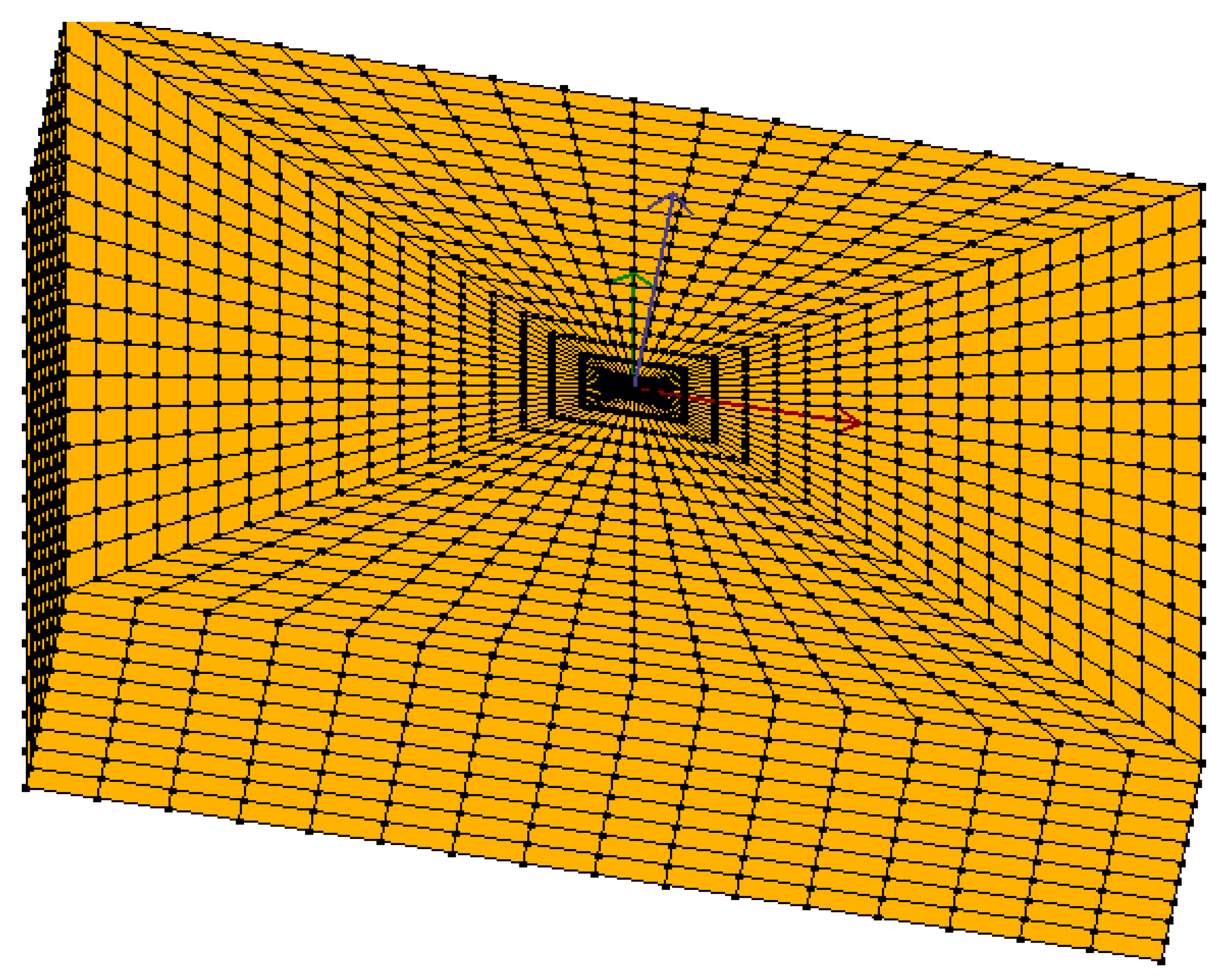
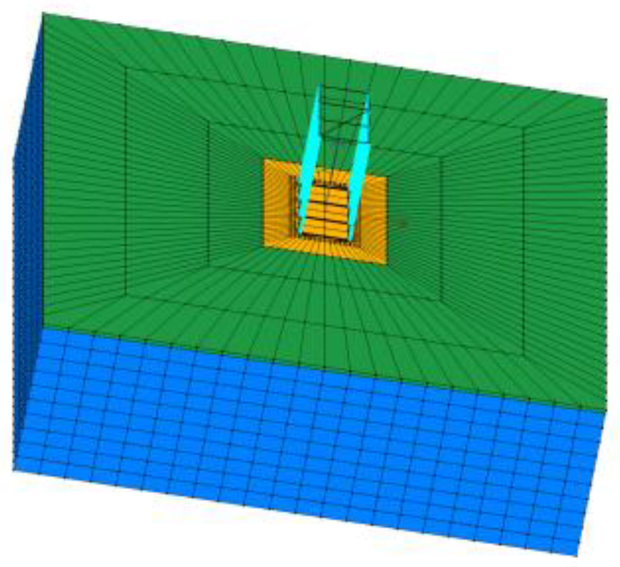
The study here proposed was divided into two steps. First of all, several FF models with different soil conditions were considered (Figure 1), in order to study the effects of soil deformability on the amplification of the motion. In particular, four incoherent soils were performed on the basis of the contributions that were found in the literature. Then, a complete 3D numerical model with the soil-foundation-structure system was performed (Figure 2). The FF soil models consist of a one-layer 20-m-deep homogenous incoherent material with a 3D mesh (Figure 1). The penalty method was adopted for the boundary conditions (tolerance of 10−4), chosen as a compromise for the soil domain definition, which was modelled large enough to ensure strong constraint conditions but not too large in order to avoid problems associated with the equations system conditions. Base boundaries (depth of 20 m) were considered as rigid. Base and lateral boundaries vertical direction (described by the third degree of freedom (DOF)) were constrained, while longitudinal and transversal directions were left unconstrained on the lateral boundaries, in order to allow shear deformations of the soil. The definition of the mesh elements dimension follows the approach already adopted [45,46,47,48] and, in order to verify proper simulation of FF conditions, accelerations at the top of the mesh were compared with the FF ones, which were found to be identical, confirming the effective performance of the mesh. The benchmark structure was calibrated in order to be representative of the buildings that were present in Irpinia in 1980. In this regard, a 3-storey concrete building with masonry walls was considered.
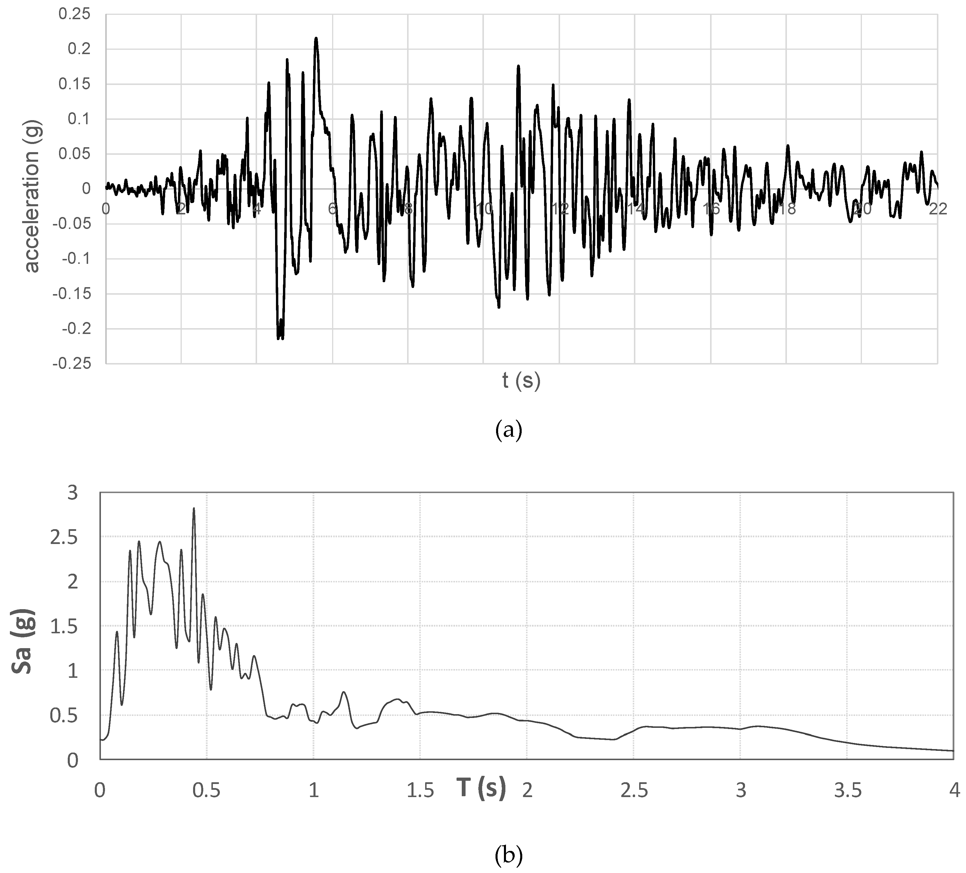
Dynamic analyses were performed with OpenSeesPL. The selected input motion was chosen from the Italian Accelerometric Archive [49] and it represents the acceleration registered in Sturno (STN) station (lat: 41.0183°, long: 15.1117°) in Avellino, Campania (Figure 3), and located less than 5 km from the fault and 33 km from the epicenter (41.76°N, 15.31°E). For more details, see [8]. The input was defined on soil B, as classified by Eurocode 8, and applied at the base of the model along the longitudinal direction.
2.1. Step 1: FF Analyses
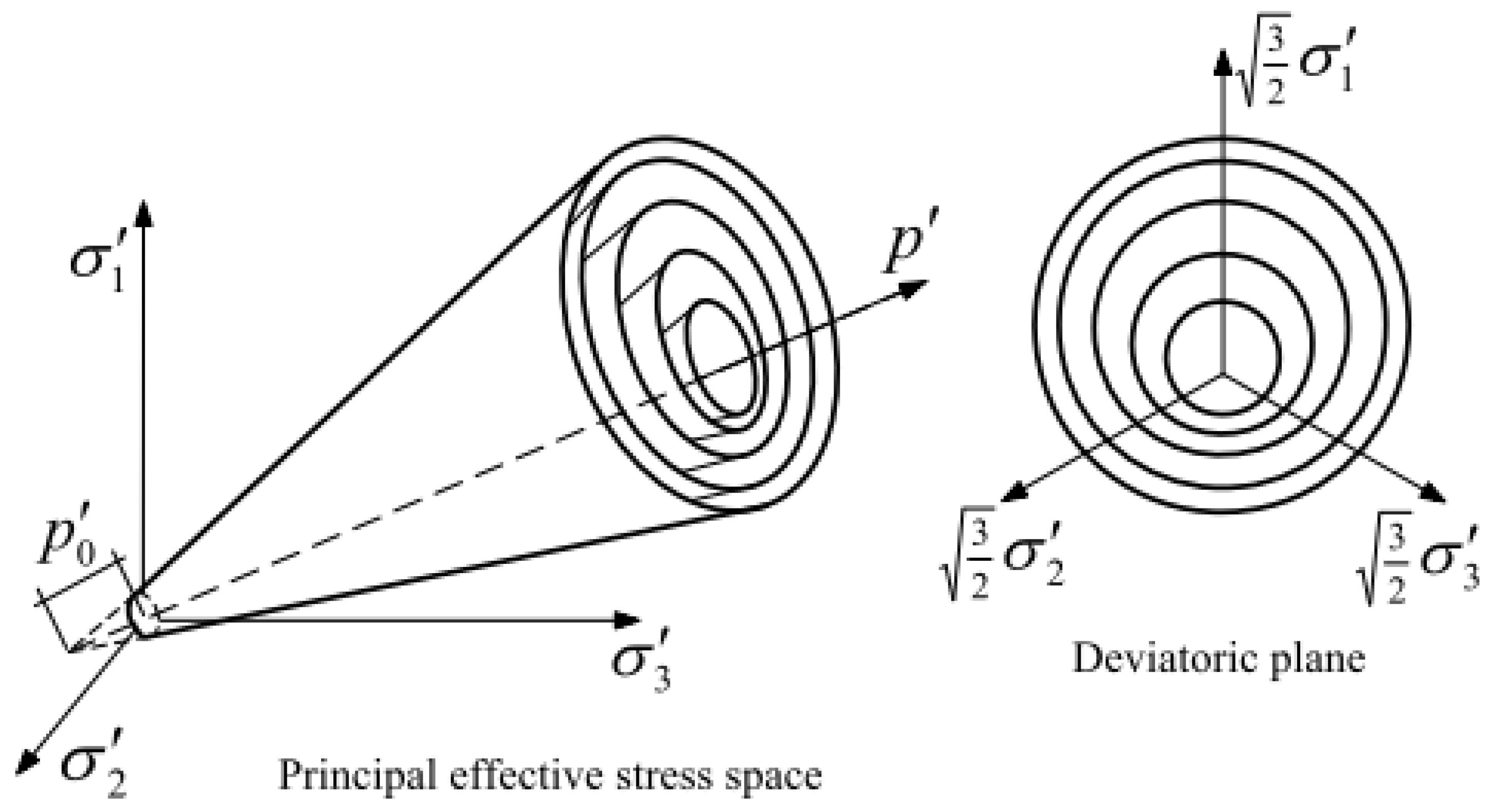
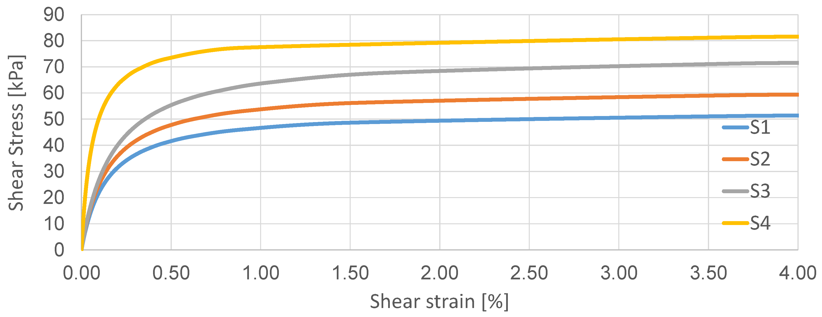
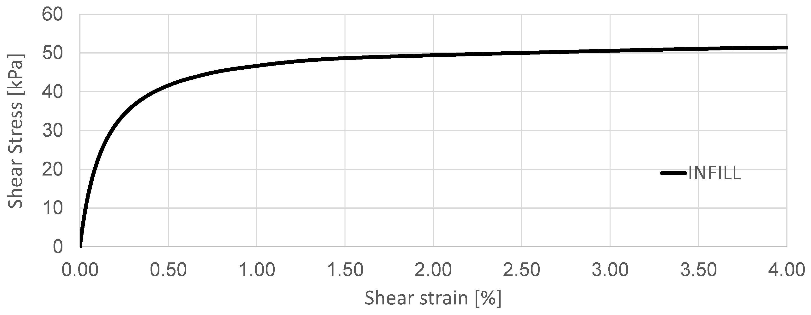
The soil models were built up on a two-phase material following the u-p formulation [50], where u is the displacement of the soil skeleton and p is the pore pressure. The soil material was based on the following assumptions: (1) Small deformations and rotations, as well as solid and fluid densities remain constant in both time and space; (2) porosity is locally homogeneous and constant with time; (3) soil grains are incompressible; and (4) solid and fluid phases are accelerated equally [51]. The 20-m-deep soil layer was defined by the PressureDependMultiYield02 model [52,53], based on the multi-yield-surface plasticity framework developed by [54], in order to reproduce the mechanism of cycle-by-cycle permanent shear strain accumulation in clean sands (Figure 4). Table 1 shows the adopted parameters, such as the low-strain shear modulus and friction angle, as well as the shear wave velocities and permeability. Soil fundamental periods were estimated considering an equivalent uniform linear layer, following [55]. The number of yield surfaces was equal to 20 for all soil models. Figure 5 shows the backbone curves for all the selected soil models.
The 3D soil models consist of a 100 m × 100 m × 20 m mesh, built up with 8000 20-node BrickUP elements and 9163 nodes to simulate the dynamic response of solid-fluid fully coupled material [52,53]. For each BrickUP element, 20 nodes describe the solid translational degrees of freedom, while the eight nodes on the corners represent the fluid pressure 4 degrees of freedom. For each node, Degree of Freedom (DOF)s 1, 2, and 3 represent solid displacement (u) and DOF 4 describes fluid pressure (p), which were recorded using OpenSees Node Recorder [52,53] at the corresponding integration points. The element dimension increases from the structure (center of the model) to the lateral boundaries, which were modelled to behave in pure shear and located far away from the center of the mesh.
2.2. Step 2: SSI Analyses
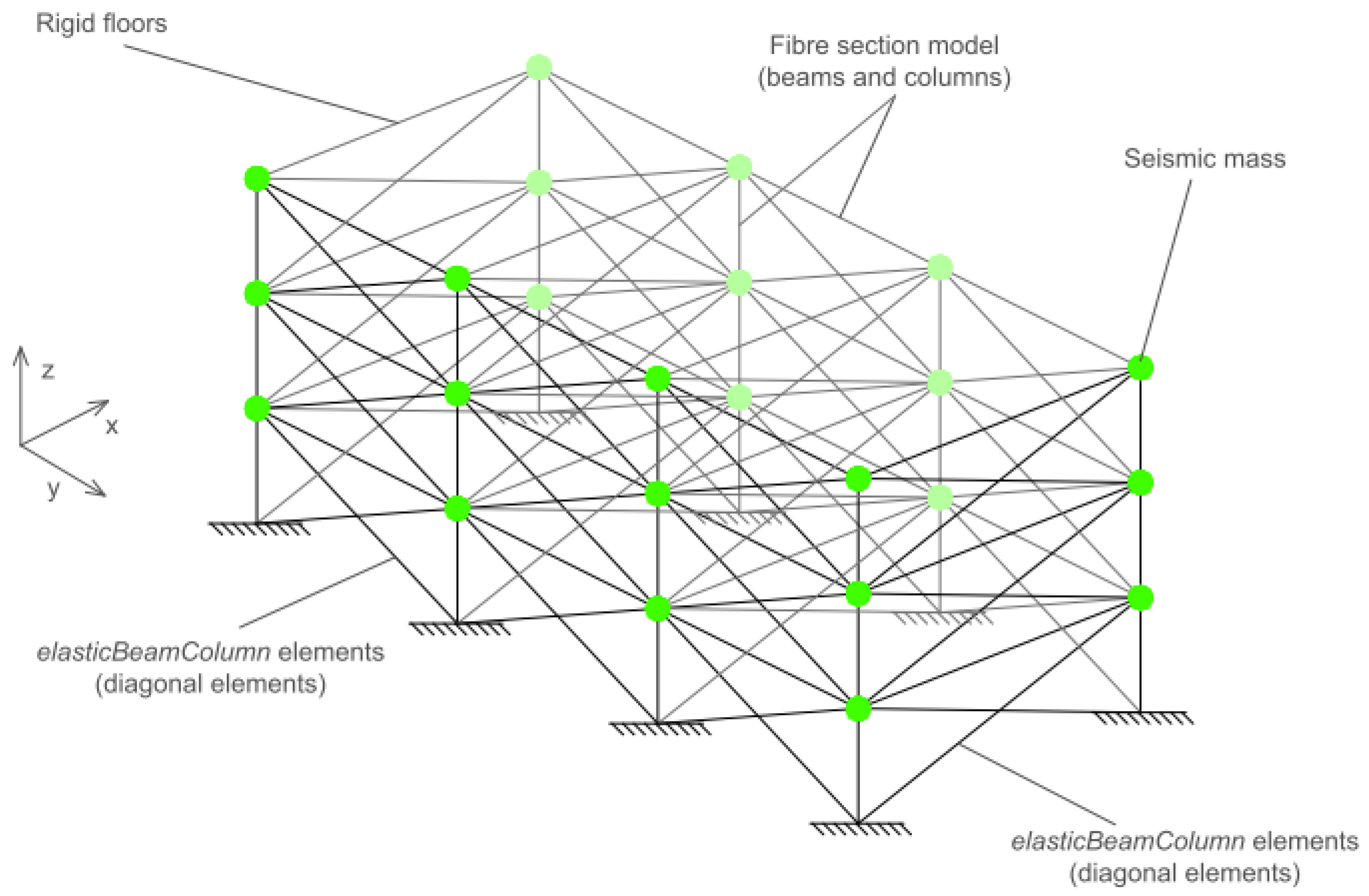
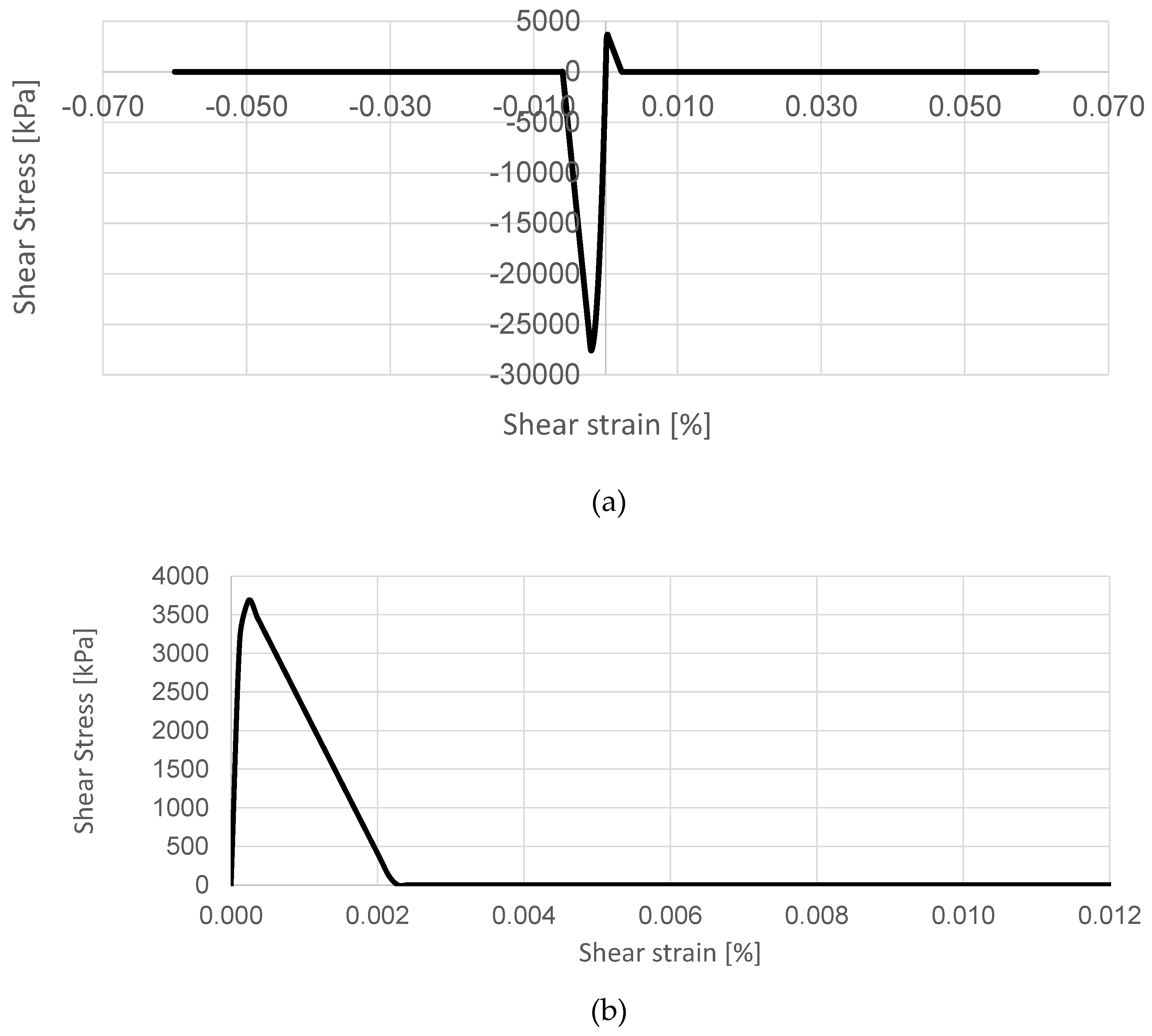
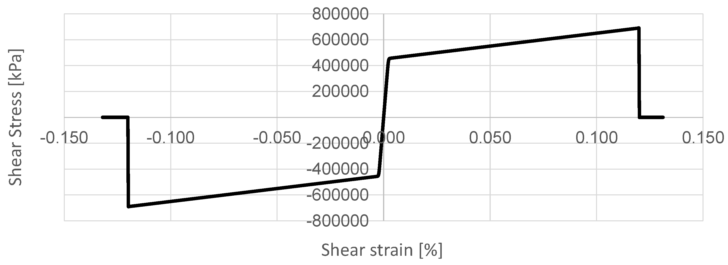
The study considered an RC structure with infill masonry walls as a benchmark, in order to represent the Italian residential buildings that were mostly damaged during the 1980 Irpinia–Basilicata earthquake. The benchmark structure was built with a 4 × 2 column scheme (4 columns in the transversal direction (8 m spaced) and 2 in the longitudinal direction (10 m spaced)) and modelled to have periods in the range of those of residential buildings, considering 3 floors (a 3.4 m storey height, with a total structure height of 10.2 m). The structure was modelled as a superposition of two schemes (Figure 6). Both vertical and horizontal elements were composed by RC concrete columns and beams, respectively, and characterized by fiber section models. Concrete02 material [56,57] was chosen to model the core and the cover portions (Figure 7a,b, respectively) of the section (0.40 m × 0.40 m) and with the parameters defined in Table 2. The ratio between the unloading slope (related to the maximum strength) and the initial slope was taken as equal to 0.1. A total of 30 bars were used and represented by Steel02 material [58], with the properties shown in Table 3 and the ratio between the post-yield tangent and initial elastic tangent equal to 0.01 (Figure 8). The parameters that control the transition from elastic to plastic branches were assumed R0 = 15, CR1 = 0.925 and CR2 = 0.15, as suggested by [53]. The masonry walls were modelled as equivalent diagonal elasticBeamColumn elements [52,53], in both the longitudinal and transversal directions. The masonry walls’ properties were selected based on the Italian code provisions, with low-to-medium mechanical characteristics (Table C8A.2.1 [59]), as shown in Table 4. Table 5 shows the vibration periods of the structure with and without the infill masonry walls. It is worth noting that the masonry walls affect the structural natural period (from 0.3012 s to 0.2085 s), since they increase the lateral stiffness of the whole structure (as shown in [60]). In particular, the infill masonry walls introduce different mechanisms that may significantly modify the seismic behavior of the structure. The foundation was modelled as a 0.50-m-deep rectangular concrete raft foundation (28.4 m × 34.4 m) in order to represent the recurring shallow foundation typologies for residential buildings. These types of foundation can be particularly vulnerable due to their bearing capacity, which depends only on the contact pressure and not on the frictional mechanisms (as in the case of deep foundations). The considered foundation was assumed to be rigid, by tying all the columns base nodes together with those of the soil domain surface, using equalDOF [52,53]. Horizontal rigid beam-column links were set normal to the column longitudinal axis to simulate the interface between the column and the foundation. The foundation was designed by calculating the eccentricity (the ratio between the overturning bending moment at the foundation level and the vertical forces) in the most detrimental condition of the minimum vertical loads (gravity and seismic loads) and maximum bending moments. The foundation was modelled with an equivalent concrete material, by applying the Pressure Independent Multi-Yield model [52,53] (Table 6). This model consists of a non-linear hysteretic material with a Von Mises multi-surface kinematic plasticity model, which can simulate a monotonic or cyclic response of materials whose shear behavior is insensitive to the confinement change. The nonlinear shear stress-strain backbone curve is represented by the hyperbolic relation, defined by the two material constants (low-strain shear modulus and ultimate shear strength) [52,53].
The 3D soil models consist of a 118.4 m × 124.4 m (20.5 m thick) mesh, built up with 31,860 nodes and 35,868 20-node BrickUP elements to simulate the dynamic response of solid-fluid fully coupled material [52,53] and with the same assumptions considered for the free-field models (Section 2.1). As explained in Section 3.1, S2 was implemented amongst the soil materials that were considered in step 1. The first 0.5-m-deep soil layer around the foundation was modelled with a backfill defined by the PressureDependMultiYield [52,53] model, based on the multi-yield-surface plasticity framework developed by [54]. Table 7 shows the adopted parameters, such as the low-strain shear modulus, the friction angle, and the permeability. The number of yield surfaces was equal to 20. Figure 9 shows the backbone curves.
3. Results
In this section, the results are discussed on the basis of the assumptions made so far. In particular, it is important to state that the findings are limited to the conditions considered herein, especially to those regarding the selected soils.
3.1. FF Analyses
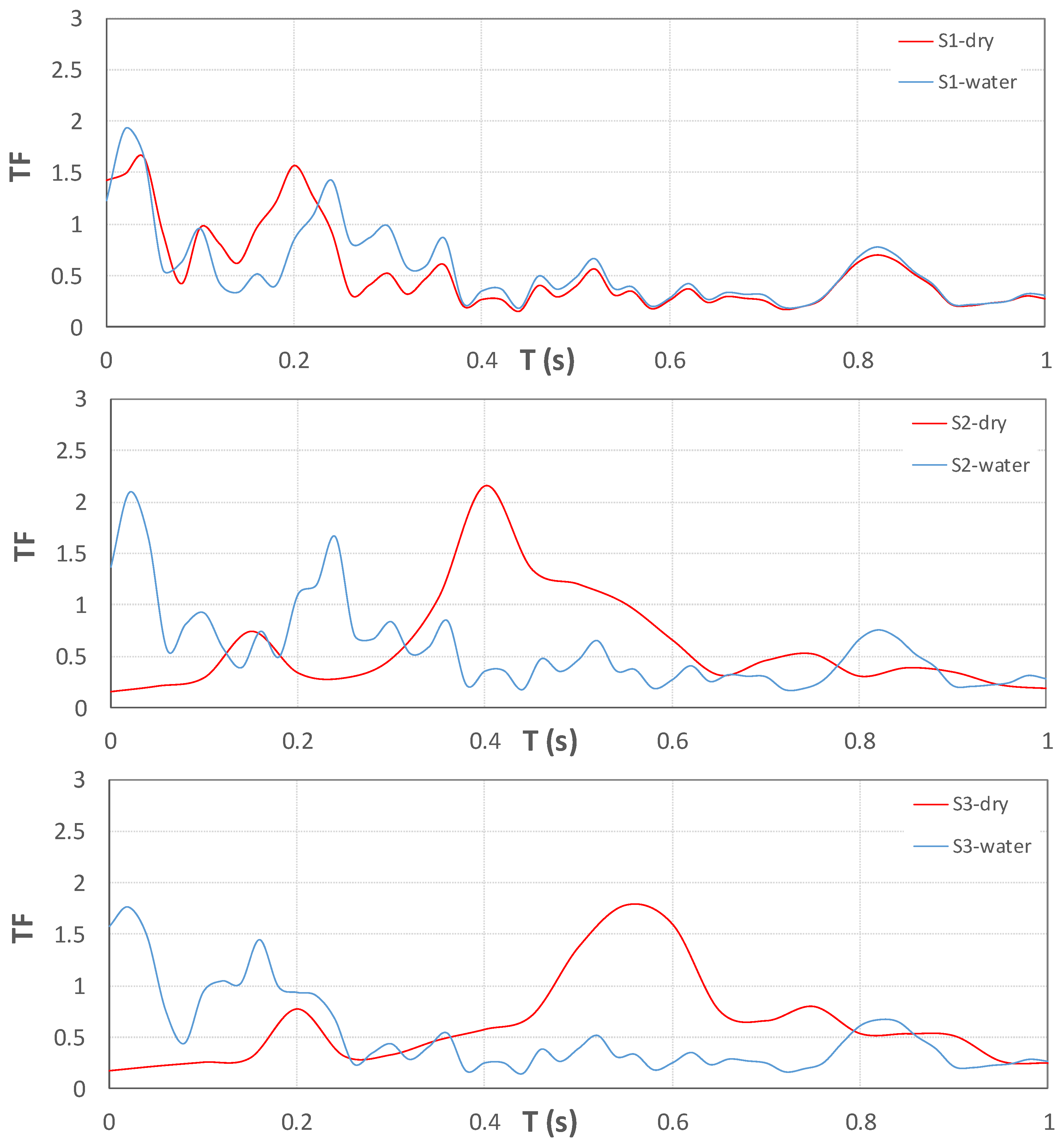
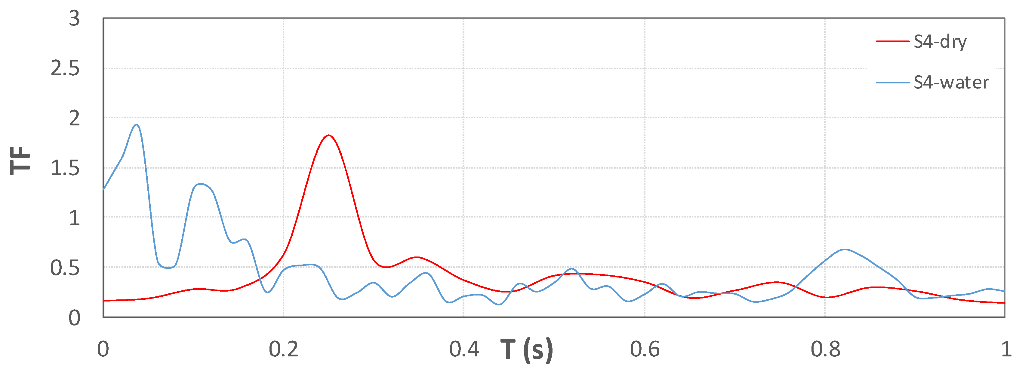
The selected soil profiles were considered under the assumption that the superficial layers are characterized by sand deposits with shear wave velocities in the range of 150–250 m/s. In this regard, the four materials were selected to be representative of real soil conditions from low to medium-low stiffness. Saturated and dry conditions were chosen in order to perform dynamic analyses. The position of the water table is fundamental in order to assess the performance of the system (soil + structure). However, it is extremely difficult to know this parameter in real situations. In this study, the water table depth was set at a depth of 2 m from the ground surface for the saturated condition and for all soil models. For each soil condition, transfer functions (TFs) were calculated as the ratio between the acceleration at the ground surface (depth of 0 m) and the one at the base of the soil domain (depth of 20 m), considering the selected input motion (Figure 3) along the longitudinal axis.
Figure 10 compares the behavior of S1, S2, S3, and S4 for both saturated and dry conditions for the range of periods between 0 and 1 s. It is worth considering that the role of soil deformability in the mechanism of amplification inside the range of periods of the selected structure is paramount (Table 5). In particular, S2 with the saturated condition is shown to be the most detrimental soil above which the structure can be founded (maximum amplification equal to 1.66), since the TF peak occurs in conjunction with the fundamental period of the structure (Table 5), and thus S2 is applied in the SSI model (see Section 3.2). Moreover, dry conditions are noticeable for those periods that are far from the structural ones. In general, it is possible to state that S2, S3, and S4 with the saturated condition are the most detrimental cases. On the other hand, S1 seems to behave differently from the other cases, since dry conditions are more detrimental for the structural configurations that were herein considered.
3.2. SSI Analyses
With the recent development of the performance-based earthquake engineering (PBEE) methodology [61,62,63], there has been an increasing attention in the new engineering demand parameter (EDP) to assess the structural performance of buildings, such as the floor accelerations. In particular, many codes [64,65,66,67] are implementing new provisions based on floor performance. In this regard, the paper aimed to move in the direction of this new approach by calculating not only the peak values of the aforementioned EDP but also the top floor accelerations. This section presents the structural performance at the foundation level and along the height of the building, considering the soil S2 under saturated conditions, which was found to be the most detrimental (Section 3.1).
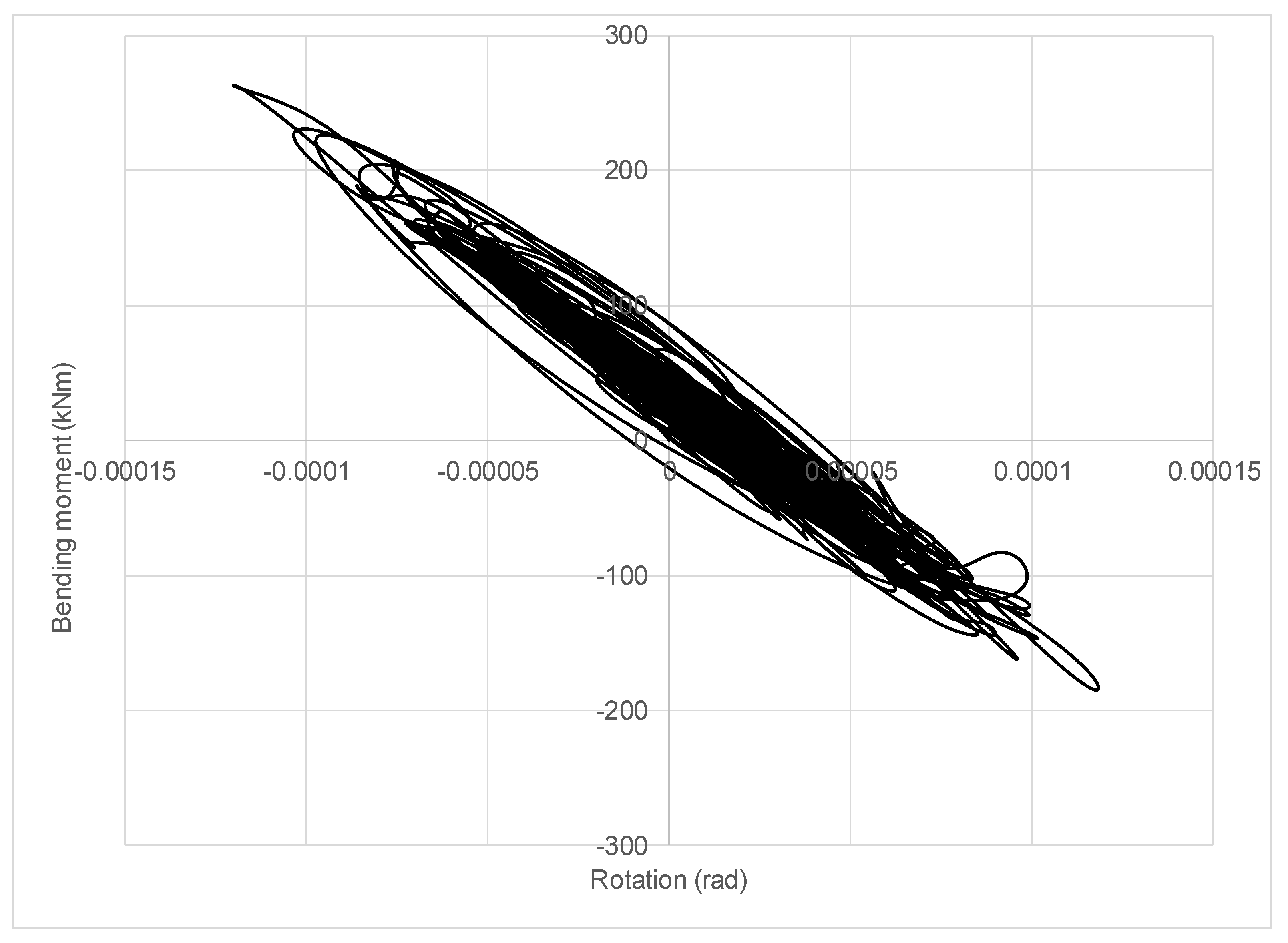
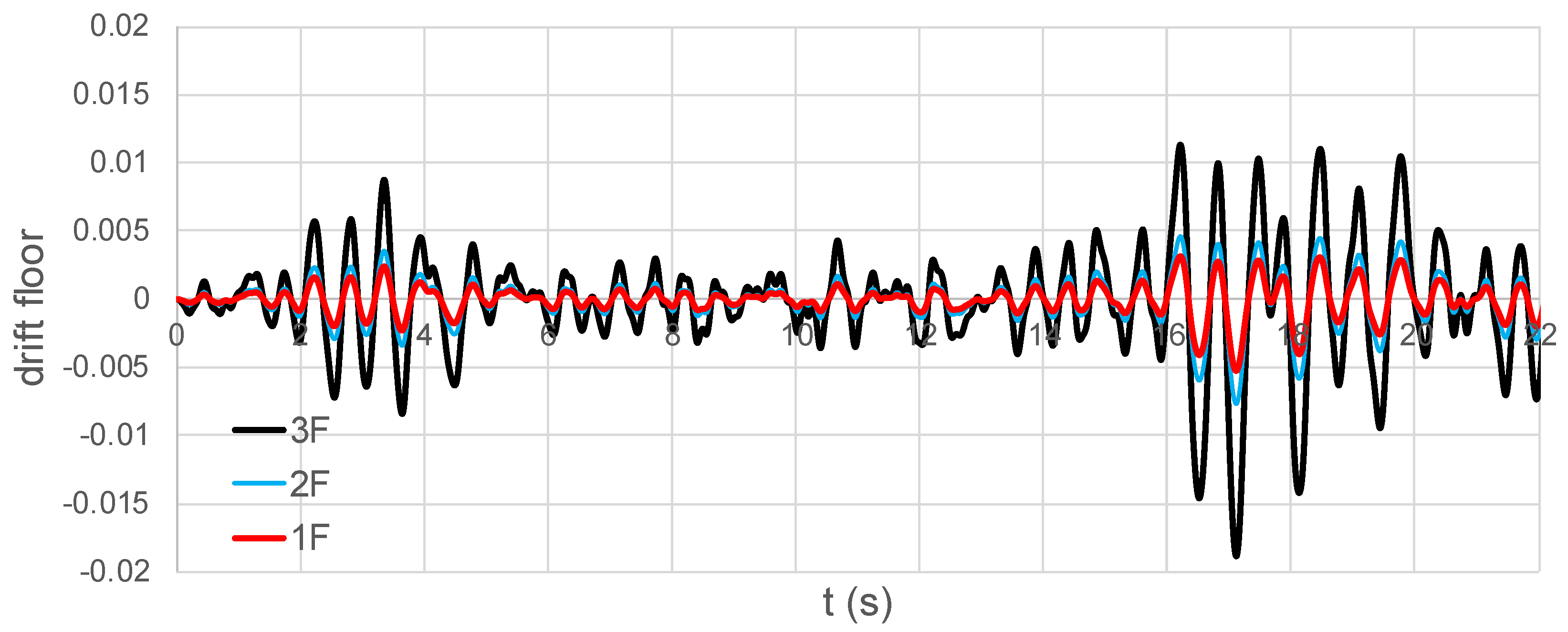
Figure 11 represents the rotation versus bending moment related to an RC column at the base of the structure. It is possible to see that the diagram presents the typical hysteretic mechanism registered during a seismic event. In particular, the values of the rotations are not significant, meaning that the rocking component of the foundation does not relevantly affect the performance of the structure, which is tied to the ground. The settlement of the foundation is not substantial as well (maximum 1.8 mm) and this is the reason for the low level of overturning moments and interstorey drifts (Figure 12), calculated as the ratio between the relative longitudinal displacement and the height of the floor from the foundation level.
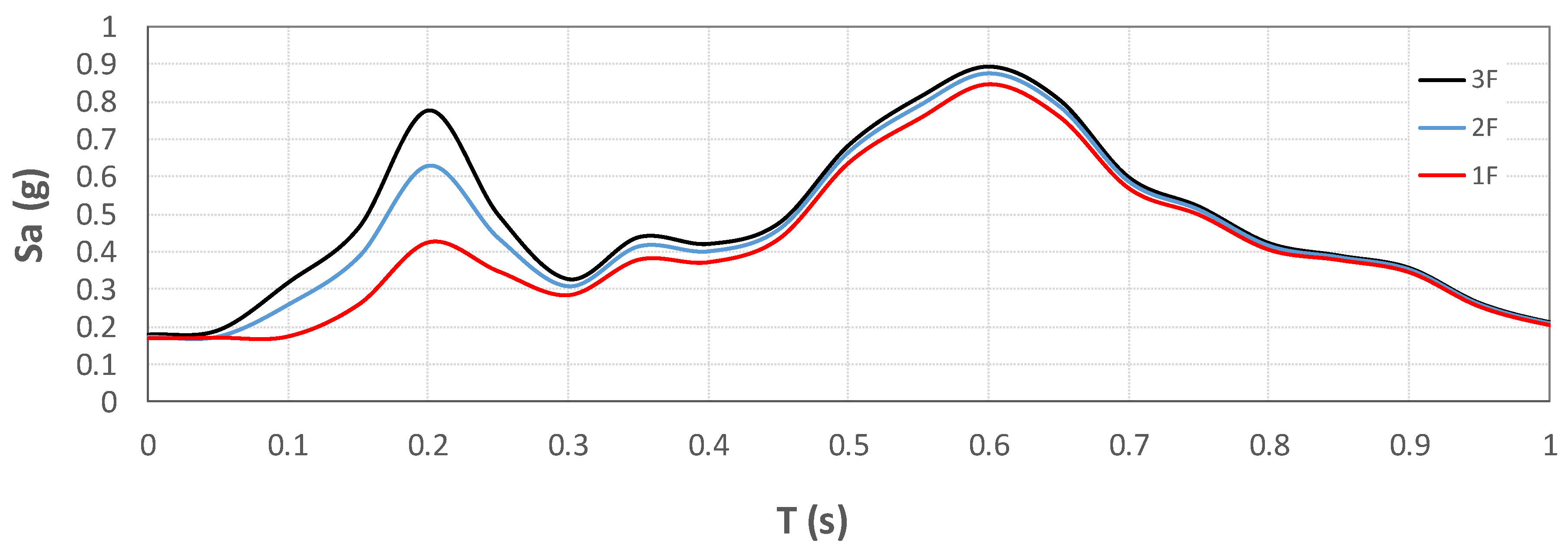
The floor spectra (5% damping), which were considered in order to assess the amplifications of the longitudinal accelerations, and thus the seismic performance of the structure, are represented in Figure 13. It is worth noticing that the peaks correspond to the fundamental period of the structure (as expected), demonstrating that the numerical model performed properly. Moreover, the accelerations increase with the height of the structure (0.426, 0.628, and 0.776 g, respectively, for floor 1, floor 2, and floor 3), with amplifications for floor 2 and floor 3 of 23.5% and 82.1% greater than those resulted for floor 1. Additionally, the significant peak related to the period of 0.6 s is noticeable, where all the structures show the same level of amplification (nearly 0.9 g). This peak corresponds to a period that is close to the fundamental period of the S2 soil, and thus may be a consequence of the mutual behavior of the soil and the structure [68].
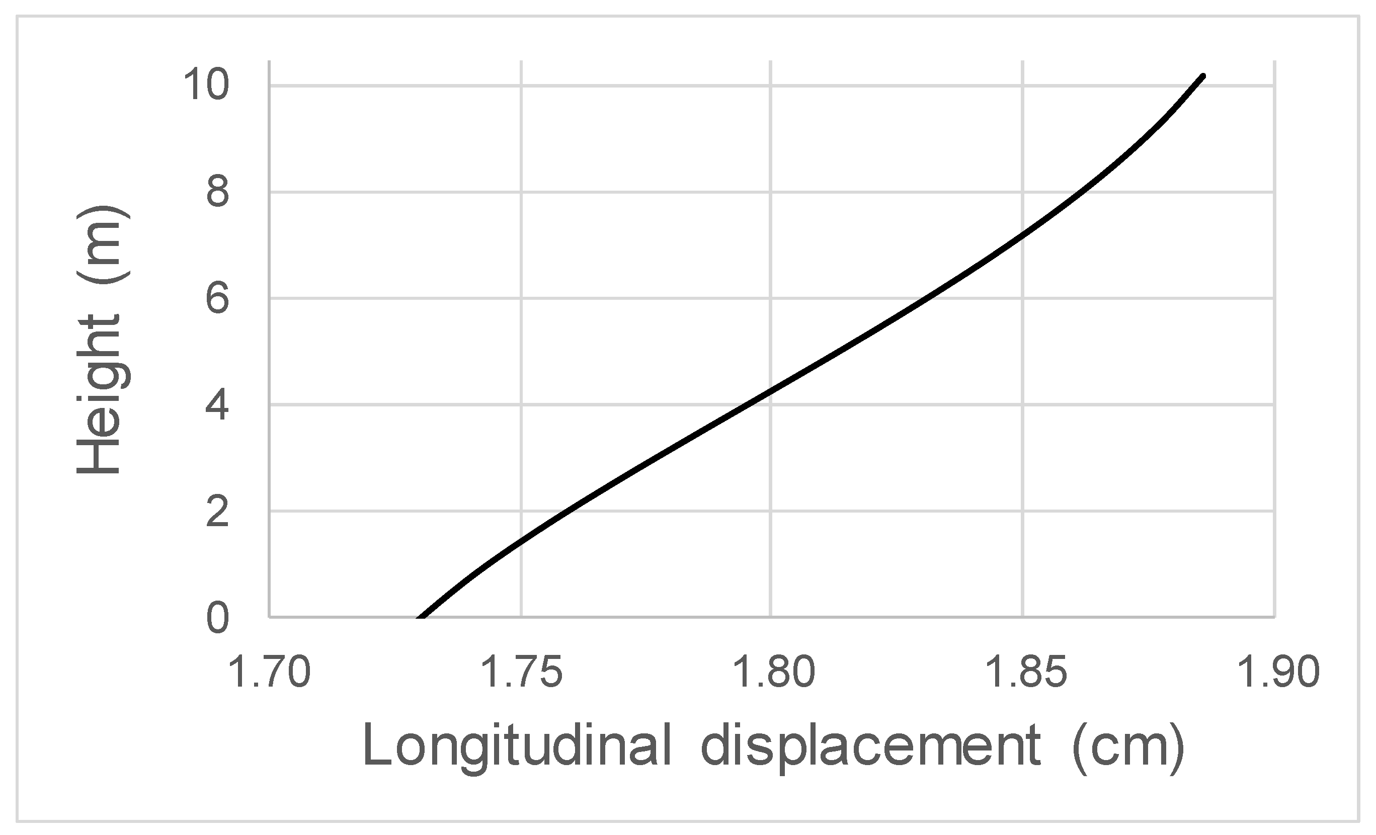
Figure 14 shows the maximum longitudinal displacements along the height of the structure. It is noticeable that the foundation maximum displacement is 1.725 cm, which means that a considerable translation occurred. In addition, since the structure is a low-rise building, the structural stiffness drives the increase in displacements along the height of the buildings and in relation to the various floors. The maximum displacement at the top of the structure is 1.885 cm, which is significant for a three-storey building in terms of structural performance.
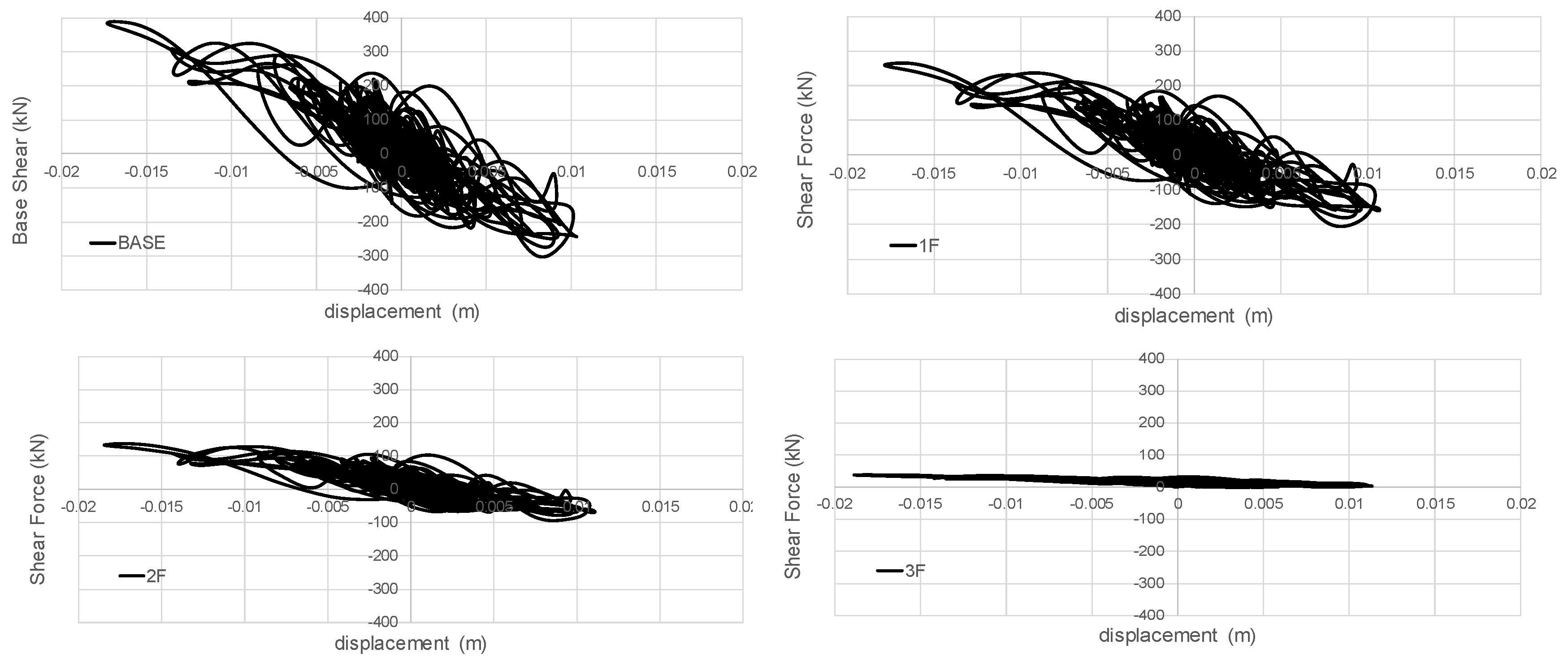
Figure 15 represents the shear forces versus longitudinal displacements for the masonry walls. These outputs are fundamental in order to define the damage conditions of the wall and to determine the potential collapse mechanism. It is worth noticing that the results are somewhat significant, demonstrating that the masonry walls are the weakest elements in the structure, as expected by the historical evidence during the 23 November 1980 Irpinia–Basilicata (southern Italy) earthquake. In particular, the maximum base shear was 390 kN and the corresponding maximum tensile stresses were approximately 65 kPa, which is close to the ultimate tensile stress. This aspect suggests that the potential damage is primarily due to the shear failure of the masonry walls.
Overall, the results demonstrate that the numerical model is in good agreement with the assumptions made so far, and thus the ground-foundation-structure system was simulated properly. The paper assessed the role of soil deformability in the amplification of accelerations, and thus its consequences on the structure. In particular, the outputs were chosen in accordance with the new approach proposed by the recent code provisions and the top floor accelerations and other significant EDP were calculated for the performed structure. In this regard, the values of the shear forces that occurred in the masonry elements show that shear failure may potentially occur in these elements, as expected and as proved by the damage that occurred during the 23 November 1980 Irpinia–Basilicata (southern Italy) earthquake.
4. Conclusions
The paper investigated the effects of soil deformability on a typical structural configuration by analyzing a 3-D soil–structure model built up with OpenSeesPL. The results are the consequence of several mechanisms known globally as the soil–structure interaction (SSI). The principal novelty of the paper consisted of proposing a model that performs detailed 3-D simulations of both the soil and the structure and assessing the structural performance in terms of displacements, drifts, and accelerations at various floors. Overall, the paper demonstrated that the soil may cause several spectral amplifications under free-field conditions (maximum amplifications: 1.66) and that a rigid low-rise building is sensitive to SSI effects, which need to be considered. Although the findings were limited to the specified conditions, they may potentially be useful to propose formulations that include SSI effects within code provisions. In this regard, future parametric numerical simulations on the response of other structural typologies and soil characteristics (e.g., water-level depth) will be performed.
Author Contributions
Please consider this paragraph that specifies the individual contributions of the authors: Conceptualization, D.F.; methodology, D.F.; software, D.M.; validation, D.M.; formal analysis, D.M. and D.F.; investigation, D.M. and D.F.; resources, D.M. and D.F.; data curation, D.M. and D.F.; writing—original draft preparation, D.M. and D.F.; writing—review and editing, D.M. and D.F.; visualization, D.M. and D.F.; supervision, D.F.; project administration, D.M. and D.F.; funding acquisition, D.M. and D.F. All authors have read and agreed to the published version of the manuscript.
Funding
This research received no external funding.
Conflicts of Interest
The authors declare no conflict of interest.
References
- Westaway, R.; Jackson, J. Surface faulting in the Southern Italian Campania-Basilicata earthquake of 23 November 1980. Nature 1984, 312, 436–438. [Google Scholar] [CrossRef]
- Cotecchia, V. Ground deformations and slope instability produced by the earthquake of 23 November 1980 in Campania and Basilicata. In Proceedings of the International Symposium Engineering Geology Problems in Seismic Areas; IAEG: Bari, Italy, 1986; Volume 5, pp. 31–100. [Google Scholar]
- Del Prete, M. Examples of mudslides hazard in Southern Apennines (Italy). Ann. Di Geofis. 1993, 36, 71–80. [Google Scholar]
- Esposito, E.; Gargiulo, A.; Iaccarino, G.; Porfido, S. Distribuzione dei fenomeni franosi riattivati dai terremoti dell’Appennino meridionale. Censimento delle frane del terremoto del 1980. In Proceedings of the Conversion International Prevention of Hydrogeological Hazards; CNR-IRPI: Torino, Italy, 1998; Volume 1, pp. 409–429. [Google Scholar]
- Pantosti, D.; Valensise, G. Source geometry and long-term behavior of the 1980 fault based on field geologic observations. Ann. Di Geofis. 1993, 36, 41–49. [Google Scholar]
- Gizzi, F.T.; Potenza, M.R.; Zotta, C. 23 November 1980 Irpinia–Basilicata earthquake (Southern Italy): Towards a full knowledge of the seismic effects. Bull. Earthq. Eng. 2012, 10, 1109–1131. [Google Scholar] [CrossRef]
- Nunziata, C.; Costa, G.; Marrara, F.; Panza, F. Validted Estimation of Response Spectra for the 1980 Irpinia Earthquake in the Eastern Area of Naples. Earthq. Spectra 2000, 16, 643–660. [Google Scholar] [CrossRef]
- Ameri, G.; Emolo, A.; Pacor, F.; Gallovič, F. Ground-Motion Simulations for the 1980 M 6.9 Irpinia Earthquake (Southern Italy) and Scenario Events. Bull. Seismol. Soc. Ameirca 2011, 101, 1136–1151. [Google Scholar] [CrossRef] [Green Version]
- Assimaki, D.; Kausel, E.; Gazetas, G. Oil-Dependent Topographic Effects: A Case Study from the 1999 Athens Earthquake. Earthq. Spectra 2005, 21, 929–966. [Google Scholar] [CrossRef]
- Seyhan, F.; Nihat, I.; Hasan, A.; Mesut, D.; Isa, V. Investigation of the soil amplification factor in the Adapari region. Bull. Eng. Geol. Environ. 2016, 75, 141–152. [Google Scholar]
- Assimaki, D.; Jeong, S. Ground-Motion observations at Hotel Montana during the 7.0 2010 Haiti Earthquake: Topography or Soil Amplification? Bull. Seismol. Soc. Ameirca 2013, 103, 2577–2590. [Google Scholar] [CrossRef] [Green Version]
- Varum, H.; Furtado, A.; Rodrigues, H.; Dias-Oliveira, J.; Vila-Pouca, N.; Arêde, A. Seismic performance of the infill masonry walls and ambient vibration tests after the Ghorka 2015, Nepal earthquake. Bull. Earthq. Eng. 2017, 15, 1185–1212. [Google Scholar] [CrossRef]
- Gautam, D.; Rodrigues, H.; Bhetwal, K.K.; Neupane, P.; Sanada, Y. Common structural and construction deficiencies of Nepalese buildings. Innov. Infrastruct. Solut. 2016, 1, 1. [Google Scholar] [CrossRef] [Green Version]
- Varum, H.; Dumaru, R.; Furtado, A.; Barbosa, A.R.; Gautam, D.; Rodrigues, H. Seismic Performance of Buildings in Nepal After the Gorkha Earthquake. In Impacts and Insights of the Gorkha Earthquake; Gautam, D., Rodrigues, H., Eds.; Elsevier: Amsterdam, The Netherlands, 2018; Chapter 3; pp. 47–63. [Google Scholar]
- Cramer, C.H. Site-specific seismic-hazard analysis that is completely probabilistic. Bull. Seismol. Soc. Am. 2003, 93, 1841–1846. [Google Scholar] [CrossRef]
- Goulet, C.A.; Stewart, J.P. Pitfalls of deterministic application of nonlinear site factors in probabilistic assessment of ground motions. Earthq. Spectra 2009, 25, 541–555. [Google Scholar] [CrossRef]
- Bazzurro, P.; Cornell, C.A. Nonlinear soil-site effects in probabilistic seismic-hazard analysis. Bull. Seismol. Soc. Am. 2004, 94, 2110–2123. [Google Scholar] [CrossRef]
- Rathje, E.M.; Pehlivan, M.; Gilbert, R.; Rodriguez-Marek, A. Incorporating Site Response into Seismic Hazard. Assessments for Critical Facilities: A Probabilistic Approach, in Perspectives on Earthquake Geotechnical Engineering; Springer International Publishing: New York, NY, USA, 2015; pp. 93–111. [Google Scholar]
- Régnier, J.; Bonilla, L.-F.; Bard, P.-Y.; Bertrand, E.; Hollender, F.; Kawase, H.; Sicilia, D.; Arduino, P.; Amorosi, A.; Asimaki, D. International benchmark on numerical simulations for 1D, nonlinear site response (PRENOLIN): Verification phase based on canonical cases. Bull. Seismol. Soc. Am. 2016, 106, 2112–2135. [Google Scholar] [CrossRef]
- Groholski, D.R.; Hashash, Y.M.; Kim, B.; Musgrove, M.; Harmon, J.; Stewart, J.P. Simplified model for small-strain nonlinearity and strength in 1D seismic site response analysis. J. Geotech. Geoenviron. Eng. 2016, 142, 4016042. [Google Scholar] [CrossRef]
- Westaway, R.; Jackson, J. The earthquake of 1980 November 23 in Campania–Basilicata (Southern Italy). Geophys. J. R. Astron. Soc. 1987, 90, 375–443. [Google Scholar] [CrossRef] [Green Version]
- Bernard, P.; Zollo, A. The Irpinia (Italy) 1980 earthquake: Detailed analysis of a complex normal faulting. J. Geophys. Res. 1989, 94, 1631–1648. [Google Scholar] [CrossRef]
- Porfido, S.; Esposito, E.; Michetti, A.M.; Blumetti, A.M.; Vittori, E.; Tranfaglia, G.; Guerrieri, L.; Ferreli, L.; Serva, L. Areal distribution of ground effects induced by strong earthquakes in the Southern Apennines (Italy). Surv. Geophys. 2002, 23, 529–562. [Google Scholar] [CrossRef]
- Porfido, S.; Alessio, G.; Gaudiosi, G.; Nappi, R.; Spiga, E. The resilience of some villages 36 years after the Irpinia-Basilicata (Southern Italy) 1980 earthquake. In Proceedings of the 4th Workshop on World Landslide Forum, Ljubljana, Slovenia, 29 May–2 June 2017. [Google Scholar]
- Pingue, F.; De Natale, G. Fault mechanism of the 40 seconds subevent of the 1980 Irpinia (Southern Italy) earthquake from levelling data. Geophys. Res. Lett. 1993, 20, 911–914. [Google Scholar] [CrossRef]
- Ascione, A.; Mazzoli, S.; Petrosino, P.; Valente, E. A decoupled kinematic model for active normal faults: Insights from the 1980, MS = 6.9 Irpinia earthquake, Southern Italy. Geol. Soc. Am. Bull. 2013, 125, 1239–1259. [Google Scholar] [CrossRef]
- Cavalieri, F.; Correia, A.A.; Crowley, H.; Pinho, R. Dynamic soil-structure interaction models for fragility characterisation of buildings with shallow foundations. Soil Dyn. Earthq. Eng. 2020, 106004. [Google Scholar] [CrossRef]
- Pitilakis, K.D.; Karapetrou, S.T.; Fotopoulou, S.D. Consideration of aging and SSI effects on seismic vulnerability assessment of RC buildings. Bull. Earthq. Eng. 2014, 12, 1755–1776. [Google Scholar] [CrossRef]
- Rajeev, P.; Tesfamariam, S. Seismic fragilities of non-ductile reinforced concrete frames with consideration of soil structure interaction. Soil Dyn. Earthq. Eng. 2012, 40, 78–86. [Google Scholar] [CrossRef]
- Anbazhagan, P.; Aditya, P.; Rashmi, H.N. Amplification based on shear wave velocity for seismic zonation: Comparison of empirical relations and site response results for shallow engineering bedrock sites. Geomech. Eng. 2011, 3, 189–206. [Google Scholar] [CrossRef]
- Rota, M.; Lai, C.G.; Strobbia, C.L. Stochastic 1D site response analysis at a site in central Italy. Soil Dyn. Earthq. Eng. 2011, 31, 626–639. [Google Scholar] [CrossRef]
- Shahri, A.A.; Esfandiyari, B.; Hamzeloo, H. Evaluation of a nonlinear seismic geotechnical site response analysis method subjected to earthquake vibrations (case study: Kerman Province, Iran). Arab. J. Geosci. 2011, 4, 1103–1116. [Google Scholar] [CrossRef]
- EC-8-3. Design of Structures for Earthquake Resistance, Part. 3: Strengthening and Repair of Buildings; European standard EN 1998-3; European Committee for Standardization (CEN): Brussels, Belgium, 2005. [Google Scholar]
- ASCE. Minimum Design Load for Buildings and Other Structures; ASCE standard no. 007-05; American Society of Civil Engineering: Reston, VA, USA, 2006. [Google Scholar]
- ASCE. Seismic Analysis of Safety-Related Nuclear Structures and Commentary; ASCE standard no. 004-98; American Society of Civil Engineering: Reston, VA, USA, 2000. [Google Scholar]
- Foti, S.; Parolai, S.; Albarello, D.; Picozzi, M. Application of Surface-Wave Methods for Seismic Site Characterization. Surv. Geophys. 2011, 32, 777–825. [Google Scholar] [CrossRef] [Green Version]
- Stokoe, K.H.; Nazarian, S.; Rix, G.J.; Sánchez-Salinero, I.; Sheu, J.C.; Mok, Y.J. In Situ Seismic Testing of Hard-to-Sample Soils by Surface Wave Method, Earthquake Engineering and Soil Dynamics II - Recent Advances in Ground Motion Evaluation; Von Thun, J.L., Ed.; ASCE Geotechnical Special Publication No. 20; ACSE: Reston, VA, USA, 1988; pp. 264–278. [Google Scholar]
- Amorosi, A.; Castellaro, S.; Mulargia, F. Single-Station Passive Seismic Stratigraphy: An inexpensive tool for quick subsurface investigations. GEOACTA 2008, 7, 29–39. [Google Scholar]
- Hobiger, M.; Wegler, U.; Shiomi, K.; Nakahara, H. Single-station cross-correlation analysis of ambient seismic noise: Application to stations in the surroundings of the 2008 Iwate-Miyagi Nairiku earthquake. Geophys. J. Int. 2014, 198, 90–109. [Google Scholar] [CrossRef] [Green Version]
- Wair, B.R.; DeJong, J.T. Guidelines for Estimation of Shear Wave Velocity Profiles; PEER Report 2012/08; Pacific Earthquake Engineering Research Center: Berkeley, CA, USA, 2012. [Google Scholar]
- Tanganelli, M.; Viti, S.; Forcellini, D.; D’Intisonante, V.; Baglione, M. Effect of soil modeling on Site Response Analysis (SRA). Alphose Zingoni, Insights and Innovations in Structural Engineering, Mechanics and Computation. In Proceedings of the SEMC 2016, Cape Town, South Africa, 5–7 September 2016; pp. 364–369, ISBN 978-1-138-02927-9. [Google Scholar]
- Viti, S.; Tanganelli, M.; D’Intinosante, V.; Baglione, M. Effects of soil characterization on the seismic input. J. Earthq. Eng. 2017, 21. [Google Scholar] [CrossRef]
- Rodriguez-Marek, A.; Kruiver, P.P.; Meijers, P.; Bommer, J.J.; Dost, B.; van Elk, J.; Doornhof, D. A regional site-response model for the Groningen gas field. Bull. Seism. Soc. Am. 2017, 107, 2067–2077. [Google Scholar] [CrossRef]
- Kruiver, P.P.; van Dedem, E.; Romijn, R.; de Lange, G.; Korff, M.; Stafleu, J.; Gunnink, J.L.; Rodriguez-Marek, A.; Bommer, J.J.; van Elk, J.; et al. An integrated shear-wave velocity model for the Groningen gas field, The Netherlands. Bull. Earthq. Eng. 2017, 15, 3555–3580. [Google Scholar] [CrossRef] [Green Version]
- Forcellini, D. Cost Assessment of isolation technique applied to a benchmark bridge with soil structure interaction. Bull. Earthq. Eng. 2017. [Google Scholar] [CrossRef]
- Forcellini, D. Seismic Assessment of a benchmark based isolated ordinary building with soil structure interaction. Bull. Earthq. Eng. 2018. [Google Scholar] [CrossRef]
- Forcellini, D. Numerical simulations of liquefaction on an ordinary building during Italian (20 May 2012) earthquake. Bull. Earthq. Eng. 2019. [Google Scholar] [CrossRef]
- Forcellini, D. Soil-structure interaction analyses of shallow-founded structures on a potential-liquefiable soil deposit. Soil Dynamics Earthq. Eng. 2020, 133, 106108. [Google Scholar] [CrossRef]
- ITACA 1.1, 2011, ITalian ACcelerometric Archive (1972-2011) version1.1. Available online: http://itaca.mi.ingv.it/ItacaNet/ (accessed on 21 April 2020).
- Zienkiewicz, O.C.; Chan, A.H.C.; Pastor, M.; Paul, D.K.; Shiomi, T. Static and dynamic behavior of soils: A rational approach to quantitative solutions: I. Fully saturated problems. Proc. R. Soc. Lond. Ser. A 1990, 429, 285–309. [Google Scholar]
- Elgamal, A.; Lu, J.; Forcellini, D. Mitigation of Liquefaction-Induced lateral deformation in sloping stratum: Three-dimensional Numerical Simulation. J. Geotech. Geoenvironmental Eng. 2009, 135, 1672–1682. [Google Scholar] [CrossRef]
- Lu, J.; Elgamal, A.; Yang, Z. OpenSeesPL: 3D Lateral Pile-Ground Interaction, User Manual, Beta 1.0. Available online: http://soilquake.net/openseespl/ (accessed on 21 April 2020).
- Mazzoni, S.; McKenna, F.; Scott, M.H.; Fenves, G.L. Open System for Earthquake Engineering Simulation, User Command-Language Manual, OpenSees version 2.0; Pacific Earthquake Engineering Research Center, University of California: Berkeley, CA, USA, 2009; Available online: http://opensees.berkeley.edu/OpenSees/manuals/usermanual (accessed on 21 April 2020).
- Yang, Z.; Elgamal, A.; Parra, E. A computational model for cyclic mobility and associated shear deformation. J. Geotech. Geoenviron. Eng. (ASCE) 2003, 129, 1119–1127. [Google Scholar] [CrossRef]
- Kramer, S.L. Geotechnical Earthquake Engineering; William, J., Ed.; International Series in Civil engineering and engineering Mechanics; Prentice-Hall: Upper Saddle River, NJ, USA, 1996. [Google Scholar]
- Madas, P.; Elnashai, A. A new passive confinement model for the analysis of concrete structures subjected to cyclic and transient dynamic loading. Earthq. Eng. Struct Dyn. 1992, 21, 409–431. [Google Scholar] [CrossRef]
- Mander, J.; Priestley, M.; Parks, R. Theoretical stress-strain model for confined concrete. J. Struct. Eng. 1988, 114, 1804–1826. [Google Scholar] [CrossRef] [Green Version]
- Menegotto, M.; Pinto, P. Method of analysis for cyclically loaded RC plane frames including changes in geometry and non-elastic behaviour of elements under combined normal force and bending. In Proceedings of the Symposium on Resistance and Ultimate Deformability of Structures Acted on by Well Defined Repeated Loads, Zurich, Switzerland, 1973. [Google Scholar]
- CIRCOLARE 2 febbraio 2009, n. 617 Istruzioni per l’applicazione delle «Nuove norme tecniche per le costruzioni» di cui al decreto ministeriale 14 gennaio 2008. Available online: http://cslp.mit.gov.it/ (accessed on 21 April 2020).
- Furtado, A.; Rodrigues, H.; Arêde, A.; Varum, H.; Grubišić, M.; Šipoš, T.K. Prediction of the earthquake response of a three-storey infilled RC structure. Eng. Struct. 2018, 171, 214–235. [Google Scholar] [CrossRef]
- Garcia, R.; Sullivan, T.J.; Della Corte, G. Development of a displacement-based design method for steel frame-RC wall buildings. J. Earthq. Eng. 2010, 14, 252–277. [Google Scholar] [CrossRef]
- Maley, T.J.; Sullivan, T.J.; Della Corte, G. Development of a displacement-based design method for steel dual systems with buckling-restrained braces and moment resisting frames. J. Earthq. Eng. 2010, 14, 106–140. [Google Scholar] [CrossRef]
- Priestley, M.J.N.; Calvi, G.M.; Kowalsky, M.J. Direct Displacement-Based Seismic Design; IUSS Press: Pavia, Italy, 2007; p. 720. [Google Scholar]
- ASCE. ASCE Standard, Minimum Design Loads for Buildings and Other Structures; ASCE/SEI 7-10; American Society of Civil Engineers: Reston, VA, USA, 2010. [Google Scholar]
- ATC-3-06. Amended Tentative Provisions for the Development of Seismic Regulations for Buildings; ATC Publication ATC 3-06, NBS Special Publication 510, NSF Publication 78-8; Applied Technology Council, US Government Printing Office: Washington, DC, USA, 1978. [Google Scholar]
- CEN. Eurocode 8: Design of Structures for Earthquake Resistance. Part. 1: General Rules, Seismic Actions and Rules for Buildings; Final Draft prEN 1998; European Committee for Standardization: Brussels, Belgium, 2003. [Google Scholar]
- CEN. Eurocode 8 Design of Structures for Earthquake Resistance. Part. 1: General Rules, Seismic Actions and Rules for Buildings; European standard EN 1998-1; European Committee for Standardization: Brussels, Belgium, 2004. [Google Scholar]
- Forcellini, D.; Gobbi, S.; Mina, D. Numerical Simulations of Ordinary Buildings with Soil Structure Interaction. Alphose Zingoni, vol. Insights and Innovations in Structural Engineering, Mechanics and Computation. In Proceedings of the SEMC 2016, Cape Town, South Africa, 5–7 September 2016; pp. 364–369, ISBN 978-1-138-02927-9. [Google Scholar]
Figure 1.
Mesh 1: free-field analysis.

Figure 2.
Mesh 2: SSI model; uniform soil layer (blue), infill (green), and foundation (yellow).

Figure 3.
Selected input motion: acceleration (a) and spectrum (b).

Figure 4.
Multi-yield surfaces in principal stress space and deviatoric plane [53].
Figure 4.
Multi-yield surfaces in principal stress space and deviatoric plane [53].

Figure 5.
Backbone curves (selected soils).

Figure 6.
Structural 3D model.

Figure 7.
Shear stress vs. shear strain relationship for Concrete02: core (a) and cover (b).

Figure 8.
Shear stress vs. shear strain relationship for Steel02 (bars).

Figure 9.
Backbone curve (infill soil).

Figure 10.
Transfer functions: S1, S2, S3, and S4 with dry and saturated conditions.


Figure 11.
Rotation vs. bending moment.

Figure 12.
Drift floor time histories.

Figure 13.
Spectra at various floors (damping ratio = 5%).

Figure 14.
Maximum longitudinal displacements.

Figure 15.
Shear forces vs. longitudinal displacements at various floors.


Table 1.
Soil characteristics.
| Soil | S1 | S2 | S3 | S4 |
|---|---|---|---|---|
| Density [Mg/m3] | 1.7 | 1.9 | 1.9 | 2.1 |
| Reference Shear Modulus [kPa] | 3.83 × 10⁴ | 4.28 × 10⁴ | 5.50 × 10⁴ | 1.32 × 10⁵ |
| Reference Bulk Modulus [kPa] | 1.50 × 10⁵ | 2.00 × 10⁵ | 2.00 × 10⁵ | 3.90 × 10⁵ |
| Shear wave velocity [m/s] | 150 | 150 | 170 | 250 |
| Soil fundamental period [s] | 0.53 | 0.53 | 0.47 | 0.32 |
| Cohesion [kPa] | 5 | 5 | 5 | 5 |
| Friction angle [°] | 27 | 29 | 35 | 40 |
| Hor. Permeability [m/s] | 1.0 × 10⁻⁷ | 1.0 × 10⁻⁷ | 1.0 × 10⁻⁷ | 1.0 × 10⁻⁷ |
| Ver. Permeability [m/s] | 1.0 × 10⁻⁷ | 1.0 × 10⁻⁷ | 1.0 × 10⁻⁷ | 1.0 × 10⁻⁷ |
Table 2.
Concrete02 (core and cover).
| Concrete02 | Core | Cover |
|---|---|---|
| Compressive strength at 28 days [kPa] | −4.630423 × 10⁴ | −2.757900 × 10⁴ |
| Strain at maximum strength [%] | −3.484000 × 10⁻³ | −2.00000 × 10⁻³ |
| Crushing strength [kPa] | −4.466062 × 10⁴ | 0 |
| Strain at crushing strength [%] | −3.572200 × 10⁻³ | −6.0000 × 10⁻³ |
| Tensile strength [kPa] | 6.482592 × 10³ | 3.861060 × 10³ |
| Tension softening stiffness [kPa] | 1.860438 × 10⁶ | 1.930530 × 10⁶ |
Table 3.
Steel02 (bars).
| Steel02 | Core | Cover |
|---|---|---|
| Yield Strength [kPa] | 4.55054 × 10⁵ | −2.757900 × 10⁴ |
| Initial elastic tangent [kPa] | 2.00000 × 10⁸ | −2.00000 × 10⁻³ |
Table 4.
Masonry characteristics [53].
Table 4.
Masonry characteristics [53].
| Diagonals | Masonry |
|---|---|
| Density [Mg/m3] | 1.8 |
| Young Modulus [kPa] | 1.50 × 10⁶ |
| Shear Modulus [kPa] | 5.00 × 10⁵ |
| Compressive strength [kPa] | 3.00 × 10³ |
| Shear strength [kPa] | 70 |
Table 5.
Structural periods.
| Models | T1 [s] | T2 [s] | T3 [s] |
|---|---|---|---|
| RC | 0.301 | 0.107 | 0.073 |
| RC with IMWs | 0.209 | 0.074 | 0.049 |
Table 6.
Foundation.
| Parameters | Concrete |
|---|---|
| Density [Mg/m3] | 2.4 |
| Reference Shear Modulus [kPa] | 1.25 × 10⁷ |
| Reference Bulk Modulus [kPa] | 1.67 × 10⁷ |
Table 7.
Infill soil characteristics.
| Soil | S1 |
|---|---|
| Density [Mg/m3] | 1.7 |
| Reference Shear Modulus [kPa] | 3.83 × 10⁴ |
| Reference Bulk Modulus [kPa] | 1.50 × 10⁵ |
| Soil fundamental period [s] | 150 |
| Cohesion [kPa] | 0.53 |
| Friction angle [°] | 5 |
| Hor. Permeability [m/s] | 27 |
| Ver. Permeability [m/s] | 1.0 × 10⁻⁷ |
© 2020 by the authors. Licensee MDPI, Basel, Switzerland. This article is an open access article distributed under the terms and conditions of the Creative Commons Attribution (CC BY) license (http://creativecommons.org/licenses/by/4.0/).
Share and Cite
MDPI and ACS Style
Mina, D.; Forcellini, D. Soil–Structure Interaction Assessment of the 23 November 1980 Irpinia-Basilicata Earthquake. Geosciences 2020, 10, 152. https://0-doi-org.brum.beds.ac.uk/10.3390/geosciences10040152
AMA Style
Mina D, Forcellini D. Soil–Structure Interaction Assessment of the 23 November 1980 Irpinia-Basilicata Earthquake. Geosciences. 2020; 10(4):152. https://0-doi-org.brum.beds.ac.uk/10.3390/geosciences10040152
Chicago/Turabian StyleMina, Daniele, and Davide Forcellini. 2020. "Soil–Structure Interaction Assessment of the 23 November 1980 Irpinia-Basilicata Earthquake" Geosciences 10, no. 4: 152. https://0-doi-org.brum.beds.ac.uk/10.3390/geosciences10040152
Note that from the first issue of 2016, this journal uses article numbers instead of page numbers. See further details here.