Landslide Susceptibility Mapping Using Integrated Methods: A Case Study in the Chittagong Hilly Areas, Bangladesh


Department of Geography, University of Tennessee, Knoxville, TN 37996, USA
*
Author to whom correspondence should be addressed.
Geosciences 2020, 10(12), 483; https://0-doi-org.brum.beds.ac.uk/10.3390/geosciences10120483
Submission received: 15 October 2020
/
Revised: 22 November 2020
/
Accepted: 25 November 2020
/
Published: 29 November 2020
Abstract
:Landslide susceptibility mapping is of critical importance to identify landslide-prone areas to reduce future landslides, causalities, and infrastructural damages. This paper presents landslide susceptibility maps at a regional scale for the Chittagong Hilly Areas (CHA), Bangladesh. The frequency ratio (FR) was integrated with the analytical hierarchy process (AHP) (FR_AHP) and logistic regression (LR) (FR_LR). A landslide inventory of 730 landslide locations and 13 landslide predisposing factors including elevation, slope, aspect, plan curvature, profile curvature, topographic wetness index (TWI), stream power index (SPI), land use/land cover, rainfall, distance from drainage network, distance from fault lines, lithology, and normalized difference vegetation index (NDVI) were used. Landslide locations were randomly split into training (80%) and validation (20%) sites to support the susceptibility analysis. A safe zone was determined based on a slope threshold for logistic regression using the exploratory data analysis. The same number of non-landslide locations were randomly selected from the safe zone to train the model (FR_LR). Success and prediction rate curves and statistical indices, including overall accuracy, were used to assess model performance. The success rate curves show that FR_LR showed the highest area under the curve (AUC) (79.46%), followed by the FR_AHP (77.15%). Statistical indices also showed that the FR_LR model gave the best performance as the overall accuracy was 0.86 for training and 0.82 for validation datasets. The prediction rate curve shows similar results. The correlation analysis shows that the landslide susceptibility maps produced by FR and FR_AHP are highly correlated (0.95). In contrast, the correlation between the maps produced by FR and FR_LR was relatively lower (0.85). It indicates that the three models are highly convergent with each other. This study’s integrated methods would be helpful for regional-scale landslide susceptibility mapping, and the landslide susceptibility maps produced would be useful for regional planning and disaster management of the CHA, Bangladesh.
1. Introduction
Landslide refers to the movement of debris, rocks, and soil under the influence of gravity [1]. It is a common phenomenon in mountainous areas [2] and accounts for 9% of the world’s disasters [3]. Landslide causes damage to infrastructure, human fatalities, and economic losses [4]. Two types of factors, predisposing and triggering ones, affect the occurrence of landslides. Predisposing factors create suitable conditions for landslides, whereas triggering factors initiate the landslides [5]. The predisposing factors of landslides include slope, elevation, aspect, curvature, geology, and land use/land cover [6]. Landslides can be triggered naturally by rapid snow melting, volcanic activity, groundwater pressure, seismic activities, wildfire, and intensive or prolonged rainfall [7,8,9,10]. Landslides can also be triggered by human activities, such as excavation, deforestation, hillslope cutting, road construction, traffic vibration, and agricultural cultivation [11]. Landslide susceptibility assessment, which shows the probability of landslides over an area, is critical to minimize the losses and deaths caused by the landslide [12,13]. A landslide susceptibility map can answer where future landslide would occur over an area but cannot answer when and the intensity. For landslide risk mapping, generally, both spatial probability, time component (when), and intensity (dimension of landslides) are considered [14]
Landslide susceptibility can be investigated using quantitative and qualitative methods. Quantitative methods determine the mathematical relationship between landslides’ occurrences and their associated predisposing factors [11]. Quantitative methods can be categorized as deterministic and probabilistic methods. In a deterministic approach, a slope safety factor, defined as the ratio of shear strength to shear stress, is commonly used to determine an area’s landslide susceptibility [7]. This approach is suitable for small areas due to the challenge of measuring the safety factor over a large area [15]. Probabilistic methods use different statistical algorithms, such as logistic regression, multiple linear regression, support vector machines, frequency ratio, and certainty factor, to determine the relationship between the presence or absence of landslides and landslide predisposing factors. Probabilistic methods can be either bivariate or multivariate [16]. Bivariate methods conduct a paired comparison of landslide occurrence with each predisposing factor. These methods usually divide each factor into a set of classes and determine the relationship between landslide occurrence and these classes [11]. The commonly used bivariate methods include the frequency ratio, the weight of evidence, fuzzy logic, evidential belief function, and statistical index [7,13]. Multivariate methods determine the relationship between landslide occurrence and multiple predisposing factors. Some commonly used multivariate methods include logistic regression, adaptive regression spline, general additive models, and decision tree. These methods can have a better performance than bivariate methods [17].
Qualitative methods depend on expert knowledge and judgment. Qualitative methods include field geomorphological analysis and index-based approaches, namely, the Analytical Hierarchy Process (AHP) and Weighted Linear Combination (WLC) [17,18]. In field geomorphological analysis, investigators carry out field investigations based on geomorphology and slope stability, and they classify the study area into several susceptibility classes [18]. Susceptibility maps produced using this method are not comparable since the judgment of the investigators may vary. Simultaneously, it is applicable for a comparatively small area and it is a time-consuming process [19,20]. In index-based approaches, investigators usually assign a weight for each predisposing factor based on their knowledge and then sum all factors based on their weights to determine the landslide susceptibility [17,18,19]. Index-based approaches are subjective but are very useful with enough landslide locations and when other data are not available. This is because quantitative methods require enough landslide locations and good quality landslide predisposing factors for susceptibility mapping [20].
The method selection for landslide susceptibility mapping depends on the scale of analysis, cost, the timeline of the project, and the inventory data [19]. Bivariate methods require an inventory covering the whole area to reduce the produced susceptibility maps’ bias towards known landslide locations [21,22]. Studies have compared different models to determine a suitable method for a specific area [15]. Machine learning methods, such as support vector machines, random forest, and gradient boosting give satisfactory accuracy for landslide susceptibility maps. However, geomorphic processes such as landslides are very complex in nature, and in recent days, vast amounts of data have become available [14]. These things bring uncertainty in the machine learning models [15]. Therefore, in recent years, hybrid models for integrating bivariate methods with multivariate, machine learning, and qualitative methods have been developed to increase the prediction capability [17,23,24,25,26]. The main aim hybrid models is to integrate a couple of weak models and improve the accuracy and reduce the uncertainty of the susceptibility map [14,15]. Some examples were shown by Althuwaynee et al. [11], who integrated a bivariate model of evidential belief function (EBF) with AHP and logistic regression to assess landslide susceptibility in Pohen and Gyeongju, South Korea. This integrated approach reduced subjectivity and increased prediction capability. Xu et al. [27] compared the integrations of the index of entropy with the logistic regression and with a support vector machine to produce landslide susceptibility maps of the Shaanxi Province of China. Their results indicated that the integration with logistic regression provided a better prediction than the integration with support vector machines. Some studies suggested that integrating bivariate and multivariate models produces better results than the integration of bivariate and machine learning models [11]. Althuwaynee et al. [12] combined the chi-squared automatic interaction detection with AHP and suggested that this integrated approach outperforms the AHP method [15].
The Chittagong Hilly Areas (CHA) is situated in the hilly region of Bangladesh (Figure 1) [28]. In the last two decades, 320 people died because of landslides in this area [29,30,31]. A significant portion of tribal people lives in this area, and their use of slash and burning methods to cultivate crops results in land degradation that may trigger additional landslides [32]. A landslide susceptibility map of the whole area would provide useful guidance for land use and regional planning in this area, specifically in urban areas and areas where cultivation agriculture is practiced.
Most landslide susceptibility maps in the CHA have been produced for cities such as the Chittagong Metropolitan Area (CMA), Cox’s Bazar, and Teknaf and Rangamati municipalities [33,34,35,36]. These cities only cover a small portion of the area. No study has been conducted to assess the landslide susceptibility of the whole region [30]. Existing studies have used qualitative methods, such as AHP and WLC, bivariate methods, such as WoE, multivariate statistical methods, such as logistic regression, and machine learning methods, such as support vector machines, to study landslide susceptibility [37,38]. No study has applied the hybrid methods to map landslide susceptibility in the CHA.
In this study, the frequency ratio (FR) method was integrated with the knowledge-based AHP (FR_AHP) and with multivariate logistic regression (LR) (FR_LR) to assess landslide susceptibility for the whole CHA. Then, the landslide susceptibility maps produced by FR, FR_AHP, and FR_LR were compared to evaluate their performances at the regional scale.
2. Study Area
The CHA include five districts: Chittagong, Cox’s Bazar, Rangamati, Bandarban, and Khagrachari, covering 20,957 km2 (Figure 1). The western part of the region, mainly in the Chittagong and Cox’s Bazar districts, is characterized by lower elevations (<50 m above sea level). The southeastern part, primarily in the Bandarban, Rangamati, and Khagrachari districts, is relatively high (>500 m above sea level) [28].
This area consists of 15 lithological formations. From these formations, the Dihing formation is the youngest tertiary sediment of loose sandstone, alternating with siltstone and shale. The Dupi Tila formation consists of sandstone, sandy clay, and siltstone [28,34,38,39]. The Boka Bil formation consists of silt shale, siltstone, sandstone, sandstone, and altered siltstone. Silt shale, siltstone, sandstone, and altered siltstone are the main components of the Boka Bil formation. Girujan Clay consists of shale and silty shale [34]. The hilly part of the study area, mainly in the western region, consists of the Tipam, Boka Bil, and Bhuban formations [28]. The Eastern part of the study is comparatively flat and contains Beach and Dune Sands, Tidal Mud, Estuarine Deposits, and Marsh Clay and Peats [34].
This area can be divided into a low hill (<300 m) and high hill ranges (>300 m) [38]. The low hill ranges consists of the Tipam, Boka Bil, and Bhuban Formations [28]. It consists of both consolidated and unconsolidated sediments. The interbedding of shale, sandstone, and siltstone is one of the characteristics of these ranges’ rock structure [39]. The high hill ranges contain Tipam Sandstone, Girujan Clay, and Bhuban Formation [34]. Landslides occur in both low and high hill ranges [27,38]. Loss of human life and infrastructural damages mainly occurred in Chittagong, Cox’s Bazar, and Rangamati districts [30,35]. The three largest cities, Chittagong Metropolitan Area (CMA), Cox’s Bazar, and Rangamati municipalities, are situated in these three districts. Due to the high population density and anthropogenic activities compared to other parts of the study area, the rate of causalities is high [30,31,35]. However, landslides also occur in the other two districts: Khagrachari and Bandarban of the study area [35].
According to the Koppen classification, CHA’s climate is characterized by a tropical monsoon climate with an annual rainfall from 2540–3777 mm [35,36]. About 80% of the landslides occur during the monsoon season (June–September) due to excessive monthly rain (about 480 mm) [38]. Fifteen percent of the rainfall occurs during the pre-monsoon (March–May) and post-monsoon (October–November) seasons. The winter season (December–February) is the driest in the study area.
3. Materials and Methods
The landslide susceptibility map quality depends on the quality and selection of the landslide inventory and predisposing factors [20]. The location, types, size, and causes of landslides are stored in a landslide inventory [5]. The selection of predisposing factors depends on the scope and availability of the data and the timeline and cost of the project [40,41,42,43,44]. A total of 730 landslide locations (Figure 1) were used in this study, which occurred from (2000–2017), with 13 casual factors for the landslide susceptibility assessment.
3.1. Landslide Inventory
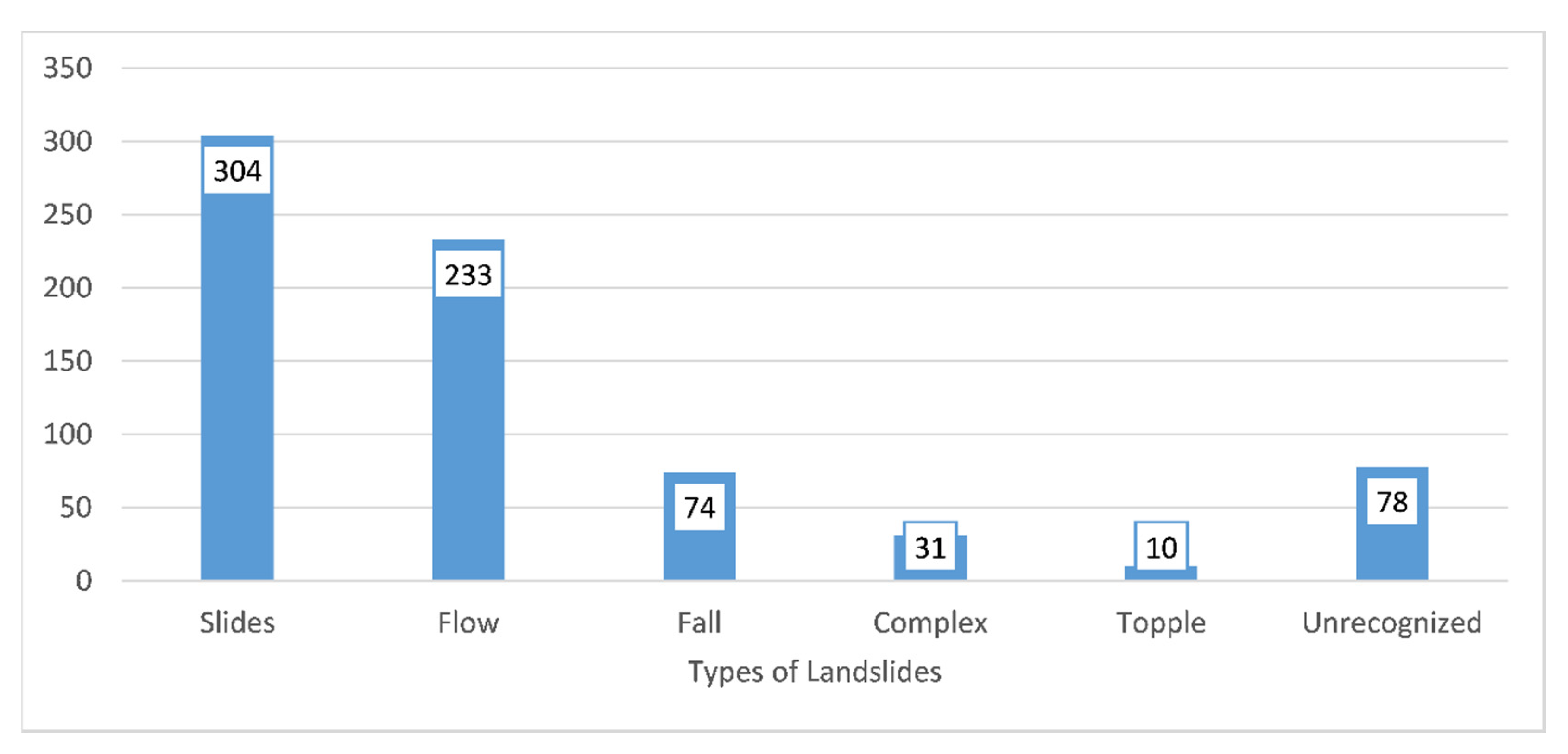
The landslide inventory was prepared using the combination of Google Earth and field mapping [36,43]. The detailed process to develop this inventory is given in Rabby and Li [31]. This inventory includes 230 landslide locations from 2000 to 2016 that were mapped in Google Earth and 548 landslides mapped during fieldwork (Figure 2) in July 2017. Field mapping was used to map landslides that occurred inaccessible areas including near the roads and settlements. In contrast, Google Earth mapping was used to map landslides in remote areas, including forests. The overlapped landslides mapped by these two methods were removed, reducing the number of landslides to 730 (Figure 1). In these 730 landslides (Figure 3), 304 are slides, 233 are flow,74 are fall, 31 are complex, 10 are topple, and 78 are unrecognized.
3.2. Predisposing Factors
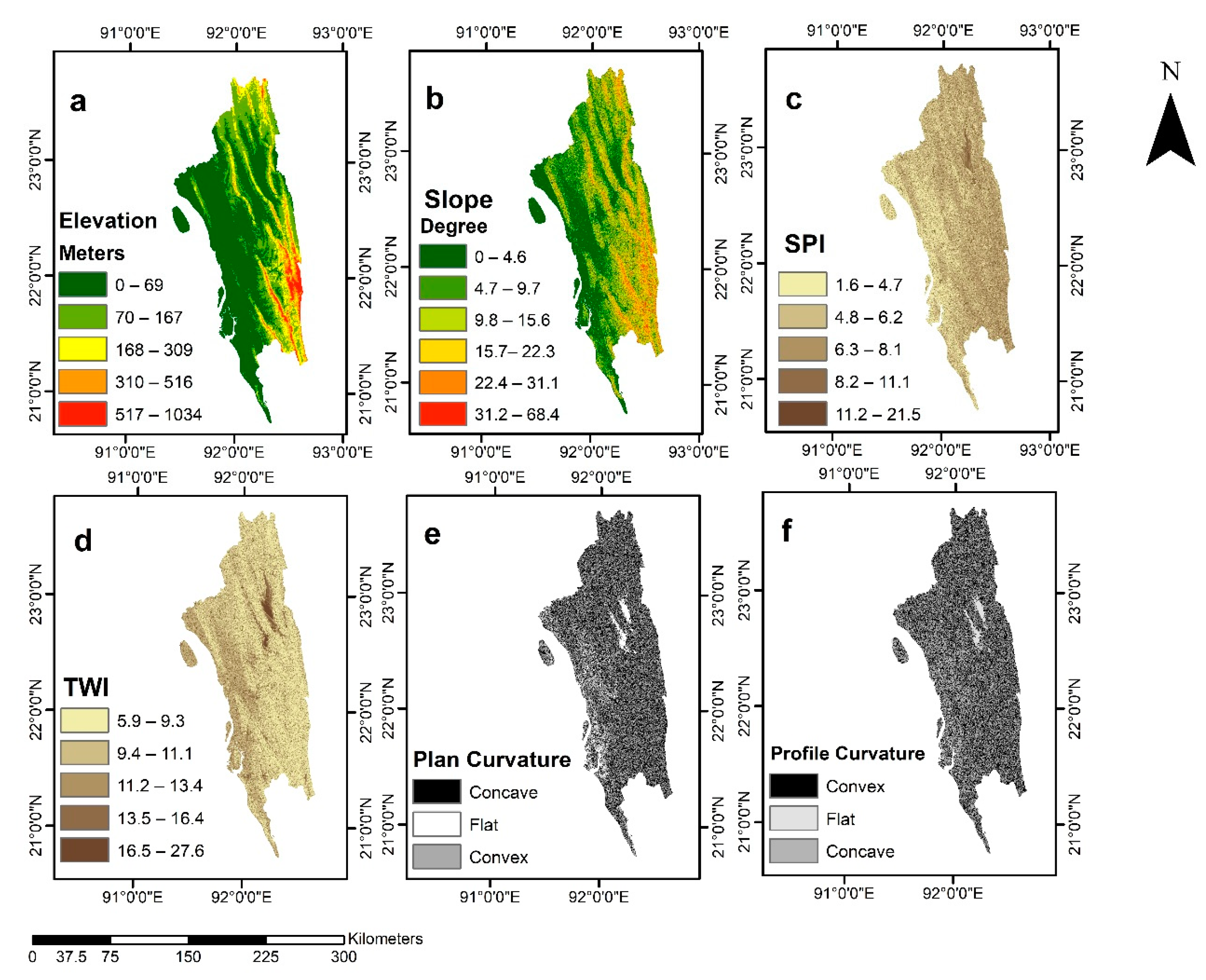
The predisposing factors used in this study include elevation, slope, Topographic Wetness Index (TWI), Stream Power Index (SPI), aspect, plan and profile curvature, Normalized Difference Vegetation Index (NDVI), distance from drainage networks, distance from fault lines, rainfall, lithology, and land use/land cover (Figure 4, Figure 5 and Figure 6).
Elevation controls temperature and vegetation. Generally, the occurrences of landslides increase with the increase of elevation before reaching a threshold elevation, where the landslide probability reduces due to rock and soil characteristics and other geotechnical parameters [41,42,43]. Elevation was obtained (Figure 4a) from the Advanced Spaceborne Thermal Emission and Reflection Radiometer (ASTER) DEM (30 m) and divided into five classes, 0–69 m, 70–167 m, 168–309 m, 310–516 m, and 517–1034 m, using the natural break method in ArcGIS 10.7. The slope is another important predisposing factor. Landslides do not occur on a gentle slope, as the shear stress is low [18]. The steeper the slope is, the higher the probability of landslides [7]. The slope raster (Figure 4b) was derived from the ASTER DEM in ArcGIS. The slope raster was then divided into five classes, 0.4–6°, 4.7–9.7°, 9.8–15.6°, 22.4–31.1°, and 31.2–68.4°, using the natural break method. The SPI represents the erosion power of the streams over an area [13]. The SPI can be determined using Equation (1) [10]:
where A is the catchment area and α is the local slope gradient corresponding to a specific cell. In our study area, floodplains and areas with lower slopes have lower SPI values (Figure 4c), whereas steeper slopes have high SPI values. The SPI values were divided into five classes, 1.6–4.7; 4.8–6.2; 6.3–8.1; 8.2–11.1; 11.2–21.5, using the natural break methods.
TWI is an index that quantifies how topography controls the hydrological processes of an area. It can be derived using Equation (2) [10]:
where A is the catchment area and α is the local slope gradient corresponding to a specific cell. TWI increases with the decrease of slope and the highest TWI value is usually on floodplains [21]. The derived TWI values were divided into five classes, 5.9–9.3, 9.4–11.1, 11.2–13.4, 13.5–16.4, and 16.5–27.6 (Figure 4d).
Curvature determines the rate of change of the slope [44]. It includes the plan curvature and profile curvature. The plan curvature is perpendicular to the maximum slope direction, whereas the profile curvature is parallel to the maximum slope [45]. The curvature affects the distribution and movement of water and sediments on the land surface [11]. The plan curvature (Figure 4e) and profile curvature (Figure 4f) were derived in ArcGIS and divided into three classes: convex, flat, and concave slopes. The probability of landslides is higher on concave slopes because soils on this slope preserve more water after a precipitation event [18].
The aspect is the orientation of the slope [7,8]. The disintegration and deterioration of materials on a slope depend on the aspect because it affects rainfall and wind [2]. The aspect raster was derived in ArcGIS and then was divide into nine classes (Figure 5a): flat (−1), north (0.22.5), northeast (22.5–67.5), east (67.5–112.5), southeast (112.5–157.5), south (157–202.5), southwest (202.5–247.5), west (247.5–292.5), northwest (292.5–337.5), and north (337.5–360).
The Normalized Difference Vegetation Index (NDVI) is an index widely used to represent vegetation and plant health [46,47,48,49,50]. Vegetation coverage protects land from erosion and landslides because the root system binds to soil and protects soil from wasting during rainfall [46]. The NDVI (Figure 5b) was derived from Landsat 8 level 2 imagery of 11 October 2017 based on Equation (3):
where IR is the infrared band and R is the red band. The NDVI ranges from −1 to 1; moderate to high NDVI (0.2–0.8) indicates vegetation and forests, a negative value usually indicates water bodies, and a low positive value (0.2 and below) represents bare land and urban areas [7,11].
Two distance-based factors were derived in ArcGIS, namely the distance from drainage (Figure 5c) and the distance from fault lines (Figure 5d), representing the proximity of drainage and fault lines on landslides.
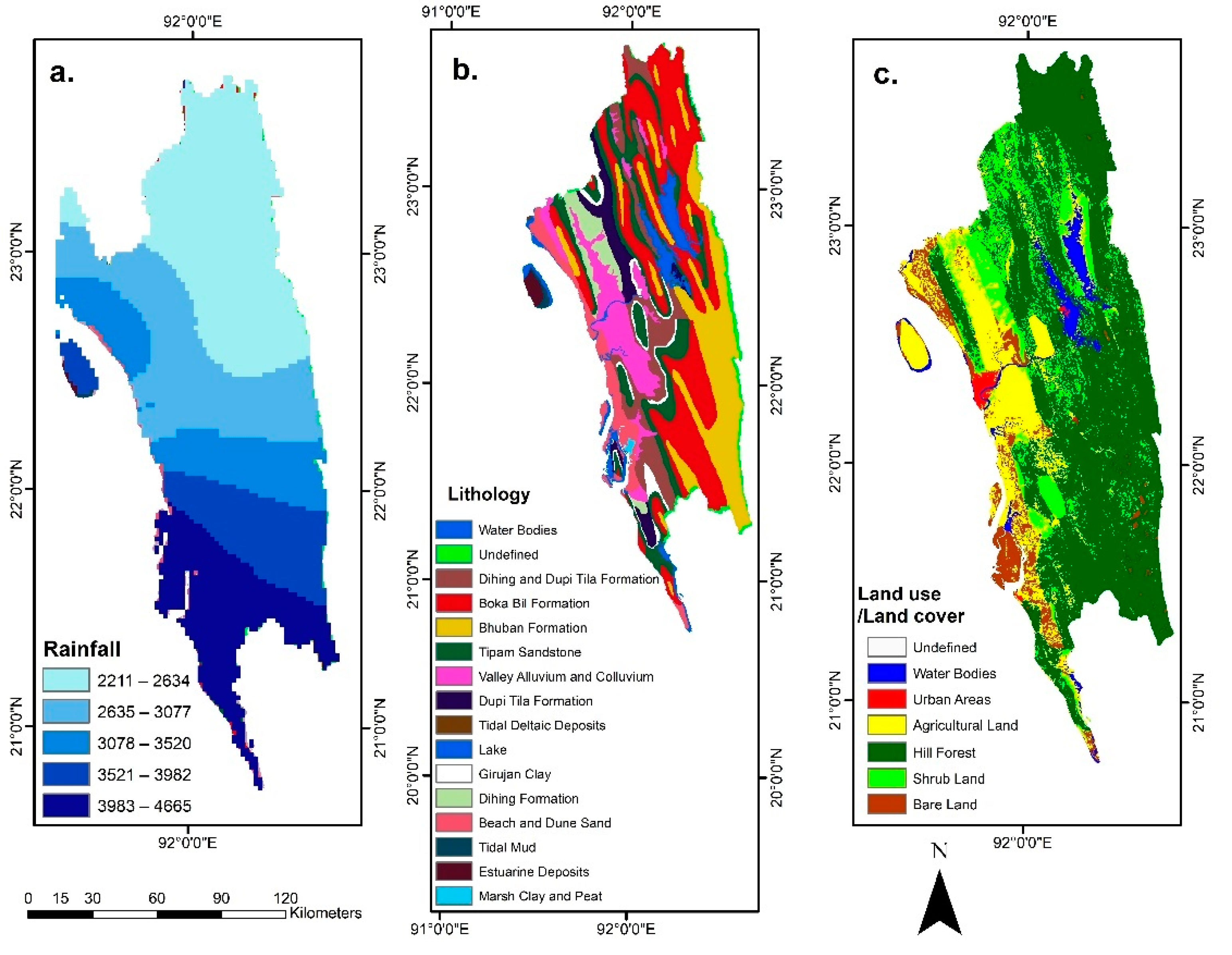
The annual rainfall data from 32 weather stations of the Bangladesh Meteorological Department (BMD) were used to produce the yearly rainfall map (Figure 6a) of the study area. Kriging tool in ArcGIS was employed to create a rainfall prediction surface map of the study area using the data of these weather stations.
Lithology is one of the most important predisposing factors of landslides [7,11]. The slope stability depends on the strength of the rocks, which depends on the local lithology. A 1:100,000 lithological map (Figure 6b) of the study area was used in this study and was provided by the1j Geological Survey of Bangladesh (GSB). Dihing and Boka Bil formations are prone to landslides because these formations have an alteration of sandstone, siltstone, and shale [25]. These formations are weak, and therefore, slope stability is comparatively low [30].
Anthropogenic activities have essential impacts on the occurrence of landslides [28]. In the study area, landslides occurred more frequently in urban areas, such as the Chittagong Hilly areas and Rangamati Sadar, than rural areas [29,30,38]. Land use/land cover map was used to represent the effects of anthropogenic activities. Six land use classes, water bodies, urban areas, agricultural land, hill forest, shrubland, and bare land (Figure 6c), were classified based on a maximum likelihood supervised classification (overall accuracy: 88.6%) of Landsat 8 images (Date of Acquisition:1 October 2017) using Erdas Imagine.
3.3. Landslide Susceptibility Mapping
In this study, three landslide susceptibility maps were generated. First, a susceptibility map was produced using the frequency ratio (FR) model, then FR was integrated with AHP and LR to create FR_AHP and FR_LR maps. FR is one of the simplest and widely used bivariate methods for landslide susceptibility mapping [48]. FR was integrated with the knowledge-based AHP and multivariate LR to improve the accuracy of landslide susceptibility mapping. A 3 × 3 (pixel) low pass filter (mean) was used to filter noise and smooth the susceptibility maps. A total of 730 landslide locations were split into training and validation datasets with an 80 to 20% ratio for model training (584: 80%) and validation (146: 20%). Most factors in this study were derived from the 30-m ASTER DEM and Landsat imagery (other than rainfall (1000 m) and lithology (1000 m)). Therefore, 30 m was used as the resolution for the landslide susceptibility mapping. This resolution was also suggested by Lee et al. [51] as the best resolution for landslide susceptibility mapping.
3.3.1. Frequency Ratio Model (FR)
The frequency ratio quantifies the association between landslide occurrence and each predisposing factor based on the conditional probability principle [52]. Each factor is first divided into a set of classes, and then the FR value for each class can be calculated using Equation (4).
where:
- -
- Nij = the number of landslide pixels within the jth subclass of factor i;
- -
- Ntotal = the total number of landslide pixels in the area;
- -
- Aij = the total number of pixels of the jth subclass of factor i;
- -
- Atotal = the total number of pixels in the study area.
The FR value ranges from 0 to ∞. A higher FR value represents a stronger association [44]. An FR value <1 indicates a lower association with landslides. For the FR calculation, each of the predisposing factors was divided into a number of classes, and Equation (4) was used to calculate the FR values for each of these classes. Therefore, the FR model gives the class-wise contribution of the predisposing factors to the landslides and cannot get the overall contribution of the predisposing factors [50].
After determining the FR values for all classes of each factor, a landslide susceptibility index (LSI) can be derived by summing up the FR values of all factors using Equation (5):
where:
LSI = FR1 + FR2 + FR3 + … + FRn,
- -
- LSI = the landslide susceptibility index at each pixel of the study area;
- -
- FR = the frequency ratio of the class of each factor at the pixel;
- -
- N = the total number of factors.
In this way, the LSI for each pixel of the study area can be determined, generating a landslide susceptibility map.
3.3.2. Integration of FR with AHP
The AHP reduces a complex decision process to a series of pairwise comparisons of influence factors based on a 1–9 scale of relative importance [53]. This scale is primarily assigned based on expert-based knowledge; thus, inheriting a certain degree of uncertainty and subjectivity [54]. The relative frequency (RF) of each sub-class of a factor using was calculated using Equation (6):
where:
- -
- RF = the relative frequency;
- -
- FRij = the frequency ratio of the jth subclass of factor i.
As an example listed in Table 1, the total FR for elevation is 3.96. The FR value for each elevation class was divided by this total FR value to derive the relative RF value.
The next step is to calculate the Prediction Rate (PR) for each predisposing factor using Equation (7):
where:
- -
- PRi = the prediction rate of factor i;
- -
- RFi_max = the maximum relative frequency of factor i;
- -
- RFi_min = the minimum relative frequency of factor i;
- -
- (RFmax − RFmin)min = the minimum difference between the maximum and minimum relative frequency among all factors.
As an example listed in Table 1, the minimum and maximum RF values for the elevation are 0.08 and 0.28, respectively. Their difference is 0.20. This value was divided by the lowest difference between the maximum and the minimum RF values among all factors (0.08). The PR value in Table 1 shows the relative importance (or weight) of each factor. These PR values were used for the pairwise comparison matrix (Table 2) to represent these factors’ relative importance. The weight for each factor was then determined using this pairwise comparison matrix and listed in Table 3.
The LSI value was derived based on each factor’s integer weight and relative frequency using Equation (8) [10,54]:
where:
- -
- RFji = the Relative Frequency of the jth subclass of factor i;
- -
- IFi = the Integer Weight of Factor i.
3.3.3. Integration of FR with LR (FR_LR)
LR determines the best fitting model to predict landslides’ presence or absence based on the predisposing factors [47]. LR models have been widely used in landslide susceptibility analysis [10,12,17,55]. The general linear equation is described as Equation (9) below:
where:
Z = ß0 + ß1X1 + ß2X2 + … + ßnXn,
- -
- Z = the linear combination of the landslide predisposing factors (Z varies from −∞ to +∞);
- -
- ßi = the coefficients of landslide predisposing factors (i = 1, 2, 3, …);
- -
- ß0 = the constant of the equation;
- -
- Xi = the predisposing factors.
A link function, Equation (10), is used in the LR model to determine the probability of the presence or absence of landslides in an area [56]:
where P = the probability of landslide occurrence ranging between 0 to 1.
This link function is combined with Equation (9) to determine the probability of landslide occurrence.
The prediction capabilities of the LR models are affected by the selection of non-landslide locations [44]. Mapping all landslides is time-consuming and sometimes impossible on a regional scale. Many mapped landslides in an inventory are near roads or settlements due to the easier accessibility [10,30,44]. It is, therefore, challenging to ensure that sampling non-landslide locations are representative of the study area, since landslide susceptibility mapping of a large area, considering all locations other than the landslides as non-landslides, affects the model’s reliability [21].
The common practice is to select the same number of non-landslide and landslide locations [57]. Studies indicate that choosing the same number of non-landslide locations from the areas where landslides were not mapped may underestimate landslide susceptibility [58,59]. Some areas can be identified as safe zones where the probability of landslides will be very low. Non-landslide locations can be selected randomly from this safe zone [44]. Exploratory data analysis can be employed to determine the safe zone [8]. In this study, the landslide locations were overlaid on the slope map to select a threshold slope, below which the landslide’s probability is very low. The landslides were ranked based on slope and it was found that 4.5° was the 10th percentile, indicating that 10% of the 730 landslides occurred in areas where the slope was ≤4.5°. To define the safe zone, a slope <4.5° was used. A total of 730 non-landslide locations were selected randomly from this zone. Selecting a safe zone based on the slope can bring bias to the FR_LR model. For example, the model will be highly dependent on the slope. At the same time, the selection of the slope threshold should be made cautiously. There is no rule in selecting the threshold. The sampling space will increase or decrease, respectively, with the slope threshold’s increase or decrease. If the sampling space is very small, most non-landslide locations will be selected from a relatively flat terrain, and the model will easily differentiate between non-landslide and landslide locations. Therefore, the training accuracy will be comparatively high. The model will not be able to identify new landslides of the validation dataset. In this study, the safe zone was selected so that it balances the sampling space and the difference between the training and validation accuracy. Since 10% of the landslide occurred in areas where the slope was <4.5°, non-landslide locations will be selected from such areas where there is a low probability of landslides but not a flat terrain where probability is almost zero. Moreover, we excluded the slope as a casual factor from the FR_LR model to reduce the bias.
In this study, land use and land cover were categorical data that may bring complexities (the other factors are continuous data), such as multicollinearity, to the LR model [17]. The categorical data were converted into continuous data based on the FR value of each land use and land cover type that we derived from the FR model [12,23]. In this way, FR was integrated with LR to generate the landslide susceptibility map. The whole dataset was divided with an 80:20 ratio into training (80%) and validation (20%) [59,60,61,62]. The multicollinearity diagnostics based on the Variance Inflation Factor (VIF) and tolerance were used, and then, the forward stepwise LR in SPSS was used for the analysis.
3.4. Validation and Comparison
Prediction and success rate curves are generally employed for accuracy assessment and model comparison [14,60]. Training data were used to generate the success rate curve, while validation data were used for the prediction rate curve [10]. The area under the curves (AUC) indicates the success rate and prediction rates. The AUC value of the success rate curve indicates the degree of fit between the model input and output, while the AUC value of the prediction rate curve indicates how well the models predict the unknown landslides [60]. The AUC value ranges from 0–1 and can be grouped into four categories: 0.50 to 0.60 (fail); 0.60–0.70 (poor); 0.70–0.80 (fair); 0.80–0.90 (good); 0.90–1.00 (excellent) [56].
It is recommended to use more than one method to validate and compare landslide susceptibility maps [41]. Therefore, in this study, three popular statistical indices: sensitivity, specificity, and overall accuracy, were used for assessing the performance [48]. Sensitivity (Table 1) is also known as the true positive rate (TPR), which means the number of landslide pixels classified correctly [62]. Specificity (Table 1) is also known as the true negative rate (TNR), which represents the number of non-landslide pixels classified correctly by the model [46]. Simultaneously, the overall accuracy (Table 1) is the ratio of truly classified landslide and non-landslide pixels and the total number of landslide and non-landslide pixels [46,63].
The Band Collection Statistics tool in ArcGIS 10.7 was also used to estimate the correlations among the landslide susceptibility mapsv [61]. These correlations indicate the level of agreement among the models [62]. This analysis generates a pairwise correlation matrix (from −1 to 1) to show the relationship between each par of the landslide susceptibility maps. Before estimating the correlations, the mean standardization of each landslide susceptibility map was carried out using the Rescale function tool in ArcGIS 10.7.
4. Results
4.1. Frequency Ratio Model
Table 1 shows FR for each of the predisposing factors. For the land use/land cover type, urban land had the highest FR value, namely 15.20, followed by shrubland, with a value of 3.15. The landslide occurrence increases with an increase of the slope. The slope class of 31.2–68.4° had the highest FR value, namely 2.55. The FR value of slopes <4.6° is less than 1, indicating a low probability of landslides.
The FR value is <1 where the altitude is above 517 m above sea level, indicating that the probability of landslides is low above this altitude in the CHA. Both the concave and convex slope had an association with the landslides (FR>1). The FR values are >1 on the northeast, south, southeast, and southwest-facing slopes, indicating a higher probability of landslides than other aspects. The landslide probability generally decreases with the increasing distance from drainage networks [41]. In this study, the FR value becomes > 1, where the distance from the drainage was <1400 m. However, the FR value becomes > 1 again in areas where the distance from drainage is >4000 m. In the NDVI, the FR value is >1, where the NDVI value is between 0.05–0.26, indicating a higher probability of landslides. This range of NDVI means bare land, built-up areas, and low-density vegetation. The FR is <1, where the NDVI value is >0.26, indicating a low probability of landslides in highly vegetated areas. In the CHA, the probability of a landslide was low (FR < 1) where rainfall was <2634 mm. The FR value was >1 in areas where the TWI value was 5.9–9.3. The probability of landslides increases with the increasing SPI value up to 8.2, and then, the FR becomes < 1, where the SPI value is > 8.2. From 15 lithological formations, Dihing and Dupi Tila (FR = 4.90) and Bhuban formations (FR = 2.10) had the highest FR values.
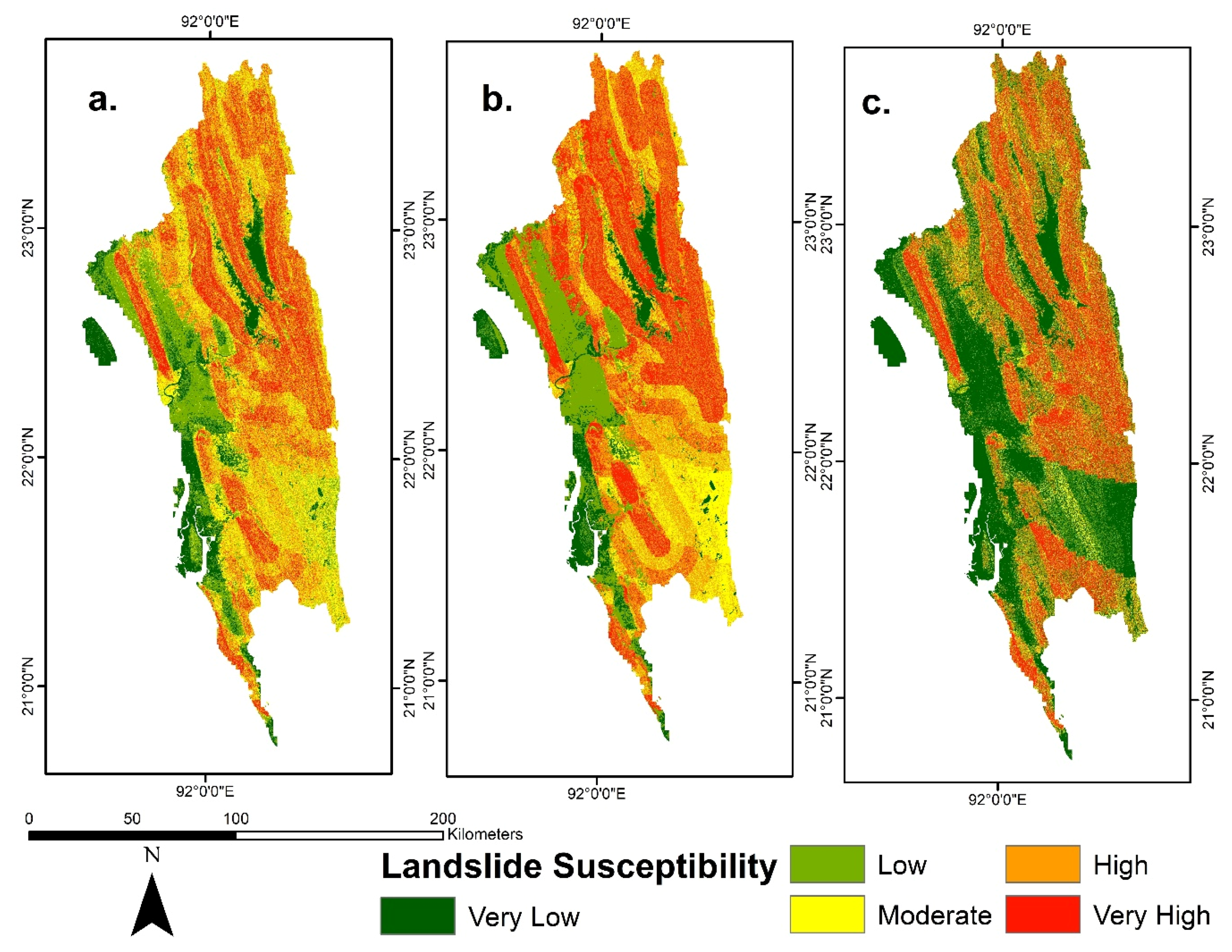
The landslide susceptibility index (LSI) at each pixel was produced by the sum of all FR values from different factors associated with this pixel based on Equation (2). The produced LSI values range from 2.7 to 59.2. These values were classified into five susceptibility classes of very low, low, moderate, high, and very high susceptibility using the natural break method for visual interpretation and validation analysis (Figure 5a). The very low and low susceptibility zones cover 25.60% of the study area, whereas the moderate, high, and very high susceptibility zones cover 24.9%, 30.70%, and 18.80% of the total area, respectively. The western part of the study area (Figure 7a) in Chittagong and Cox’s Bazar districts falls under very low to low susceptibility zones. The southeastern part of the study area in Bandarban falls under moderate susceptibility zones, with some pockets of low susceptibility zones. The northeast part of the study area in the Rangamati district falls under high to very high susceptibility zones.
4.2. Integration of FR with AHP
FR was integrated with AHP to determine each factor’s weight in terms of landslide susceptibility (Table 3 and Table 4). Table 3 shows the results of pairwise comparisons of the PR that was obtained from Table 2. The sum of each of the columns of Table 3 was used in Table 4 to calculate the eigenvalues. The integer weights are shown in Table 4. The integer weights show the contribution of each of the predisposing factors to landslides. The higher the integer weights, the higher is the importance of that predisposing factor. Table 4 shows that land use/ land cover has the highest value (95.5), indicating that this factor had a higher contribution or importance in creating a suitable condition for landslides in the study area. Distance from the fault lines (55.6), TWI (145.2), and lithology (43.2) were the next three crucial contributors to landslides. The other factors have relatively lower integer weights, indicating low contributions to landslides in the study area.
The LSI was produced using Equation (2), and it ranges from 527.8 to 2920.4. Similar to the FR model, the FR-AHP was classified to create a landslide susceptibility map into five susceptibility zones using the natural break method for visual interpretation (Figure 7b). The very low and low susceptibility zones cover 24.40% of the study area, whereas moderate, high, and very high susceptibility zones cover 26.20%, 33.50%, and 25.90% of the total area, respectively. The western part of the study area in Chittagong and Cox’s Bazar districts falls under very low to low susceptibility zones. The southeast part of the area in Bandarban was classified as a moderate susceptibility zone with some very low and low susceptibility zones.
4.3. Integration of FR with LR
Multicollinearity tests (tolerance and VIF) indicate (Table 5) that the maximum VIF value is 1.49, and the minimum tolerance value is 0.76. Since VIF values are <10 and tolerance is <0.3, 12 predisposing factors are independent and were used in the model [64].
The regression results suggest that seven predisposing factors (Table 6) were significant contributors to the presence or absence of landslides in the study area. The probability of landslides (0–1) at each pixel was derived using Equation (10) to produce the susceptibility maps.
The natural break method was used to classify the susceptibility into five visual interpretation classes (Figure 5c). In this map, 45.50% of the areas were classified as very low to low susceptibility zones, whereas moderate, high, and very high susceptibility zones covered 14.40%, 14.40%, and 25.70% of the total area, respectively. Similar to the other two maps (Figure 7a,b), the FR_AHP model (Figure 7c) classified the western part in Chittagong and Cox’s Bazar district as low to very low susceptibility zones. Unlike the other two maps, it classified the southeastern part either as a high or very high susceptibility zone. It classified the lower central part mainly in the Bandar band district as a low susceptibility zone. The northeastern part of the Rangmati district was classified as high to very high susceptibility zones.
4.4. Validation of Landslide Susceptibility Models
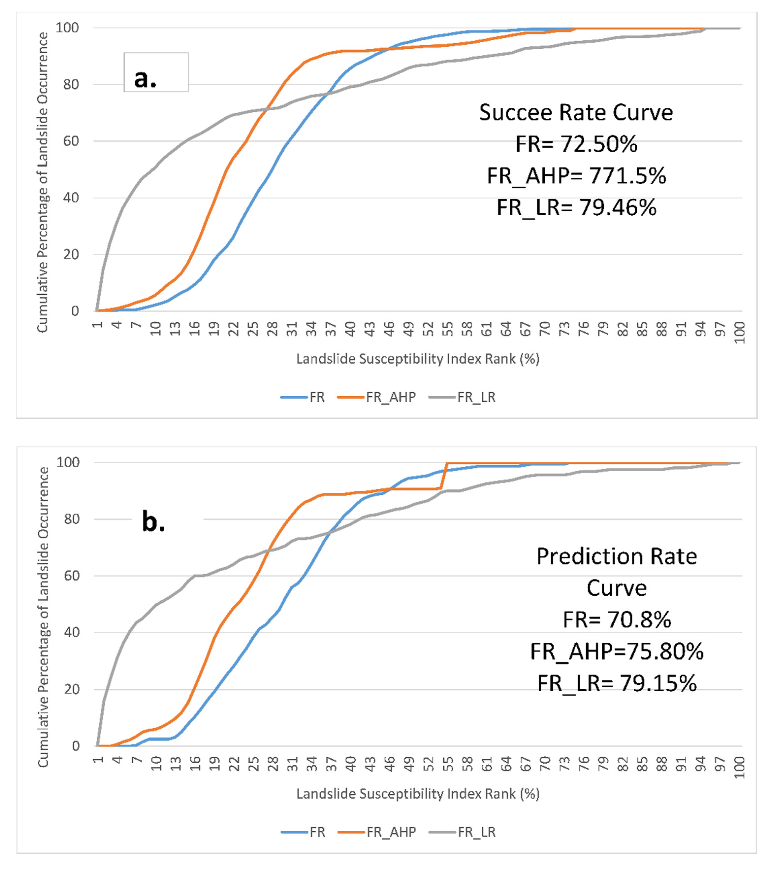
FR_LR provides the best susceptibility map, with 79.46% and 79.15% AUCs (Figure 8) of the success and prediction rate curves, respectively. FR showed the worst performance among the three models, with 72.50% and 70.80% AUCs of success and prediction rate curves, respectively. On the other hand, the success and prediction rate (Figure 8) of the FR_AHP model was 77.15% and 75.80%, respectively. This means that FR-AHP increased the success rate by 6.41% and the prediction rate by 7.10%. FR_LR increased the success rate by 9.60% and the prediction rate by 11.79%.
Statistical indices (Table 7) show similar results as the success and prediction rate curves for both training and validation datasets. FR_LR provides the best susceptibility map since the overall accuracy of training data was 0.86, and the validation data was 0.82. Integration of FR with AHP and LR increased the overall accuracy of the FR model. For FR_AHP, the increase was around 8.95% (validation dataset: Table 7) and for FR_LR the increase was around 22.38% (validation dataset: Table 7). The sensitivity of TPR of FR and FR_AHP was high compared to the FR_LR model. However, the TNR or specificity was relatively low. This is because FR and FR_AHP use the landslide locations only for training the model, whereas FR_LR requires landslide and non-landslide locations. Therefore, the false positive rate is high for both FR and FR_AHP models. This indicates that these two models overestimate the landslide susceptibility and shows some of the landslide free areas as highly susceptible to landslides. However, the integration of FR with FR_AHP increased both the TPR and TNR. This means that FR_AHP has helped to improve the performance of FR.
The correlation between FR and FR_AHP was high (0.95) (Table 8). In contrast, the correlations between FR and FR_LR and FR_AHP and FR_LR are 0.85 and 0.72 (Table 8), respectively. All these correlations were statistically significant.
From the three susceptibility maps (Figure 7), FR_LR classifies the lowest percentage of the area as either high or very high susceptibility zones. This indicates that the FR_LR model did not overestimate landslide susceptibility. At the same time, both FR and FR_AHP classified areas in the southeast of the study area as moderate susceptibility zones. The same areas were classified as low susceptibility zone by the FR_LR model. This means that both FR and FR_AHP potentially failed to differentiate the landside free zones in the southeast of the study area. This is also evident from the TNR (Table 7). In the FR_AHP model, high susceptibility zones spread around the faultlines. The FR model classified these areas as moderate susceptibility zones. FR_AHP increased the success and prediction rate by spreading the high susceptibility zones around the faultlines, and therefore, the TPR increased (Table 7). However, this did not increase the overestimation, since TNR did not improve.
5. Discussion
The objective of this study was to produce landslide susceptibility maps of the CHA, Bangladesh. The integration of FR with LR gave the highest prediction rate (79.15%). This study’s findings are consistent with previous studies, suggesting that the integration of bivariate models such as FR or evidential belief function with knowledge-based AHP and multivariate logistic regression increased the accuracy of bivariate models [10,11].
In this research, FR values (in FR model), integer weights (in FR_AHP model), and coefficients (in FR_LR) model) of significant predisposing factors were derived to quantify the effects of the predisposing factors. The FR values were > 1, where the slope was above 4.6°, and it is >1.5 above the 15.7° slope. In other studies, conducted in different regions of the world, the FR value exceeded 1.5 at around a 20° slope [51]. It indicates that other factors were responsible for the landslides at comparatively gentle slopes (<15°). For example, urban areas have the highest FR value, and cities and towns were formed in areas where the slope <20° [29,34]. In the study area, at high elevations (517–1034 m), the FR value was <1 (Table 1). In these areas, the probability of a landslide is low, and the city has similarities with other studies [18]. At higher elevations, the strength of rocks is comparatively higher than the areas with low elevation. Moreover, at high elevations, the rate of anthropogenic activities is low. Therefore, in these areas, the probability of a landslide is comparatively low [7]. The probability of a landslide was high in areas where the NDVI ranged between 0.05–0.26 (Table 1). This NDVI range indicates that areas with low vegetation density, mainly urban areas and shrublands, and areas with low vegetation are always prone to landslides [11]. Two types of land use/land cover, urban areas (FR = 15.20) and shrubland (FR = 3.15), had comparatively higher FR values than other land use/land cover types. This indicates that anthropogenic activities have an impact on the occurrence of landslides. Rahman et al. [33] found a similar relationship, where the landslide rate is higher in areas where hill-cutting occured in Chittagong Metropolitan Areas. The FR model does not deal with the interaction of the predisposing factors and does not require non-landslide locations, as it is based on landslide locations [50]. Therefore, the produced landslide susceptibility maps are often biased towards known landslide locations, and the accuracy is usually lower than the multivariate models [17]. In this study, as mentioned before, a significant number of mapped landslides were in urban areas, near roads and settlements. The FR_AHP model uses a pairwise comparison to assign weights for different factors, which increased accuracy [10]. It is based on landslide locations and does not also require non-landslide locations. The FR_AHP model also shows that predisposing factors, such as land use/land cover, TWI, NDVI, lithology, and distance from the fault lines, have high impacts on the occurrence of landslides. However, the higher integer weight of land use/land cover can be attributed to the biases that exist in the landslide inventory. In contrast, the FR_LR model considers the interaction of predisposing factors and trains the model using both landslide and non-landslide locations. The maximum likelihood estimation is used to determine the best fit model. The coefficients (Table 5) of significant predisposing factors show that some predisposing factors with very high integer weights in the FR_AHP model, such as land use/land cover, did not have a very high coefficient. It shows that the interaction of predisposing factors in a model can give different results than a model that does not consider this interaction [19]. Landslides are generally the outcome of a series of events, such as excessive rainfall and hill cutting, that involve the interaction of different factors. Therefore, the FR_LR model is more practical than the FR and FR_AHP models. Simultaneously, the FR_LR model outperforms the other two models; however, the difference between the prediction rate of FR_AHP and FR_LR is only 4.40%. All three models fall under the “fair category” [55], and FR and FR_AHP models are more straightforward than the FR_LR model. Therefore, while these three models have some practical values in urban planning and disaster management, FR_LR is a better model in terms of its practicality and performance.
The FR_LR model classified the highest percentage of areas as low or very low susceptibility zones among the three models. All three models showed the western part in the Cox’s Bazar and Chittagong district as low or very low susceptibility zones. These areas are mainly flatland near the coast, and therefore, it is evident that these areas will fall in lower susceptibility zones. However, some areas in the flatlands were erroneously classified as moderate to high susceptible zones by the LR_FR model. This type of error was reported in other studies where the logistic regression was used [32], indicating that the logistic regression model can classify the high and very high susceptible zones correctly, but some errors can be seen in the low susceptible zones [55]. Unlike FR and FR_AHP, FR_LR classified the southeastern part of the study area as either low or moderate susceptibility zones. In FR and FR_AHP models, these areas were classified as moderate susceptibility zones with some spots of low susceptibility zones. These areas can be used for development activities.
In this study, FR and FR_AHP had very high correlations. The same number of factors (13) were used for the FR and FR_AHP models, and the only difference is that FR was employed to determine the weight for each factor in the FR-AHP model, whereas all factors were treated as the same weight in the FR model. The use of different weights for factors may increase the accuracy of the landslide susceptibility map, but they are the same in principle; therefore, they produce very similar results. Compared to the correlation between FR and FR_AHP, the associations of FR to FR_LR and FR_AHP to FR_LR are lower but still statistically significant. In the FR_LR model, 12 factors (slope was excluded) were used, and the model only identified seven factors as statistically significant. In other words, only these eight factors were used to define the presence of landslides, making the FR_LR results different from the results of FR and FR-AHP. Integration of two methods can bring the problems of the two methods in the integrated one or remove one model’s problem [10]. In this study, FR and FR_AHP produced a similar type of map. However, the FR_AHP model has a higher accuracy, which it achieved by increasing the percentage of areas under high and very high susceptibility zones. The FR model has an overestimation problem since the TNR was comparatively low. Overestimation of the landslide susceptibility reduces the practical applicability of the landslide susceptibility map. A practically viable and consistent susceptibility map would classify the least percentage of area as high or very high susceptibility zones, where most of the landslides will occur [49]. The integration of FR_LR reduced the overestimation issues. It increased the accuracy and also gave a consistent and practically viable map. This is because it removed the overestimation of the susceptibility to landslides in the southeastern part of the study area. On the other hand, the integration of FR_AHP increased the TPR and therefore the overall accuracy increased, but it failed to improve TNR and was relatively low compared to FR_LR.
This study’s main limitation is that the analysis did not use some essential predisposing factors, such as soil permeability, soil depth, and types of soils, due to the unavailability of data. Landslides are mainly rainfall-triggered in the study area, and the soil permeability would help explain the landslide mechanisms. The quality of the landslide susceptibility maps depends on both the landslide inventory and predisposing factors. In this study, fieldwork covered the accessible areas, and Google Earth mapping covered the inaccessible areas. Most landslides in the fieldwork were mapped along the road or near the settlement, whereas by using Google Earth mapping, we were able to map landslides where signs of landslides can be identified in the image. Therefore, the inventory cannot be fully representative of the whole area. To get rid of this bias, we did not use predisposing factors such as the distance from the road network in the model. Generally, different types of landslides occur in various types of geology. Therefore, the preparation of separate susceptibility maps for different types of landslides gives better prediction [57]. In this study, we similarly analyzed all types of landslides. In the study area, slide and flow were the two dominant types of landslides, and we failed to identify the type of around 10% of the landslides. One way was to get rid of these landslides from the model, but this reduces its accuracy.
6. Conclusions
In this study, FR was integrated with AHP and LR to produce landslide susceptibility maps for the CHA. These models were compared, and they showed that the integration of FR with AHP and LR increases the prediction capability of a single model (FR). The AUC of the prediction rate curves shows that FR_LR was the best model, but the difference between the accuracy of FR_LR and FR_AHP is only 4.10%. However, when the practical applicability is concerned, FR_LR is better than FR_AHP.
This study is the first step for the landslide susceptibility mapping of the whole CHA. This study’s susceptibility maps are essential for the policymakers and can be used for regional development and land use planning of the CHA. The susceptibility maps identified most of the western region of the CHA as low susceptible zones. Some parts of the mid-west were classified as moderate susceptible zones. These areas can be utilized for regional development. Strict land-use planning should be implemented for the high and very high susceptible zones, where authorities and stakeholders should take precautionary measures for any development activities such as road construction.
A more representative landslide inventory of the whole study area is necessary to improve the landslide susceptibility mapping. In this study, it has been established that the integration of FR with multivariate statistical models increases the prediction capability and gives a practically viable map. The recommendation of this study is to integrate the bivariate and multivariate models for regional-scale landslide susceptibility mapping. Machine learning and deep learning methods often outperform classical models. Future studies can test the integration of bivariate models with machine learning methods, such as support vector machines, and deep learning methods, such as Artificial Neural Networks (ANN).
Author Contributions
Conceptualization, Y.W.R. and Y.L.; Methodology, Y.W.R. and Y.L.; Formal Analysis, Y.W.R.; Writing—Original Draft Preparation, Y.W.R.; Writing—Review and Editing, Y.W.R. and Y.L. All authors have read and agreed to the published version of the manuscript.
Funding
This research was funded by the McClure Scholarship program and the Penley-Tomas Fellowship program of the University of Tennessee, Knoxville, USA.
Conflicts of Interest
The authors declare no conflict of interest.
References
- Cruden, D.M.; Varnes, D.J. Landslides: Investigation and mitigation. Chapter 3-Landslide types and processes. Transp. Res. Board Spec. Rep. 1996, 247. Available online: http://onlinepubs.trb.org/Onlinepubs/sr/sr247/sr247-003.pdf (accessed on 27 November 2020).
- Roy, J.; Saha, S. Landslide susceptibility mapping using knowledge driven statistical models in Darjeeling District, West Bengal, India. Geoenvironmental Disasters 2019, 6, 11. [Google Scholar] [CrossRef] [Green Version]
- Galli, M.; Ardizzone, F.; Cardinali, M.; Guzzetti, F.; Reichenbach, P. Comparing landslide inventory maps. Geomorphology 2008, 94, 268–289. [Google Scholar] [CrossRef]
- Guzzetti, F.; Cardinali, M.; Reichenbach, P.; Cipolla, F.; Sebastiani, C.; Galli, M.; Salvati, P. Landslides triggered by the 23 November 2000 rainfall event in the Imperia Province, Western Liguria, Italy. Eng. Geol. 2004, 73, 229–245. [Google Scholar] [CrossRef]
- Guzzetti, F.; Mondini, A.C.; Cardinali, M.; Fiorucci, F.; Santangelo, M.; Chang, K.T. Landslide inventory maps: New tools for an old problem. Earth Sci. Rev. 2012, 112, 42–66. [Google Scholar] [CrossRef] [Green Version]
- Ahmed, B. Landslide Susceptibility Modelling Applying User-Defined Weighting and Data-Driven Statistical Techniques in Cox’s Bazar Municipality, Bangladesh. Nat. Hazards 2015, 79, 1707–1737. Available online: https://link.springer.com/article/10.1007/s11069-015-1922-4 (accessed on 7 March 2020). [CrossRef]
- Chen, W.; Peng, J.; Hong, H.; Shahabi, H.; Pradhan, B.; Liu, J.; Zhu, A.X.; Pei, X.; Duan, Z. Landslide susceptibility modelling using GIS-based machine learning techniques for Chongren County, Jiangxi Province. China. Sci. Total Environ. 2017, 626, 1121–1135. [Google Scholar] [CrossRef]
- Calista, M.; Miccadei, E.; Piacentini, T.; Sciarra, N. Morphostructural, Meteorological and Seismic Factors Controlling Landslides in Weak Rocks: The Case Studies of Castelnuovo and Ponzano (North East Abruzzo, Central Italy). Geosciences 2019, 9, 122. [Google Scholar] [CrossRef] [Green Version]
- Carabella, C.; Miccadei, E.; Paglia, G.; Sciarra, N. Post-Wildfire Landslide Hazard Assessment: The Case of The 2017 Montagna Del Morrone Fire (Central Apennines, Italy). Geosciences 2019, 9, 175. [Google Scholar] [CrossRef] [Green Version]
- Gariano, S.L.; Guzzetti, F. Landslides in a changing climate. Earth Sci. Rev. 2016, 162, 227–252. [Google Scholar] [CrossRef] [Green Version]
- Althuwaynee, O.F.; Pradhan, B.; Park, H.J.; Lee, J.H. A Novel Ensemble Decision Tree-Based CHi-Squared Automatic Interaction Detection (CHAID) and Multivariate Logistic Regression Models in Landslide Susceptibility Mapping. Landslides 2014, 11, 1063–1078. Available online: https://0-link-springer-com.brum.beds.ac.uk/article/10.1007/s10346-014-0466-0 (accessed on 7 March 2020). [CrossRef]
- Althuwaynee, O.F.; Pradhan, B.; Lee, S. A novel integrated model for assessing landslide susceptibility mapping using CHAID and AHP pair-wise comparison. Int. J. Remote Sens. 2016, 37, 1190–1209. [Google Scholar] [CrossRef]
- Ayalew, L.; Yamagishi, H. The application of GIS-based logistic regression for landslide susceptibility mapping in the Kakuda-Yahiko Mountains, Central Japan. Geomorphology 2005, 65, 15–31. [Google Scholar] [CrossRef]
- Dikshit, A.; Sarkar, R.; Pradhan, B.; Acharya, S.; Alamri, A.M. Spatial Landslide Risk Assessment at Phuentsholing, Bhutan. Geosciences 2020, 10, 131. [Google Scholar] [CrossRef] [Green Version]
- Merghadi, A.; Yunus, A.P.; Dou, J.; Whiteley, J.; ThaiPham, B.; Bui, D.T.; Avtar, R.; Abderrahmane, B. Machine learning methods for landslide susceptibility studies: A comparative overview of algorithm performance. Earth Sci. Rev. 2020, 207, 103225. [Google Scholar] [CrossRef]
- Zhu, A.X.; Miao, Y.; Liu, J.; Bai, S.; Zeng, C.; Ma, T.; Hong, H. A similarity-based approach to sampling absence data for landslide susceptibility mapping using data-driven methods. Catena 2019, 183, 104188. [Google Scholar] [CrossRef]
- Vakhshoori, V.; Zare, M. Landslide susceptibility mapping by comparing weight of evidence, fuzzy logic, and frequency ratio methods. Geomat. Nat. Hazards Risk 2016, 7, 1731–1752. [Google Scholar] [CrossRef]
- Yilmaz, I. Comparison of landslide susceptibility mapping methodologies for Koyulhisar, Turkey: Conditional probability, logistic regression, artificial neural networks, and support vector machine. Environ. Earth Sci. 2010, 61, 821–836. [Google Scholar] [CrossRef]
- Aleotti, P.; Robin, C. Landslide hazard assessment: Summary review and new perspectives. Bull. Eng. Geol. Environ. 1999, 58, 21–44. [Google Scholar] [CrossRef]
- Reichenbach, P.; Rossi, M.; Malamud, B.D.; Mihir, M.; Guzzetti, F. A review of statistically-based landslide susceptibility models. Earth Sci. Rev. 2018, 180, 60–91. [Google Scholar] [CrossRef]
- Yilmaz, I. Landslide susceptibility mapping using frequency ratio, logistic regression, artificial neural networks and their comparison: A case study from Kat landslides (Tokat—Turkey). Comput. Geosci. 2009, 35, 1125–1138. [Google Scholar] [CrossRef]
- Kanwal, S.; Atif, S.; Shafiq, M. GIS based landslide susceptibility mapping of northern areas of Pakistan, a case study of Shigar and Shyok Basins. Geomat. Nat. Hazards Risk 2016, 8, 348–366. [Google Scholar] [CrossRef]
- Marsala, V.; Galli, A.; Paglia, G.; Miccadei, E. Landslide Susceptibility Assessment of Mauritius Island (Indian Ocean). Geosciences 2019, 9, 493. [Google Scholar] [CrossRef] [Green Version]
- Nguyen, T.T.N.; Liu, C.-C. A New Approach Using AHP to Generate Landslide Susceptibility Maps in the Chen-Yu-Lan Watershed, Taiwan. Sensors 2019, 19, 505. [Google Scholar] [CrossRef] [PubMed] [Green Version]
- Schicker, R.; Moon, V. Comparison of bivariate and multivariate statistical approaches in landslide susceptibility mapping at a regional scale. Geomorphology 2012, 161, 40–57. [Google Scholar] [CrossRef]
- Petschko, H.; Brenning, A.; Bell, R.; Goetz, J.; Glade, T. Assessing the quality of landslide susceptibility maps–case study Lower Austria. Nat. Hazards Earth Syst. Sci. 2014, 14, 95–118. [Google Scholar] [CrossRef] [Green Version]
- Xu, L.; Coop, M.R.; Zhang, M.; Wang, G. The mechanics of a saturated silty loess and implications for landslides. Eng. Geol. 2018, 236, 29–42. [Google Scholar] [CrossRef]
- Banglapedia. Landslide, Banglapedia: National Encyclopaedia of Bangladesh 2015, Asiatic Society of Bangladesh. Available online: http://en.banglapedia.org/index.php?title=Landslide (accessed on 10 March 2018).
- Abedin, J.; Rabby, Y.W.; Hasan, I.; Akter, H. An investigation of the characteristics, causes, and consequences of June 13, 2017, landslides in Rangamati District Bangladesh. Geoenvironmental Disasters 2020, 7, 1–19. [Google Scholar] [CrossRef]
- Rabby, Y.W.; Li, Y. An integrated approach to map landslides in Chittagong Hilly Areas, Bangladesh, using Google Earth and field mapping. Landslides 2019, 16, 633–645. [Google Scholar] [CrossRef]
- Rabby, Y.W.; Li, Y. Landslide Inventory (2001–2017) of Chittagong Hilly Areas, Bangladesh. Data 2020, 5, 4. [Google Scholar] [CrossRef] [Green Version]
- Masum, K.M.; Rashid, M.M.; Jashimuddin, M.; Ara, S.J.G. Land Use Conflicts of Chittagong Hill Tracts and Indigenous Hill People as Victim in Bangladesh. J. Gen. Educ. 2011, 1, 62–71. Available online: https://www.researchgate.net/publication/235703063_Land_use_conflicts_of_Chittagong_Hill_Tracts_and_indigenous_hill_people_as_victim_in_Bangladesh. (accessed on 29 November 2018).
- Rahman, M.S.; Ahmed, B.; Huq, F.F.; Rahman, S.; Al-Hussain, T.M. Landslide Inventory in an Urban Setting in the Context of Chittagong Metropolitan, Area, Bangladesh. In Proceedings of the 3rd International conference in Civil Engineering, Chittagong, Bangladesh, 21–23 December 2016; Available online: https://www.researchgate.net/publication/308171472_Landslide_Inventory_in_an_Urban_Setting_in_the_Context_of_Chittagong_Metropolitan_Area_Bangladesh (accessed on 27 March 2017).
- Ahmed, B.; Dewan, A. Application of Bivariate and Multivariate Statistical Techniques in Landslide Susceptibility Modeling in Chittagong City Corporation. Bangladesh. Remote Sens. 2017, 9, 304. Available online: https://0-www-mdpi-com.brum.beds.ac.uk/2072-4292/9/4/304 (accessed on 7 March 2020). [CrossRef] [Green Version]
- Rahman, M.S.; Ahmed, B.; Di, L. Landslide initiation and runout susceptibility modeling in the context of hill cutting and rapid urbanization: A combined approach of weights of evidence and spatial multi-criteria. J. Mt. Sci. 2017, 14, 1919–1937. [Google Scholar] [CrossRef]
- Köppen, W.P. Grundriss der Klimakunde: 2. verb. Aufl. der Klimate der Erde; de Gruyter, W., Ed.; Borntraeger Science: Berlin, Germany, 1931; Available online: http://koeppen-geiger.vu-wien.ac.at/pdf/Koppen_1936.pdf (accessed on 27 November 2020).
- Sifa, S.F.; Mahmud, T.; Tarin, M.A.; Haque, D.M.E. Event-based landslide susceptibility mapping using weights of evidence (WoE) and modified frequency ratio (MFR) model: A case study of Rangamati district in Bangladesh. Geol. Ecol. Landsc. 2019, 1–14. [Google Scholar] [CrossRef]
- Ahmed, B.; Rahman, M.S.; Sammonds, P.; Islam, R.; Uddin, K. Application of Geospatial Technologies in Developing a Dynamic Landslide Early Warning System in a Humanitarian Context: The Rohingya Refugee Crisis in Cox’s Bazar, Bangladesh. Geomat. Nat. Hazards Risk 2020, 11, 446–468. Available online: https://0-www-tandfonline-com.brum.beds.ac.uk/doi/full/10.1080/19475705.2020.1730988 (accessed on 7 March 2020). [CrossRef]
- Brammer, H. The Physical Geography of Bangladesh; The University Press Limited: Dhaka, Bangladesh, 2012. [Google Scholar]
- Budimir, M.E.A.; Atkinson, P.M.; Lewis, H.G. A systematic review of landslide probability mapping using logistic regression. Landslides 2015, 12, 419–436. [Google Scholar] [CrossRef] [Green Version]
- Guzzetti, F. Landslide hazard assessment and risk evaluation: Limits and perspectives. In Proceedings of the 4th EGS Plinius Conference, Mallorca, Spain, 2–4 October 2002; pp. 2–4. [Google Scholar]
- Guzzetti, F.; Reichenbach, P.; Ardizzone, F.; Cardinali, M.; Galli, M. Estimating the quality of landslide susceptibility models. Geomorphology 2006, 81, 166–184. [Google Scholar] [CrossRef]
- Guzzetti, F.; Ardizzone, F.; Cardinali, M.; Rossi, M.; Valigi, D. Landslide volumes and landslide mobilization rates in Umbria, central Italy. Earth Planet. Sci. Lett. 2009, 279, 222–229. [Google Scholar] [CrossRef]
- Wang, Q.; Wang, Y.; Niu, R.; Peng, L. Integration of information theory, K-means cluster analysis and the logistic regression model for landslide susceptibility mapping in the Three Gorges Area, China. Remote Sens. 2017, 9, 938. [Google Scholar] [CrossRef] [Green Version]
- Kumar, B.P.; Babu, K.R.; Ramachandra, M.; Krupavathi, C.; Swamy, B.N.; Sreenivasulu, Y.; Rajasekhar, M. Data on identification of desertified regions in Anantapur district, Southern India by NDVI approach using remote sensing and GIS. Data Brief. 2020, 18, 105560. [Google Scholar] [CrossRef]
- Chen, W.; Shahabi, H.; Shirzadi, A.; Hong, H.; Akgun, A.; Tian, Y.; Liu, J.; Zhu, A.X.; Li, S. Novel hybrid artificial intelligence approach of bivariate statistical-methods-based kernel logistic regression classifier for landslide susceptibility modeling. Bull. Eng. Geol. Environ. 2019, 78, 4397–4419. [Google Scholar] [CrossRef]
- Chen, W.; Zhang, S.; Li, R.; Shahabi, H. Performance evaluation of the GIS-based data mining techniques of best-first decision tree, random forest, and naïve Bayes tree for landslide susceptibility modeling. Sci. Total Environ. 2018, 644, 1006–1018. [Google Scholar] [CrossRef] [PubMed]
- Islam, M.A.; Islam, M.S.; Islam, T. Landslides in Chittagong hill tracts and possible measures. In Proceedings of the International Conference on Disaster Risk Mitigation, Dhaka, Bangladesh; Available online: https://www.researchgate.net/profile/Mohammad_Islam28/publication/320014168_LANDSLIDES_IN_CHITTAGONG_HILL_TRACTS_AND_POSSIBLE_MEASURES/links/59c86a80aca272c71bc7f50d/LANDSLIDES-IN-CHITTAGONG-HILL-TRACTS-AND-POSSIBLE-MEASURES.pdf (accessed on 27 November 2020).
- Huete, K.A.; Didan, T.M. Overview of the radiometric and biophysical performance of the MODIS vegetation indices. Remote Sens. Environ. 2002, 83, 1–2. [Google Scholar] [CrossRef]
- Abedini, M.; Tulabi, S. Assessing LNRF, FR, and AHP models in landslide susceptibility mapping index: A comparative study of Nojian watershed in Lorestan province, Iran. Environ. Earth Sci. 2018, 77, 405. [Google Scholar] [CrossRef]
- Lee, S.; Ryu, J.H.; Won, J.S.; Park, H.J. Determination and application of the weights for landslide susceptibility mapping using an artificial neural network. Eng. Geol. 2004, 71, 289–302. [Google Scholar] [CrossRef]
- Lee, S.; Talib, J.A. Probabilistic landslide susceptibility and factor effect analysis. Environ. Geol. 2005, 47, 982–990. [Google Scholar] [CrossRef]
- Saaty, T.L. Decision making with the analytic hierarchy process. Int. J. Serv. Sci. 2008, 1, 83–98. [Google Scholar] [CrossRef] [Green Version]
- Ghosh, S.; Carranza, E.J.M.; Van Westen, C.J.; Jetten, V.G.; Bhattacharya, D.N. Selecting and weighting spatial predictors for empirical modeling of landslide susceptibility in the Darjeeling Himalayas (India). Geomorphology 2011, 131, 35–56. [Google Scholar] [CrossRef]
- Bonham-Carter, G.F. Geographic information systems for geoscientists-modeling with GIS. Comput. Methods Geosci. 1994, 13, 398. [Google Scholar]
- Rasyid, A.R.; Bhandary, N.P.; Yatabe, R. Performance of frequency ratio and logistic regression model in creating GIS based landslides susceptibility map at Lompobattang Mountain, Indonesia. Geoenvironmental Disasters 2016, 3, 19. [Google Scholar] [CrossRef] [Green Version]
- Regmi, A.D.; Devkota, K.C.; Yoshida, K.; Pradhan, B.; Pourghasemi, H.R.; Kumamoto, T.; Akgun, A. Application of frequency ratio, statistical index, and weights-of-evidence models and their comparison in landslide susceptibility mapping in Central Nepal Himalaya. Arab. J. Geosci. 2014, 7, 725–742. [Google Scholar] [CrossRef]
- Pellicani, R.; Argentiero, I.; Spilotro, G. GIS-based predictive models for regional-scale landslide susceptibility assessment and risk mapping along road corridors. Geomat. Nat. Hazards Risk 2017, 8, 1012–1033. [Google Scholar] [CrossRef] [Green Version]
- Shirzadi, A.; Shahabi, H.; Chapi, K.; Bui, D.T.; Pham, B.T.; Shahedi, K.; Ahmad, B.B. A comparative study between popular statistical and machine learning methods for simulating volume of landslides. Catena 2017, 157, 213–226. [Google Scholar] [CrossRef]
- Hong, H.; Liu, J.; Bui, D.T.; Pradhan, B.; Acharya, T.D.; Pham, B.T.; Zhu, A.X.; Chen, W.; Ahmad, B.B. Landslide susceptibility mapping using J48 Decision Tree with AdaBoost, Bagging and Rotation Forest ensembles in the Guangchang area (China). Catena 2018, 163, 399–413. [Google Scholar] [CrossRef]
- Environmental System Research Institute (ESRI). ArcGIS Desktop Help 10.7. Band Calculation Statistics. 2014. Available online: https://desktop.arcgis.com/en/arcmap/10.3/tools/spatial-analyst-toolbox/how-band-collection-statistics-works.htm (accessed on 7 March 2020).
- Rufat, S.; Tate, E.; Emrich, C.T.; Antolini, F. How valid are social vulnerability models? Ann. Am. Assoc. Geogr. 2019, 109, 1131–1153. [Google Scholar] [CrossRef]
- Pham, B.T.; Avand, M.; Janizadeh, S.; Phong, T.V.; Al-Ansari, N.; Ho, L.S.; Das, S.; Le, H.V.; Amini, A.; Bozchaloei, S.K.; et al. GIS Based Hybrid Computational Approaches for Flash Flood Susceptibility Assessment. Water 2020, 12, 683. [Google Scholar] [CrossRef] [Green Version]
- O’brien, R.M. A caution regarding rules of thumb for variance inflation factors. Qual. Quant. 2007, 41, 673–690. [Google Scholar] [CrossRef]
Figure 1.
Location of the study area (CHA) and the landslide and non-landslide locations.

Figure 2.
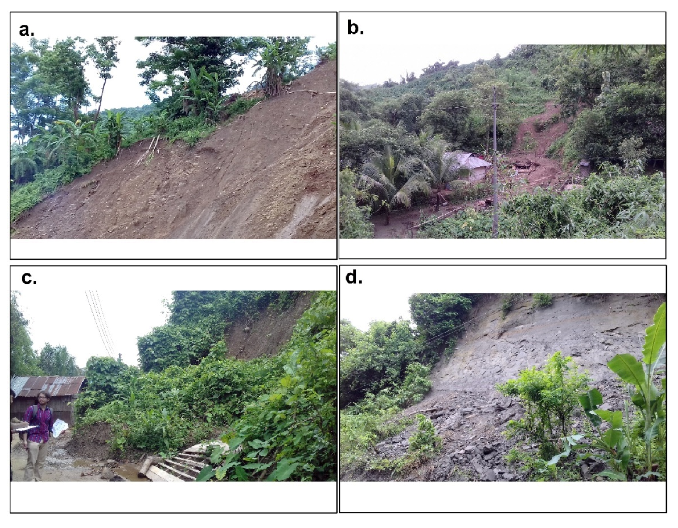
(a) Landslides damaged plantation agriculture in Bandarban; (b) Landslides damaged bamboo-made house in Rangamati; (c) Field work in Rangamati; (d) Landslides along the road in Chittagong.
Figure 2.
(a) Landslides damaged plantation agriculture in Bandarban; (b) Landslides damaged bamboo-made house in Rangamati; (c) Field work in Rangamati; (d) Landslides along the road in Chittagong.

Figure 3.
Types of Landslides in the study area.

Figure 4.
Predisposing Factors of Landslides. (a) Elevation; (b) Slope; (c) SPI; (d) TWI; (e) Plan Curvature; (f) Profile Curvature.
Figure 4.
Predisposing Factors of Landslides. (a) Elevation; (b) Slope; (c) SPI; (d) TWI; (e) Plan Curvature; (f) Profile Curvature.

Figure 5.
Predisposing Factors of Landslides. (a) Aspect; (b) NDVI; (c) Distance from Drainage Networks; (d) Distance from Fault Lines.
Figure 5.
Predisposing Factors of Landslides. (a) Aspect; (b) NDVI; (c) Distance from Drainage Networks; (d) Distance from Fault Lines.

Figure 6.
Predisposing Factors of Landslides. (a) Rainfall; (b) Lithology; (c) Land use/Land cover.

Figure 7.
Landslide susceptibility maps of the CHA, Bangladesh. (a) FR; (b) FR_AHP; (c) FR_LR.

Figure 8.
(a) Success Rate Curves; (b) Prediction Rate Curves.


Table 1.
Staistical indices usd in this study.
| Statistical Indicies | Formula |
|---|---|
| Specificity or True Positive Rate (TPR) | |
| Sensitivity or True Negative Rate (TNR) | |
| Over all Accuracy |
TP = True Positive; TN = True Negative; FN = False Negative; FP = False Positive.
Table 2.
Frequency ratios of landslide predisposing factors.
| Causal Factors | Classes | Area (%) | Landslides (%) | FR | RF | RFMin | RFMax | (RFMax−FMin) | PR |
|---|---|---|---|---|---|---|---|---|---|
| Aspect | Flat | 1.74 | 0.79 | 0.45 | 0.05 | 0.05 | 0.13 | 0.08 | 1.00 |
| North | 6.09 | 5.23 | 0.86 | 0.09 | |||||
| Northeast | 12.14 | 14.42 | 1.19 | 0.13 | |||||
| East | 12.94 | 13.15 | 1.02 | 0.11 | |||||
| Southeast | 11.49 | 12.36 | 1.08 | 0.11 | |||||
| South | 11.56 | 12.04 | 1.04 | 0.11 | |||||
| Southwest | 13.25 | 14.74 | 1.11 | 0.12 | |||||
| West | 13.82 | 10.78 | 0.78 | 0.08 | |||||
| Northwest | 11.90 | 10.94 | 0.92 | 0.10 | |||||
| North | 5.08 | 5.55 | 1.09 | 0.10 | |||||
| Elevation (m) | 0–69 | 54.75 | 61.17 | 1.12 | 0.28 | 0.08 | 0.28 | 0.20 | 2.48 |
| 70–167 | 26.45 | 27.89 | 1.05 | 0.27 | |||||
| 168–309 | 11.28 | 4.91 | 0.44 | 0.11 | |||||
| 310–516 | 5.13 | 5.23 | 1.02 | 0.26 | |||||
| 517–1034 | 2.39 | 0.79 | 0.33 | 0.08 | |||||
| Slope (°) | 0–4.6 | 35.08 | 9.98 | 0.28 | 0.03 | 0.03 | 0.30 | 0.27 | 3.30 |
| 4.7–9.7 | 25.39 | 28.21 | 1.11 | 0.13 | |||||
| 9.8–15.6 | 19.39 | 27.89 | 1.44 | 0.17 | |||||
| 15.7–22.3 | 12.04 | 19.02 | 1.58 | 0.18 | |||||
| 22.4–31.1 | 6.17 | 9.98 | 1.62 | 0.19 | |||||
| 31.2–68.4 | 1.93 | 4.91 | 2.55 | 0.30 | |||||
| SPI | 1.6–4.7 | 21.36 | 11.89 | 0.56 | 0.13 | 0.13 | 0.28 | 0.15 | 2.28 |
| 4.8–6.2 | 36.26 | 43.42 | 1.20 | 0.28 | |||||
| 6.3–8.1 | 28.88 | 33.91 | 1.17 | 0.28 | |||||
| 8.2–11.1 | 10.90 | 9.67 | 0.89 | 0.21 | |||||
| TWI | 11.2–21.5 | 2.61 | 1.11 | 0.43 | 0.10 | 0.10 | 0.46 | 0.36 | 4.52 |
| 5.9–9.3 | 37.21 | 61.65 | 1.66 | 0.46 | |||||
| 9.4–11.1 | 33.47 | 25.36 | 0.76 | 0.21 | |||||
| 11.2–13.4 | 17.97 | 8.87 | 0.49 | 0.14 | |||||
| 13.5–16.4 | 8.60 | 3.17 | 0.37 | 0.10 | |||||
| PC | Convex | 2.75 | 0.95 | 0.35 | 0.10 | 0.24 | 0.44 | 0.20 | 2.53 |
| Concave | 18.38 | 19.81 | 1.08 | 0.32 | |||||
| Flat | 58.88 | 46.75 | 0.79 | 0.24 | |||||
| PR | Convex | 22.74 | 33.44 | 1.47 | 0.44 | 0.23 | 0.43 | 0.20 | 2.41 |
| Concave | 16.72 | 24.56 | 1.47 | 0.43 | |||||
| Flat | 60.73 | 48.81 | 0.80 | 0.23 | |||||
| NDVI | Convex | 22.55 | 26.62 | 1.18 | 0.34 | 0.02 | 0.35 | 0.33 | 4.04 |
| −0.08–0.05 | 6.12 | 0.63 | 0.10 | 0.02 | |||||
| 0.05–0.18 | 13.14 | 14.44 | 1.10 | 0.25 | |||||
| 0.18–0.26 | 26.15 | 39.37 | 1.51 | 0.35 | |||||
| 0.26–0.33 | 33.87 | 30.48 | 0.90 | 0.21 | |||||
| DDN (m) | 0.33–0.50 | 20.71 | 15.08 | 0.73 | 0.17 | 0.16 | 0.25 | 0.11 | 1.20 |
| 0–1460 | 33.49 | 32.52 | 1.03 | 0.19 | |||||
| 1461–3102 | 26.67 | 29.90 | 0.89 | 0.16 | |||||
| 3103–4987 | 18.73 | 21.94 | 0.85 | 0.16 | |||||
| 4988–7542 | 16.83 | 12.25 | 1.37 | 0.25 | |||||
| DFL (m) | 7543–15,509 | 4.29 | 3.40 | 1.26 | 0.23 | 0.00 | 0.45 | 0.45 | 5.66 |
| 0–5301 | 37.70 | 61.46 | 1.63 | 0.45 | |||||
| 5302–11621 | 27.36 | 13.06 | 0.48 | 0.13 | |||||
| 11,622–19,368 | 19.60 | 20.86 | 1.06 | 0.30 | |||||
| 19,369–28,950 | 10.70 | 4.62 | 0.43 | 0.12 | |||||
| Rainfall (mm) | 28,951–51,989 | 4.64 | 0.00 | 0.00 | 0.00 | 0.00 | 0.30 | 0.30 | 3.70 |
| 2211–2634 | 32.92 | 28.93 | 0.88 | 0.18 | |||||
| 2635–3077 | 22.40 | 27.19 | 1.21 | 0.25 | |||||
| 3078–3502 | 14.55 | 20.99 | 1.44 | 0.30 | |||||
| 3521–3982 | 12.96 | 0.00 | 0.00 | 0.00 | |||||
| Land use/Land cover | 3983–4665 | 17.18 | 22.89 | 1.33 | 0.27 | 0.00 | 0.76 | 0.76 | 9.55 |
| Waterbodies | 0.80 | 0.48 | 0.60 | 0.03 | |||||
| Agricultural Land | 13.96 | 13.02 | 0.93 | 0.05 | |||||
| Hill Forest | 60.47 | 1.27 | 0.02 | 0.00 | |||||
| Shrub Land | 19.73 | 62.22 | 3.15 | 0.16 | |||||
| Urban Areas | 1.51 | 23.02 | 15.20 | 0.76 | |||||
| Bare Land | 0.03 | 0.00 | 0.00 | 0.00 | |||||
| Lithology | Undefined | 2.20 | 0.00 | 0.00 | 0.00 | 0.00 | 0.50 | 0.50 | 4.32 |
| River | 2.30 | 0.00 | 0.00 | 0.00 | |||||
| Dihing and Dupi Tila Formation | 8.50 | 42.10 | 4.90 | 0.50 | |||||
| Boka Bil Formation | 27.20 | 10.30 | 0.40 | 0.00 | |||||
| Bhuban Formation | 17.60 | 36.60 | 2.10 | 0.20 | |||||
| Tipam Sandstone | 13.80 | 0.60 | 0.00 | 0.00 | |||||
| Beach and Dune Sand | 8.80 | 1.30 | 0.10 | 0.00 | |||||
| Estuarine Deposits | 4.30 | 4.00 | 0.90 | 0.10 | |||||
| Valley Alluvium and Colluvium | 0.00 | 0.00 | 0.00 | 0.00 | |||||
| Dupi Tila Formation | 3.40 | 2.10 | 0.60 | 0.10 | |||||
| Tidal deltaic Deposits | 2.40 | 3.00 | 1.20 | 0.10 | |||||
| Lake | 3.20 | 0.00 | 0.00 | 0.00 | |||||
| Girjuan Clay | 5.20 | 0.0 | 0.00 | 0.00 | |||||
| Dihing Formation | 0.30 | 0.00 | 0.00 | 0.00 | |||||
| Tidal Mud | 0.60 | 0.00 | 0.00 | 0.00 | |||||
| Marsh Clay and Peat | 0.200 | 0.00 | 0.00 | 0.00 |
PC = Plan Curvature; PR = Profile Curvature; DDN = Distance from Drainage Network (m); DFL = Distance from Fault lines (m).
Table 3.
Pairwise wise comparison predisposing factors of landslide susceptibility.
| PR | 1.00 | 1.20 | 2.48 | 4.32 | 9.55 | 4.04 | 2.53 | 2.41 | 2.28 | 4.52 | 3.70 | 3.30 | 5.56 | |
|---|---|---|---|---|---|---|---|---|---|---|---|---|---|---|
| C | 1 | 2 | 3 | 4 | 5 | 6 | 7 | 8 | 9 | 10 | 11 | 12 | 13 | |
| 1.00 | 1 | 1.00 | 0.66 | 0.31 | 0.23 | 0.13 | 0.45 | 0.60 | 0.55 | 0.23 | 0.33 | 0.31 | 0.46 | 0.54 |
| 1.20 | 2 | 1.52 | 1.00 | 0.47 | 0.35 | 0.20 | 0.69 | 0.91 | 0.84 | 0.35 | 0.50 | 0.47 | 0.70 | 0.83 |
| 2.48 | 3 | 3.24 | 2.13 | 1.00 | 0.75 | 0.44 | 1.47 | 1.47 | 1.78 | 0.75 | 1.07 | 0.99 | 1.49 | 1.76 |
| 4.32 | 4 | 4.32 | 2.84 | 1.33 | 1.00 | 0.58 | 1.96 | 2.58 | 2.38 | 1.00 | 1.42 | 1.32 | 1.99 | 2.35 |
| 9.55 | 5 | 7.43 | 4.89 | 2.29 | 1.72 | 1.00 | 3.37 | 4.43 | 4.08 | 1.72 | 2.44 | 2.28 | 3.42 | 4.04 |
| 4.04 | 6 | 2.20 | 1.45 | 0.68 | 0.51 | 0.30 | 1.00 | 1.31 | 1.21 | 0.51 | 0.72 | 0.68 | 1.01 | 1.20 |
| 2.53 | 7 | 1.68 | 1.10 | 0.52 | 0.39 | 0.23 | 0.76 | 1.00 | 0.92 | 0.39 | 0.55 | 0.51 | 0.77 | 0.91 |
| 2.41 | 8 | 1.82 | 1.20 | 0.56 | 0.42 | 0.24 | 0.83 | 1.08 | 1.00 | 0.42 | 0.60 | 0.56 | 0.84 | 0.99 |
| 2.28 | 9 | 4.32 | 2.84 | 1.33 | 1.00 | 0.58 | 1.96 | 2.58 | 2.38 | 1.00 | 1.42 | 1.33 | 1.99 | 2.35 |
| 4.52 | 10 | 3.04 | 2.00 | 0.94 | 0.70 | 0.41 | 1.38 | 1.82 | 1.67 | 0.70 | 1.00 | 0.93 | 1.40 | 1.65 |
| 3.70 | 11 | 3.26 | 2.15 | 1.01 | 0.75 | 0.44 | 1.48 | 1.95 | 1.79 | 0.75 | 1.07 | 1.00 | 1.50 | 1.77 |
| 3.30 | 12 | 2.17 | 1.43 | 0.67 | 0.50 | 0.29 | 0.99 | 1.29 | 1.19 | 0.50 | 0.71 | 0.67 | 1.00 | 1.18 |
| 5.56 | 13 | 1.84 | 1.21 | 0.57 | 0.43 | 0.25 | 0.84 | 1.10 | 1.01 | 0.43 | 0.60 | 0.56 | 0.85 | 1.00 |
| S | 37.86 | 24.90 | 11.67 | 8.76 | 5.10 | 17.18 | 22.11 | 20.81 | 8.76 | 12.44 | 11.61 | 17.44 | 20.56 |
1 = Aspect; 2 = Distance from Drainage Network; 3 = Elevations; 4 = Geology; 5 = Land use/Land cover; 6 = NDVI; 7 = Plan Curvature; 8 = Profile Curvature; 9 = SPI; 10 = TWI; 11 = Rainfall; 12 = Slope; 13 = Distance from the Fault Lines; PR = Prediction Rate; C = Causal Factors; S = Sum.
Table 4.
Eigenvalues and integer weights of the predisposing factors of landslide susceptibility.
| PR | 1.00 | 1.20 | 2.48 | 4.32 | 9.55 | 4.04 | 2.53 | 2.41 | 2.28 | 4.52 | 3.70 | 3.30 | 5.56 | ||||
|---|---|---|---|---|---|---|---|---|---|---|---|---|---|---|---|---|---|
| C | 1 | 2 | 3 | 4 | 5 | 6 | 7 | 8 | 9 | 10 | 11 | 12 | 13 | S | FRW | IGW | |
| 1.00 | 1 | 0.02 | 0.02 | 0.02 | 0.02 | 0.01 | 0.05 | 0.02 | 0.02 | 0.02 | 0.03 | 0.02 | 0.03 | 0.0 | 0.29 | 0.02 | 10.00 |
| 1.20 | 2 | 0.03 | 0.03 | 0.02 | 0.02 | 0.01 | 0.06 | 0.03 | 0.02 | 0.03 | 0.03 | 0.03 | 0.03 | 0.0 | 0.34 | 0.03 | 12.00 |
| 2.48 | 3 | 0.05 | 0.05 | 0.04 | 0.05 | 0.03 | 0.12 | 0.06 | 0.05 | 0.05 | 0.06 | 0.05 | 0.06 | 0.0 | 0.71 | 0.05 | 24.80 |
| 4.32 | 4 | 0.09 | 0.10 | 0.07 | 0.09 | 0.05 | 0.21 | 0.10 | 0.08 | 0.09 | 0.11 | 0.09 | 0.11 | 0.0 | 1.24 | 0.09 | 43.20 |
| 9.55 | 5 | 0.20 | 0.21 | 0.15 | 0.19 | 0.11 | 0.46 | 0.22 | 0.18 | 0.20 | 0.24 | 0.21 | 0.25 | 0.1 | 2.73 | 0.20 | 95.50 |
| 4.04 | 6 | 0.09 | 0.09 | 0.07 | 0.08 | 0.05 | 0.20 | 0.09 | 0.08 | 0.09 | 0.10 | 0.09 | 0.11 | 0.0 | 1.16 | 0.09 | 40.40 |
| 2.53 | 7 | 0.05 | 0.06 | 0.04 | 0.05 | 0.03 | 0.12 | 0.06 | 0.05 | 0.05 | 0.06 | 0.05 | 0.07 | 0.0 | 0.72 | 0.05 | 25.30 |
| 2.41 | 8 | 0.05 | 0.05 | 0.04 | 0.05 | 0.03 | 0.12 | 0.06 | 0.05 | 0.05 | 0.06 | 0.05 | 0.06 | 0.0 | 0.69 | 0.05 | 24.10 |
| 2.28 | 9 | 0.05 | 0.05 | 0.04 | 0.05 | 0.03 | 0.11 | 0.05 | 0.04 | 0.05 | 0.06 | 0.05 | 0.06 | 0.0 | 0.65 | 0.05 | 22.80 |
| 4.52 | 10 | 0.10 | 0.10 | 0.07 | 0.09 | 0.05 | 0.22 | 0.10 | 0.08 | 0.10 | 0.11 | 0.10 | 0.12 | 0.0 | 1.29 | 0.10 | 45.20 |
| 3.70 | 11 | 0.08 | 0.08 | 0.06 | 0.07 | 0.04 | 0.18 | 0.09 | 0.07 | 0.08 | 0.09 | 0.08 | 0.10 | 0.0 | 1.06 | 0.08 | 37.00 |
| 3.30 | 12 | 0.07 | 0.07 | 0.05 | 0.07 | 0.04 | 0.16 | 0.08 | 0.06 | 0.07 | 0.08 | 0.07 | 0.09 | 0.0 | 0.94 | 0.07 | 33.00 |
| 5.56 | 13 | 0.12 | 0.12 | 0.09 | 0.11 | 0.07 | 0.27 | 0.13 | 0.10 | 0.12 | 0.14 | 0.12 | 0.15 | 0.1 | 1.59 | 0.12 | 55.60 |
| S | 1.00 | 1.03 | 0.76 | 0.93 | 0.56 | 2.28 | 1.08 | 0.88 | 0.99 | 1.18 | 1.02 | 1.22 | 0.5 | 13.42 |
1 = Aspect; 2 = Drainage; 3 = Elevation; 4 = Geology; 5 = Land use Land Cover; 6 = NDVI; 7 = Plan Curvature; 8 = Profile Curvature; 9 = SPI; 10 = TWI; 11 = Rainfall; 12 = Slope; 13 = Distance from Fault lines; PR = Prediction Rate; C = Causal Factors; S = Sum; IGW = Integer Weight.
Table 5.
Collinearity Statistics.
| Predisposing Factors | VIF | Tolerance |
|---|---|---|
| Distance from Drainage Networks | 1.03 | 0.98 |
| TWI | 1.36 | 0.74 |
| SPI | 1.11 | 0.90 |
| Profile Curvature | 1.20 | 0.83 |
| Plan Curvature | 1.21 | 0.82 |
| NDVI | 1.08 | 0.93 |
| Land use/Land cover | 1.49 | 0.88 |
| Distance from Fault lines | 1.14 | 0.88 |
| Elevation | 1.05 | 0.95 |
| Aspect | 1.03 | 0.97 |
| Rainfall | 1.04 | 0.96 |
| Lithology | 1.31 | 0.77 |
Table 6.
Results of Logistic Regression.
| Predisposing Factors | B | Standard Error | Sigificance | Exp(B) |
|---|---|---|---|---|
| TWI | 0.09 | 0.01 | 0.00 | 1.10 |
| SPI | 0.11 | 0.01 | 0.00 | 1.15 |
| Rainfall | 0.12 | 0.02 | 0.00 | 1.16 |
| Plan Curvature | 0.03 | 0.01 | 0.01 | 1.06 |
| NDVI | 0.05 | 0.01 | 0.00 | 1.08 |
| Land use Land Cover | 0.02 | 0.01 | 0.00 | 1.03 |
| Distance from Fault lines | 0.05 | 0.01 | 0.00 | 1.07 |
| Lithology | 0.08 | 0.01 | 1.11 | |
| Constant | −13.85 | 0.93 | 0.00 | 0.00 |
Table 7.
Results of the statistical indices of the landslide susceptibility maps.
| Training Data Set | Validation Data Set | |||||
|---|---|---|---|---|---|---|
| Statistical Indices | Statistical Indices | |||||
| Model Name | True Positive Rate (TPR) | True Negative Rate (TNR) | Overall Accuracy | True Positive Rate (TPR) | True Negative Rate (TNR) | Overall Accuracy |
| FR | 0.93 | 0.49 | 0.71 | 0.90 | 0.45 | 0.67 |
| FR_AHP | 0.95 | 0.59 | 0.77 | 0.95 | 0.52 | 0.75 |
| FR_LR | 0.87 | 0.86 | 0.86 | 0.85 | 0.80 | 0.82 |
Table 8.
Overall correlation between landslide susceptibility models.
| Model Name | FR | FR_AHP | FR_LR |
|---|---|---|---|
| FR | 1.00 | 0.95 | 0.85 |
| FR_AHP | 0.95 | 1.00 | 0.72 |
| FR_LR | 0.85 | 0.72 | 1.00 |
Publisher’s Note: MDPI stays neutral with regard to jurisdictional claims in published maps and institutional affiliations. |
© 2020 by the authors. Licensee MDPI, Basel, Switzerland. This article is an open access article distributed under the terms and conditions of the Creative Commons Attribution (CC BY) license (http://creativecommons.org/licenses/by/4.0/).
Share and Cite
MDPI and ACS Style
Rabby, Y.W.; Li, Y. Landslide Susceptibility Mapping Using Integrated Methods: A Case Study in the Chittagong Hilly Areas, Bangladesh. Geosciences 2020, 10, 483. https://0-doi-org.brum.beds.ac.uk/10.3390/geosciences10120483
AMA Style
Rabby YW, Li Y. Landslide Susceptibility Mapping Using Integrated Methods: A Case Study in the Chittagong Hilly Areas, Bangladesh. Geosciences. 2020; 10(12):483. https://0-doi-org.brum.beds.ac.uk/10.3390/geosciences10120483
Chicago/Turabian StyleRabby, Yasin Wahid, and Yingkui Li. 2020. "Landslide Susceptibility Mapping Using Integrated Methods: A Case Study in the Chittagong Hilly Areas, Bangladesh" Geosciences 10, no. 12: 483. https://0-doi-org.brum.beds.ac.uk/10.3390/geosciences10120483
Note that from the first issue of 2016, this journal uses article numbers instead of page numbers. See further details here.