Article

The Use of Polyurethane Injection as a Geotechnical Seismic Isolation Method in Large-Scale Applications: A Numerical Study

by
Michele Placido Antonio Gatto
1,
Valentina Lentini
2,*,
Francesco Castelli
2,
Lorella Montrasio
1 and
Davide Grassi
3
1
Department of Engineering and Architecture, University of Parma, Parco Area delle Scienze, 181/A, 43121 Parma, Italy
2
Faculty of Engineering and Architecture, University Kore of Enna, Viale delle Olimpiadi, 94100 Enna, Italy
3
Master Builders Solutions Italia Spa, Strada Vicinale delle Corti, 21, 31100 Treviso, Italy
*
Author to whom correspondence should be addressed.
Submission received: 28 February 2021 / Revised: 20 April 2021 / Accepted: 28 April 2021 / Published: 4 May 2021
(This article belongs to the Special Issue Numerical Modeling in Geotechnical Engineering)

Abstract

:
This paper analyses the effect of polyurethane injections on the seismic surficial response of cohesionless soils. For this purpose, dynamic finite element numerical analyses were performed through GiD + OpenSees. Both the soil and the composite material, resulted after the expansion of the injected polyurethane, are modelled with a nonlinear hysteretic constitutive model. Based on the polyurethane percentage, a homogenisation of the characteristics was considered for the composite material: linear for density and damping, and exponential (experimentally calibrated) for the stiffness. An expansion coefficient quantifies how much the injected polyurethane expands: three expansion coefficients were considered, each of them related to a different polyurethane density. For the evaluation of the foam stiffness, a linear stiffness–density correlation was used, derived after impact tests. Results showed that polyurethane reduces the surficial accelerations proportionally to the ratio of its seismic impedance and volumetric percentage with respect to the soil seismic impedance and total volume. This is a preliminary indication for the design of polyurethane injections in cohesionless soils for seismic acceleration reduction.

1. Introduction

Every year, earthquakes are one of the natural events responsible for both life and economic loss. In a certain time interval, the seismic risk quantifies the damage expected after an earthquake, whereby it combines the effects of seismic hazard, vulnerability and exposition. The effects of an earthquake depend on its energy and occurrence frequency (seismic hazard); for a certain intensity, structures designed inadequately, built with poor materials or subjected to poor maintenance over the years suffer the worst consequences (vulnerability). Finally, damage to people and things are greater depending on their exposition. Many seismic events have been responsible for extensive damage, and among the most recent was the 2015 Gorkha earthquake, which occurred on 25 April 2015 in Nepal [1]. Gautam and Rodrigues [2] report 8790 lives lost and $7 billion in damages, as quantified by the National Planning Commission of Nepal.
The scientific interest in the seismic risk mitigation involves several areas: engineering, as well as organisational and socio-economic, if you think about the risk management plans, which include strategies related to the seismic risk evaluation itself [3,4,5,6]. Although earthquakes cause deaths and disruption because of their secondary effects, such as landslides, tsunamis or fires, the greatest losses of both human life and property result when man-made structures collapse, due to ground motion. As a consequence, the most effective way to reduce earthquake damage is through the design and the building of earthquake-resistant structures.
From an engineering point of view, the main research attention is therefore paid to the development of structural interventions, finalised to reduce the structural vulnerability or intervening indirectly to the seismic hazard, so that a “modified” and reduced ground motion would act on the structure [7,8,9,10,11,12,13,14,15,16]. In some cases, these techniques are difficult to be applied to existing buildings or, if possible, they are invasive, and this aspect is quite relevant for buildings of historical and artistic heritage.
In the last decade, the concept of “Geotechnical Seismic Isolation” (GSI) has been introduced as an innovative base isolation method, where the use of devices such as isolators underneath the foundations is replaced by modifying the surficial layers of the foundation soil [17,18]. The object of the intervention for seismic risk mitigation is therefore the soil, and this choice is logical in thinking that the structures are damaged according to what the soil transmits [19]. Several materials have been studied for the geotechnical seismic isolation: among others are rubber-soil mixtures [20,21,22,23,24], geofoams [25,26,27], geosynthetics [28,29] or stone pebble layers [30]. As proposed, the GSI methods share the limits of the structural base isolation techniques: they are not easily usable underneath foundations of existing structures.
When the “original” seismic shaking, generated at the hypocentre, reaches the ground surface, it has been affected and modified by the soil, according to its physical and mechanical properties [31]; thus, it appears advantageous (but complex) to intervene in the soil to modify its characteristics, so that the seismic response is reduced. For existing buildings, the modification of the foundation soil is a well-established practice, widespread for the amelioration of the soil mechanical characteristics and the reduction of its settlement, through the common grouting techniques.
The traditional techniques for soil amelioration, used for improving the mechanical and hydraulic soil characteristics, are the permeation grouting and hydrofracturing, the compaction grouting and the compensation grouting. Alongside these techniques, injections of expanding resins, such as polyurethane, are also widespread, and they share some aspects with the traditional techniques, even if they do not fall into a single category. This is due to the fact that polyurethane experiences a modification of its structure during the injection, with a consequent change of its rheological characteristics, from the pre- to the post-injection phase.
When injected, polyurethane is indeed a Newtonian fluid, obtained by mixing two components, the polyol (A-component) and the isocyanate (B-component). A few moments after the end of mixing, depending on the specific resin characteristics, the material starts to react, forming abundant carbon dioxide; the latter gets trapped in the polyurethane structure, giving rise to the expansion process. At the end of the expansion, the material hardens, showing good mechanical properties [32]. In the initial phase, polyurethane injection is similar to permeation grouting and hydrofracturing techniques; thanks to its low viscosity (150–300 mPa·s, depending on the temperature of the two components), the injected material may permeate within the cohesionless soils, highly permeable, or fracture cohesive soils or surficial layers of loose cohesionless soils, where the effective vertical stress is low. With its expansion within the soil, the polyurethane injection technique has common effects with both the compaction and the compensation grouting techniques, since it compresses the surrounding soil and improves the soil mechanical properties. In the case of polyurethane injection, ameliorations are due to the injection pressure (as the traditional techniques), as well as the expansion pressure.
Taking into account its use inside the soil, the behaviour of polyurethane for geotechnical stress states has been studied using oedometric and triaxial tests [33,34]. According to the soil type and the soil confining pressures, polyurethane expands differently and with a different final density, in any case low if compared to the soil one; for this aspect, such a material could be efficient for the seismic acceleration reduction. Polyurethane has received scientific attention from a seismic point of view for several years: it was characterised using resonant column tests [35] and the effects on the seismic response of sand specimens due to its insertion were studied, albeit on a volume element scale [36]. Gatto et al. [36] showed through impact tests that accelerations of sand-polyurethane specimens are reduced, directly proportional to the polyurethane volumetric percentage.
The aim of this paper is to study the effects of polyurethane injections, realised following the grouting scheme, on the seismic response of cohesionless soils having different relative densities. For this purpose, 3D finite element dynamic analyses are performed through GiD + OpenSees [37,38,39]. The soil is modelled with a nonlinear constitutive model, and the same model is used for the modelling of the surficial layers too, where the interventions are realised and the soil is mixed with the polyurethane, with the stiffness parameters calibrated on the basis of experimental results of resonant column tests [40,41] performed on composite sand–polyurethane specimens [35]. The numerical analyses are preceded by an experimental campaign for the dynamic characterisation of the polyurethane used by Master Builders Solutions [42] for soil improvement, i.e., the MasterRoc 355 MP [43] polyurethane, through specimens realised with different densities, so that the stiffness and damping parameters for the numerical analyses are obtained.

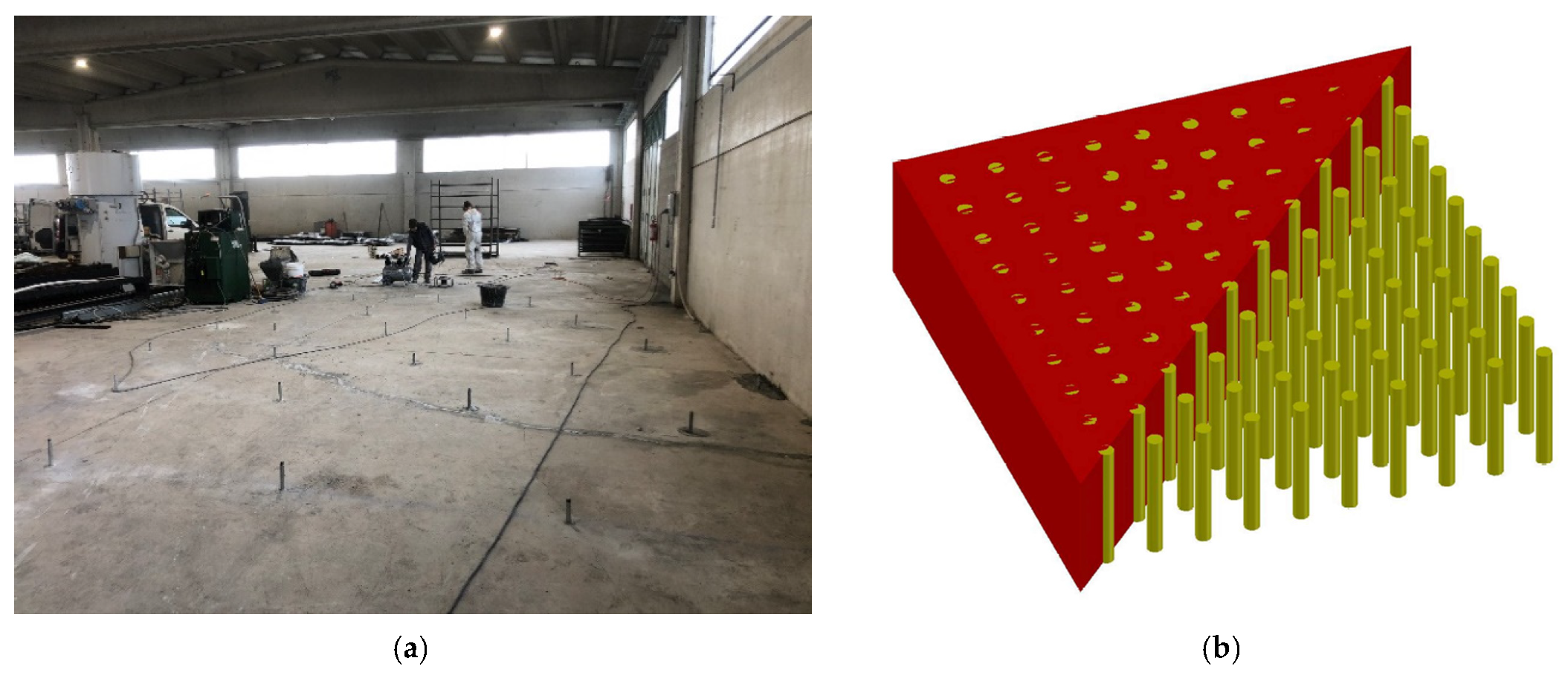
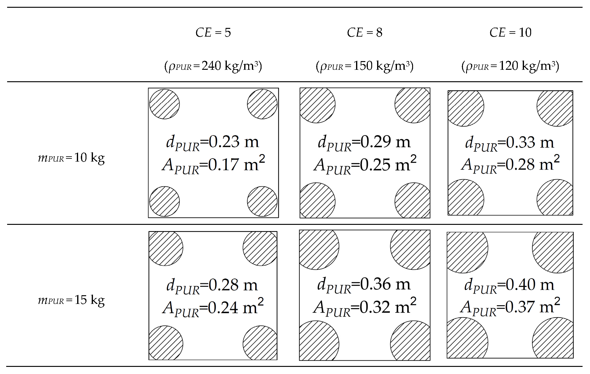
2. Soil Improvement Using Polyurethane

This section first describes the soil improvement technologies developed by Master Builders Solutions, based on the polyurethane injection. When injected inside the soil, polyurethane expands differently according to the soil type, having different final densities. Impact tests are therefore performed on polyurethane specimens realised with different densities, to determine a function for the elastic modulus and the damping coefficient varying with density.

2.1. Master Builders Solutions’ Technologies for Soil Improvement through Grouting

Among Master Builders Solutions’ technologies [42], injections of polyurethanes belonging to the “MasterRoc MP 35X” group are widespread for the improvement of foundation soils underneath existing buildings, and the group contemplates different polyurethane types, each suitable to a specific application. One of the most popular is the MasterRoc MP 355 [43], which is examined in our study.
There are different injection techniques, and among the most widespread is the technique related to resin injection to fill voids, cracks and cavities in soil/rock. The injection is preceded by making perforations of a diameter between 90 and 127 millimetres, where the injection pipes are inserted. The latter may be steel pipes of a small diameter (10–12 mm) or high-density polyethylene pipes PN25, inserted at different depths, according to the injection levels. At each injection level, the injections are separated through an obturator bag or mortar sheath. Pneumatic, electric or electro-hydraulic piston pumps are used (pressures up to 150–200 bar). The A- and B-components, whose mixture creates the polyurethane foam, have a high viscosity and need pressure to be pumped. The two components are therefore pumped into high-pressure pipes of a small diameter (an internal diameter of 6–10 mm), connected to the injection gun, where they are mixed through a static mixer. The pressure of the injection into the substrate is between 0 and 30 bar. Injections follow different schemes, according to the types of foundation and soil; in any case, they are realised in a bottom-up direction. In particular, this paper analyses the case of injections under foundation slabs. They are commonly realised on a grid spaced 0.5–1.5 m, injecting 10–20 kg of polyurethane mass per level, at 1–3 injection levels (the first injection level is usually immediately underneath the foundation surface, while the others are spaced 0.5 to 1 m in depth). Figure 1a shows an example of the application. Injected polyurethane expands differently according to the soil confinement, and the polyurethane expansion is quantified through a coefficient of expansion (CE), as shown in Equation (1).
CE = Vf/Vi = ρi/ρf
with Vi and Vf respectively being the initial and final volume of the polyurethane. By assuming a radial expansion of the material, the configuration of the injected layers is shown in Figure 1b, where the diameter of the expanded polyurethane will depend on CE. Thanks to the mass conservation, the volume ratio of Equation (1) corresponds to a density ratio of initial ρi versus final ρf.

3. Dynamic Characterisation of Polyurethane by Means of Laboratory Tests

Dynamic characterisation of a material means the determination of parameters that describe the material behaviour in dynamic conditions, and it is related to the wave propagation, affected by the wave propagation velocity and the damping coefficient. The wave velocity depends on the elastic modulus and the density; while the latter is easy to evaluate, the elastic modulus is determined with specific tests. In the following, an experimental program is performed for the evaluation of the stiffness and damping coefficient of polyurethane at different densities, preceded by the description of polyurethane sample preparation.

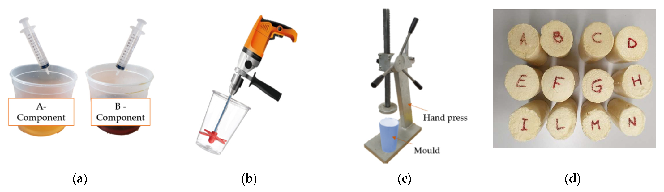
3.1. Sample Preparation
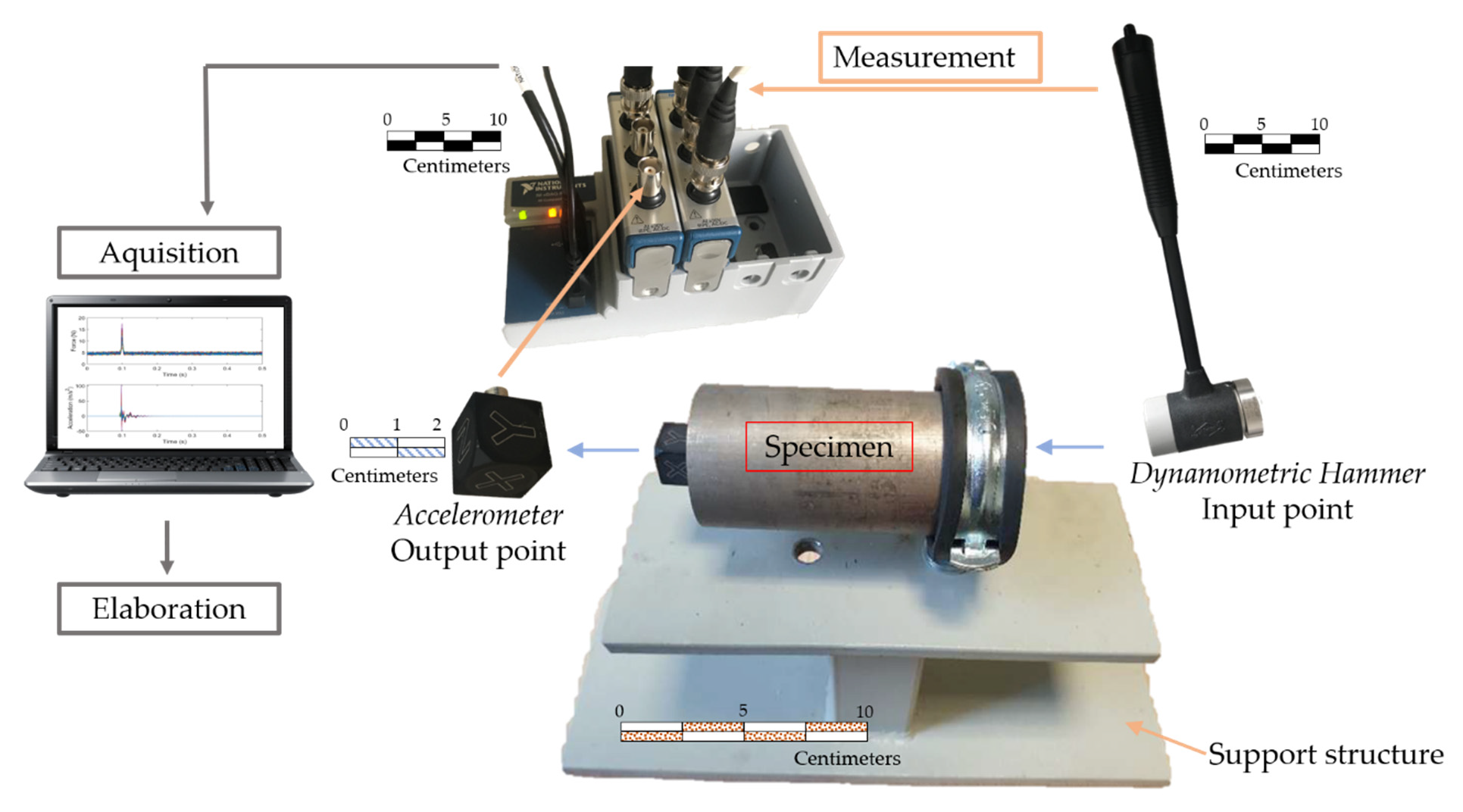
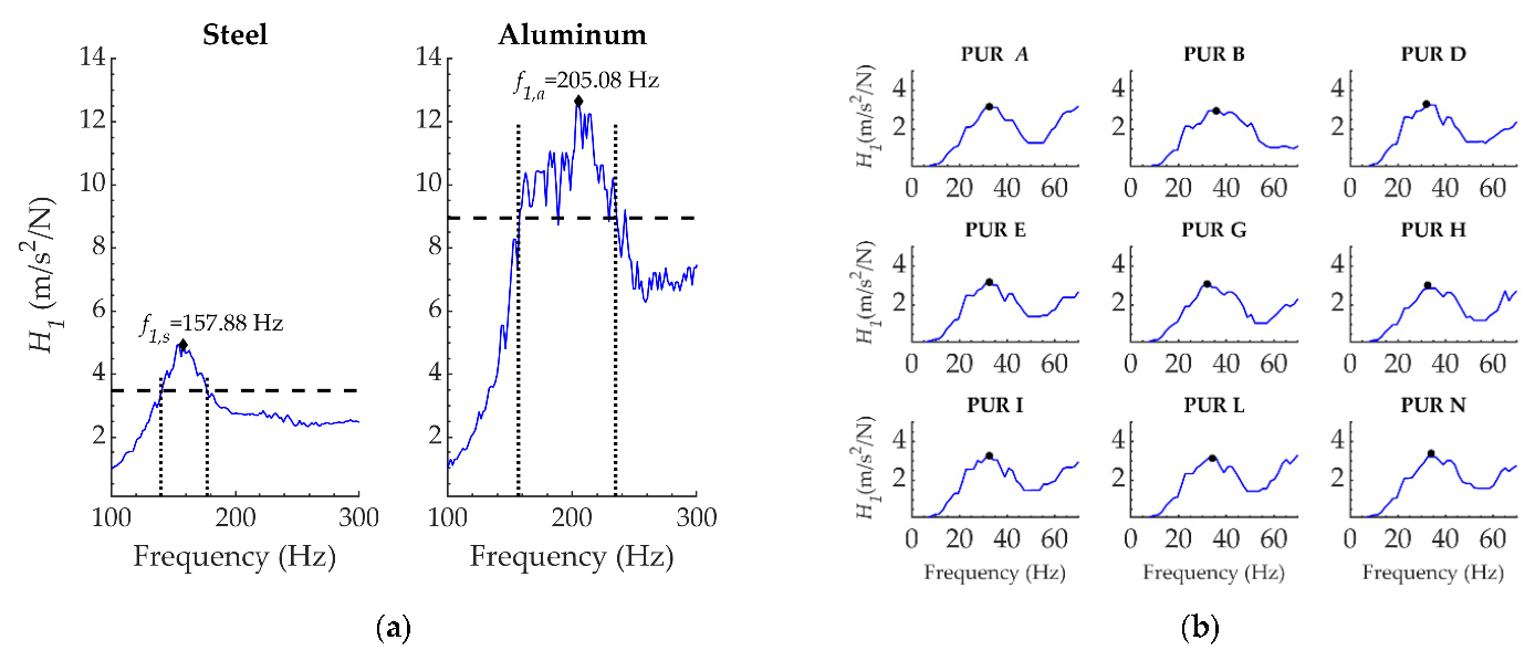
The main phases of polyurethane sample preparation are illustrated in Figure 2. Components A (polyol, density 1000 kg/m3) and B (isocyanate, density 1250 kg/m3) are mixed in a volumetric ratio of 1:1, as suggested by the Master Builders Solutions’ technical sheet [42], and 20 mL syringes are used for the volumetric control (Figure 2a). The two components are withdrawn separately, injected into a plastic cup and mixed using a propeller-equipped drill (Figure 2b) for an adequate mixing time to obtain a homogeneous foam (about 40 s, compatible with the setting time, after which the foam is not workable anymore). The mixture is then poured inside a cylindrical mould of height 0.10 m and diameter 0.045 m (volume 1.59 × 10⁻⁴ m3).
To study the dynamic properties of polyurethane at different densities, specimens are prepared at three expansion coefficients, CE = 6, 8 and 9. In free expansion, the foam has a CE equal to 9. It is possible to vary CE by forcing the foam to grow inside the mould’s volume (in other words, fixing the final volume, Vf) and changing only the initial volume, Vi (see Equation (1)). This is done thanks to the hand press shown in Figure 2c. Specifically, Vi,A = Vi,B = 15 mL for CE = 6, Vi,A = Vi,B = 11.25 mL for CE = 8 and Vi,A = Vi,B = 10 mL for CE = 9, with Vi,A and Vi,B being the initial volume of each component.
After having poured the mixture inside the mould, a few minutes are required for the foam setting and hardening process. Twelve specimens are realised (Figure 2d), and specimens are then weighted for the evaluation of the expansion coefficient in the aftermath.
The specimen weight, mA + B, depends on the densities and the initial volumes of A- and B-components, which allow to compute the initial volume of the polyurethane as:
Vi = 2 mA + B/(ρA + ρB)
from this relationship, Vi is computed for each specimen, and then the CEs are determined. CE values are shown in Table 1, and the specimen density is also reported.

3.2. Impact Tests

Cylindrical specimens with 4.5 cm in diameter and 10 cm in height are placed on the support structure shown in Figure 3, where they are bound with a ring. The impact test is performed by applying an impulsive force orthogonally to the bound base surface of the specimen, using the dynamometric hammer PCB 086D20. The dynamic response is recorded by means of a triaxial accelerometer PCB 356A16, glued to the free end. The test scheme is single input–single output (SISO). Tests are manually performed by an operator, and force magnitude is controlled by the hammer’s load cell.
Impact tests excite the specimens at frequency intervals, whose amplitude depends on the tip hammer’s material; in the excited interval, the natural frequencies are detected through the frequency response function, H1(f), computed by means of the Fourier transform of the measured force and acceleration, respectively Sf (in N) and Sa (in m/s2):
H 1 ( f ) = S f * · S a S f * · S f
with S f * being the complex conjugate of Sf; and H1 is therefore expressed in m/s2/N. In the following, the experimental results’ elaboration is described, for the evaluation of the elastic modulus and the damping coefficient of the specimens. In both cases, the first natural frequency identified, f1 (fundamental frequency), is considered, depending on the axial modal behaviour of the specimens for the test performed.
By schematising the one-degree-of-freedom system with a simple mass-spring-dashpot model, the fundamental frequency, f1, is equal to 1/(2π) k ^ / m , with m the specimen mass and k ^ a stiffness, taking into account not only the longitudinal stiffness of the sample (EA/L, with E the elastic modulus, A the cross-section area and L the length of the specimen) but also the ring binding the specimen; because of the impact, the boundary exerts an elastic reaction depending on a stiffness kstr. k ^ is therefore evaluated as the difference, EA/L−kstr; from f1 expression, the elastic modulus, E, is derived, simplified as:
E = ρ ( 2 π f L ) 2 C
where ρ is the material density (in kg/m3), f is the fundamental frequency (in Hz), while C is a calibration factor including both kstr and the physical and geometrical characteristics of the specimen in the examination (ρ, A and L). The length, L, is expressed in metres. To define an expression for C and calibrate the procedure of experimental data elaboration, the impact tests are initially conducted on steel and aluminium specimens, i.e., materials of known characteristics, of dimensions similar to those of polyurethane specimens.
From H1, it is possible to evaluate the damping coefficient associated to each system’s mode of vibration through the half-power bandwidth method, whose validity is proven for frequency response functions symmetric around the natural frequencies [36,44,45]. Specifically, for the evaluation of the damping coefficient associated to the first mode of vibration, after having detected the fundamental frequency, f1, the method consists of determining the two frequencies, fa and fb, where the value assumed by H1 is 1 / 2 H 1 (f1), and the damping coefficient is:
ξ ¯ = f b f a 2 f 1
where ξ ¯ refers to the system’s damping (support structure and specimen); even in this case, the experimental results of tests performed on specimens made up of material of known characteristics allow to calibrate the elaboration procedure, by reducing ξ ¯ for the evaluation of ξ , i.e., the material damping.

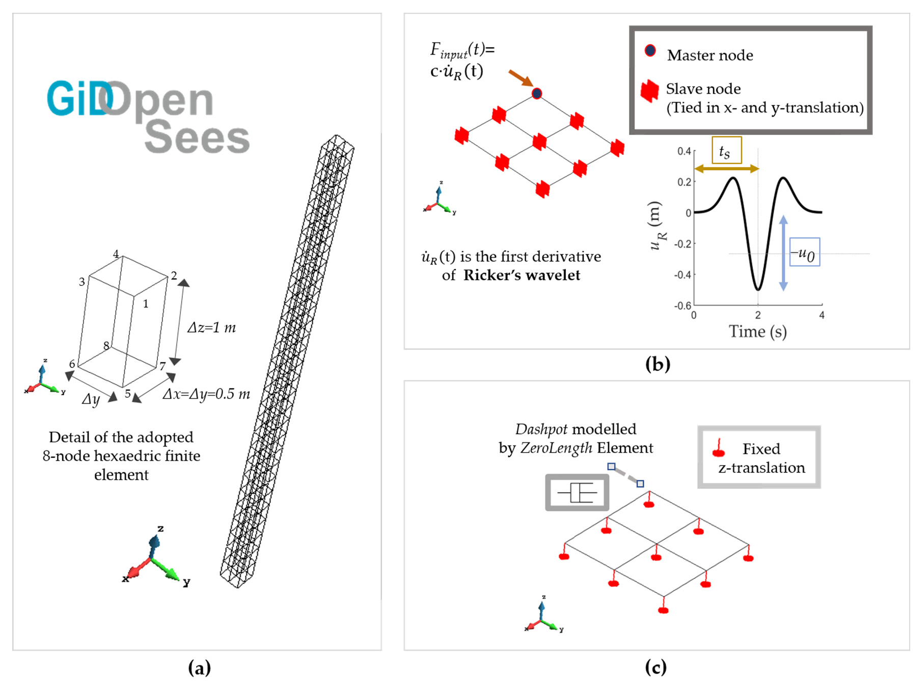
4. The Finite Element Numerical Model

Finite element (FE) numerical modelling was performed to evaluate the effect of polyurethane injections on the seismic response of cohesionless soils with different characteristics. OpenSees [37] was used, using the GiD graphic interface [38], and both of them are implemented in GiD + OpenSees [39]. A 30 m sand deposit with four relative densities, DR, was considered:
  • Loose sand (LS), with DR = 15–35%
  • Medium sand (MS), with DR = 35–65%
  • Medium-dense sand (MDS), with DR = 65–85%
  • Dense sand (DS), with DR = 85–100%
Polyurethane injections are assumed following the intervention schemes shown in Figure 1 for the improvement of soils under foundation slabs.

4.1. Model Description

The numerical analyses were performed on a soil column of base area Ab = 1 m2, H = 30 m high, discretised with 3D 9-node Standard Brick elements, each of them with a dimension 0.5 × 0.5 × 1 m3 (Figure 4a). The finite element dimensions respect the Lysmer’s relationship [46], so that Δz < vs/10 fmax (for the cases in exam, v s = 80 ÷ 250 m/s and fmax = 10 Hz). Two analysis phases are considered: a gravity analysis first, followed by a dynamic time-history analysis, in which a seismic event is simulated.
The ground motion was numerically introduced by applying a horizontal viscous force, F input ( t ) = c · u ˙ ( t ) , to a base end node. The force is proportional to the velocity time history, u ˙ ( t ) , of the ground motion, with the viscous coefficient c = ρ R · v s , r · A b [46,47]. ρ R and v s , r are the density and the shear wave velocity of the bedrock, respectively equal to 2500 t/m3 and 1000 m/s. A uniform shaking was simulated tying the force application node with the remaining base nodes, with master-slave conditions for x- and y-translations (Figure 4b). Periodic boundary conditions were also introduced by tying the nodes at the same vertical coordinate for x- and y-translation.
Ricker’s wavelet was chosen as ground motion [48]. This choice is common in the dynamic numerical analysis, because its amplitude may be easily scaled and the frequency controlled [49]. The displacement equation is:
u R = u 0 ( 2 u * -   1 ) e - u *
u * = [ π ( t   -   t s ) t p ]
where t p is the fundamental wavelet period, and t s is the time of the wavelet’s peak occurrence, corresponding to the maximum displacement u 0 ; in our case, t p   = 2 s, ts = 2 s and u 0 = 0.5 m. The velocity, u ˙ ( t ) , for the viscous input force is the first derivative of u R .
The bedrock (30 m below the surface) was introduced by bounding the z-translations of the column’s base nodes. A dashpot was modelled to absorb the reflecting boundary waves, taking into account the finite rigidity of the half-space below the bedrock [46]. For this purpose, two nodes at the same coordinates of the seismic input node are connected by a Zero-Length element of viscous uniaxial material, with damping coefficient c (Figure 4c).
The time step, · t , of the dynamic analysis was assumed equal to 0.005 s, fulfilling the Courant–Friedrich–Lewy relationship, v s   · t / · z     1 . 25 , discussed by LeVeque [50], for a more stable solution of the numerical analysis.
The Pressure-Dependent Multi-Yield (PDMY) model was used for the constitutive modelling of both the soil and the soil–polyurethane layers; in Section 4.2, a detailed description of the model is provided, to better explain how the composite material is numerically introduced.
Soil viscous damping was considered through Rayleigh’s frequency-dependent method [51] and the α and β coefficients; according to their values, the damping coefficient, ξ , can be varied with the frequency. In particular, α = (2 ξ ω1ω2)/(ω1 + ω2) and β = (2 ξ )/(ω1 + ω2), with ω1 and ω2, two target frequencies evaluated as ω1 = πvs/2H and ω2 = 5πvs/2H, i.e., the first and the third natural frequency of a theoretical amplification function for a visco-elastic deposit [52].
Since soil damping is known to be hysteretic and not dependent on the frequency, α and β are chosen so that ξ is constant in the frequency range of the soil modal response.

4.2. The Pressure-Dependent Multi-Yield Model (PDMY)

The PDMY is a hysteretic nonlinear model, based on the concept of multi-yield plasticity surfaces; it is suitable for modelling cohesionless materials, whose shear response depends on the confining pressure [53,54,55,56]. It is represented by a cone in the effective stress space. The model introduces the cyclic mobility, with emphasis placed on an accurate reproduction of accumulated shear strains in clean medium-dense cohesionless soils.
Some features of the model are summarised here, useful for our numerical application. Soil nonlinearity is introduced through a hyperbolic function for the octahedral stress–strain, τ - γ , relationship; at the reference pressure, p ref , its expression is:
τ = G ref · γ 1 + γ ( G ref τ f ref - 1 γ max )
where G ref and τ f ref are respectively the shear modulus and the failure octahedral shear stress, both of them in relation to p ref and expressed in kPa, and γ max is an octahedral strain where the hyperbole of Equation (7) becomes asymptotic. Note that Equation (7) implies a modulus decay curve, since a secant modulus is evaluable as τ / γ at each strain level.
The outer surface of the cone is defined by τ f ref , evaluated knowing the friction angle,   φ , and the reference pressure, p ref ,   as:
τ f ref = 2 2 sin φ 3   - sin φ p ref
A generic shear modulus, G , for the generic isotropic stress, p , is evaluated through an exponential distribution, of exponent d :
G = G ref ( p p ref ) d
The soil is modelled with the PDMY parameters suggested by the literature, experimentally calibrated [55], and the main values are reported in Table 2.
As described in Section 2.1, the polyurethane injections underneath the slab foundations involve drilling a grid and injections at several levels, each of them at about every metre of depth. For the case in examination, the grid spacing chosen is equal to 0.75 m, and four injections are therefore contained in the column cross-section (area 1 × 1 m2), at a distance of 0.75 m from one another and 0.125 m from the edge. Both two and three injection levels were chosen, resulting in injected surficial depths, h, equal to 2 and 3 metres. The polyurethane mass injected at each level, identified as m PUR , was set equal to 10 and 15 kg.
According to the soil confinement, the injected mass expands differently, occupying a volume quantified by the coefficient of expansion (CE). From Equation (1), assuming a radial expansion (see Figure 1b), the diameter of the rigid expanded polyurethane, d PUR (expressed in metres), is obtained, depending on the CE and m PUR (kg), through:
d PUR = 2 · CE · m PUR π · ρ i · 1 m
where   ρ i is the fluid density equal to 1200 kg/m3. Note that m PUR is considered as the mass injected every metre of depth, which is why the final volume introduced in the formula is 1 metre high. Since the relationship between CE and the soil confinement is not known for the soil under examination, CE is varied parametrically assuming CE = 5, 8 and 10, corresponding to rigid foam density ρPUR = 240, 150 and 120 kg/m3 (see Equation (1)).
The values of dPUR calculated through Equation (10) are reported in Figure 5, together with the area of the expanded polyurethane APUR contained in the 1 m2 column’s cross-section area.
The first metres of the soil column (h) represented in Figure 4a are therefore made up of a composite sand–polyurethane material, with polyurethane in different ρPUR and APUR. The PDMY model was also used for this material. To evaluate the parameters of the composite material, a homogenisation procedure is introduced; specifically, for density and damping, a linear homogenisation is considered, in the form:
ρ SP = ρ soil ( 1 - A PUR / A b ) + ρ PUR ( A PUR / A b )
ξ SP = ξ soil ( 1 - A PUR / A b ) + ξ PUR ( A PUR / A b )
As regards the stiffness, an appropriate procedure is shown calibrated through the results of resonant column tests performed on the composite material [35].

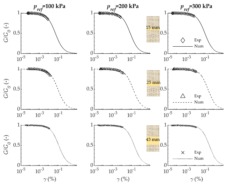
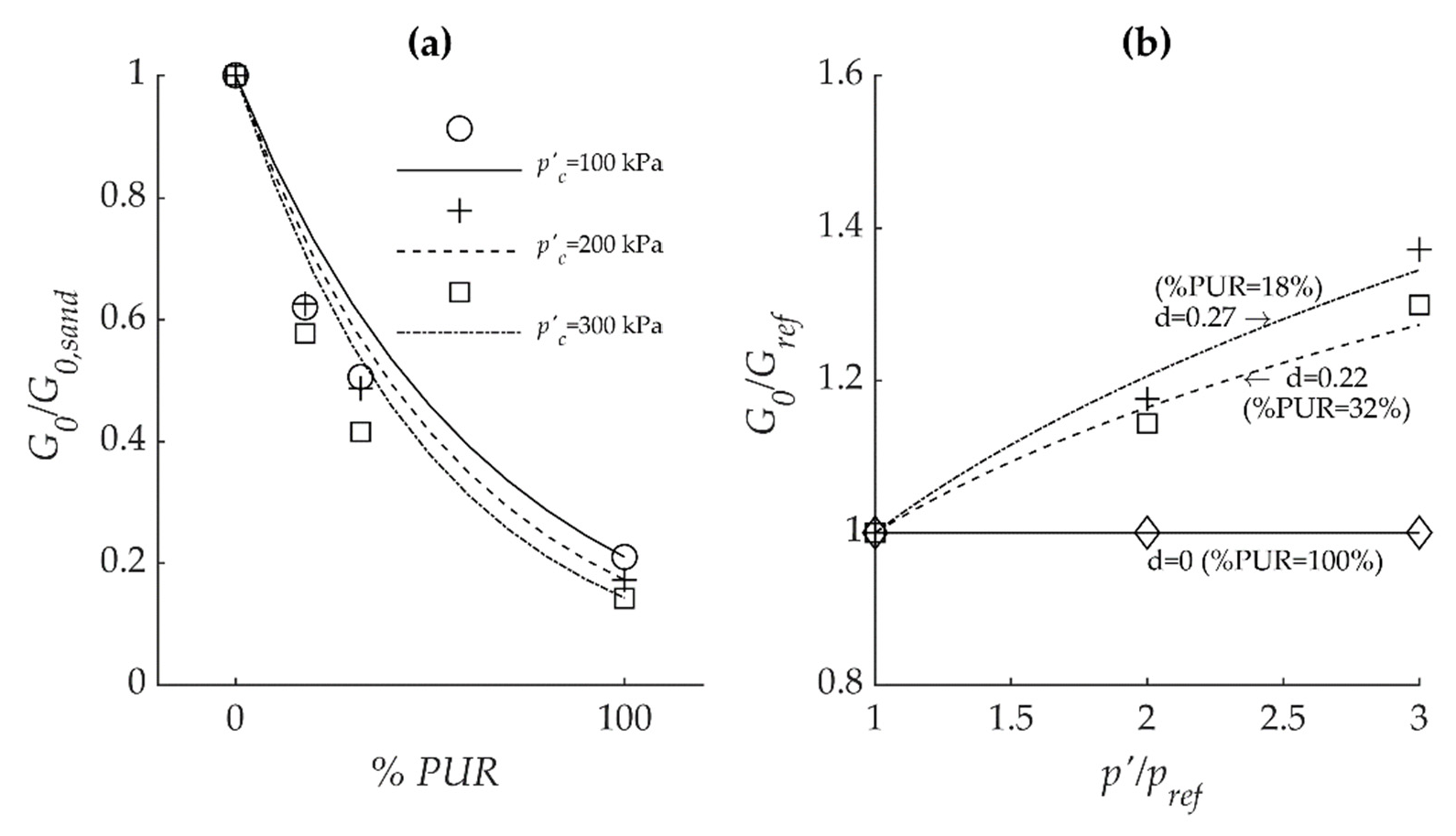
4.3. Calibration of the PDMY Constitutive Model for the Sand–Polyurethane Composite Material

Gatto et al. [35] performed resonant column tests on cylindrical specimens (diameter 7 cm, height 14 cm) of pure sand, pure polyurethane (density 90 kg/m3) and sand–polyurethane, with the polyurethane introduced at layers of 15, 25 and 45 mm thick, giving rise to different volumetric percentages of the polyurethane in the specimen.
Figure 6 illustrates the comparison between the experimental and the numerical shear modulus decay curves, G/G0, the latter obtained from Equation (7) for the PDMY material. The numerical curve is shown to well-interpret the experimental results.
A homogenisation expression was therefore derived for the evaluation of the small-strain stiffness of composite specimens, with the combination of the small-strain stiffness for pure sand (G0,sand) and pure polyurethane (G0,PUR) according to the polyurethane volumetric percentage (%PUR) in the specimen. This is necessary for the evaluation of the Gref associated to each case of Figure 5.
From the experimental results, the ratio G0/G0,sand was computed for each confining pressure (p’c = 100, 200 and 300 kPa), with G0 the small-strain shear modulus for the generic specimen. The experimental points G0/G0,sand-%PUR are plotted in Figure 7a, showing an exponential trend. The equation of a negative exponential distribution was derived for G0-%PUR, so that G0 is equal to G0,sand and G0,PUR respectively, for %PUR = 0 and %PUR = 100.
G 0 = G 0 , sand e ( ln G 0 , sand G 0 , PUR ) · % P U R / 100
Equation (12) is therefore a homogenisation formula, where G0, G0,sand and G0,PUR are expressed in MPa, and it is represented by the lines in Figure 7a, showing an acceptable comparison with the experimental points.
Note that G0 depends on the confining pressure through G0,sand, since G0,PUR is quite independent from the confining pressure [35]. For the numerical model, a homogenised shear modulus will be computed at a reference pressure; then, it is updated according to the specific model pressure through Equation (9).
The exponent d of Equation (9) is therefore derived for composite specimens, varying with the %PUR. G0 values experimentally obtained for the generic confining pressure, p’, were normalised with respect to the shear modulus evaluated at p’ref = 100 kPa, and the results are shown in Figure 7b, together with curves derived from Equation (9), with d values giving the best fit. d was observed to diminish by increasing the polyurethane volumetric percentage, going towards d = 0 for pure polyurethane specimen, whose stiffness is independent from the confining pressure. A linear expression describes the variation d (dimensionless) with the polyurethane percentage:
d = 0 . 33   -   0 . 0033 · ( % PUR / 100 )
Equations (12) and (13) were applied for the evaluation of the composite material parameters, according to the configuration.

5. Results

This section first shows the results of the dynamic characterisation of polyurethane specimens realised with different densities, followed by the results of the numerical analyses.

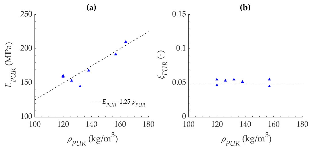
5.1. Elastic Modulus and Damping Coefficient for Polyurethane MP355 at Different Densities, Evaluated through Impact Tests

Figure 8a shows the frequency response functions, H1, evaluated through Equation (3) from the impact tests performed on steel and aluminium specimens: the fundamental frequencies are f1,s = 157.88 Hz and f1,al = 205.08 Hz. These results are used to define the kstr value, by [ ( E L -   4 π 2 ρ Lf 2 ) A ] . Knowing the elastic moduli for steel (Es = 210 GPa) and aluminium (Eal = 70 GPa), values of kstr,s = 3.34 × 10¹⁰ N/m and kstr,a = 1.11 × 10¹⁰ N/m were obtained. kstr is therefore not constant, by changing the material specimen, that which is constant is the ratio kstr/E. An empirical expression was derived for C (see Equation (4)), applicable knowing only the specimen geometry (area A and height L) and physical characteristics (density ρ ).
C = ( 1 - L A k str , s E s ) ( 2 - ρ ρ s ) 1 . 2
where ρs is the steel density. The elastic modulus predicted for the aluminium specimen is 69.9 MPa, comparable with its typical value.
The H1 computed from the experimental results of impact tests conducted on the polyurethane specimens are shown in Figure 8b; through Equations (4) and (14), the fundamental frequency and the density of each specimen (Table 1) allow us to evaluate the elastic modulus, EPUR.
For the damping coefficient evaluation, the half-power bandwidth method described in Section 3.2 was applied, and the results of tests performed on steel and aluminium specimens (Figure 8a) were used for the calibration. ξ ¯ evaluated through Equation (5) is equal to 0.12 for the steel specimen: since the common value of steel damping coefficient is 0.02, a reduction factor of 6 was introduced. With this reduction, the value predicted for aluminium is 0.03, considered acceptable. The method was therefore extended to all the polyurethane specimens.
Figure 9 illustrates the elastic modulus, E PUR (a), and the damping coefficient, ξ PUR (b), for polyurethane at different densities. The elastic modulus was observed to vary with the density according to a linear equation.
E PUR = 1.25   ρ PUR
with EPUR in MPa and ρPUR in kg/m3. On the other hand, pairs ξ PUR ρPUR stay on a horizontal line ( ξ PUR 0.05   ρ PUR ).

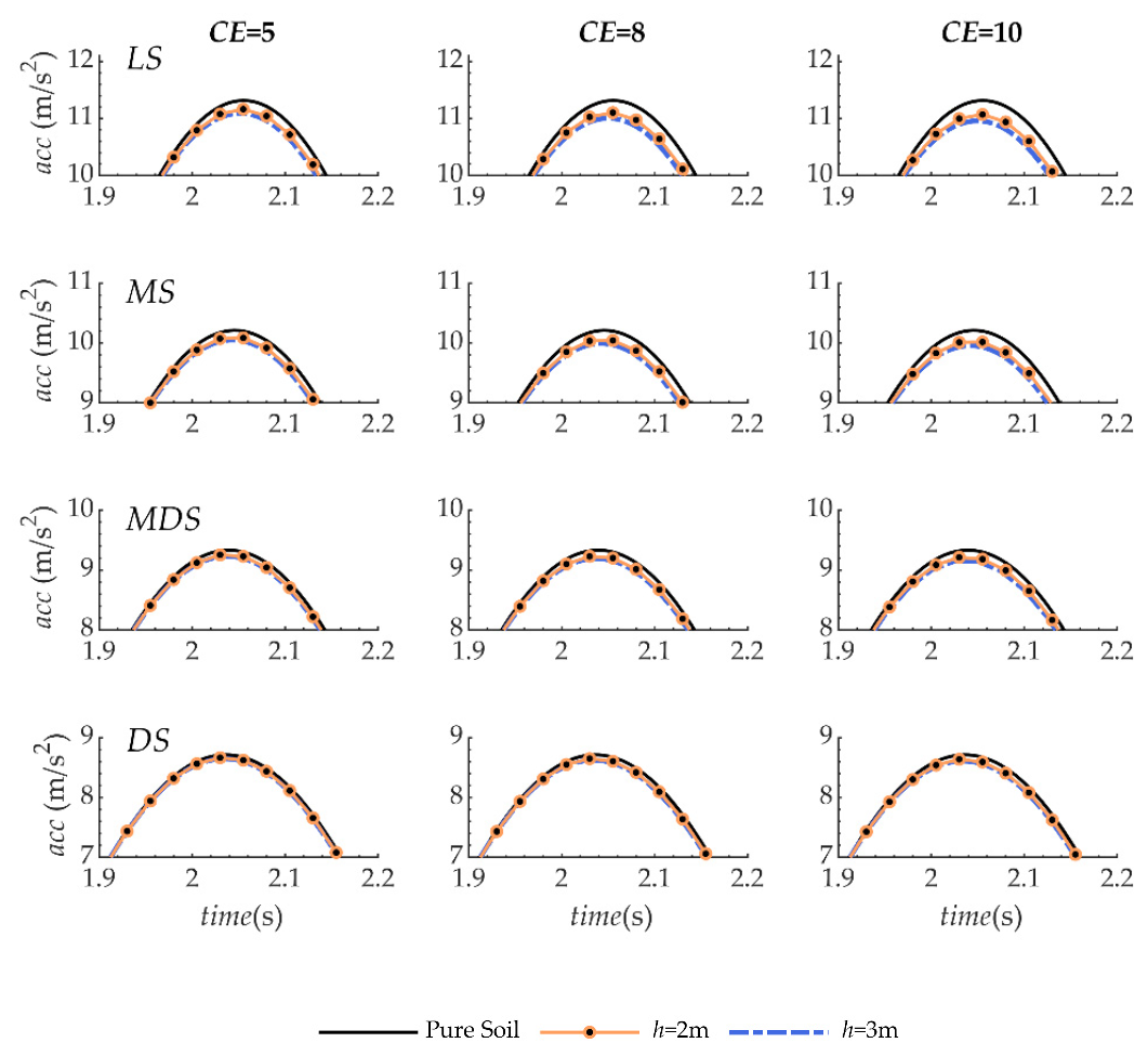
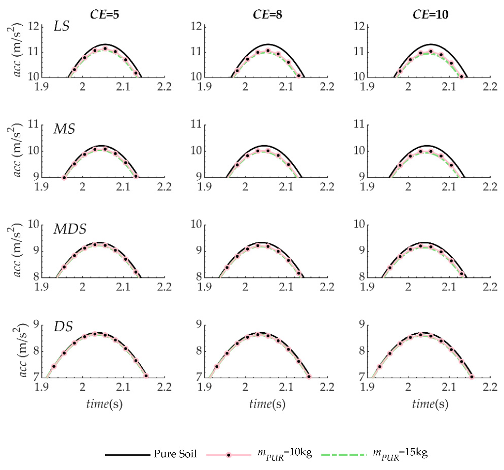
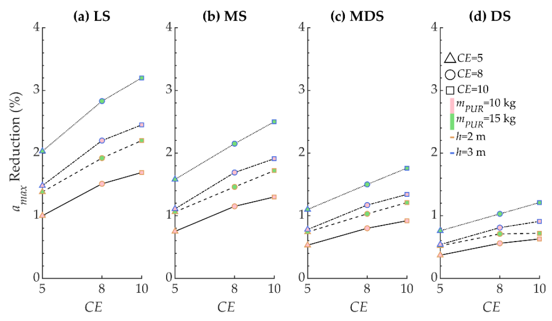
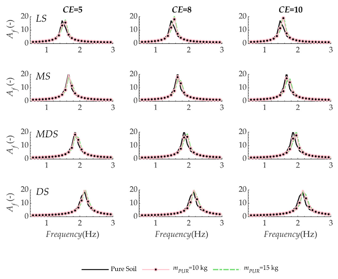
5.2. Seismic Response of Composite Material
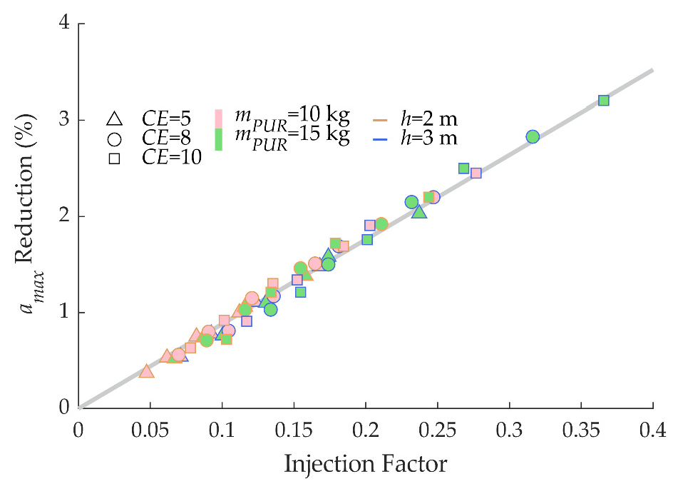
The cases considered in the numerical analyses have been reported in Figure 5, and each of them were used for both surficial injection depths, h = 2 and 3 m. The homogenised shear and bulk modulus for the injected layer was evaluated through Equation (12), while for density and damping, the linear homogenisation of Equation (11a,b) was used. For the cohesionless soils, the parameters at p’ref = 80 kPa were used (Table 2).
According to the polyurethane density of each case, the elastic modulus, EPUR, is evaluated through Equation (15), being EPUR = 300 MPa for CE = 5, EPUR = 187.5 MPa for CE = 8 and EPUR = 150 MPa for CE = 10. G 0 , PUR is then derived through the elastic theory ( G 0 , PUR = EPUR/2/(1 + νPUR)), with νPUR equal to 0.38.
Values of G for composite layers are reported in Table 3.
Figure 10 and Figure 11 show the horizontal x-accelerations recorded at the top of the model: the figures’ y-axes are restricted to the range that allows the appreciation of the differences among the cases. Both figures show the effects of polyurethane injections on the ground accelerations, with the three expansions assumed, in the cohesionless soil at four relative densities.
Particularly, Figure 10 shows that injecting 15 kg of polyurethane at 2 and 3 m injected depth gives rise to a reduction of maximum accelerations, growing with h. The best result was observed for loose sand and CE = 10, where the maximum accelerations are 11.31, 11.04 and 10.95 m/s2 respectively, for pure soil, and the injected soil with h = 2 m and h = 3 m. Minor acceleration reductions were observed for dense sand and CE = 5 (maximum accelerations are 8.71, 8.67 and 8.65 m/s2, for pure soil, h = 2 m and h = 3 m).
Figure 11 illustrates the accelerations of soils having h = 3 m, modified with 10 and 15 kg per injection level, together with accelerations of corresponding pure soils. Even in this case, reductions were greater injecting the loose sand with CE = 5; specifically, maximum accelerations were 11.15 and 11.09 m/s2 for mPUR = 10 kg and mPUR = 15 kg. It was observed that injecting a greater amount of polyurethane per level provides bigger reductions.
Both figures highlight that the injection interventions are more advantageous when soil is looser; with the same soil’s relative density, the reduction is greater when polyurethane expands more and its density is lower.
Results of Figure 10 and Figure 11 are summarised in Figure 12, by considering the ratio of the maximum accelerations of composite specimens to the maximum acceleration of the same soil type without intervention. Surficial acceleration reductions vary between 0.4% and 3.2%. In particular, better results are obtained by injecting, at a greater number of levels, much more polyurethane mass and causing polyurethane to expand more.
Amplification functions, Af, were also evaluated, to analyse the effects of polyurethane injection on the frequency response of the deposit; particularly, Af is computed by dividing the Fourier spectrum of surficial and base accelerations. Figure 13 shows Af of the models having h = 3 m, with mPUR equal to 10 and 15 kg. A slight increase of the fundamental frequency was observed in the composite models.

6. Discussion

The elastic modulus of polyurethane was shown to vary linearly with the polyurethane density, and this is in line with other literature results [32,57,58,59]. In particular, comparing with Horak et al.’s results [59], who derived the elastic moduli after compression tests, our results appear to overestimate the elastic modulus; however, dealing with a dynamic modulus, the overestimation is in agreement with the evidence in the literature regarding the ratio between the static and dynamic moduli [60].
The numerical results provide evidence that the accelerations are reduced in relation to the polyurethane volumetric percentage, and this is in agreement with previous findings [35]. In terms of reduction, better results were found when polyurethane expands more and it results in a less dense foam; moreover, the looser the soil is where the polyurethane is injected, the more the accelerations were reduced. Other examples of geotechnical seismic isolation methods have shown that low-density materials have good effects in acceleration reductions [20,22]. Our results confirmed this evidence, adding that the reduction is proportional to the shear moduli ratio of polyurethane–soil, more in general.
With a view to summarise the results of Figure 12, a factor is introduced, taking into account the polyurethane shear modulus and volumetric percentage, as well as the shear modulus of the soil ( G soil ). For the polyurethane, both the modulus and its percentage depend on the injected mass, m PUR , the number of injections, n inj , and the expansion, CE . We named this factor the injection factor, IF, and it is equal to:
I F = G PUR   · A PUR · h G soil   · A · H · CE = F k n inj · m PUR · h G soil   · A · H · CE  
where F k is a factor taking into account the polyurethane elastic modulus–density relation, h is the injected soil depth (expressed in metre), H (in m) and A (in m2) are the total height and the cross area of the homogeneous soil deposit and m PUR is expressed in kg. Each case numerically analysed can be described by a value of IF. By representing the acceleration reduction with the injection factor, Figure 14 was obtained.
Results are interpreted by a linear function, showing the direct proportionality between the acceleration reduction, the injected mass and its expansion, inverse proportionality with the soil shear modulus, meaning that better results are expected in less stiff soil.
Equation (16) can be used for the preliminary design of an intervention of polyurethane injection; according to the desired acceleration reduction, necessary for the structure’s protection, the number of injections in the intervention area, the number of injection levels (i.e., the injected depth) and the injected mass per level can be chosen.
However, the expansion coefficient is not a variable that can be set arbitrarily by the user, it depends on the soil itself (in terms of type and confinement). A relationship CEGsoil needs to be derived.
Note that numerical analyses for the investigation about the use of this technique on a generic soil must be preceded by an experimental campaign on pure soil, pure polyurethane and composite soil–polyurethane in order to define the appropriate homogenisation expression for the soil to be treated.

7. Conclusions

The effect of polyurethane injections on the surficial seismic response of cohesionless soils, having different relative densities, has been investigated through FE numerical analyses. Such interventions through polyurethane injection are in use for soil improvement and are widely applied under the foundations of existing buildings. By considering the fact that polyurethane expands differently according to the soil confinement, different expansion coefficients have been considered. Results have shown that the surficial accelerations were reduced proportionally to the shear moduli ratio of polyurethane and soil, as well as the polyurethane percentage in the volume intervention. The injection factor was introduced for a preliminary quantification of the acceleration reduction, depending on soil stiffness, number of injections, number of injection levels and mass injected per level, as well as the expansion coefficient of the polyurethane. However, the expansion coefficient is dependent on the soil and a correlation with the soil confinement should be found. Further investigation will be conducted in this direction, together with the method application of a real case, preceded by experimental tests for the homogenisation characteristics of the soil–polyurethane composite material.

Author Contributions

Conceptualization, L.M.; Data curation, D.G.; Formal analysis, M.P.A.G.; Funding acquisition, F.C. and L.M.; Investigation, D.G.; Methodology, L.M.; Writing—original draft, M.P.A.G.; Writing—review & editing, V.L., F.C. and L.M. All authors have read and agreed to the published version of the manuscript.

Funding

This research work was partially funded by the company Master Builders Solutions Italia SpA, part of MBCC group, through the research contract entitled “Studio e realizzazione di innovativi sistemi di trattamento dei terreni, basati sull’impiego di resine poliuretaniche, per l’attenuazione sismica dei terreni” stipulated with the Department of Engineering & Architecture - University of Parma and partially funded by the MIUR (Ministry of Education, Universities and Research [Italy]) through the project entitled “eWAS: an early WArning System for urban-heritage”.

Institutional Review Board Statement

Not applicable.

Informed Consent Statement

Not applicable.

Data Availability Statement

Not applicable.

Acknowledgments

The Authors would like to thank the company Bequadro S.r.l. (https://bequadro.eu/, accessed on 29 April 2021) for the photo shown in Figure 1a, regarding their application of the polyurethane injection and the authors acknowledge financial support from the MIUR (Ministry of Education, Universities and Research [Italy]) through the project entitled “eWAS: an early WArning System for urban-heritage” (Project code: ARS01_00926/CUP J66C18000390005), financed with the PNR 2015-2020 (National Research Program). We authorize the MIUR to reproduce and distribute reprints for Governmental purposes, notwithstanding any copyright notations thereon. Any opinions, findings, and conclusions or recommendations expressed in this material are those of the authors and do not necessarily reflect the views of the MIUR.

Conflicts of Interest

The authors declare no conflict of interest.

References

  1. Furtado, A.; Vila-Pouca, N.; Varum, H.; Arêde, A. Study of the Seismic Response on the Infill Masonry Walls of a 15-Storey Reinforced Concrete Structure in Nepal. Buildings 2019, 9, 39. [Google Scholar] [CrossRef] [Green Version]
  2. Gautam, D.; Rodrigues, H. Impacts and Insights of Gorkha Earthquake in Nepal; Elsevier: Amsterdam, The Netherlands, 2018. [Google Scholar]
  3. Anelli, A.; Santa-Cruz, S.; Vona, M.; Tarque, N.; Laterza, M. A proactive and resilient seismic risk mitigation strategy for existing school buildings. Struct. Infrastruct. Eng. 2019, 15, 137–151. [Google Scholar] [CrossRef]
  4. Han, Z.; Lu, X.; Hörhager, E.I.; Yan, J. The effects of trust in government on earthquake survivors’ risk perception and preparedness in China. Nat. Hazards 2017, 86, 437–452. [Google Scholar] [CrossRef]
  5. Jones, S.; Oven, K.J.; Wisner, B. A comparison of the governance landscape of earthquake risk reduction in Nepal and the Indian State of Bihar. Int. J. Disaster Risk Reduct. 2016, 15, 29–42. [Google Scholar] [CrossRef] [Green Version]
  6. Castelli, F.; Lentini, V.; Grasso, S. Recent developments for the seismic risk assessment. Bull. Earthq. Eng. 2017, 15, 5093–5117. [Google Scholar] [CrossRef]
  7. Fardis, M.N.; Panagiotakos, T.B. Seismic Design And Response Of Bare And Masonry-Infilled Reinforced Concrete Buildings. Part Ii: Infilled Structures. J. Earthq. Eng. 1997, 1, 475–503. [Google Scholar] [CrossRef]
  8. Barbagallo, F.; Bosco, M.; Marino, E.M.; Rossi, P.P.; Stramondo, P.R. A multi-performance design method for seismic upgrading of existing RC frames by BRBs. Earthq. Eng. Struct. Dyn. 2017, 46, 1099–1119. [Google Scholar] [CrossRef]
  9. Barbagallo, F.; Bosco, M.; Marino, E.M.; Rossi, P.P. Seismic retrofitting of braced frame buildings by RC rocking walls and viscous dampers. Earthq. Eng. Struct. Dyn. 2018, 47, 2682–2707. [Google Scholar] [CrossRef]
  10. Pantò, B.; Rossi, P.P. A new macromodel for the assessment of the seismic response of infilled RC frames. Earthq. Eng. Struct. Dyn. 2019, 48, 792–817. [Google Scholar] [CrossRef]
  11. Barbagallo, F.; Bosco, M.; Marino, E.M.; Rossi, P.P. Variable vs. invariable elastic response spectrum shapes: Impact on the mean annual frequency of exceedance of limit states. Eng. Struct. 2020, 214, 110620. [Google Scholar] [CrossRef]
  12. Romis, F.; Caprili, S.; Salvatore, W.; Ferreira, T.M.; Lourenço, P.B. An Improved Seismic Vulnerability Assessment Approach for Historical Urban Centres: The Case Study of Campi Alto di Norcia, Italy. Appl. Sci. 2021, 11, 849. [Google Scholar] [CrossRef]
  13. Ghasemi, S.; Nezamabadi, M.F.; Moghadam, A.S.; Hosseini, M. Optimization of relative-span ratio in rocking steel braced dual-frames. Bull. Earthq. Eng. 2021, 19, 805–829. [Google Scholar] [CrossRef]
  14. Rodrigues, H.; Arêde, A.; Furtado, A.; Rocha, P. Seismic Rehabilitation of RC Columns Under Biaxial Loading: An Experimental Characterization. Structures 2015, 3, 43–56. [Google Scholar] [CrossRef]
  15. Furtado, A.; Rodrigues, H.; Varum, H.; Arêde, A. Mainshock-aftershock damage assessment of infilled RC structures. Eng. Struct. 2018, 175, 645–660. [Google Scholar] [CrossRef]
  16. Hermanns, L.; Fraile, A.; Alarcón, E.; Álvarez, R. Performance of buildings with masonry infill walls during the 2011 Lorca earthquake. Bull. Earthq. Eng. 2014, 12, 1977–1997. [Google Scholar] [CrossRef] [Green Version]
  17. Tsang, H.-H. Seismic isolation by rubber–soil mixtures for developing countries. Earthq. Eng. Struct. Dyn. 2008, 37, 283–303. [Google Scholar] [CrossRef]
  18. Tsang, H.-H.; Lo, S.H.; Xu, X.; Neaz Sheikh, M. Seismic isolation for low-to-medium-rise buildings using granulated rubber-soil mixtures: Numerical study. Earthq. Eng. Struct. Dyn. 2012, 41, 2009–2024. [Google Scholar] [CrossRef]
  19. Abate, G.; Gatto, M.; Massimino, M.R.; Pitilakis, D. Large scale soil-foundation-structure model in greece: Dynamic tests vs fem simulation. In Proceedings of the 6th International Conference on Computational Methods in Structural Dynamics and Earthquake Engineering (COMPDYN 2017), Rhodes Island, Greece, 15–17 June 2017; pp. 1347–1359. [Google Scholar] [CrossRef] [Green Version]
  20. Pitilakis, K.; Karapetrou, S.; Tsagdi, K. Numerical investigation of the seismic response of RC buildings on soil replaced with rubber–sand mixtures. Soil Dyn. Earthq. Eng. 2015, 79, 237–252. [Google Scholar] [CrossRef]
  21. Argyroudis, S.; Palaiochorinou, A.; Mitoulis, S.; Pitilakis, D. Use of rubberised backfills for improving the seismic response of integral abutment bridges. Bull. Earthq. Eng. 2016, 14, 3573–3590. [Google Scholar] [CrossRef] [Green Version]
  22. Tsiavos, A.; Alexander, N.A.; Diambra, A.; Ibraim, E.; Vardanega, P.J.; Gonzalez-Buelga, A.; Sextos, A. A sand-rubber deformable granular layer as a low-cost seismic isolation strategy in developing countries: Experimental investigation. Soil Dyn. Earthq. Eng. 2019, 125, 105731. [Google Scholar] [CrossRef]
  23. Tsang, H.; Tran, D.; Hung, W.; Pitilakis, K.; Gad, E.F. Performance of geotechnical seismic isolation system using rubber-soil mixtures in centrifuge testing. Earthq. Eng. Struct. Dyn. 2020, 50, 1271–1289. [Google Scholar] [CrossRef]
  24. Forcellini, D. Assessment of Geotechnical Seismic Isolation (GSI) as a Mitigation Technique for Seismic Hazard Events. Geosciences 2020, 10, 222. [Google Scholar] [CrossRef]
  25. Bathurst, R.J.; Zarnani, S.; Gaskin, A. Shaking table testing of geofoam seismic buffers. Soil Dyn. Earthq. Eng. 2007, 27, 324–332. [Google Scholar] [CrossRef]
  26. Azinović, B.; Koren, D.; Kilar, V. The seismic response of low-energy buildings founded on a thermal insulation layer—A parametric study. Eng. Struct. 2014, 81, 398–411. [Google Scholar] [CrossRef]
  27. Karatzia, X.A.; Mylonakis, G.E. Geotechnical seismic isolation using EPS geofoam around piles. In Proceedings of the 6th International Conference on Computational Methods in Structural Dynamics and Earthquake Engineering (COMPDYN 2017), Rhodes Island, Greece, 15–17 June 2017; pp. 1042–1057. [Google Scholar] [CrossRef] [Green Version]
  28. Yegian, M.K.; Kadakal, U. Foundation isolation for seismic protection using a smooth synthetic liner. J. Geotech. Geoenviron. Eng. 2004, 130, 1121–1130. [Google Scholar] [CrossRef]
  29. Yegian, M.K.; Catan, M. Soil Isolation for Seismic Protection Using a Smooth Synthetic Liner. J. Geotech. Geoenviron. Eng. 2004, 130, 1131–1139. [Google Scholar] [CrossRef]
  30. Banović, I.; Radnić, J.; Grgić, N. Geotechnical Seismic Isolation System Based on Sliding Mechanism Using Stone Pebble Layer: Shake-Table Experiments. Shock Vib. 2019, 2019, 1–26. [Google Scholar] [CrossRef]
  31. Cavallaro, A.; Castelli, F.; Ferraro, A.; Grasso, S.; Lentini, V. Site response analysis for the seismic improvement of a historical and monumental building: The case study of Augusta Hangar. Bull. Eng. Geol. Environ. 2018, 77, 1217–1248. [Google Scholar] [CrossRef]
  32. Saint-Michel, F.; Chazeau, L.; Cavaillé, J.-Y.; Chabert, E. Mechanical properties of high density polyurethane foams: I. Effect of the density. Compos. Sci. Technol. 2006, 66, 2700–2708. [Google Scholar] [CrossRef]
  33. Montrasio, L.; Gatto, M.P.A. Experimental Analyses on Cellular Polymers for Geotechnical Applications. Procedia Eng. 2016, 158, 272–277. [Google Scholar] [CrossRef] [Green Version]
  34. Montrasio, L.; Gatto, M.P.A. Experimental analyses on cellular polymers in different forms for geotechnical applications. In Proceedings of the ICSMGE 2017—19th International Conference on Soil Mechanics and Geotechnical Engineering, Seoul, Korea, 17–27 September 2017; pp. 1063–1066. [Google Scholar]
  35. Gatto, M.P.A.; Montrasio, L.; Tsinaris, A.; Pitilakis, D.; Anastasiadis, A. The dynamic behaviour of polyurethane foams in geotechnical conditions. In Proceedings of the 7th International Conference on Earthquake Geotechnical Engineering, Rome, Italy, 17–20 June 2019; pp. 2566–2573. [Google Scholar]
  36. Gatto, M.P.A.; Montrasio, L.; Berardengo, M.; Vanali, M. Experimental Analysis of the Effects of a Polyurethane Foam on Geotechnical Seismic Isolation. J. Earthq. Eng. 2020, 1–22. [Google Scholar] [CrossRef]
  37. Mazzoni, S.; McKenna, F.; Scott, M.H.; Fenves, G.L. OpenSees Command Language Manual; Pacific Earthquake Engineering Research (PEER) Center: Berkeley, CA, USA, 2006. [Google Scholar]
  38. Coll, A.; Ribó, R.; Pasenau, M.; Escolano, E.; Perez, J.S.; Melendo, A.; Monros, A.; Gárate, J. GiD v.14 Reference Manual. 2018. Available online: www.gidhome.com (accessed on 25 May 2020).
  39. Papanikolaou, V.K.; Kartalis-Kaounis, T.; Protopapadakis, V.K.; Papadopoulos, T. GiD+OpenSees Interface: An Integrated Finite Element Analysis Platform; Lab of R/C and Masonry Structures, Aristotle University of Thessaloniki: Thessaloniki, Greece, 2017. [Google Scholar]
  40. Castelli, F.; Cavallaro, A.; Ferraro, A.; Grasso, S.; Lentini, V.; Massimino, M.R. Static and dynamic properties of soils in Catania (Italy). Ann. Geophys. 2018, 61, SE221. [Google Scholar] [CrossRef]
  41. Ciancimino, A.; Lanzo, G.; Alleanza, G.A.; Amoroso, S.; Bardotti, R.; Biondi, G.; Cascone, E.; Castelli, F.; Di Giulio, A.; D’onofrio, A.; et al. Dynamic characterization of fine-grained soils in Central Italy by laboratory testing. Bull. Earth. Eng. 2020, 18, 5503–5531. [Google Scholar] [CrossRef]
  42. Master Builders Solutions. Available online: https://www.master-builders-solutions.com/it-it (accessed on 15 January 2021).
  43. MasterRoc MP 355—Master Builders Solutions. Available online: https://assets.master-builders-solutions.com/it-it/tds-masterroc-mp355-it.pdf (accessed on 15 January 2021).
  44. Brandt, A.; Berardengo, M.; Manzoni, S.; Cigada, A. Scaling of mode shapes from operational modal analysis using harmonic forces. J. Sound Vib. 2017, 407, 128–143. [Google Scholar] [CrossRef]
  45. Brandt, A.; Berardengo, M.; Manzoni, S.; Vanali, M.; Cigada, A. Global scaling of operational modal analysis modes with the OMAH method. Mech. Syst. Signal Process. 2019, 117, 52–64. [Google Scholar] [CrossRef] [Green Version]
  46. Lysmer, J.; Kuhlemeyer, R.L. Finite Dynamic Model for Infinite Media. J. Eng. Mech. Div. 1969, 95, 859–877. [Google Scholar] [CrossRef]
  47. Joyner, W.B.; Chen, A.T.F. Calculation of nonlinear ground response in earthquakes. Bull. Seismol. Soc. Am. 1975, 65(5), 1315–1336. [Google Scholar]
  48. Ricker, N. Transient Waves in Visco-Elastic Media; Elsevier Science: Amsterdam, The Netherlands, 1977. [Google Scholar]
  49. Loli, M.; Knappett, J.A.; Anastasopoulos, I.; Brown, M.J. Use of Ricker motions as an alternative to pushover testing. Int. J. Phys. Model. Geotech. 2015, 15, 44–55. [Google Scholar] [CrossRef] [Green Version]
  50. LeVeque, R.J. Finite Difference Methods for Ordinary and Partial Differential Equations—Steady-State and Time-Dependent Problems; SIAM: Philadelphia, PA, USA, 2007. [Google Scholar]
  51. Chopra, A.K. Dynamics of Structures: Theory and Applications to Earthquake Engineering; Prentice Hall: Upper Saddle River, NJ, USA, 2011. [Google Scholar]
  52. Kramer, S.L. Geotechnical Earthquake Engineering; Prentice Hall: Upper Saddle River, NJ, USA, 1996. [Google Scholar]
  53. Parra, E. Numerical Modeling of Liquefaction and Lateral Ground Deformation Including Cyclic Mobility and Dilation Response in Soil Systems; Rensselaer Polytechnic Institute: Troy, NY, USA, 1996. [Google Scholar]
  54. Yang, Z.; Elgamal, A.; Parra, E. Computational Model for Cyclic Mobility and Associated Shear Deformation. J. Geotech. Geoenviron.Eng. 2003, 129, 1119–1127. [Google Scholar] [CrossRef]
  55. Elgamal, A.; Yang, Z.; Parra, E.; Ragheb, A. Modeling of cyclic mobility in saturated cohesionless soils. Int. J. Plast. 2003, 19, 883–905. [Google Scholar] [CrossRef]
  56. Dafalias, Y.F.; Manzari, M.T. Simple Plasticity Sand Model Accounting for Fabric Change Effects. J. Eng. Mech. ASCE 2004, 130. [Google Scholar] [CrossRef]
  57. Patel, P.S.; Shepherd, D.E.; Hukins, D.W. Compressive properties of commercially available polyurethane foams as mechanical models for osteoporotic human cancellous bone. BMC Musculoskelet. Disord. 2008, 9, 137. [Google Scholar] [CrossRef] [PubMed] [Green Version]
  58. Qiu, D.; He, Y.; Yu, Z. Investigation on compression mechanical properties of rigid polyurethane foam treated under random vibration condition: An experimental and numerical simulation study. Materials 2019, 12, 3385. [Google Scholar] [CrossRef] [PubMed] [Green Version]
  59. Horak, Z.; Dvorak, K.; Zarybnicka, L.; Vojackova, H.; Dvorakova, J.; Vilimek, M. Experimental measurements of mechanical properties of pur foam used for testing medical devices and instruments depending on temperature, density and strain rate. Materials 2020, 13, 4560. [Google Scholar] [CrossRef]
  60. Brotons, V.; Tomás, R.; Ivorra, S.; Grediaga, A.; Martínez, J.M.; Benavente, D.; Heras, M.G. Improved correlation between the static and dynamic elastic modulus of different types of rocks. Mater. Struct. 2015, 49, 3021–3037. [Google Scholar] [CrossRef] [Green Version]
Figure 1. Polyurethane injection scheme underneath foundation slabs: (a) Application example realised by Bequadro S.r.l., and (b) schematisation of polyurethane injections as cylinders (green) in the soil matrix (red).
Geosciences 11 00201 g001
Figure 2. Sample preparation: (a) Sampling of the two components with syringes (Volume ratio 1:1), (b) injection of both components into a plastic cup being mixed through a propeller-equipped drill, (c) outpour of the mixed foam inside a mould, closed by a hand press, and (d) specimens for tests.
Geosciences 11 00201 g002
Figure 3. Scheme of the impact test performed, with details of the instruments used.
Geosciences 11 00201 g003
Figure 4. FE numerical modelling: (a) 3D model and finite element adopted, (b) input application at an end node of the base, with master-slave node for uniform excitation introduction, and (c) modelling of a viscous-elastic bedrock.
Geosciences 11 00201 g004
Figure 5. Summary of the injection cases analysed. The polyurethane diameter and area are shown, corresponding to each considered combination injected mass per level, m PUR —expansion coefficients CE.
Geosciences 11 00201 g005
Figure 6. Numerical (Num) vs. experimental (Exp) comparison of the shear modulus decay for composite sand–polyurethane samples at three thicknesses (15, 25 and 45 mm) and for three confining pressures.
Geosciences 11 00201 g006
Figure 7. Homogenisation procedure of the small-strain parameters for the composite specimens. (a) Experimental (points) vs. analytical (lines) G0/G0,sand varying with the polyurethane volumetric percentage. (b) Calibration of d exponent for shear modulus variation with the isotropic stress.
Geosciences 11 00201 g007
Figure 8. Frequency response functions, H1, for (a) steel and aluminium specimens and (b) polyurethane specimens at different densities. In both figures, the marker shows the fundamental frequencies; in Figure (a), the application of the half-power bandwidth method for the damping evaluation is also illustrated.
Geosciences 11 00201 g008
Figure 9. Parameters obtained from the elaboration of impact test results. Variation with polyurethane density of (a) the elastic modulus and (b) the damping coefficient.
Geosciences 11 00201 g009
Figure 10. Time-history accelerations recorded on numerical models of pure cohesionless soil at different relative densities and on “modified” cohesionless soil: evidence of the effects of the thickness of the modified layer (mPUR = 15 kg injected per level).
Geosciences 11 00201 g010
Figure 11. Time-history accelerations recorded on numerical models of pure cohesionless soil at different relative densities and on “modified” cohesionless soil: evidence of the effects of the mass injected per level (h = 3 m).
Geosciences 11 00201 g011
Figure 12. Summary of the acceleration reductions.
Geosciences 11 00201 g012
Figure 13. Amplification functions for h = 3 m and mPUR = 10 and 15 kg.
Geosciences 11 00201 g013
Figure 14. Reduction of surficial accelerations in relation to the injection factor, representative of the number of injections, mass of injected polyurethane, depth of injected soil, as well as the soil stiffness.
Geosciences 11 00201 g014
Table 1. Summary of the polyurethane specimens with related properties.
SpecimenInitial CEMass, mA + B
(g)
Vi
(mL)
Final CEDensity, ρPUR
(kg/m3)
A625227.16157
B626236.88164
C624217.45151
D625227.16157
E821198.52132
F819179.41120
G822208.13138
H822208.13138
I920188.94126
L919179.41120
M918169.94113
N919179.41120
Table 2. Density, ρ, elastic properties (shear and bulk moduli, Gref and Bref) at a reference confining pressure (80 kPa) and friction angle, φ , for the PDMY material.
Cohesionless Material
LSMSMDSDS
Ρ (t/m3)1.71.922.1
Gref (MPa)5575100130
Bref (MPa)150200300390
φ (°)29333740
Table 3. Values of G (MPa) for composite layers.
CE = 5CE = 8CE = 10
mPUR = 10 kgmPUR = 15 kg mPUR = 10 kgmPUR = 15 kg mPUR = 10 kgmPUR = 15 kg
LS626558595555
MS808273736967
MDS10110291888480
DS12612511110610294
Publisher’s Note: MDPI stays neutral with regard to jurisdictional claims in published maps and institutional affiliations.

