
Laboratory Measurements to Image Endobenthos and Bioturbation with a High-Frequency 3D Seismic Lander

 , , , ,
Abstract
:1. Introduction
2. Materials and Methods
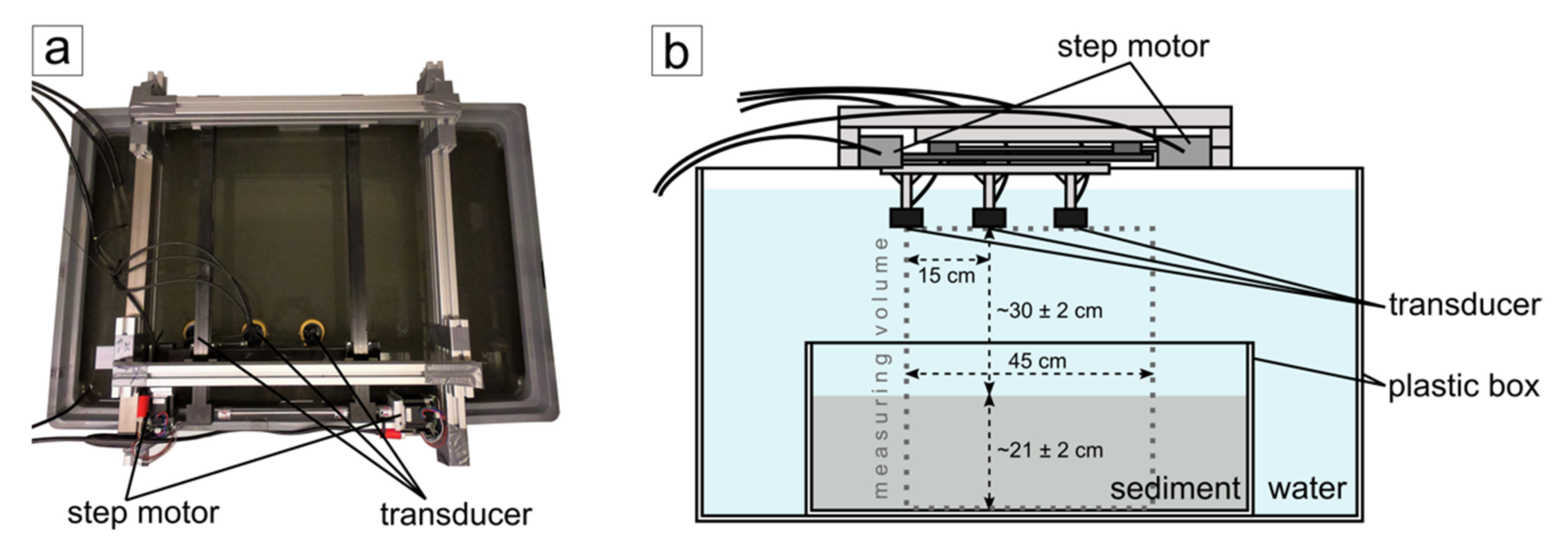
2.1. 3D Seismic Lander System
2.2. Test Setup
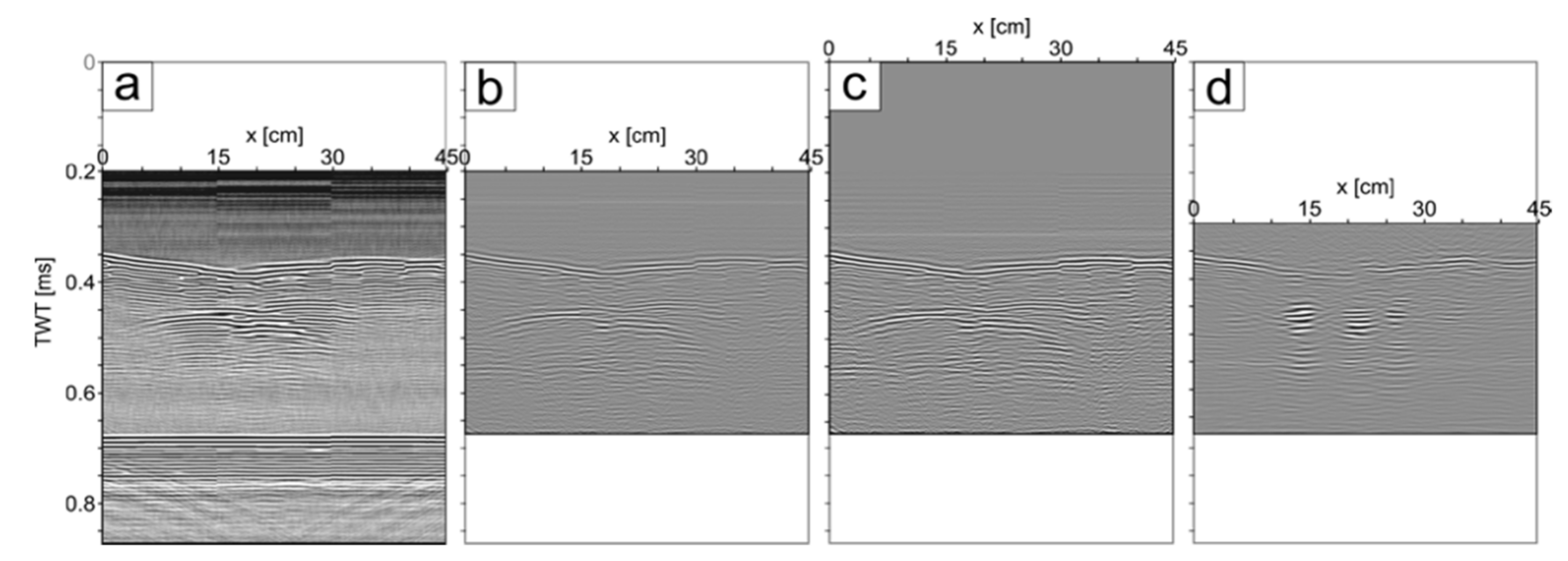
2.3. Processing
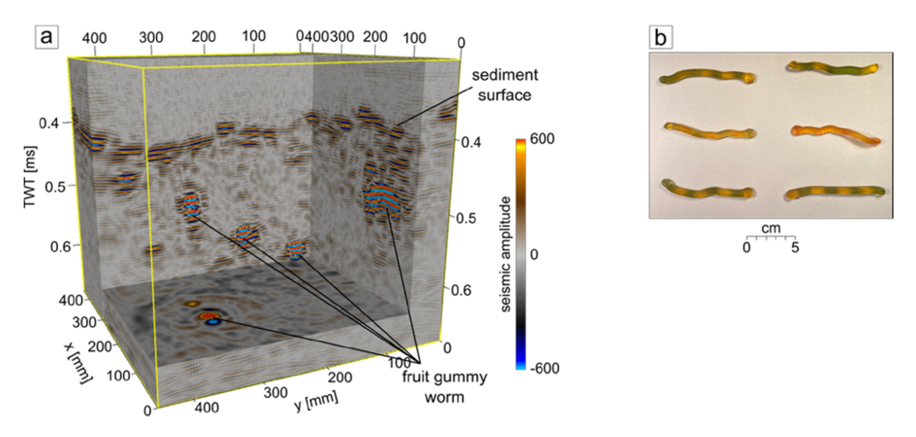
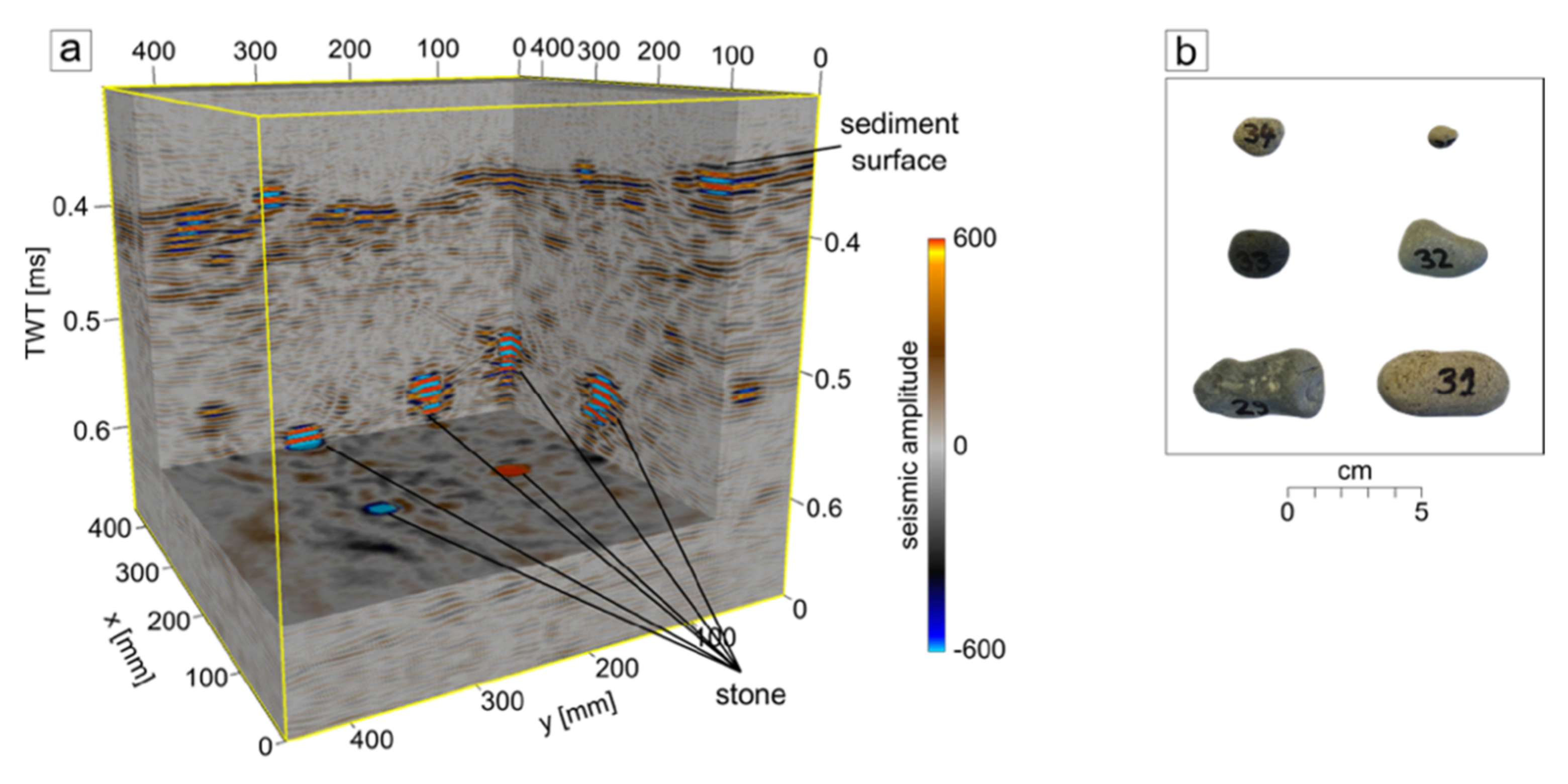
3. Results
4. Discussion
5. Conclusions
Author Contributions
Funding
Data Availability Statement
Acknowledgments
Conflicts of Interest
References
- Von Ziegelmeier, E. Beobachtungen über den Röhrenbau von Lanice conchilega (Pallas) im Experiment und am natürlichen Standort. Helgoländer Wissenschafltiche Meeresunters 1952, IV, 107–129. [Google Scholar] [CrossRef] [Green Version]
- Lyons, A.P. The Potential Impact of Shell Fragment Distributions on High-Frequency Seafloor Backscatter. IEEE J. Ocean. Eng. 2005, 30, 843–851. [Google Scholar] [CrossRef]
- Michaud, E.; Desrosiers, G.; Mermillod-Blondin, F.; Sundby, B.; Stora, G. The functional group approach to bioturbation: II. The effects of the Macoma balthica community on fluxes of nutrients and dissolved organic carbon across the sediment–water interface. J. Exp. Mar. Biol. Ecol. 2006, 337, 178–189. [Google Scholar] [CrossRef]
- Kauppi, L.; Bernard, G.; Bastrop, R.; Norkko, A.; Norkko, J. Increasing densities of an invasive polychaete enhance bioturbation with variable effects on solute fluxes. Sci. Rep. 2018, 8, 7619. [Google Scholar] [CrossRef]
- Eleftheriou, A. Methods for the Study of Marine Benthos; John Wiley & Sons: Hoboken, NJ, USA, 2013. [Google Scholar]
- Jørgensen, L.L.; Renaud, P.E.; Cochrane, S.K.J. Improving benthic monitoring by combining trawl and grab surveys. Mar. Pollut. Bull. 2011, 62, 1183–1190. [Google Scholar] [CrossRef]
- Dück, Y.; Lorke, A.; Jokiel, C.; Gierse, J. Laboratory and field investigations on freeze and gravity core sampling and assessment of coring disturbances with implications on gas bubble characterization. Limnol. Oceanogr. Methods 2019, 17, 585–606. [Google Scholar] [CrossRef]
- Shinn, E.A. Burrowing in Recent Lime Sediments of Florida and the Bahamas. J. Paleontol. 1968, 42, 879–894. [Google Scholar]
- Rhoads, D.C.; Germano, J.D. Characterization of Organism-Sediment Relations Using Sediment Profile Imaging: An Efficient Method of Remote Ecological Monitoring of the Seafloor (RemotsTM System). Mar. Ecol. Prog. Ser. 1982, 8, 115–128. [Google Scholar] [CrossRef]
- Pouliquen, E.; Lyons, A.P. Backscattering from bioturbated sediments at very high frequency. IEEE J. Ocean. Eng. 2002, 27, 388–402. [Google Scholar] [CrossRef]
- Dufour, S.C.; Desrosiers, G.; Long, B.; Lajeunesse, P.; Gagnoud, M.; Labrie, J.; Archambault, P.; Stora, G. A new method for three-dimensional visualization and quantification of biogenic structures in aquatic sediments using axial tomodensitometry. Limnol. Oceanogr. Methods 2005, 3, 372–380. [Google Scholar] [CrossRef]
- Pennafirme, S.F.; Machado, A.S.; Lima, I.; Suzuki, K.N.; Lopes, R.T. Viability of microcomputed tomography to study tropical marine worm galleries in humid muddy sediments. In Proceedings of the 2013 International Nuclear Atlantic Conference—INAC 2013, Recife, Brazil, 24–29 November 2013. [Google Scholar]
- Rosenberg, R.; Grémare, A.; Duchêne, J.C.; Davey, E.; Frank, M. 3D visualization and quantification of marine benthic biogenic structures and particle transport utilizing computer-aided tomography. Mar. Ecol. Prog. Ser. 2008, 363, 171–182. [Google Scholar] [CrossRef]
- Chang, A.; Jung, J.; Um, D.; Yeom, J.; Hanselmann, F. Cost-effective Framework for Rapid Underwater Mapping with Digital Camera and Color Correction Method. KSCE J. Civ. Eng. 2019, 23, 1776–1785. [Google Scholar] [CrossRef]
- Gomes-Pereira, J.N.; Auger, V.; Beisiegel, K.; Benjamin, R.; Bergmann, M.; Bowden, D.; Buhl-Mortensen, P.; De Leo, F.C.; Dionísio, G.; Durden, J.M.; et al. Current and future trends in marine image annotation software. Prog. Oceanogr. 2016, 149, 106–120. [Google Scholar] [CrossRef]
- Beisiegel, K.; Darr, A.; Gogina, M.; Zettler, M.L. Benefits and shortcomings of non-destructive benthic imagery for monitoring hard-bottom habitats. Mar. Pollut. Bull. 2017, 121, 5–15. [Google Scholar] [CrossRef] [PubMed]
- Solan, M.; Germano, J.D.; Rhoads, D.C.; Smith, C.; Michaud, E.; Parry, D.; Wenzhöfer, F.; Kennedy, B.; Henriques, C.; Battle, E.; et al. Towards a greater understanding of pattern, scale and process in marine benthic systems: A picture is worth a thousand worms. J. Exp. Mar. Biol. Ecol. 2003, 285–286, 313–338. [Google Scholar] [CrossRef]
- Brown, C.J.; Smith, S.J.; Lawton, P.; Anderson, J.T. Benthic habitat mapping: A review of progress towards improved understanding of the spatial ecology of the seafloor using acoustic techniques. Estuar. Coast. Shelf Sci. 2011, 92, 502–520. [Google Scholar] [CrossRef]
- Dartnell, P.; Gardner, J.V. Predicting Seafloor Facies from Multibeam Bathymetry and Backscatter Data. Photogramm. Eng. Remote Sens. 2004, 70, 1081–1091. [Google Scholar] [CrossRef] [Green Version]
- Heinrich, C.; Feldens, P.; Schwarzer, K. Highly dynamic biological seabed alterations revealed by side scan sonar tracking of Lanice conchilega beds offshore the island of Sylt (German Bight). Geo-Mar. Lett. 2016, 37, 289–303. [Google Scholar] [CrossRef]
- Schimel, A.C.G.; Brown, C.J.; Ierodiaconou, D. Automated Filtering of Multibeam Water-Column Data to Detect Relative Abundance of Giant Kelp (Macrocystis pyrifera). Remote Sens. 2020, 12, 1371. [Google Scholar] [CrossRef]
- Czechowska, K.; Feldens, P.; Tuya, F.; De Esteban, M.C.; Espino, F.; Haroun, R.; Schönke, M.; Otero-Ferrer, F. Testing Side-Scan Sonar and Multibeam Echosounder to Study Black Coral Gardens: A Case Study from Macaronesia. Remote Sens. 2020, 12, 3244. [Google Scholar] [CrossRef]
- Feldens, P.; Schulze, I.; Papenmeier, S.; Schönke, M.; Von Deimling, J.S. Improved Interpretation of Marine Sedimentary Environments Using Multi-Frequency Multibeam Backscatter Data. Geosciences 2018, 8, 214. [Google Scholar] [CrossRef]
- Held, P.; Von Deimling, J.S. New Feature Classes for Acoustic Habitat Mapping—A Multibeam Echosounder Point Cloud Analysis for Mapping Submerged Aquatic Vegetation (SAV). Geosciences 2019, 9, 235. [Google Scholar] [CrossRef] [Green Version]
- Janowski, L.; Trzcinska, K.; Tegowski, J.; Kruss, A.; Rucinska-Zjadacz, M.; Pocwiardowski, P. Nearshore Benthic Habitat Mapping Based on Multi-Frequency, Multibeam Echosounder Data Using a Combined Object-Based Approach: A Case Study from the Rowy Site in the Southern Baltic Sea. Remote Sens. 2018, 10, 1983. [Google Scholar] [CrossRef] [Green Version]
- Lurton, X.; Lamarche, G.; Brown, C.; Lucieer, V.; Rice, G.; Schimel, A.; Weber, T. Backscatter Measurements by Seafloor-Mapping Sonars: Guidelines and Recommendations. 2015, p. 200. Available online: https://niwa.co.nz/static/BWSG_REPORT_MAY2015_web.pdf (accessed on 8 December 2021).
- Planke, S.; Erikson, F.N.; Berndt, C.; Mienert, J.; Masson, D.G. P-Cable High-Resolution Seismic. Oceanography 2009, 22, 85. [Google Scholar] [CrossRef]
- Marsset, B.; Missiaen, T.; De Roeck, J.M.; Noblem, M.; Versteeg, R.J.; Henriet, J.P. Very high resolution 3D marine seismic data processing for geotechnical applications. Geophys. Prospect. 1998, 46, 105–120. [Google Scholar] [CrossRef]
- Wilken, D.; Wunderlich, T.; Hollmann, H.; Schwardt, M.; Rabbel, W.; Mohr, C.; Schulte-Kortnack, D.; Nakoinz, O.; Enzmann, J.; Jürgens, F.; et al. Imaging a medieval shipwreck with the new PingPong 3D marine reflection seismic system. Archaeol. Prospect. 2019, 26, 211–223. [Google Scholar] [CrossRef]
- Wilken, D.; Wunderlich, T.; Feldens, P.; Coolen, J.; Preston, J.; Mehler, N. Investigating the Norse Harbour of Igaliku (Southern Greenland) Using an Integrated System of Side-Scan Sonar and High-Resolution Reflection Seismics. Remote Sens. 2019, 11, 1889. [Google Scholar] [CrossRef] [Green Version]
- Gutowski, M.; Malgorn, J.; Vardy, M. 3D sub-bottom profiling—high resolution 3D imaging of shallow subsurface structures and buried objects. In Proceedings of the OCEANS 2015—Genova, Genova, Italy, 18–21 May 2015; pp. 1–7. [Google Scholar] [CrossRef]
- Wildman, R.A.; Huettel, M. Acoustic detection of gas bubbles in saturated sands at high spatial and temporal resolution: Acoustic detection of bubbles in sand. Limnol. Oceanogr. Methods 2012, 10, 129–141. [Google Scholar] [CrossRef]
- Orr, M.H.; Rhoads, D.C. Acoustic imaging of structures in the upper 10 cm of sediments using a megahertz backscattering system: Preliminary results. Mar. Geol. 1982, 46, 117–129. [Google Scholar] [CrossRef]
- Suganuma, H.; Mizuno, K.; Asada, A. Application of wavelet shrinkage to acoustic imaging of buried asari clams using high-frequency ultrasound. Jpn. J. Appl. Phys. 2018, 57, 07LG08. [Google Scholar] [CrossRef]
- Mizuno, K.; Liu, X.; Katase, F.; Asada, A.; Murakoshi, M.; Yagita, Y.; Fujimoto, Y.; Shimada, T.; Watanabe, Y. Automatic non-destructive three-dimensional acoustic coring system for in situ detection of aquatic plant root under the water bottom. Case Stud. Nondestruct. Test. Eval. 2016, 5, 1–8. [Google Scholar] [CrossRef] [Green Version]
- Mizuno, K.; Yu, Z.; Murakoshi, M.; Suganuma, H.; Asada, A.; Fujimoto, Y.; Takahashi, Y.; Shimada, T. Survey of the Lotus Root Habitats in the Sediment Using Acoustic Coring System. In Proceedings of the 2018 OCEANS-MTS/IEEE Kobe Techno-Oceans, Kobe, Japan, 28–31 May 2018; pp. 1–5. [Google Scholar]
- Dorgan, K.M.; Ballentine, W.; Lockridge, G.; Kiskaddon, E.; Ballard, M.S.; Lee, K.M.; Wilson, P.S. Impacts of simulated infaunal activities on acoustic wave propagation in marine sediments. J. Acoust. Soc. Am. 2020, 147, 812–823. [Google Scholar] [CrossRef]
- Leighton, T.G.; Evans, R.C.P. The detection by sonar of difficult targets (including centimetre-scale plastic objects and optical fibres) buried in saturated sediment. Appl. Acoust. 2008, 69, 438–463. [Google Scholar] [CrossRef]
- Schwinghamer, P.; Guigne, J.Y.; Siu, W.C. Quantifying the impact of trawling on benthic habitat structure using high resolution acoustics and chaos theory. Can. J. Fish. Aquat. Sci. 1996, 53, 288–296. [Google Scholar] [CrossRef]
- Stockwell, J.W. The CWP/SU: Seismic Un∗x package. Comput. Geosci. 1999, 25, 415–419. [Google Scholar] [CrossRef]
- Thomas, M.H.; SegyMAT. Zenodo. Available online: http://0-doi-org.brum.beds.ac.uk/10.5281/zenodo.1305289 (accessed on 8 December 2021).
- Stolt, R.H. Migration by fourier transform. Geophysics 1978, 43, 23–48. [Google Scholar] [CrossRef]
- Yilmaz, Ö. Seismic Data Analysis: Processing, Inversion, and Interpretation of Seismic Data; Society of Exploration Geophysicists: Houston, TX, USA, 2001. [Google Scholar]
- Zettler, M.L.; Alf, A. Bivalvia of German Marine Waters of the North and Baltic Seas; ConchBooks: Harxheim, Germany, 2021. [Google Scholar]
- Tauber, F.; Lemke, W.; Endler, R. Map of Sediment Distribution in the Western Baltic Sea (1: 100,000), Sheet Falster—Mon. Dtsch. Hydrogr. Z. 1999, 51, 27. [Google Scholar] [CrossRef]
- Nickell, L.A.; Black, K.D.; Hughes, D.J.; Overnell, J.; Brand, T.; Nickell, T.D.; Breuer, E.; Harvey, S.M. Bioturbation, sediment fluxes and benthic community structure around a salmon cage farm in Loch Creran, Scotland. J. Exp. Mar. Biol. Ecol. 2003, 285-286, 221–233. [Google Scholar] [CrossRef]
- Michaud, E.; Desrosiers, G.; Mermillod-Blondin, F.; Sundby, B.; Stora, G. The functional group approach to bioturbation: The effects of biodiffusers and gallery-diffusers of the Macoma balthica community on sediment oxygen uptake. J. Exp. Mar. Biol. Ecol. 2005, 326, 77–88. [Google Scholar] [CrossRef]
- Wetzel, A.; Werner, F.; Stow, D. Bioturbation and Biogenic Sedimentary Structures in Contourites. Dev. Sedimentol. 2008, 60, 183–202. [Google Scholar] [CrossRef]
- Stanton, T.K.; Chu, D. On the acoustic diffraction by the edges of benthic shells. J. Acoust. Soc. Am. 2004, 116, 239–244. [Google Scholar] [CrossRef] [PubMed] [Green Version]
- Stief, P.; Poulsen, M.; Nielsen, L.P.; Brix, H.; Schramm, A. Nitrous oxide emission by aquatic macrofauna. Proc. Natl. Acad. Sci. USA 2009, 106, 4296–4300. [Google Scholar] [CrossRef] [PubMed] [Green Version]
- Lurton, X. An Introduction to Underwater Acoustics: Principles and Applications, 2nd ed.; Springer Science & Business Media: Chichester, UK, 2010. [Google Scholar]
- Gay, A.; Mourgues, R.; Berndt, C.; Bureau, D.; Planke, S.; Laurent, D.; Gautier, S.; Lauer, C.; Loggia, D. Anatomy of a fluid pipe in the Norway Basin: Initiation, propagation and 3D shape. Mar. Geol. 2012, 332–334, 75–88. [Google Scholar] [CrossRef]


| Time Slice [ms TWT] | Q1 (Undisturbed) | Q2 (Spatula Cross) | Q3 (Disturbed) | Q4 (Disturbed < 0.1 ms TWT) |
|---|---|---|---|---|
| 0.35–0.68 | 123.3 (27.7) | 119.5 (32.1) | 129.9 (32.2) | 128.6 (26.0) |
| 0.45–0.50 | 91.5 (27.3) | 100.5 (35.3) | 113.6 (60.3) | 99.9 (27.9) |
| 0.50–0.55 | 70.1 (22.5) | 80.1 (43.4) | 92.3 (44.2) | 67.8 (22.5) |
| 0.55–0.60 | 56.4 (36.0) | 68.2 (61.0) | 84.4 (60.6) | 75.7 (75.5) |
Publisher’s Note: MDPI stays neutral with regard to jurisdictional claims in published maps and institutional affiliations. |
© 2021 by the authors. Licensee MDPI, Basel, Switzerland. This article is an open access article distributed under the terms and conditions of the Creative Commons Attribution (CC BY) license (https://creativecommons.org/licenses/by/4.0/).
Share and Cite
Schulze, I.; Wilken, D.; Zettler, M.L.; Gogina, M.; Schönke, M.; Feldens, P. Laboratory Measurements to Image Endobenthos and Bioturbation with a High-Frequency 3D Seismic Lander. Geosciences 2021, 11, 508. https://0-doi-org.brum.beds.ac.uk/10.3390/geosciences11120508
Schulze I, Wilken D, Zettler ML, Gogina M, Schönke M, Feldens P. Laboratory Measurements to Image Endobenthos and Bioturbation with a High-Frequency 3D Seismic Lander. Geosciences. 2021; 11(12):508. https://0-doi-org.brum.beds.ac.uk/10.3390/geosciences11120508
Chicago/Turabian StyleSchulze, Inken, Dennis Wilken, Michael L. Zettler, Mayya Gogina, Mischa Schönke, and Peter Feldens. 2021. "Laboratory Measurements to Image Endobenthos and Bioturbation with a High-Frequency 3D Seismic Lander" Geosciences 11, no. 12: 508. https://0-doi-org.brum.beds.ac.uk/10.3390/geosciences11120508