
Integration of Geophysical Methods for Doline Hazard Assessment: A Case Study from Northern Oman


1
Department of Earth Science, Sultan Qaboos University, Muscat 123, Oman
2
School of Mineral Resources Engineering, Technical University of Crete, 73100 Chania, Greece
3
Department of Earth Sciences and Environment, Prince El Hassan Bin Talal Faculty for Natural Resources & Environment, The Hashemite University, P.O. Box 330127, Zarqa 13113, Jordan
*
Author to whom correspondence should be addressed.
Geosciences 2022, 12(6), 243; https://0-doi-org.brum.beds.ac.uk/10.3390/geosciences12060243
Submission received: 9 April 2022
/
Revised: 2 June 2022
/
Accepted: 5 June 2022
/
Published: 13 June 2022
(This article belongs to the Special Issue Ground Penetrating Radar Velocities)
Abstract
:Subsurface formations with low compaction, often, due to the presence of underlying cavities, are potential sources of hazards. Thus, understanding the occurrence, properties, and extension of these weak zones poses a major concern in engineering geophysics. In this study, we examine the ability of geophysical methods to map weak areas over carbonates in Northern Oman. The weak zones are known to cause surface depression in many areas. The geophysical methods examined involve Ground-Penetrating Radar (GPR), Seismic Refraction Tomography (SRT), and Electrical Resistivity Tomography (ERT). This integrated geophysical survey was conducted near the Bimmah sinkhole, in the Quriya area, Northern Oman. The survey covers both an area with ground truth (low compaction sediments overlaying a cave) and a part with unknown subsurface properties. GPR velocity analysis using selected diffraction’s fitting helped to identify high-velocity anomalies that were attributed to the cavity. The GPR interpretation was calibrated with SRT and ERT. The former showed a clear drop in P-wave velocity and low ray coverage at the cavity zone, while the latter demonstrated high resistivity anomalies caused by the air filling the cavity. The scope was to examine the geophysical methods response, especially the GPR, and utilize the results of this preliminary approach for a wider exploration investigation in the area. The results from the study indicated that the GPR is capable to serve as a pioneer method in detecting the cavities. Hence, the GPR will cover large area in the site and the other two methods will be used as complementary for the final subsurface conditions’ evaluation.
1. Introduction
In carbonate karst environments, caves are formed by the chemical and physical interaction between groundwater with the rock. These geologic features do not follow a readily distinguishable pattern and represent a major source of hazard in populated areas underlain by carbonate rocks. The changes of the physical and chemical properties of the host rock usually produce a bulk disturbance volume that can be larger than the cave itself. This may help geophysical methods to detect the cavities hidden in subsurface [1,2,3]. Over the last two decades, the use of geophysical methods for karst detection and characterization has drastically increased. This increase is due partly to the recent technological developments in data acquisition, field equipment and procedures, recently developed forward and reverse modeling workflows of data, as well as advances in interpretation and visualization techniques [4].
Experience has shown that the knowledge of geometry and the structure of the different parts of a karstic voids system usually involves many uncertainties because of the complex nature of karst systems [1,5]. Additionally, when there is a strong contrast in physical properties between the cave and the host rock, the inverted models are more divergent and poorly fit the observed data which makes the solutions less reliable [2,6]. This makes the integration of various geophysical methods to become a necessity.
The combination of ERT with GPR or seismic methods has been used worldwide during the last two decades. Most of the combinations aimed to locate groundwater-saturated zones or cavity occurrences. Among many others, there are examples from Spain (e.g., [2]), Iran (e.g., [7]), Oman [4,8,9], Turkey (e.g., [10]), China [11], and from the US [12]. Ref. [13] described geophysical methods adapted to karst study in a general book on karst hydrogeology. In addition, [5] collected 25 papers dealing with different aspects of karsts, their geology, geomorphology, modeling, and exploration methods.
Still, the main target of detecting caves and voids in karstic areas is the possible existence of a doline above the void or the potential of the area above the void to create weak zones which may lead to dolines visible on the surface, such as sinkholes. Sinkhole mapping and characterization are implemented by geophysical methods to reduce the potential of subsistence [14,15]. The problem is that, when a sinkhole appears, the subsurface is already disturbed. Thus, there is a need to detect dolines or areas with the potential to produce dolines or sinkholes [16,17].
There are only a few published studies in the literature that document the use of geophysical methods for karstic terrains in Oman. For example, [18] used Micro-gravity and VLF to detect cavities in Wadi-Shab, North Oman. Ref. [8] used GPR to detect karstic features in carbonate rocks in a coastal area in Northern Oman. Ref. [9] used GPR, resistivity and Multi-channel Surface Analysis of Surface Wave (MASW) to detect natural karstic features in the Duqm area, Northern Oman.
Here, we combine three geophysical methods—namely, the Ground-Penetrating Radar (GPR), the Electrical Resistivity Tomography (ERT), and the Seismic Refraction Tomography (SRT)—to evaluate the first 10 m of the subsurface in a pilot study over a known cave and a known disturbed with a low compaction overburden. The pilot study area is next to a known sinkhole in Quriat, Northern Oman. These are the preliminary results of a future large-scale exploration in the extended area to be used as a guide for the assessment methodology and geophysical parameters. We show that the use of the GPR method as a pioneering method can produce an adaptive electromagnetic (EM) velocity attribute, which after our calibration with seismic velocity and electrical resistivity sections can further involve the latter two methods as complementary and only at selected areas. This is essential as the GPR method is the one with the lowest acquisition duration, processing and is relatively easily applied in the field.
2. Area and Geological Background
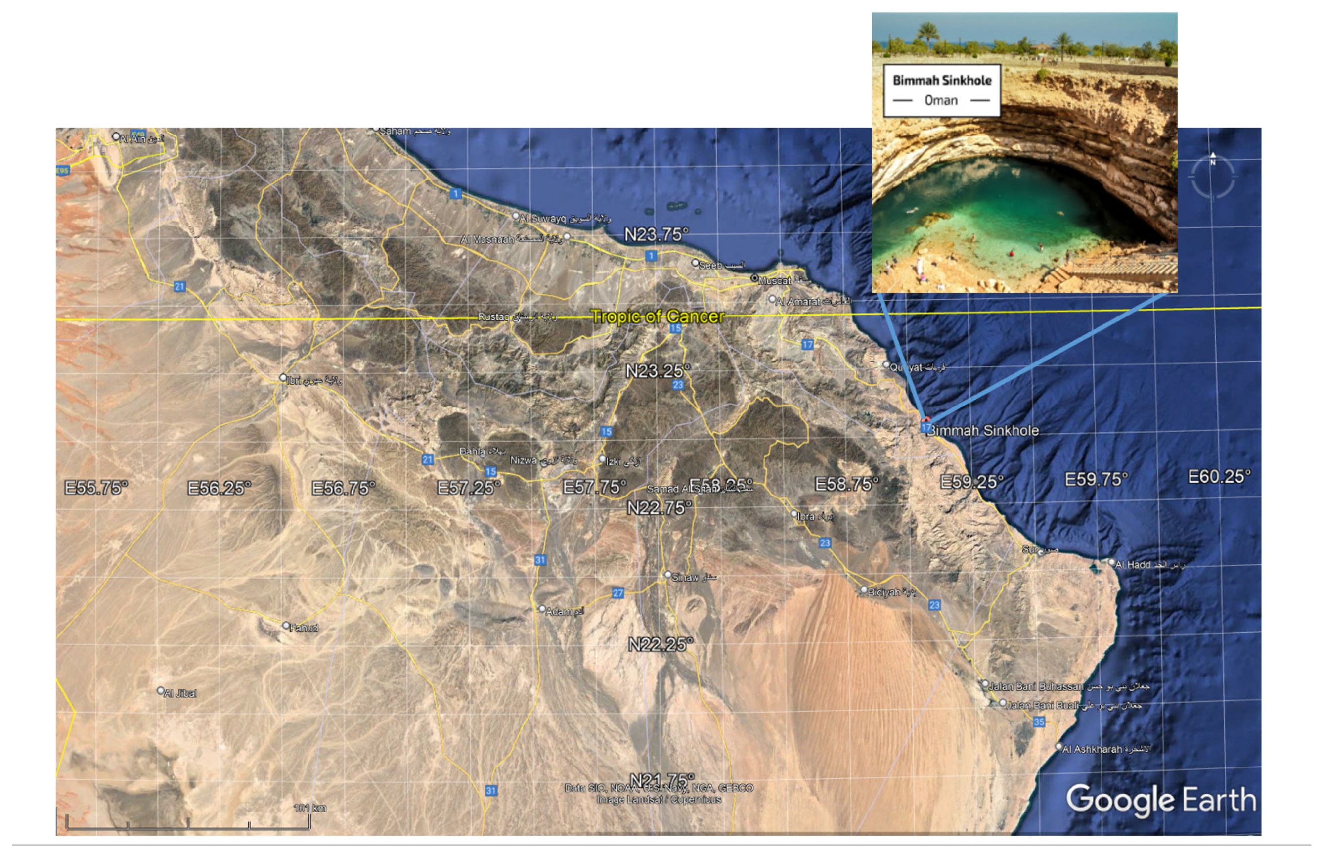
The studied area is located in Quriat. It is a flat coastal plain with individual inselbergs of predominantly carbonate rocks deposited under a shallow marine environment during the Tertiary [19]. The terrain is physio-graphically karstified with a plain area that extends for about 2 km between encapsulating elevated mountains and the coast of the Arabian Sea. The Bimmah sinkhole is a remarkable karstic feature located in the plain a few meters to the coast (Figure 1).
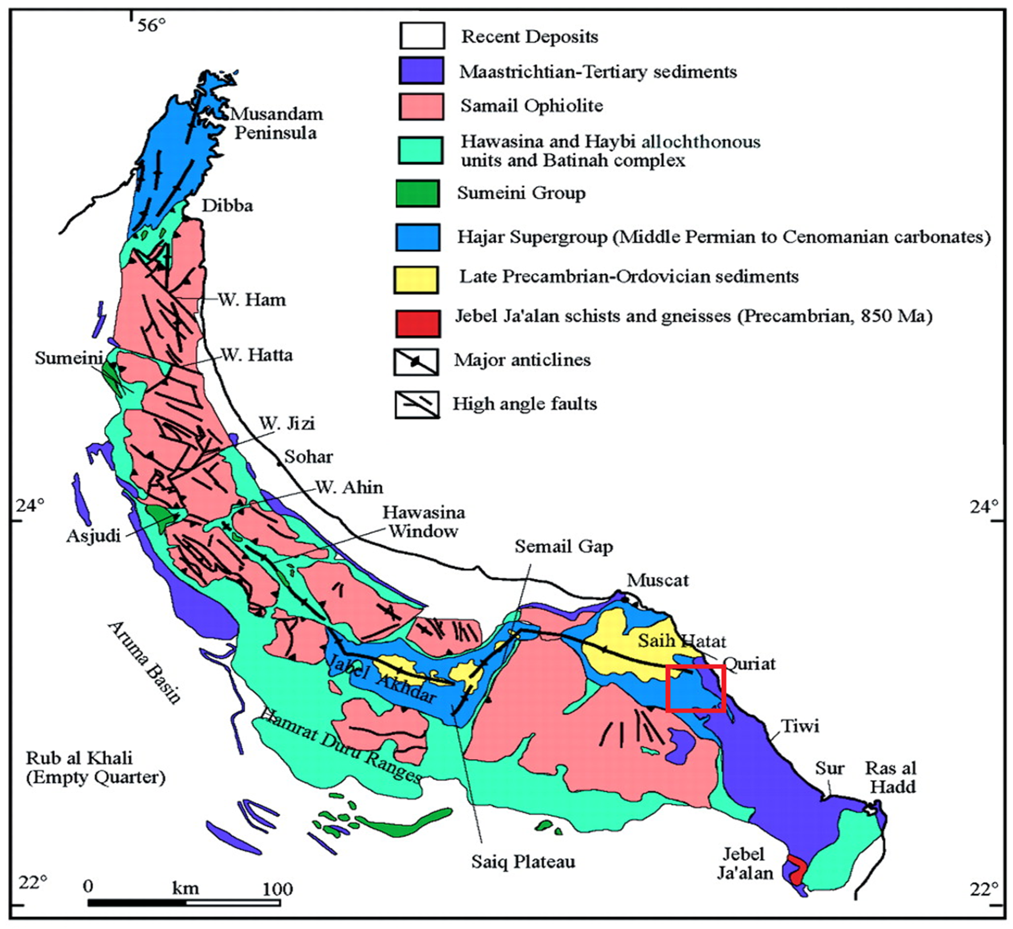
Figure 2 is a simplified geological map of North Oman, which includes the study area and its environs (modified after [20]). The Tertiary rock succession in Quriat consists of a number of formations ascribed to three stratigraphic groups: the Hadhramaut, the Dhofar, and Fars Groups [21]. To the east, the succession is relatively thin (200–300 m) and comprised of shelf limestone of the Seeb (Hadhramaut Group) and Shama Formations (Dhofar Group). In central locations, the Tertiary limestone is exceptionally thick (2500–3500 m), with a massive basal unit comprised of restricted shelf facies limestone of the Jafnayn Formation overlain by several formations belonging to the Hadhramaut Group and slope deposits from the Dhofar Group [19,21]. Thin deposits belonging to the Fars Group complete the succession. To the west, the Tertiary succession is made up of shelf deposits of the Hadhramaut Group, comprising the Jafnayn Formation (Late Paleocene–Early Eocene), the Rus Formation (Eocene), and the Seeb Formation (Middle Eocene). The Jafnayn Formation consists of massive bioclastic limestone with subordinate conglomerate, sandstone and glauconitic marl forming a series of limestone mesas. The sandstone and marl are inter-layered with nodular and bioclastic limestone containing abundant algal debris and crushed fragments of benthic foraminifera, mainly alveolinidae [21].
3. Methods, Data Acquisition, and Processing
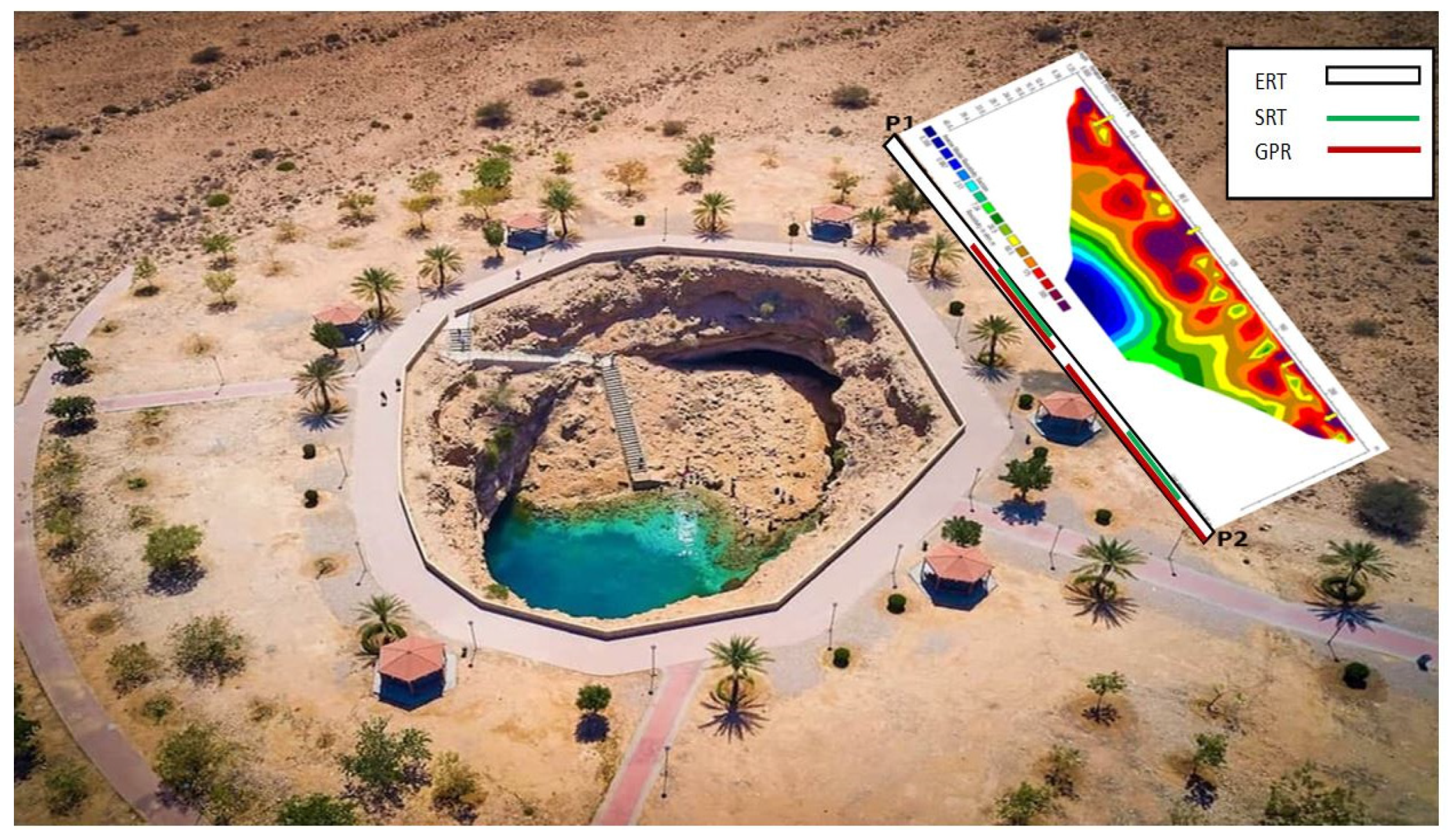
A large cavity, visible within the Bimmah sinkhole, continues at more than 100 m and extended laterally into the subsurface [22,23] (Figure 3). The cavity system in the area consists of two parts. The first part is filled with air. It starts at around 7 m below the surface and ends at around 18–20 m. From this depth and below, the cavity is filled with very saline water. In order to make a direct comparison between the used methods, the survey lines were all acquired along a profile above the cavity (black rectangle, green and red lines in Figure 3).
3.1. Electrical Resistivity Tomography
The ERT method is one of the geophysical methods that have proven efficient with increasing successful applications in many areas around the globe including Oman. The ERT method involves determining subsurface resistivity distribution by taking ground surface measurements; it is based on Ohm’s law. The direct current is injected into the ground by one pair of electrodes, and a second pair is used to measure the resulting potential difference [24]. Two-dimensional electrical resistivity imaging is gaining increasing acceptance among other investigation methods used for detecting karstic features [25]. ERT applications in cavity detection have been documented in numerous published studies from all over the world (e.g., [4,24,25,26,27]). Typically, the appearance of weak zones in resistivity tomograms depends on the lithology of the host rock, its saturating fluids, and the geometry of the cavity [2]. Cavities can be seen as high resistivity anomalies if the cavity is filled with air [2] or low resistivity anomalies if it is filled with salt water [4,28]. Disturbed overburden with low compaction on the other hand may be surveyed as a relatively low resistivity zone if moisture is present, or relatively higher than the surrounding’s resistivity area if the subsurface is dry. The latter is the case for the studied site.
For the ERT survey, we implemented the Wenner–Schlumberger configuration in the data collection. In this configuration, four electrodes are used, two outer and two inner ones. The two outer electrodes are used to inject the current, whereas the two inner electrodes are used as potential electrodes. The array used here is more sensitive to depth resistivity variations than the dipole–dipole array, but it has a much higher Signal-to-Noise Ratio (SNR) than the dipole–dipole array. Ref. [29] reported the efficiency of the Wenner-Schlumberger over the Wenner and the dipole–dipole arrays for the mapping of vertically and laterally varying heterogeneities within different types of rocks. Even though, the dipole–dipole array is more sensitive to lateral electrical resistivity changes, it has been observed that strong resistivity contrast may produce misplacement of the subsurface anomalies, with the additional effect that this array may increase lateral resistivity heterogeneity, even for a layered earth.
The measuring device is constituted by a resistivity meter connected to an arrangement of 48 electrodes with an electrode spacing of 5 m (maximum depth of 45 m). The measured apparent resistivity data were inverted to produce a resistivity model of the subsurface using iterative smoothness-constrained least squares [30,31]. This inversion scheme requires no previous knowledge of the subsurface; the initial guess model is constructed directly from field measurements. Then, the ERT tomographic method iterates and compares the calculated apparent resistivity to the measured apparent resistivity, modifying the resistivity section and repeating the process until the difference between calculated and measured resistivities reach its minimum (Figure 4).
3.2. Seismic Refraction
Seismic refraction methods are based on Snell’s law, which governs the refraction of propagating waves across the boundary between layers of different physical properties. The arrival times of those waves once recorded at the surface can be inverted to derive the properties of the rock along which they have traveled [24,32]. Examples of such properties include rock velocities, depths, and thicknesses among many more physical and elastic properties. Conventional refraction inversion methods use a “layer cake” approach. In the latter approach, a subsurface model will be built in a form of a number of continuous constant velocity layers with velocities and thicknesses that are varied through interactive forward modeling in an effort to reduce the misfit between the theoretical travel times and the ones from the field data. These methods require that sections of the travel time curves be mapped to a refractor, a task that can be difficult at best in karst situations [33].
Unlike conventional refraction methods, in Seismic Refraction Tomography (SRT), the model is made up of a high number of small constant velocity grid cells or nodes. The inversion is performed by an automated procedure that involves the tracing of rays through an initially built model, the comparison of the modeled travel times with the ones derived from field data, and then adjusting the model grid by grid in order to find the best fit between the theoretical and real-time picks. In the end, a final model close to the earth will be produced. A key advantage of SRT is that because there is no assumption of continuous constant velocity layers, SRT can help model localized velocity anomalies.
Refs. [33,34] demonstrated that the most basic requirement for detecting a cavity or a very weak zone in a medium with relatively high seismic velocity is to have adequate ray coverage in the area surrounding the anomaly [33]. In other words, energy must have a path back to the surface in order to be recorded. With the above indicators (low velocity and low ray coverage for low seismic velocities within high seismic velocities), SRT has demonstrated successful applications in interpreting shallow subsurface geology (e.g., [2,28,33,35]).
Seismic data were collected at two places along the ERT study line (Figure 3). One spread was surveyed over the known cavity with the disturbed overburden and one away from the cavity. The cavity can be visited and its existence signature within the ERT profile was verified, so the second location was chosen based on the ERT results, and it was surveyed in an area of relatively low electrical resistivity where no doline was expected. Twenty-four geophones of 4.5 Hz have been used for each spread with a geophone spacing of 1.5 m. With this spread length, the refraction method can show reliable features for up to a 10-m depth, which is sufficient in our case. The energy source used in the acquisition is a 5-kg hammer, along with a metallic plate. It was ensured that the best results were obtained by stacking the recorded signal five times on the seismograph.
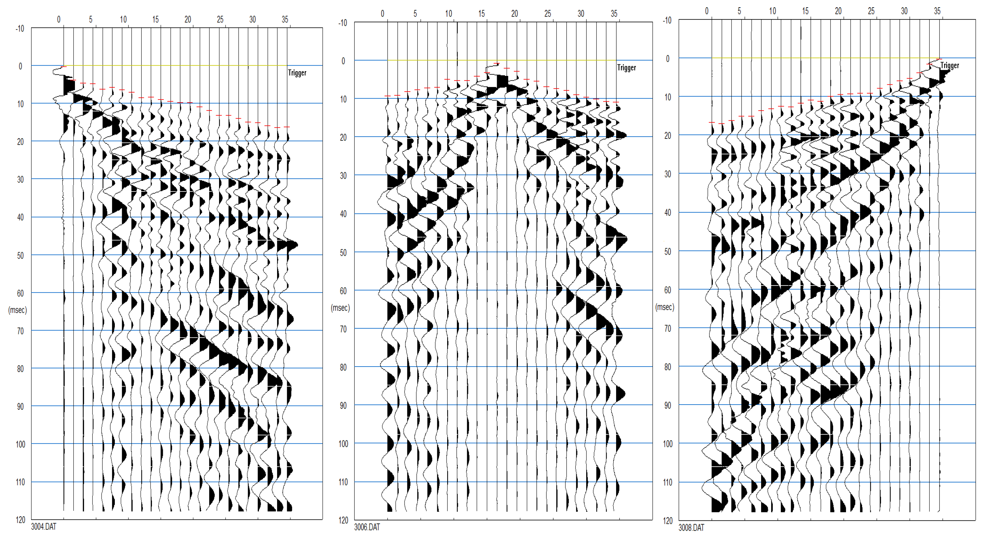
The acquired data were of reasonably good quality and there was no need for any prior filtering. Figure 5 shows some selected shots with the first break. Data were analyzed using Zond2D seismic refraction tomography software. The first processing step consists of picking the first break arrivals of each shot point from both lines. The picking was performed semi-automatically. The first arrival times have been used to build an initial model required for the tomographic inversion. The travel times will also be utilized to estimate the close minimum and maximum velocities with 30% added to the maximum value. In our case, the minimum and maximum velocities were approximated to be around 300 m/s (air wave) and 3500 m/s, respectively. Then, the tomographic method involves the iterative tracing of rays through the built model, the comparison of the calculated travel times with the measured travel times and updating of the model. The process will be repeated until the difference between calculated and measured times will reach a minimum global Root Mean Square (RMS) error. The latter RMS error integrates all errors between calculated and measured travel times in the least square meaning (Figure 6).
3.3. Ground-Penetrating Radar
GPR is one of the very common non-destructive geophysical methods that are widely used in near-surface mapping purposes. The principles of the EM waves propagation are similar to those of the seismic method, but in GPR surveying, the reflections or diffractions are caused by layers or small heterogeneities with different dielectric properties [36]. GPR allows fast and dense data collection in remote areas, as well as in the urban environment. The depth of penetration of the GPR depends heavily on the frequency of the radar signal, as well as the electrical properties of the substrate. GPR has a wide range of applications for shallow subsurface investigations in engineering geophysics, such as mineral exploration, geological, geotechnical, hydrogeological, environmental, and archeological studies [4,27,37]. Of particular usage of GPR is the geologic characterization of the subsurface materials, as well as for the mapping of non-geologic objects. The technique is found useful in cavity detection because the presence of cavities can cause drastic changes in rock dielectric permittivity. The cavities expressions in GPR images, depending on their size and the contrast they leave in the host rock. Large cavities may exhibit strong reflections that imitate their geomorphology, while small cavities show hyperbolic diffraction reflections [2,8,9]. Cavities can also appear in a form of amplitude shadow zones [37].
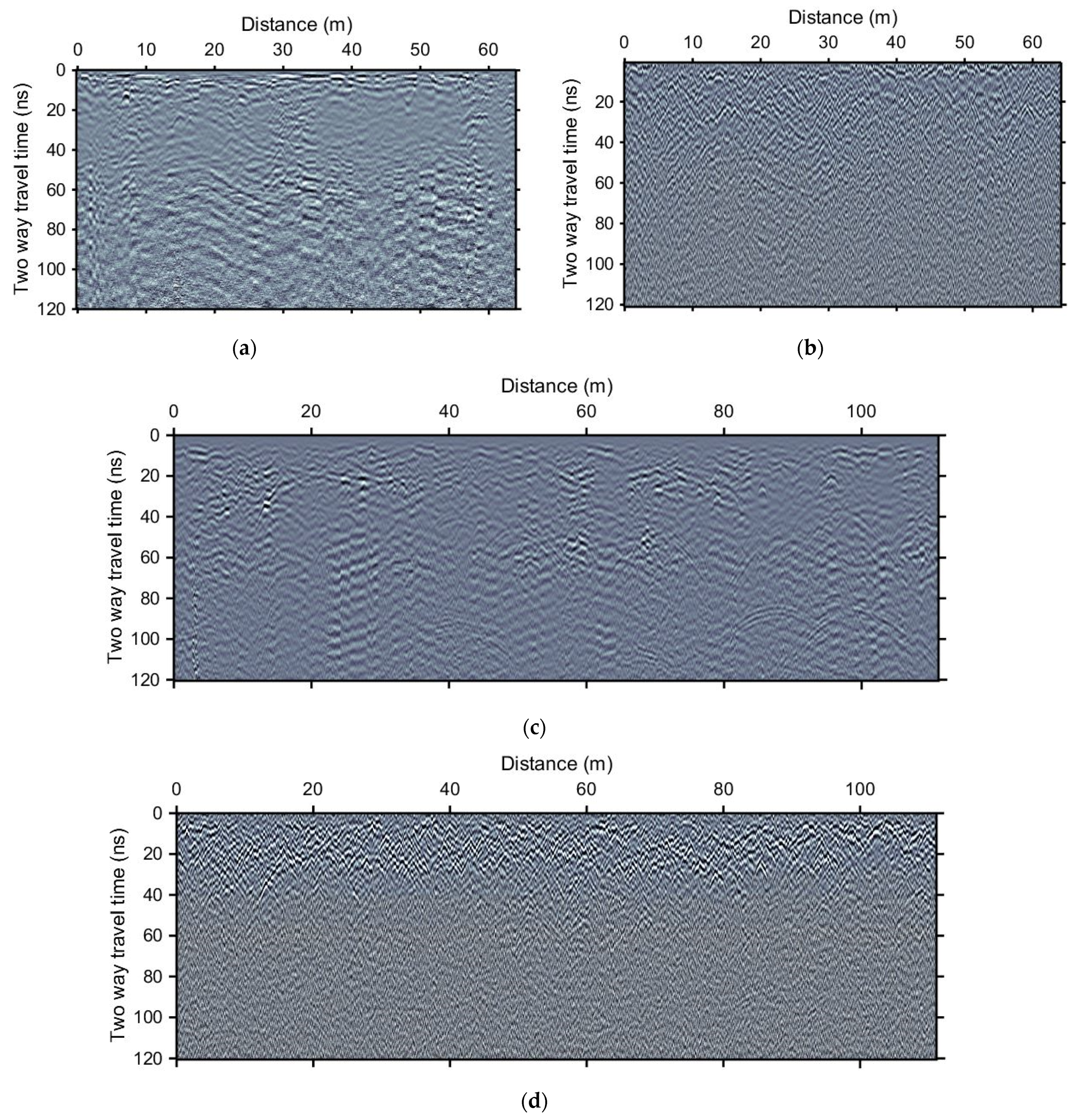
The GPR survey was conducted using the SIR-3000 system. Two antennas 270 MHz, and 400 MHz were tested, and the 270-MHz has shown a good penetration with a reasonable resolution, with an estimated wavelength of around 30 cm. Therefore, the lower dominant frequency GPR data were processed and presented here. The GPR survey was conducted along the resistivity and seismic profiles over and away from the cavity (Figure 3). The time and space intervals were set to 0.1466 ns and 0.02 m, respectively. Conventional processing, using the freeware package MatGPR [38], involved time-zero adjustment, DC removal, Dewow, 300 traces mean trace removal, inverse amplitude decay gain and a band-pass filter of 70 MHz–485 MHz (Figure 7a,c). Our scope was to estimate GPR velocities, so we further applied the plane wave destruction (PWD) method, as introduced by [39], in order to enhance the diffractions and partially eliminate the reflections (Figure 7b,d). Note several air diffractions at the section depicted in Figure 7c and at late times (more than 80 ns, at 40 m, 65 m, 90 m and 100 m from the study line origin), which may cause ambiguities in the velocity analysis [2,27]. Hopefully, due to their relatively small dips, these features are suppressed by the plane wave destruction filtering, along with any reflection energy (Figure 7d). PWD required the estimation of the local slope in the way that it was applied by [40].
For the PWD filtering, first, the local slopes σ of the GPR section are estimated using the local plane wave equation [39]
where P is the wavefield, and x and t are the space and time variables. A 4-point stencil is utilized for the implementation of the partial derivatives in x and t directions for Equation (1) and the PWD filtering. The partial derivatives are smoothed by a triangular smoother before estimating σ [39,40,41]. Even though we utilize the method of [40] for the estimation of the local slopes, for the focusing evaluation, we use the criterion as presented by [42], based on the Fomel’s implementation [43]. For this, the GPR section undergoes to sequential constant velocity time migration within a range of 0.04 m/ns up to 0.20 m/ns, with 0.005 m/ns steps. The amplitudes of the signal are evaluated for each one of the migrated sections in x-t windows using the focusing criterion of the varimax norm [43].
The varimax, φ, is estimated in x-t windows of the migrated GPR signals. Thus, xi represents an abstract vector of the migrated section. To create an abstract vector from a x-t window of the GPR section, each column’s (i.e., each partial trace) elements are arranged one below the other to conclude a column vector of size n. The varimax norm of Equation (2) is related to kurtosis of zero-mean signals, so to ensure this condition we have
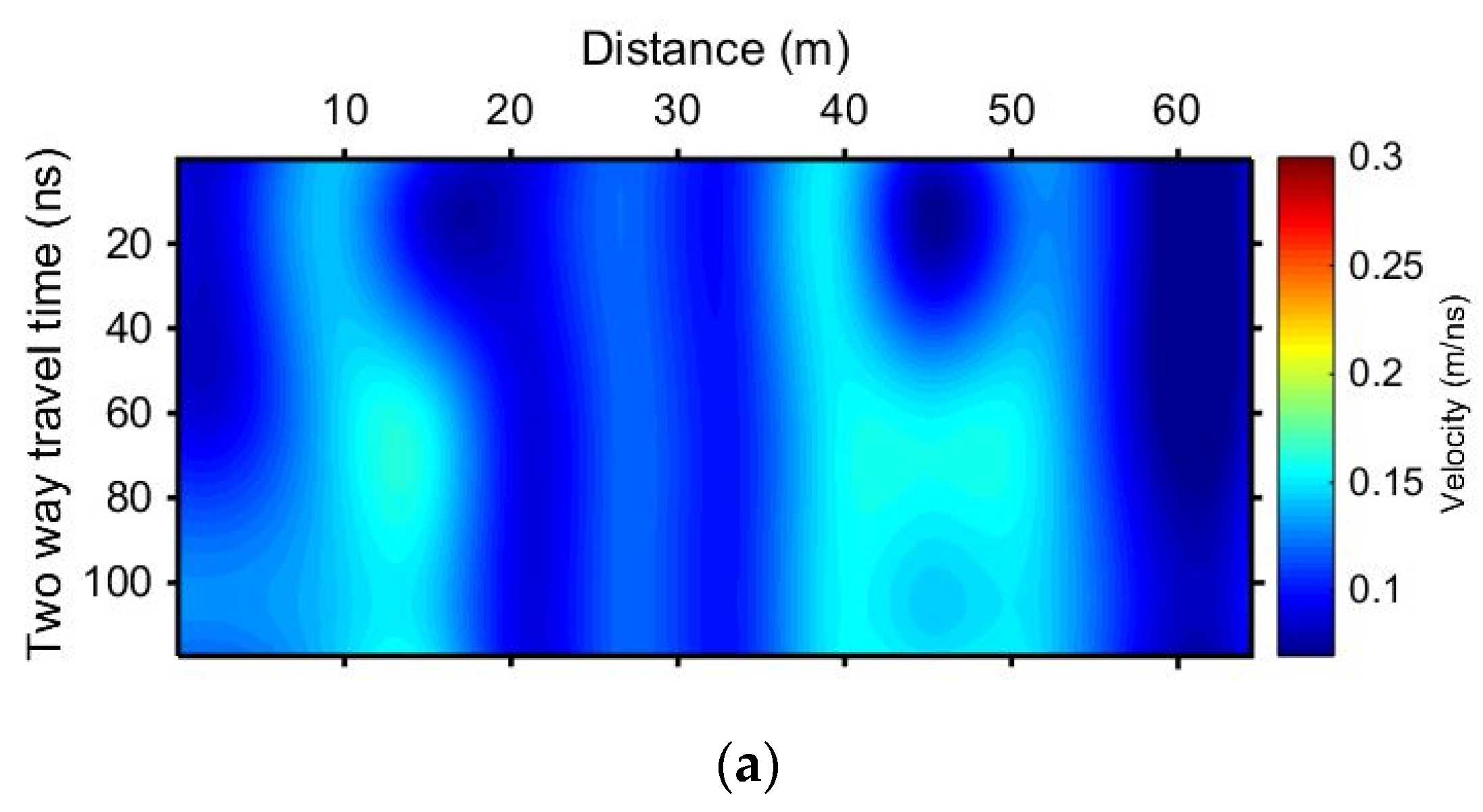
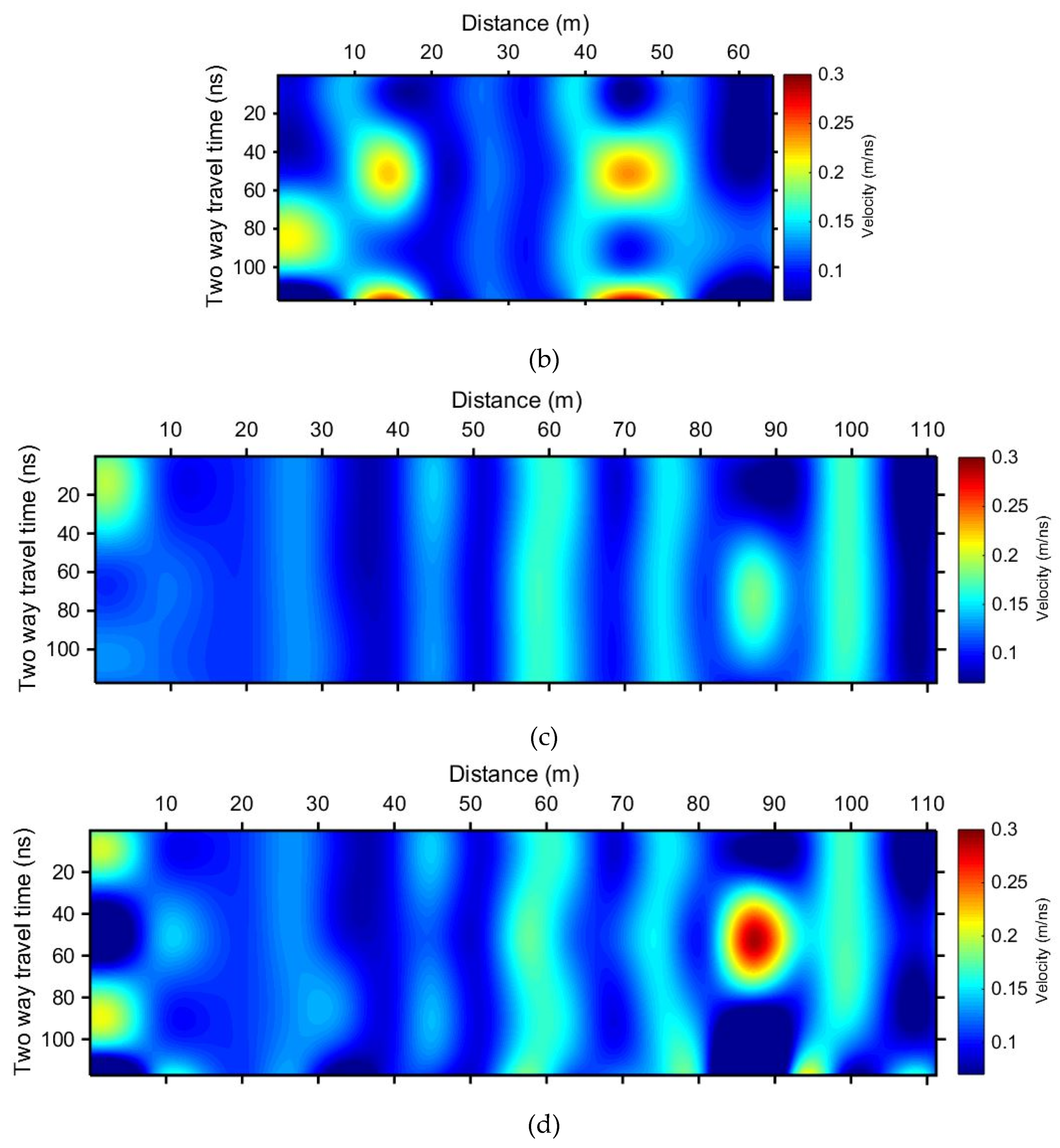
Kurtosis, k, of the data window is evaluated for each constant velocity migrated GPR section and the maximum value denotes the best focusing, thus the optimum migration velocity for the specific x-t data window. For our case, we utilized x-t windows of size x = 6 m which varied in the time direction by 20 ns. This was that the first t size was 20 ns, the second, 40 ns, the third 60 ns and so on, each one of them originating at time zero. The same implementation was used for the inline GPR sections (Figure 8a,c). Since our scope was to transform the velocity information derived in depth and x-t windows indicate a mean migration velocity within a data window, we estimated the mean interval velocities (Figure 8b,d), which were then transformed by a 1D stretch to mean interval depth velocities (Figure 9).
4. Interpretation
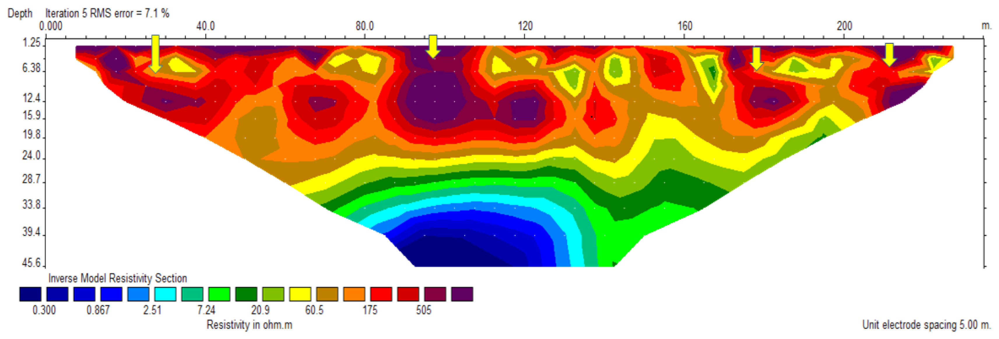
Figure 4 depicts the electrical resistivity section produced after several iterations using least square inversion. One advantage of the resistivity method is that it has helped collect data from intervals much deeper than GPR and SRT. In the resistivity tomogram, the interface between conglomerate and carbonates that is around 4 m deep is not clearly mapped. The shallow low resolution of the resistivity section is due to the 5-m electrode spacing, which was used to reach a section length sufficient for the desired section’s depth. Even though we could acquire a profile with a denser electrode interval and less prospecting depth to be combined with the former referenced ERT section, it was decided that the methodology should be tested with these parameters for a fast application of the method. This was a compromise of the shallow resolution and the total depth, as large voids and caves at relatively large depths should also be imaged. Anomalously high resistivity is observed at the cavity location (second from the left yellow arrow). This high resistivity anomaly describes the cave’s upper surface at around 7 m deep. Below this high anomaly, a very low resistive (high conductivity) zone is observed, attributed to the saltwater filling the lower part of the cavity. Above 7 m deep, the relatively high resistivity values indicate a potential low compaction zone, even though there is no surface indication for this, rather its weathered nature is visible from inside the cave’s upper surface itself. This is the only well-known ground truth of the study line.
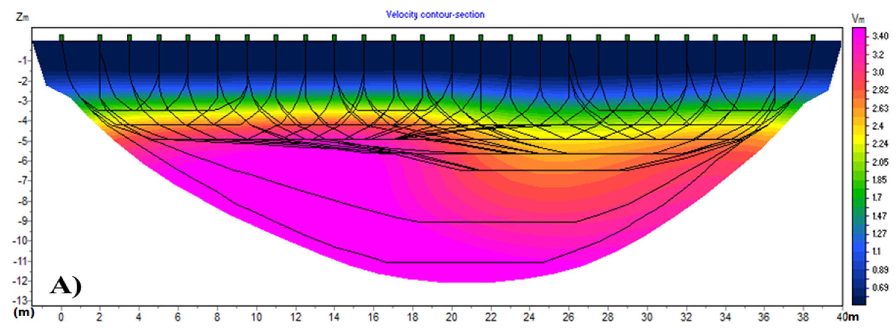
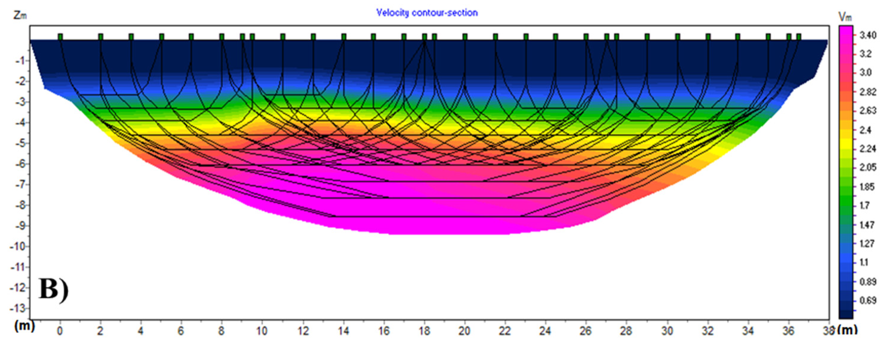
In a seismic tomographic inversion, the final model depends heavily on the characteristics of the initial velocity model. After several tests, a velocity model has been obtained and displayed in Figure 6. The observation of the inverted section inferred that the velocities vary with depth. These velocities represent the speed of seismic waves in the rocks, which is directly related to the traversed rock elastic properties. It is clear from the velocity sections that the velocity of the seismic waves in the conglomerate is much lower than in the limestone. In addition, the image shows a very clear depression in a form of a low-velocity trend above the cavity at around 22 m to 32 m (Figure 6a). Additionally, with the help of the ray tracing display mode, a low to zero ray coverage is observed at the anomaly zone, indicating a possible velocity reversal. These two signs are good indications of the karst presence, as discussed earlier. These latter features that are commonly attributed to cavities or weak zones have been reported in several theoretical and field studies. Some examples include [2,10,33,34,44]. A comparison of the seismic velocity model and the traced rays from the cavity line between the inverted model and rays from the line away from the cavity indicates that the cavity exhibits both low seismic velocity values and low coverage of rays (Figure 6b).
The GPR sections revealed the presence of two subsurface rock units, which differentiate at around 50–60 ns (Figure 7a,c). The first one is conglomerate, which is characterized by relatively low reflectivity and shows numerous diffractions caused by inner heterogeneity or fractured sand boulders. The second is a layered limestone interbedded with marl. Velocity analysis using selected diffraction’s fitting indicated velocity values for the upper formation from 0.09 m/ns to 0.15 m/ns. This large variation of velocity indicates denser to looser areas, respectively, as with the lack of moisture only air content differentiates for compaction. It is a common practice to evaluate possible large heterogeneities based on the diffraction’s density within the section. This is also known to be an unsafe approach as relatively high amplitude diffractions’ existence depends on the combination of the dominant frequency of the GPR signal, the EM velocity of the subsurface (both indicating the wavelength of the signal), and the size of the heterogeneities. To circumvent this, we based our interpretation on velocity analysis of the sections after plane wave destruction (Figure 8). We are aware that the 1D transformation to interval velocities lacks a solid theoretical base for the main reason that we do not have a laterally homogeneous medium, as depicted in Figure 8a,c. To deal with the problem of the conversion from time–migration velocities to interval velocities in depth, in the presence of lateral velocity variation, [45] utilized Dix velocities inversion involving image rays. We do not use the outcome velocity either for migration and time-to-depth conversion of the GPR section or for further estimation of other physical properties such as dielectric permittivity. Even though the latest examples in the literature followed this way [42,46], we treat our final depth velocity values in Figure 9 as an attribute, which needs calibration with other methods.
Integrated Interpretation
Even though data acquisition followed the sequence of ERT, SRT, and GPR to evaluate the first and choose the position of the latter methods, our scope is to retrieve a methodology for interpretation that follows exactly the opposite sequence.
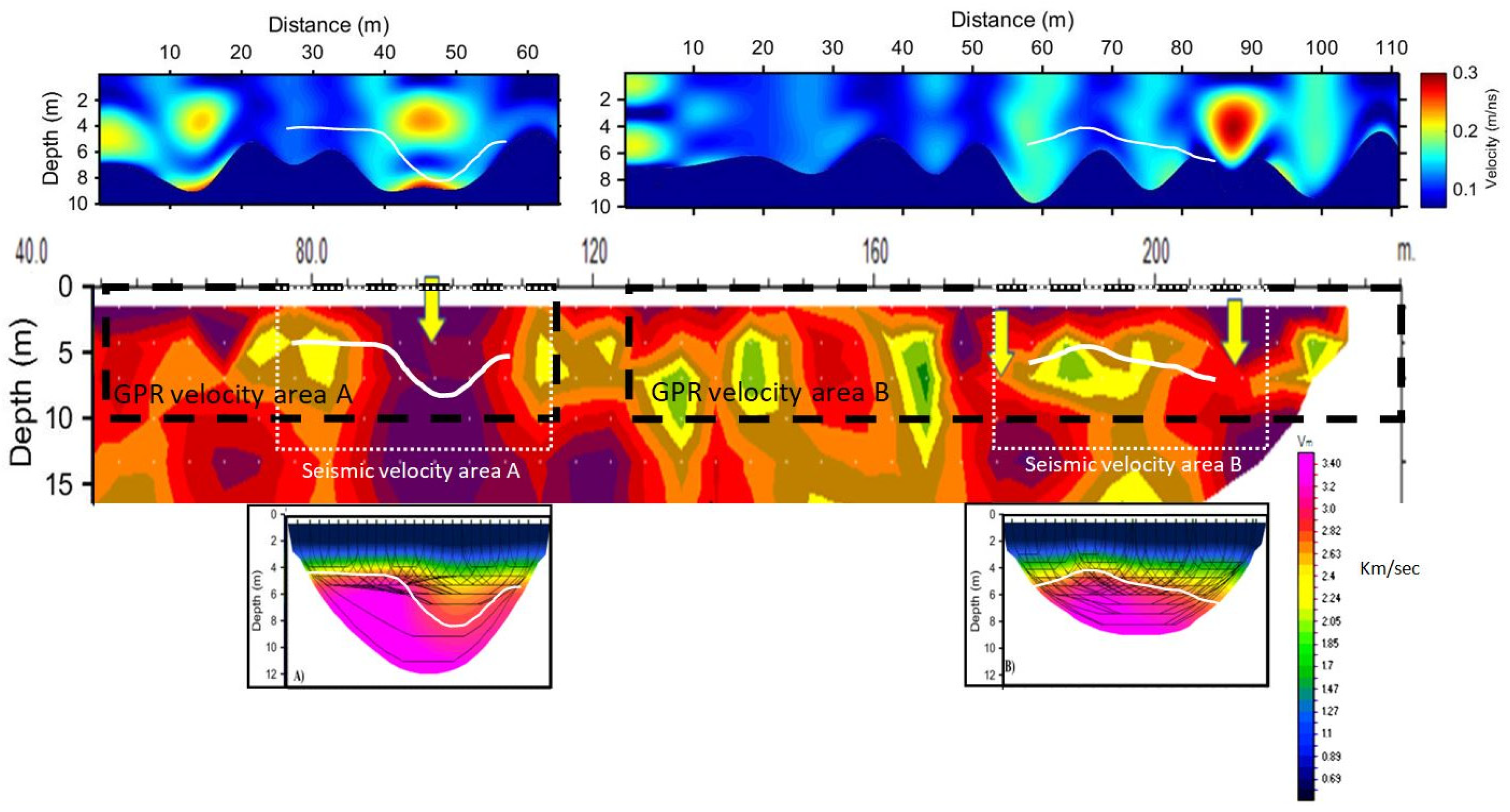
Based on the knowledge that a low compaction layer exists overlaid on a cave at a lateral position on the relevant GPR section between 40 m and 50 m, as mentioned in the seismic refraction section above, we first calibrate the high-risk zones to be described by EM velocities higher than 0.17 m/ns (Figure 10, upper left EM velocity image). This requires the study of the seismic refraction velocity models, which exhibit a dropdown of the velocity value around 2800 m/s (Figure 10, down left seismic velocity model, white line). Dropdowns in the seismic velocity coincide with GPR velocities higher than 0.17 m/ns and also with electrical resistivity values higher than 800 Ohm-m. On the other hand, seismic velocities lower than 2800 m/s coincide with areas of GPR velocities lower than 0.12–0.13 m/ns and electrical resistivity values lower than around 100 Ohm-m (Figure 10, leftmost GPR velocity image, 25–40 m lateral position, and rightmost GPR velocity image, 60–70 m lateral position). At around 80–90 m of the second GPR section (Figure 10, rightmost GPR velocity image), a very high velocity is observed, which, if this was the true EM velocity, it would be attributed to a possible void. Still, this area is just attributed to a higher risk area than the already known at the leftmost GPR velocity section, as we have already mentioned, we do not use these velocity values as a physical property but, rather, as an attribute under-calibration.
This calibration also indicates an acquisition methodology as it can be assumed to be a global parameterization for the extended area. Namely, GPR acquisition can cover all the area of interest and then adaptively estimate the same velocity attribute, which can be used for the potential high hazard zones. These zones can be further evaluated by the use of SRT, and if seismic velocity dropdowns are observed, the ERT method can be involved to image both the selected areas response and also possible origins of the weak zones at larger depths.
5. Discussion
We present a specific site dedicated methodology for detecting low compaction formations over or in carbonates. The response of the methods used here indicates that relatively large GPR velocity values, along with low seismic velocities and high electrical resistivities are attributed to subsurface parts consisting of loose sediments, prone to future surface depression. Possibly, other areas in other parts of the world could be surveyed with the scope to detect low GPR velocities and resistivity zones, as loose formations may capture moisture. This is why the involvement of seismic is useful.
The methodology we used denotes that for the specific case study and target GPR should not be used as a standalone method. Our work presents the GPR method as a valuable tool used as a pioneering method to cover a large area for dolines assessment. Hopefully, the area lacks moisture and, thus, the GPR signal penetrates at depths more than 5 m, adequate for our scope. Its response can be further evaluated by SRT and ERT methods at selected areas. Acquisition of geophysical data follows a sequence from the easiest and fastest to implement the method to the harder. This is essential due to both acquisition costs and time, but also very useful in areas like the one we present here due to extreme weather conditions. For processing, to enhance the applicability of the GPR method, we avoided diffraction analysis which is very time-consuming and suffers user’s subjectivity. The method we propose for the adaptive GPR velocity attribute estimation facilitates the GPR method’s interpretation, as long as the specific attribute is calibrated with the rest of the methods over a ground truth area.
For the time-migration velocities estimation, we use relatively large x-t windows of the section to obtain a smooth result. Each value corresponds to a mean value of the best focusing velocities of the x-t window and this makes our method have the drawback of not mapping small heterogeneities in the migration velocity values. We utilized mean time velocity values for the estimation of interval depth values of the velocity attribute, which is implemented in 1D, possibly resulting in a laterally smoother result than the true GPR velocities [45], but it showed to serve us well for the specific study.
Plane-wave destruction filtering, except from enhancing the diffractions energy, also suppresses multiple energy and air diffractions. This is due to the lower dips of the latter in comparison to the former, avoiding the estimation of erroneous larger migration velocity values than the correct ones. Another similar effect could appear due to the heterogeneities of the subsurface being not pointed diffractions in relation to the EM wavelength, as reported by [47,48]. This source of ambiguity is not yet addressed or solved in our knowledge. We avoid interpretation of the GPR sections before PWD, based on the density of diffractions, as it has been done in many cases in the literature. In our opinion, this is an unsafe approach as a relatively high amplitude diffraction’s existence depends on the combination of the dominant frequency of the GPR signal, the EM velocity of the subsurface and the size of the heterogeneities. Diffraction density could also be a drawback in our proposed application—namely, the evaluation of diffraction focusing. Still, the sections after PWD indicate a large amount of diffraction energy, for the specific study, adequate for further analysis.
A potential field of research is the application of a similar approach on dense parallel study lines GPR data, considering the diffractions as 3D phenomena. Future work will also focus on the improvement of the estimation of GPR velocities by involving 2D (or 3D) transformation of time-migration velocities to depth velocities, which, along with attenuation evaluation, can lead to dielectric permittivity values.
6. Conclusions
An integrated geophysical survey using the Ground-Penetrating Radar, Seismic Refraction Tomography, and Electrical Resistivity methods was carried out in Northern Oman to examine the ability to evaluate areas of low compaction that could potentially give surface depressions or sinkholes above a tertiary carbonate rock. This is a preliminary study, part of a larger future research, which had the scope to adopt an efficient methodology for the extended area. We estimated an adaptive GPR velocity attribute in x-t windows, based on the best focusing of the diffractions, whose values were calibrated by seismic velocities and electrical resistivity values over a ground truth area to interpret the shallow subsurface. This concluded at a specific site dedicated acquisition methodology, with the GPR method leading the way and covering all the area leaving the rest of the methods to be used as complementary and only at selected areas of great interest.
Author Contributions
Conceptualization, M.F. and N.E.; methodology, M.F. and N.E.; software, M.F. and N.E.; validation, M.F. and N.E.; formal analysis, all authors; investigation, all authors; resources, all authors; data curation, all authors; writing—original draft preparation, all authors; writing—review and editing, all authors; visualization, all authors; supervision, all authors; project administration, all authors; funding acquisition, M.F. and O.A. All authors have read and agreed to the published version of the manuscript.
Funding
This research was funded by Sultan Qaboos University, grant number IG/SCI/ETHS/19/01.
Data Availability Statement
Data available upon request.
Conflicts of Interest
The authors declare no conflict of interest.
References
- Chalikakis, K.; Plagnes, V.; Guerin, R.; Valois, R.; Bosch, F.P. Contribution of geophysical methods to karst-system exploration: An overview. Hydrogeol. J. 2011, 19, 1169–1180. [Google Scholar] [CrossRef]
- Martínez-Moreno, F.J.; Galindo-Zaldívar, J.; Pedrera, A.; Teixido, T.; Ruano, P.; Peña, J.A.; Martín-Rosales, W. Integrated geophysical methods for studying the karst system of Gruta de las Maravillas (Aracena, Southwest Spain). J. Appl. Geophys. 2014, 107, 149–162. [Google Scholar] [CrossRef]
- Wadas, S.; Polom, U.; Krawczyk, C.M. High-resolution shear-wave seismic reflection as a tool to image near-surface subrosion structures—A case study in Bad Frankenhausen, Germany. Solid Earth 2016, 7, 1491–1508. [Google Scholar] [CrossRef] [Green Version]
- Farfour, M.; Osman, A.; Al-Shukaili, F. Geophysical investigation of underground cavity in Bimmah Sinkhole, Northern Oman. In Proceedings of the Fifth International Conference on Engineering Geophysics (ICEG), Al Ain, United Arab Emirates, 21–24 October 2019; pp. 203–206. [Google Scholar]
- Parise, M.; Gabrovsek, F.; Kaufmann, G.; Ravbar, N. Recent advances in karst research: From theory to fieldwork and applications. Geol. Soc. Spec. Publ. 2018, 466, 1–24. [Google Scholar] [CrossRef]
- Loke, M.H. Tutorial: 2-D and 3-D Electrical Imaging Surveys; Geotomo Software Company: Houston, TX, USA, 2013. [Google Scholar]
- Afshar, A.; Abedi, M.; Norouzi, G.H.; Riahi, M.A. Geophysical investigation of underground water content zones using electrical resistivity tomography and ground penetrating radar: A case study in Hesarak-Karaj, Iran. Eng. Geol. 2015, 196, 183–193. [Google Scholar] [CrossRef]
- El-Kaliouby, H. GPR study of karst in a carbonate coastal area for evaluating its suitability for construction, Wadi Shab, Eastern Oman. In Proceedings of the International Conference on Engineering Geophysics 2015, Al Ain, United Arab Emirates, 15–18 November 2015. [Google Scholar]
- Mohamed, A.M.E.; El-Hussain, I.; Deif, A.; Araffa, S.A.S.; Mansour, K.; Al-Rawas, G. Integrated ground penetrating radar, electrical resistivity tomography and multichannel analysis of surface waves for detecting near-surface caverns at Duqm area, Sultanate of Oman. Near Surf. Geophys. 2019, 17, 379–401. [Google Scholar] [CrossRef]
- Senkaya, G.; Senkaya, M.; Karsli, H.; Güney, R. Integrated shallow seismic imaging of a settlement located in a historical landslide area. Bull. Eng. Geol. Environ. 2020, 79, 1781–1796. [Google Scholar] [CrossRef]
- Gan, F.; Han, K.; Lan, F.; Chen, Y.; Zhang, W. Multi-geophysical approaches to detect karst channels underground—A case study in Mengzi of Yunnan Province, China. J. Appl. Geophys. 2017, 136, 91–98. [Google Scholar] [CrossRef]
- Varnavina, A.V.; Khamzin, A.K.; Kidanu, S.T.; Anderson, N.L. Geophysical site assessment in karst terrain: A case study from southwestern Missouri. J. Appl. Geophys. 2019, 170, 103838. [Google Scholar] [CrossRef]
- Bechtel, T.D.; Bosch, F.P.; Gurk, M. Chapter Four- Geophysical methods. In Methods in Karst Hydrogeology International Contribution to Hydrogeology; Goldscheider, N., Drew, D., Eds.; Taylor and Francis: London, France, 2007; Volume 26, pp. 171–199. [Google Scholar]
- Kaufmann, G. Geophysical mapping of solution and collapse sinkholes. J. Appl. Geophys. 2014, 111, 271–288. [Google Scholar] [CrossRef]
- Margiotta, S.; Negri, S.; Parise, M.; Valloni, R. Mapping the susceptibility to sinkholes in coastal areas, based on stratigraphy, geomorphology and geophysics. Nat. Hazards 2012, 62, 657–676. [Google Scholar] [CrossRef]
- Pueyo-Anchuela, O.; Casas-Sainz, A.M.; Soriano, M.A.; Pocoví-Juan, A. A geophysical survey routine for the detection of doline areas in the surroundings of Zaragoza (NE Spain). Eng. Geol. 2010, 114, 382–396. [Google Scholar] [CrossRef]
- Hussain, Y.; Uagoda, R.; Borges, W.; Nunes, J.; Hamza, O.; Condori, C.; Aslam, K.; Dou, J.; Cárdenas-Soto, M. The Potential Use of Geophysical Methods to Identify Cavities, Sinkholes and Pathways for Water Infiltration. Water 2020, 12, 2289. [Google Scholar] [CrossRef]
- Sundararajan, N.; Raef, A.; Al-Wardi, M. Integration of micro-gravity and very low frequency (VLF-EM) data analyses to outline hazardous Cavities and low rock-strength: Coastal carbonates, Wadi Shab, Oman. In Symposium on the Application of Geophysics to Engineering and Environmental Problems 2015; SAGEEP; Curran Associates, Inc.: Austin, TX, USA, 2015. [Google Scholar]
- Moraetis, D.; Mattern, F.; Scharf, A.; Frijia, G.; Kusky, T.M.; Yuan, Y.; El-Hussain, I. Neogene to Quaternary uplift history along the passive margin of the northeastern Arabian Peninsula, eastern Al Hajar Mountains, Oman. Quat. Res. 2018, 90, 418–434. [Google Scholar] [CrossRef]
- Kusky, T.; Robinson, C.; El-Baz, F. Tertiary–Quaternary faulting and uplift in the northern Oman Hajar Mountains. J. Geol. Soc. 2005, 162, 871–888. [Google Scholar] [CrossRef] [Green Version]
- Wyns, R.; Béchennec, F.; Le Métour, J. Geological Map of Sur; Sheet NF 40-08, Scale 1: 250,000; Directorate General of Minerals, Ministry of Petroleum and Minerals: Muscat, Oman, 1992. [Google Scholar]
- Salem, H. Multi- and inter-disciplinary approaches towards understanding the sinkholes’ phenomenon in the Dead Sea Basin. Appl. Sci. 2020, 2, 667. [Google Scholar] [CrossRef] [Green Version]
- Al-Shaqsi, Y.; Humaid, R.; Abdullah, F.; Khalfan, F. The Study of the Formation of Sinkholes and Its Effect on Infrastructure and Utilities. Advanced Diploma, Higher College of Technology, Muscat, Oman, 2017. [Google Scholar]
- Reynolds, J.M. An Introduction to Applied and Environmental Geophysics, 2nd ed.; John Wiley & Sons: Hoboken, NJ, USA, 2011. [Google Scholar]
- Farooq, M.; Park, S.; Song, Y.; Kim, J.; Tariq, M.; Abraham, A. Subsurface cavity detection in a karst environment using electrical resistivity (er): A case study from yongweol-ri, South Korea. Earth Sci. Res. J. 2010, 16, 75–82. [Google Scholar]
- Cardarelli, E.; Di Filippo, G.; Tuccinardi, E. Electrical resistivity tomography to detect buried cavities in Rome: A case study. Near Surf. Geophys. 2006, 4, 387–392. [Google Scholar] [CrossRef]
- El-Qady, G.; Hafez, M.; Abdalla, M.; Ushijima, K. Imaging subsurface cavities using geoelectric tomography and ground-penetrating radar. J. Cave Karst Stud. 2005, 67, 174–181. [Google Scholar]
- Adelinet, M.; Domínguez, C.; Fortin, J.; Violette, S. Seismic-refraction field experiments on Galapagos Islands: A quantitative tool for hydrogeology. J. Appl. Geophys. 2018, 148, 139–151. [Google Scholar] [CrossRef] [Green Version]
- Martinez-Lopez, J.; Rey, J.; Duenas, J.; Hidalgo, C.; Benavente, J. Electrical tomography applied to the detection of subsurface cavities. J. Cave Karst Stud. 2013, 75, 28–37. [Google Scholar] [CrossRef]
- Loke, M.H.; Barker, R.D. Rapid least-squares inversion of apparent resistivity pseudo sections by a quasi-Newton method. Geophys. Prospect. 1996, 44, 131–152. [Google Scholar] [CrossRef]
- Loke, M.H. RES2DINV—Rapid 2D Resistivity and IP Inversion Using Least-Squares Methods, User Manual; Advanced Geosciences, Inc.: Austin, TX, USA, 1998; 66p. [Google Scholar]
- Farfour, M.; Al-Hosni, T. Mapping of near-surface formations by refraction seismic tomography: A case study from Al-Amerat, Sultanate of Oman. Arab. J. Geosci. 2020, 13, 462. [Google Scholar] [CrossRef]
- Sheehan, J.R.; Doll, W.E.; Mandell, W.A. An Evaluation of Methods and Available Software for Seismic Refraction Tomography Analysis. J. Environ. Eng. Geophys. 2005, 10, 21–34. [Google Scholar] [CrossRef] [Green Version]
- Sheehan, J.R.; Doll, W.E.; Watson, D.B.; Mandell, W.A. Application of Seismic Refraction Tomography to Karst Cavities. In Proceedings of the U.S. Geological Survey Karst Interest Group Proceedings, Rapid City, SD, USA, 12–15 September 2005. U.S. Geological Survey Scientific Investigations Report 2005-5160. [Google Scholar]
- Farfour, M.; Al-Hosni, T. Application of Seismic Refraction Tomography to Map Bedrock: A Case Study from Al-Amrat, Oman: On Significant Applications of Geophysical Methods, Advances in Science, Technology & Innovation. In Proceedings of the 1st Springer Conference of the Arabian Journal of Geosciences (CAJG-1), Sousse, Tunisia, 12–15 November 2018. [Google Scholar]
- Annan, A.P. Transmission dispersion and GPR. J. Environ. Eng. Geophys. 1996, 1, 125–136. [Google Scholar] [CrossRef]
- Fernandes, A.L.; Medeiros, W.E.; Bezerra, F.H.R.; Oliveira, J.G.; Cazarin, C.L. GPR investigation of karst guided by comparison with outcrop and unmanned aerial vehicle imagery. J. Appl. Geophys. 2015, 112, 268–278. [Google Scholar] [CrossRef]
- Tzanis, A. matGPR Release 2: A freeware MATLAB® package for the analysis & interpretation of common and single offset GPR data. FastTimes 2010, 15, 17–43. [Google Scholar]
- Claerbout, J.F. Earth Soundings Analysis: Processing Versus Inversion; Blackwell Scientific Publications, Co., Inc.: Cambridge, MA, USA, 2004. [Google Scholar]
- Economou, N.; Vafidis, A.; Bano, B.; Hamdan, H.; Ortega-Rameriz, J. Ground-penetrating radar data diffraction focusing without a velocity model. Geophysics 2020, 85, H13–H24. [Google Scholar] [CrossRef]
- Fomel, S. Applications of plane-wave destruction filters. Geophysics 2002, 67, 1946–1960. [Google Scholar] [CrossRef]
- Li, C.; Zhang, J. Velocity Analysis Using Separated Diffractions for Lunar Penetrating Radar Obtained by Yutu-2 Rover. Remote Sens. 2021, 13, 1387. [Google Scholar] [CrossRef]
- Fomel, S. Shaping regularization in geophysical estimation problems. Geophysics 2007, 72, R29–R36. [Google Scholar] [CrossRef]
- Riddle, G.; Riddle, C.; Schmitt, D. ERT and Seismic Tomography in Identifying Subsurface Cavities. Geo. Can. Work Earth 2010, 1, 1–4. [Google Scholar]
- Li, S.; Fomel, S. A robust approach to time-to-depth conversion and interval velocity estimation from time migration in the presence of lateral velocity variations. Geophys. Prospect. 2015, 63, 315–337. [Google Scholar] [CrossRef]
- Yuan, H.; Montazeri, M.; Looms, M.; Nielsen, L. Diffraction imaging of ground-penetrating radar data. Geophysics 2019, 84, H1–H12. [Google Scholar] [CrossRef]
- Novais, A.; Costa, J.; Schleicher, J. GPR velocity determination by image-wave remigration. J. Appl. Geophys. 2008, 65, 65–72. [Google Scholar] [CrossRef]
- Clair, J.; Holbrook, W.S. Measuring snow water equivalent from common-offset GPR records through migration velocity analysis. Cryosphere 2017, 11, 2997–3009. [Google Scholar] [CrossRef] [Green Version]
Figure 1.
Google map depicting the location of the survey area. North is at the top of the image. The study area is located near the shoreline. Interesting geological features and structures in bathymetry are visible.
Figure 1.
Google map depicting the location of the survey area. North is at the top of the image. The study area is located near the shoreline. Interesting geological features and structures in bathymetry are visible.

Figure 2.
A simplified geological map of northern Oman that shows major formations and structures on a regional scale, including Quriat and the study area (modified after [20]). They are composed of several major units, ranging in age from Precambrian to Miocene.
Figure 2.
A simplified geological map of northern Oman that shows major formations and structures on a regional scale, including Quriat and the study area (modified after [20]). They are composed of several major units, ranging in age from Precambrian to Miocene.

Figure 3.
Area of study and study line and electrical resistivity section. A detail of relative position of different methods can be seen in Figure 9.
Figure 3.
Area of study and study line and electrical resistivity section. A detail of relative position of different methods can be seen in Figure 9.

Figure 4.
Resistivity image obtained from the inversion of apparent resistivity. The main cavity in the center is showing very high resistivity (second yellow arrow from the left). Other high-resistivity anomalies are noticed with the rest of the yellow arrows.
Figure 4.
Resistivity image obtained from the inversion of apparent resistivity. The main cavity in the center is showing very high resistivity (second yellow arrow from the left). Other high-resistivity anomalies are noticed with the rest of the yellow arrows.

Figure 5.
Samples of the shot gathers recorded over the cavity with trace scaling for visibility reasons.
Figure 5.
Samples of the shot gathers recorded over the cavity with trace scaling for visibility reasons.

Figure 6.
Velocity model derived from the tomographic inversion of the seismic refraction data. A clear drop in velocity is observed with low coverage of rays in the section above the cavity (A). While a similar response to the former is observed in the section away from the cavity (B), the latter is not.


Figure 7.
GPR processed sections. (a) Northwestern GPR section (red line at almost in the middle of the ERT profile, Figure 3), after conventional processing, (b) is (a) after plane wave destruction filtering, (c) Southeastern GPR section (red line covering almost all the second half of the ERT profile, Figure 3), after conventional processing and (d) is (c) after plane wave destruction filtering. Details for conventional processing can be found in the paper text.

Figure 8.
GPR velocities. (a) The time migration velocity of the section depicted in Figure 7b. (b) The interval velocity attribute based on (a). (c) The time migration velocity of the section depicted in Figure 7d. (d) The interval velocity attribute based on (c).


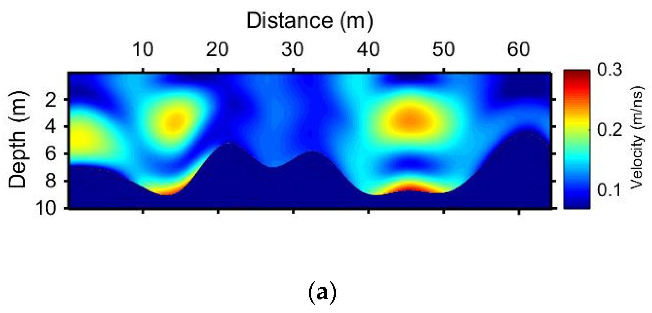
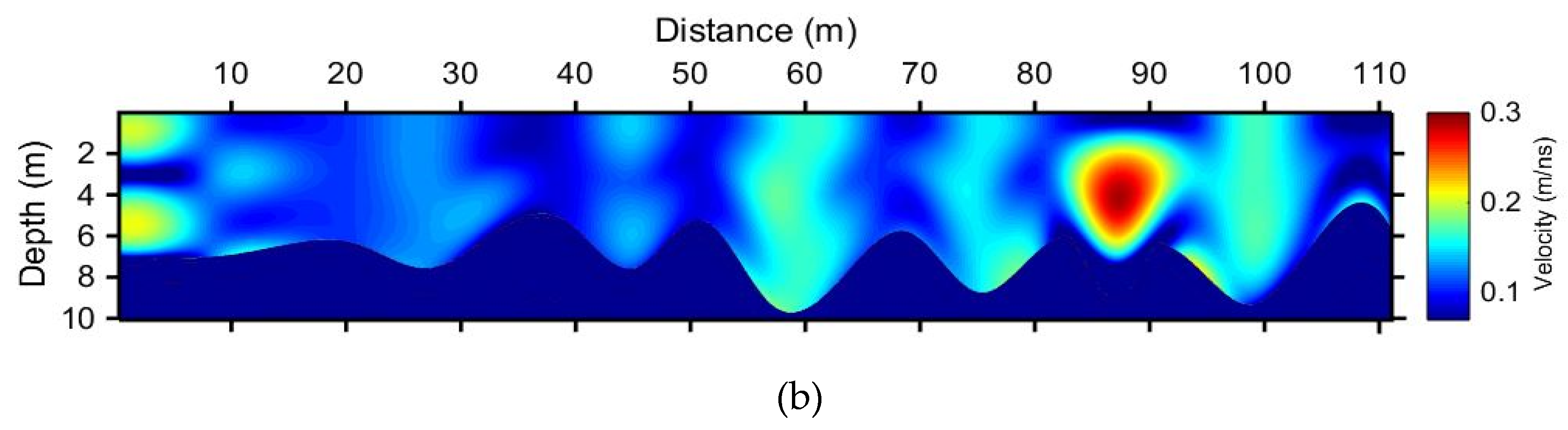
Figure 9.
GPR depth velocity attribute based (a) on time-to-depth conversion of velocities in Figure 8b and (b) in Figure 8d. Dark blue values from around 6–9 m (laterally varying) down to 10 m denote no velocity data.


Figure 10.
GPR velocity attribute calibration based on the response of the other methods over the known cave (90–105 m horizontal distance in the ERT section) and the overlaid low compaction formation (under the first yellow arrow from the left). ERT resistivity values follow the same color scale as in Figure 4. The whole image is utilized for the integrated interpretation section. White lines indicate seismic velocities around 2800 m/ns in the seismic velocity sections and are also superimposed to the other Methods sections for comparison. All other yellow arrows than the first, indicate high resistivity anomalies initially attributed to high-risk zones. All images are also depicted separately in Figure 4, Figure 6 and Figure 9.

Publisher’s Note: MDPI stays neutral with regard to jurisdictional claims in published maps and institutional affiliations. |
© 2022 by the authors. Licensee MDPI, Basel, Switzerland. This article is an open access article distributed under the terms and conditions of the Creative Commons Attribution (CC BY) license (https://creativecommons.org/licenses/by/4.0/).
Share and Cite
MDPI and ACS Style
Farfour, M.; Economou, N.; Abdalla, O.; Al-Taj, M. Integration of Geophysical Methods for Doline Hazard Assessment: A Case Study from Northern Oman. Geosciences 2022, 12, 243. https://0-doi-org.brum.beds.ac.uk/10.3390/geosciences12060243
AMA Style
Farfour M, Economou N, Abdalla O, Al-Taj M. Integration of Geophysical Methods for Doline Hazard Assessment: A Case Study from Northern Oman. Geosciences. 2022; 12(6):243. https://0-doi-org.brum.beds.ac.uk/10.3390/geosciences12060243
Chicago/Turabian StyleFarfour, Mohammed, Nikos Economou, Osman Abdalla, and Masdouq Al-Taj. 2022. "Integration of Geophysical Methods for Doline Hazard Assessment: A Case Study from Northern Oman" Geosciences 12, no. 6: 243. https://0-doi-org.brum.beds.ac.uk/10.3390/geosciences12060243
Note that from the first issue of 2016, this journal uses article numbers instead of page numbers. See further details here.