Principles of a Fast Probability-Based, Data-Adaptive Gravity Inversion Method for 3D Mass Density Modelling

Abstract

The aim of this paper is to present a 3D Probability-based Earth Density Tomography Inversion (PEDTI) method derived from the principles of the Gravity Probability Tomography (GPT). The new method follows the rationale of a previous Probability-based Electrical Resistivity Inversion (PERTI) method, which has proved to be a fast and versatile user-friendly approach. Along with PERTI, PEDTI requires no external a priori information. In this paper, after recalling the GPT imaging method, the PEDTI theory is developed and concluded with a key inversion formula that allows a wide class of equivalent solutions to be computed. Two synthetic cases are discussed to show the resolution that can be achieved in the determination of density contrasts and to examine the nature of the gravity non-uniqueness problem. Regarding the first issue, it is shown that the estimate of the density by PEDTI can change by about two orders of magnitude and get closer to reality with a more focused solution on a specific source body. Regarding the second problem, it is shown that two levels of equivalence can be classified, i.e., weak and strong equivalence, for a finer selection among the solutions. This is obtained by defining two appropriate statistical indices based on the information power of both the input and output gravity datasets.

1. Introduction

As in most geophysical methods, as well as in gravity prospecting, the inversion of field data is the most advanced step to be undertaken in order to reconstruct a physical model of the subsoil investigated. The importance of this step is clearly evident, as it constitutes a necessary path in many problems of practical nature, such as the mapping of geo-structures in tectonic and geodynamical studies, hydrocarbon, mineral and geothermal resource exploration, as well shallow-depth engineering and archaeological investigations, mainly in the reconnaissance phase of these applications.

Classically, the approach used in gravity inversion is the direct determination of the 3D distribution of density contrasts, in the subsurface, with both linear and non-linear methods [1]. Within this deterministic approach, many researchers have proposed noteworthy variants, such as, e.g., Monte Carlo simulation techniques [2], 3D inversion based on an a priori covariance model [3], and stochastic inversion techniques [4,5]. All these classical methods need to impose a priori constraints to regularize the inversion [6,7,8]. A regularization term enables them to yield a smooth or sharp model [9]. In [10,11,12], a compact and sharper image of the subsurface has been developed through a focusing method. In addition, [13,14,15,16] applied a fuzzy c-means clustering algorithm to induce the recovered physical properties to gather around clusters determined by some a priori information.

The aim of this paper is to present a new 3D data-adaptive, fast gravity inversion method, directly derived from the principles of the gravity probability tomography (GPT) [17,18]. Probability tomography, originally formulated for the self-potential method [19,20], is aimed at virtually exploring the subsoil in the search for the most probable location of the sources of the anomalies that appear in a datum domain. In gravity, a source of anomaly is a body showing a non-vanishing density contrast with respect to the reference crustal density. The GPT method is, however, intrinsically unable to give estimates of the density contrasts. In target-oriented applications, this aspect may not be a serious shortage if information on the density of the target body is not as important as its position and shape. Gravity data have been interpreted on this semi-quantitative basis in some Italian volcanic areas [21,22]. However, in many practical problems, mainly in shallow-depth investigations, information on the density value distribution in the subsoil is necessary and cannot be disregarded. To comply with this essential task and, at the same time, to take advantage of the probability tomography peculiarities, the GPT method has recently been used to provide confident geometrical constraints within a gravity full inversion program [23].

The intention is, now, to develop a fast Probability-based Earth Density Tomography Inversion (PEDTI), strictly relying on the available dataset, without requiring a priori information. The problem of equivalence (non-uniqueness) of solutions, by which gravity analysis is strongly influenced [24], is also addressed. The PEDTI method is developed following the conceptual steps previously formulated for the probability-based electrical resistivity tomography (PERTI) inversion method [25]). In this article, we will expose the idea behind the theory, as well as the application principles using relatively simple synthetic cases, which we retain enough to clarify all the key steps of the PEDTI method.

2. Outline of the GPT Theory

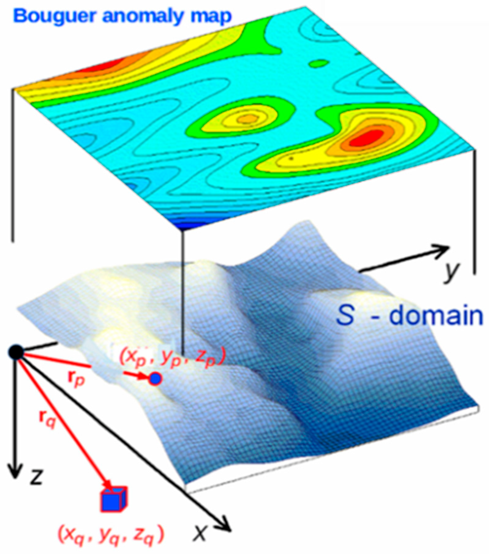
Assuming a reference system with the horizontal (x, y)-plane placed at mean sea level and the z-axis positive downwards, the gravity datum domain, generally, is a non-flat ground survey area S (S-domain in Figure 1). It is customary to plot the results of a gravity survey as a map of the Bouguer anomaly function experimentally determined at P sites r_p∈S (p = 1, 2, …, P) using the formula:

$$B_a\left(r_p\right)=g_{z,ex}\left(r_p\right)-g_{z,th}\left(r_p\right),$$

(1)

where g_z,ex(r_p) and g_z,th(r_p) are, respectively, the experimental (measured) and theoretical gravity vertical components at the same station point r_p ≡ x_pi + y_pj + z_pk.

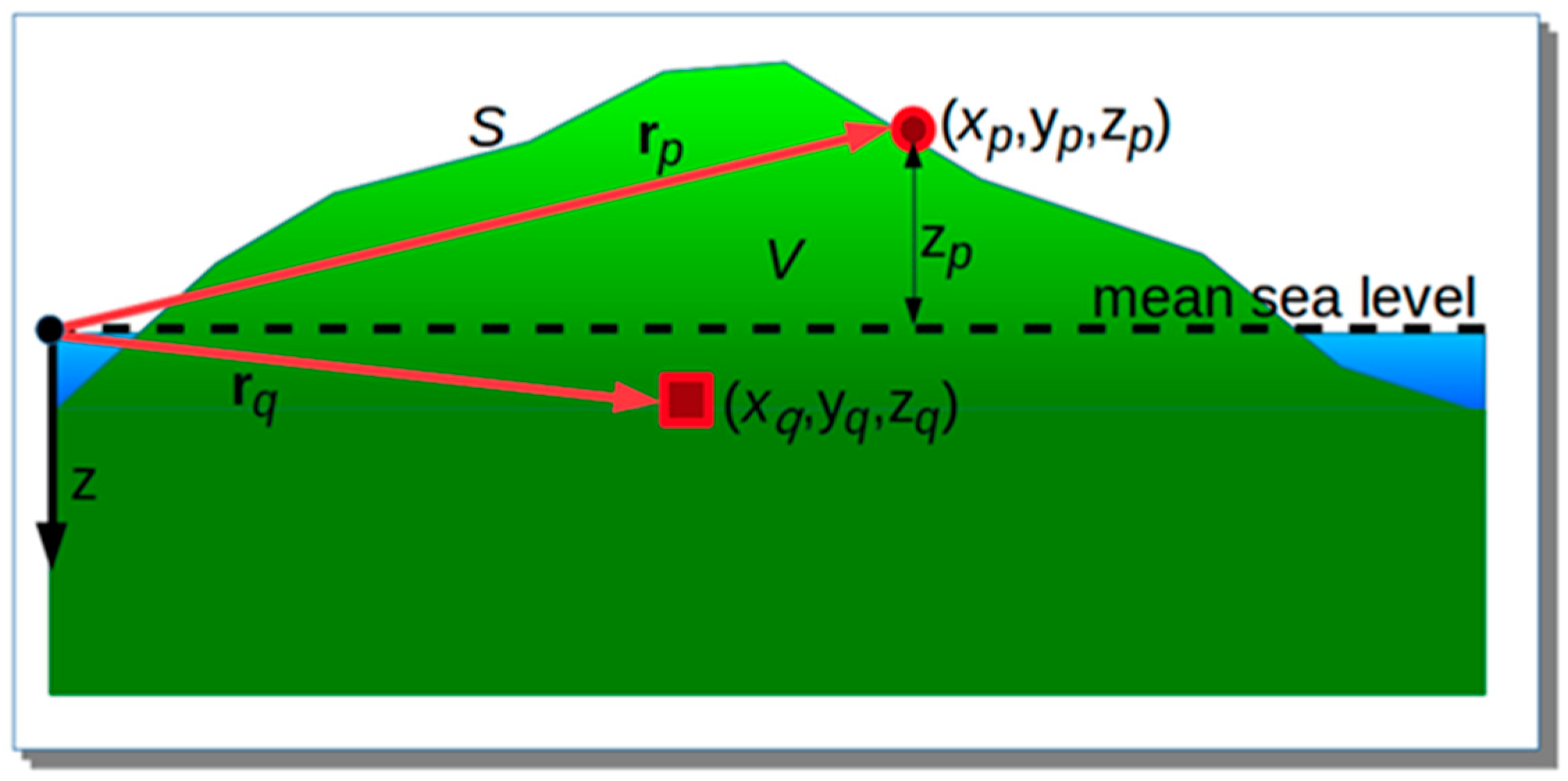
In gravity prospecting, g_z,th(r_p), either directly using the international GRS80 formula [26] or a modification of it containing free-air, plate, and terrain corrections, relies on a reference density value σ_o, generally assumed to be the average crustal density. To be more explicit, referring to the most common case of inland ground measurements, as sketched in Figure 2, the formula currently used for g_z,th(r_p) is [27]:

$$g_{z,th}\left(r_p\right)=g_o\left[1+k_{1}si{n}^2\phi \left(r_p\right)-k_{2}si{n}^{2}2\phi \left(r_p\right)\right]+{\sigma }_{o}G\left[2\pi \left|z_p\right|-T_c\left(z_p\right)\right]-k_3\left|z_p\right|,$$

(2)

where k₁ = 5.3024 × 10⁻³, k₂ = 5.8 × 10⁻⁶ and, using SI units, g_o = 9.780327 m/s², σ_o = 2670 kg/m³, G = 6.6742 × 10⁻¹¹ m³/s²kg, k₃ = 3.086 × 10⁻⁶ s⁻², with z_p in m.

In (2), the term 2πGσ_o|z_p| is the positive contribution of the slab confined between the mean sea level and the pth station level (vanishes if z_p = 0). The term −Gσ_oT_c(z_p) is, instead, the negative terrain correction, needed whenever lateral deviations from slab flatness cannot be neglected. For the calculation of T_c(z_p) Messerschmidt’s formula is used [28]. Finally, the term −k₃z_p is the negative free-air correction needed to account for the altitude of the station site above sea level (vanishes if z_p = 0).

In the original GPT formulation [17,18], the B_a(r_p) function was assumed to be of the type:

$$B_a\left(r_p\right)={{\displaystyle \sum }}_{q=1}^Q{\Gamma }_q\lambda \left(r_p,r_q\right),$$

(3)

i.e., as a sum of signals from Q elementary sources (poles), located in the subsoil in such a way as to generate an anomaly contour map such as in the top Figure 1. In (3), r_q ≡ x_qi + y_qj + z_qk is the position of the qth pole (q = 1, 2, …, Q), Γ_q is its strength equal to the gravitational constant G times the differential mass Δm_q concentrated at the centre, and λ(r_p,r_q) is the so-called scanning function [17,18], given as:

$$\lambda \left(r_p,r_q\right)=\left(z_q-z_p\right)/{\left|r_q-r_p\right|}^3.$$

(4)

Equation (3) is a convenient discretization of the most general Newtonian form:

$$B_a\left(r_p\right)={{\displaystyle \int }}_V\lambda \left(r_p,r_q\right)d{\Gamma }_q.$$

(5)

The GPT theory starts by introducing a total information power Λ, associated with B_a(r_p), given as:

$$\Lambda ={{\displaystyle \sum }}_{p=1}^P{B}_a^2\left(r_p\right).$$

(6)

Additionally, (6) is a convenient discretization derived from the most general form of signal energy in the space-domain, previously used by [17], i.e.,

$$\Lambda ={{\displaystyle \int }}_S{B}_a^2\left(r_p\right)dS.$$

(7)

Substituting from (3), (6) becomes:

$$\Lambda ={{\displaystyle \sum }}_{q=1}^Q{\Gamma }_q{{\displaystyle \sum }}_{p=1}^P{B}_a\left(r_p\right)\lambda \left(r_p,r_q\right).$$

(8)

Taking a generic qth addendum from (8) and using Cauchy–Schwarz inequality property, it follows:

$${\left[{{\displaystyle \sum }}_{p=1}^P{B}_a\left(r_p\right)\lambda \left(r_p,r_q\right)\right]}^2\le {{\displaystyle \sum }}_{p=1}^P{B}_a^2\left(r_p\right)\cdot {{\displaystyle \sum }}_{p=1}^P{\lambda }^2\left(r_p,r_q\right),$$

(9)

from which a Δm_q-occurrence probability function η(r_q), valid for 3D GPT, is at last derived as [17]:

$$\eta \left(r_q\right)=C\left(r_q\right){{\displaystyle \sum }}_{p=1}^P{B}_a\left(r_p\right)\lambda \left(r_p,r_q\right),$$

(10)

where:

$$C\left(r_q\right)={\left[{{\displaystyle \sum }}_{p=1}^P{B}_a^2\left(r_p\right)\cdot {{\displaystyle \sum }}_{p=1}^P{\lambda }^2\left(r_p,r_q\right)\right]}^{-1/2}.$$

(11)

The η(r_q) is a normalised correlation function satisfying the condition: −1 ≤ η(r_q) ≤ +1. The GPT is, therefore, a fast imaging procedure of a set of η(r_q) values, calculated at the nodes of a 3D grid (the tomospace), placed beneath the S-domain. A positive value of η(r_q) indicates a positive discrepancy of density at the point r_q, with respect to the reference density σ_o, while a negative value is the result of a negative discrepancy of density at r_q. Contouring of all the η(r_q) values allows the geometrical pattern of all the anomaly sources to be delineated. For the purposes of the PEDTI method we are going to develop, it is important to stress since now that the situation, in which η(r_q) = 0, corresponds to zero density discrepancy at r_q. This situation will be assumed, as will be seen in the next Section 3, as the nullity condition to be imposed point by point in the tomospace.

3. The 3D PEDTI Method

As stated in the introduction, the GPT method is unable to provide estimates of the true densities of the anomaly bodies. This limitation will now be overcome by the PEDTI approach. The idea underlying the PEDTI method is a straight consequence of the role given to the η(r_q) function. Namely, if at a point r_q resulted in η(r_q) = 0, then we can argue that the probability to find a positive or negative discrepancy of density, with respect to the prefixed reference crustal density σ_o, should vanish. Hence, at that point, the true density is likely to be close to σ_o. However, in general, in the presence of anomalies, η(r_q) ≠ 0 occurs in most of the points in the tomospace. Therefore, in order to let the nullity condition be applicable, we can adopt, here, the same reasoning as that used for the PERTI method in geoelectrical data inversion [25].

Therefore, the starting assumption for the PEDTI method is that the reference uniform density is no longer pre-assigned but assumed to be the unknown value σ_q that corresponds to a generic q-th cell of volume ΔV centred at r_q. Recalling the definition (3), such an assumption allows η(r_q) to be rewritten as:

$$\eta \prime \left(r_q\right)=G\mathrm{\Delta }VC\left(r_q\right){{\displaystyle \sum }}_{p=1}^P\left[{{\displaystyle \sum }}_{s=1}^Q\left({\sigma }_s-{\sigma }_q\right)\lambda \left(r_p,r_s\right)\right]\lambda \left(r_p,r_q\right),$$

(12)

where GΔV(σ_s−σ_q) = Γ_s corresponds to Γ_q appearing in (3). Applying the nullity condition to ηʹ(r_q), given that it is always C(r_q) ≠ 0, from (12) we readily obtain:

$${\sigma }_q={\sum }_{p=1}^P\left[{{\displaystyle \sum }}_{s=1}^Q{\sigma }_s\lambda \left(r_p,r_s\right)\right]\lambda \left(r_p,r_q\right)/{{\displaystyle \sum }}_{p=1}^P\left[{{\displaystyle \sum }}_{s=1}^Q\lambda \left(r_p,r_s\right)\right]\lambda \left(r_p,r_q\right).$$

(13)

Adding and subtracting the term ${{\displaystyle \sum }}_{p=1}^P\left[{{\displaystyle \sum }}_{s=1}^Q{\sigma }_o\lambda \left(r_p,r_s\right)\right]\lambda \left(r_p,r_q\right)$ at the numerator of (13), at last, we obtain:

$${\sigma }_q={\sigma }_o+\left\{{{\displaystyle \sum }}_{p=1}^P{B}_a\left(r_p\right)\lambda \left(r_p,r_q\right)/G\mathsf{\Delta }V{{\displaystyle \sum }}_{p=1}^P\left[{{\displaystyle \sum }}_{s=1}^Q\lambda \left(r_p,r_s\right)\right]\lambda \left(r_p,r_q\right)\right\}.$$

(14)

Equation (14) represents the basic formula of the PEDTI method. By changing r_q, it would be possible, at least in principle, to retrieve a density pattern point by point in the subsoil. However, we point out that, after repeated trials, it has resulted that one may incur in an overestimation of the denominator in the ratio at the right-hand side of (14), which is ascribable to the absence of weighing factors of the scanning functions λ(r_p,r_s) (s = 1, …, Q). In retrieving σ_q, the result may be an underestimation of the value to add to or subtract from σ_o, depending on the sign of the numerator in the ratio at the right-hand side of (14). Apparently, there is no direct physical hypothesis that may lead us to overcome such a potential obstacle. A possibility is to make recourse to the principles of the fuzzy logic, which, among others, appears fully compatible with the probabilistic paradigm we have adopted.

As is well known, the fuzzy logic belongs to a polyvalent logic, which is an extension of the Boolean logic [29]. It is related to the theory of blurry sets [30], within which we think we can, in general, include any geophysical field datasets. In fuzzy logic, the degree of truth of a variable may be any real number between 0 and 1 [29]. By degree of truth, we mean how true a property is, which can be, in addition to being true (=value 1) or false (=value 0) as in classical logic, partially true and partially false. Formally, this degree of truth is determined by an appropriate function assuming values between 0 and 1, endpoints included, which we identify, here, with the modulus of the occurrence probability function, i.e., |η(r_q)|. For the use we are going to make, it seems more appropriate to speak of |η(r_q)| as a function determining the degree of likeness, rather than the degree of truth.

In order to apply the nullity condition, we now propose a modification of the original B_a(r_p) function by including a set of calibration functions γ(r_p,r_q), one for each node r_q of the same 3D grid used for the calculation of η(r_q), such that:

$${{\displaystyle \sum }}_{p=1}^P\left[B_a\left(r_p\right)-{{\displaystyle \sum }}_{q=1}^Q\gamma \left(r_p,r_q\right)\right]\lambda \left(r_p,r_q\right)=0.$$

(15)

Of course, the calibration functions γ(r_p,r_q) must have the same form as that describing the gravity effect of a source pole over the S-domain, viz.:

$$\gamma \left(r_p,r_q\right)=G\left({\sigma }_q-{\sigma }_o\right)\mathrm{\Delta }V\lambda \left(r_p,r_q\right),$$

(16)

where (σ_q−σ_o) is the unknown density contrast at r_q (q = 1, …, Q). In passing, we observe that the left-hand side of (15) corresponds to something such as an objective function in optimization problems.

To comply with the fuzzy logic, we now introduce an unknown background density contrast (σ’−σ_o), common to all cells of the tomospace, such that:

$$\left({\sigma }_q-{\sigma }_o\right)=\left|\eta \left(r_q\right)\right|\left(\sigma \prime -{\sigma }_o\right),$$

(17)

which means that, for calculating at each r_q of the density contrast (σ_q−σ_o), we use the background value common to all cells in the tomospace, modulated by the degree of likeness function that corresponds to that point. Substituting (16) in (15) and using (17), an estimate of (σ’−σ_o) is readily obtained as:

$$\sigma \prime -{\sigma }_o=\left\{{{\displaystyle \sum }}_{p=1}^P{B}_a\left(r_p\right)\lambda \left(r_p,r_q\right)/G\mathsf{\Delta }V{{\displaystyle \sum }}_{p=1}^P\left[{{\displaystyle \sum }}_{q=1}^Q\left|\eta \left(r_q\right)\right|\lambda \left(r_p,r_q\right)\right]\lambda \left(r_p,r_q\right)\right\},$$

(18)

which, thanks to (17), allows the density σ_q to be derived at each r_q as:

$${\sigma }_q={\sigma }_o+\left\{\left|\eta \left(r_q\right)\right|{{\displaystyle \sum }}_{p=1}^P{B}_a\left(r_p\right)\lambda \left(r_p,r_q\right)/G\mathsf{\Delta }V{{\displaystyle \sum }}_{p=1}^P\left[{{\displaystyle \sum }}_{q=1}^Q\left|\eta \left(r_q\right)\right|\lambda \left(r_p,r_q\right)\right]\lambda \left(r_p,r_q\right)\right\}.$$

(19)

Equation (19) represents the key formula of the PEDTI method. One can soon verify that, when putting |η(r_q)| = 1, ∀q ϵ [1,Q], Equation (19) reduces to Equation (14).

In synthesis, the PEDTI approach does not need regularization based on a priori information. As known, regularization based on a priori information is usually introduced to eliminate higher frequency components in the solution, which cannot be constrained from the data. By the PEDTI approach, this problem is automatically avoided by the η-function in the modalities that are better explicated in the following.

Some further aspects are now worth addressing before discussing the resolution power of the PEDTI tool applied to a few simple synthetic cases. First, we observe that the sum of the calibration functions, γ(r_p,r_q) in (15), plays the role of reference model to compare with the observed Bouguer anomaly function B_a(r_p). Conceptually, it plays the same role of the starting model in any standard deterministic inversion. The main difference is that it is fully self-constrained, and no external information is required. This means that neither body geometries nor depth and/or density a priori values need to be imposed. Indeed, the calibration scheme adopted here only connects to the occurrence probability function, which is elaborated on its turn, as seen, exclusively using the field dataset.

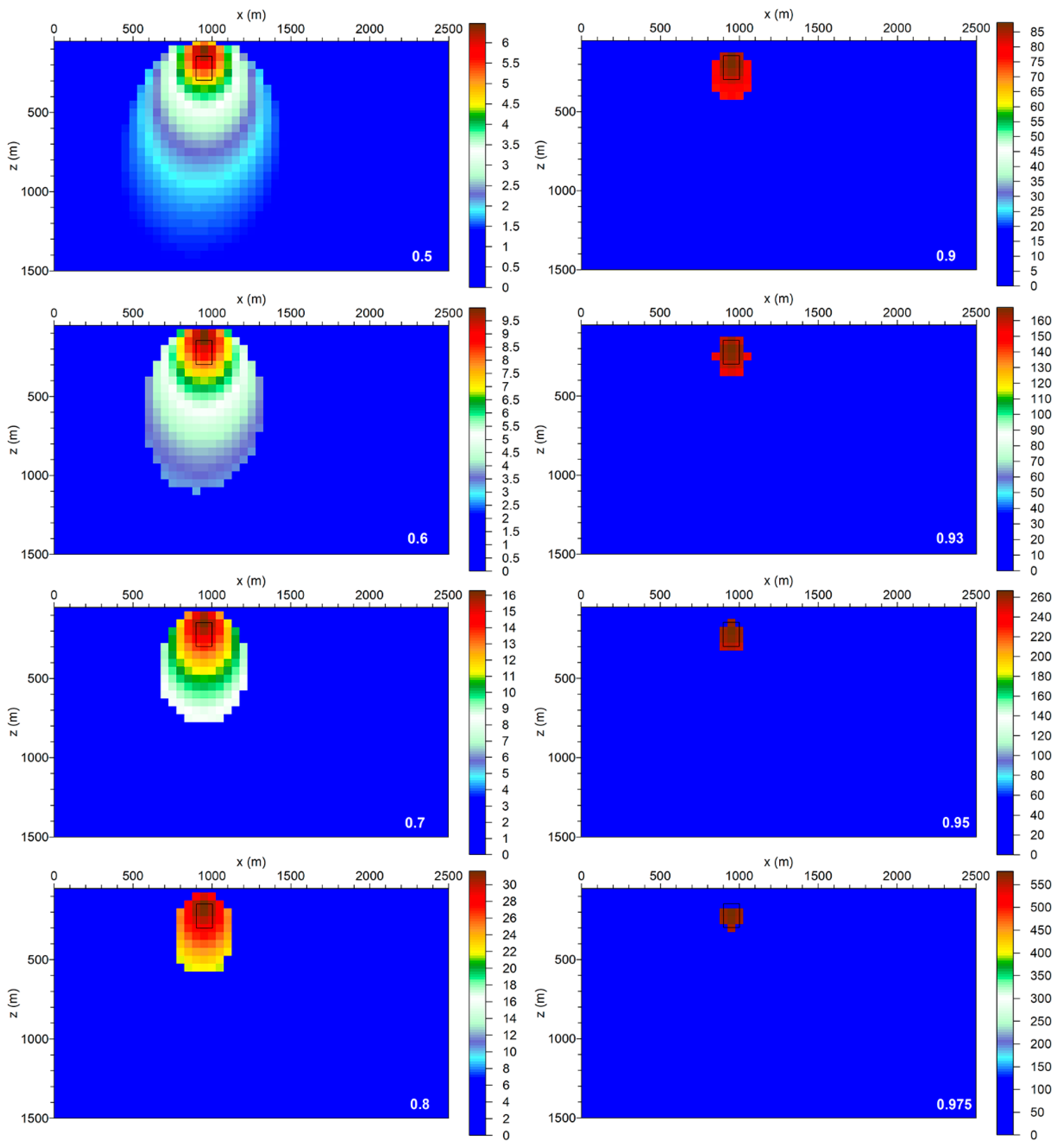
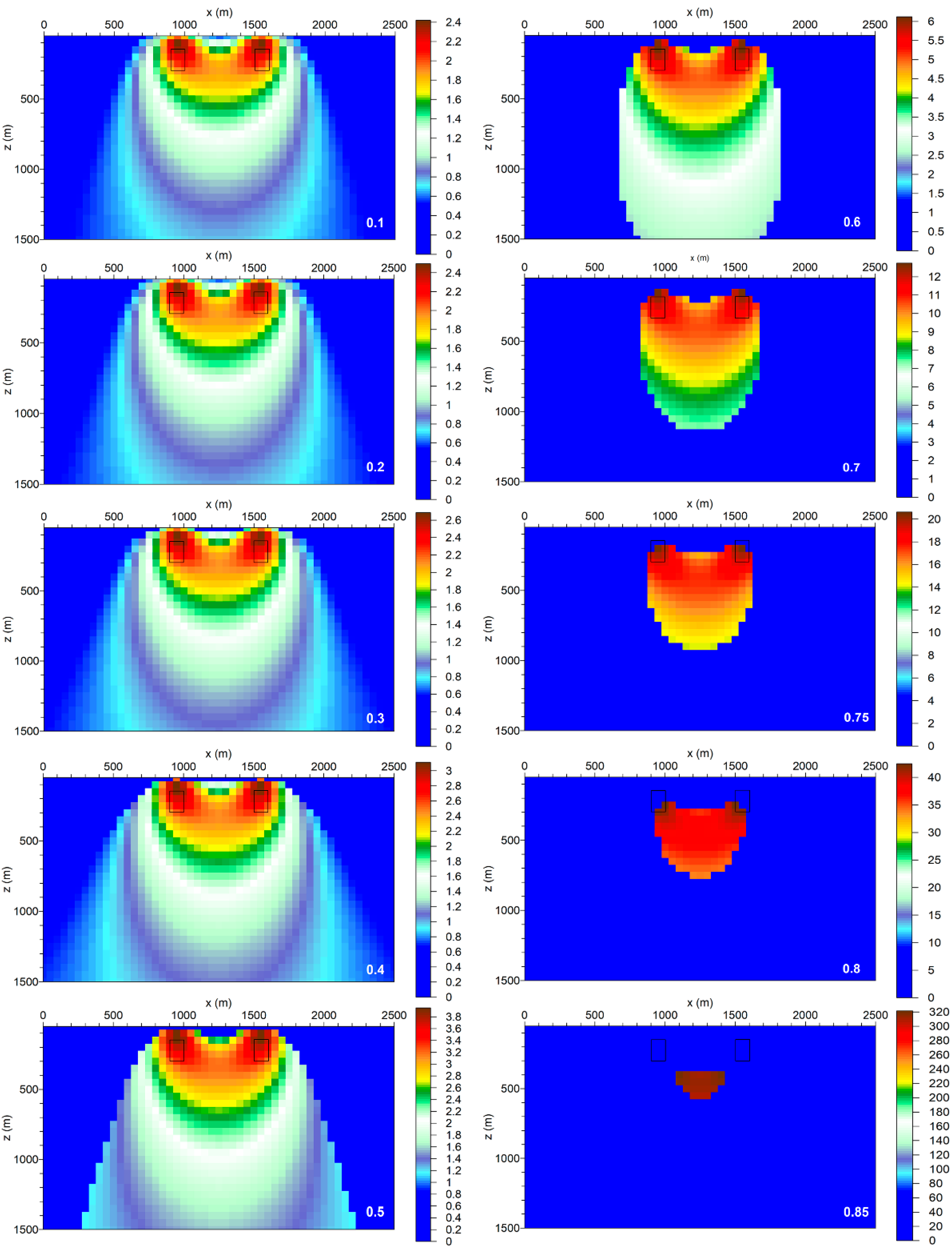
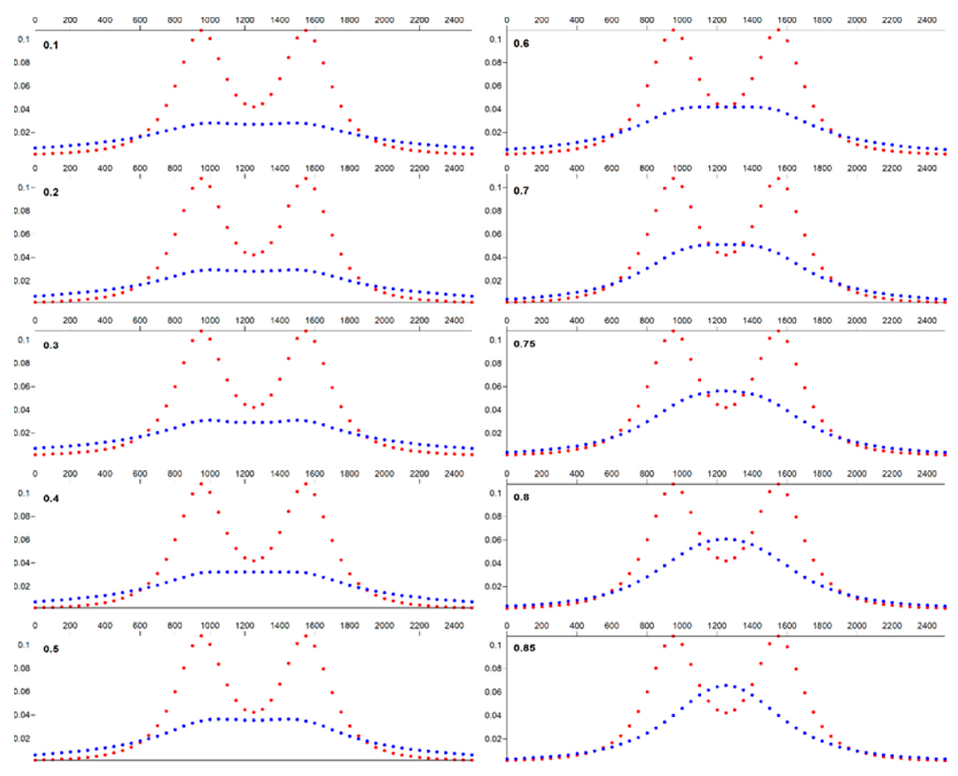
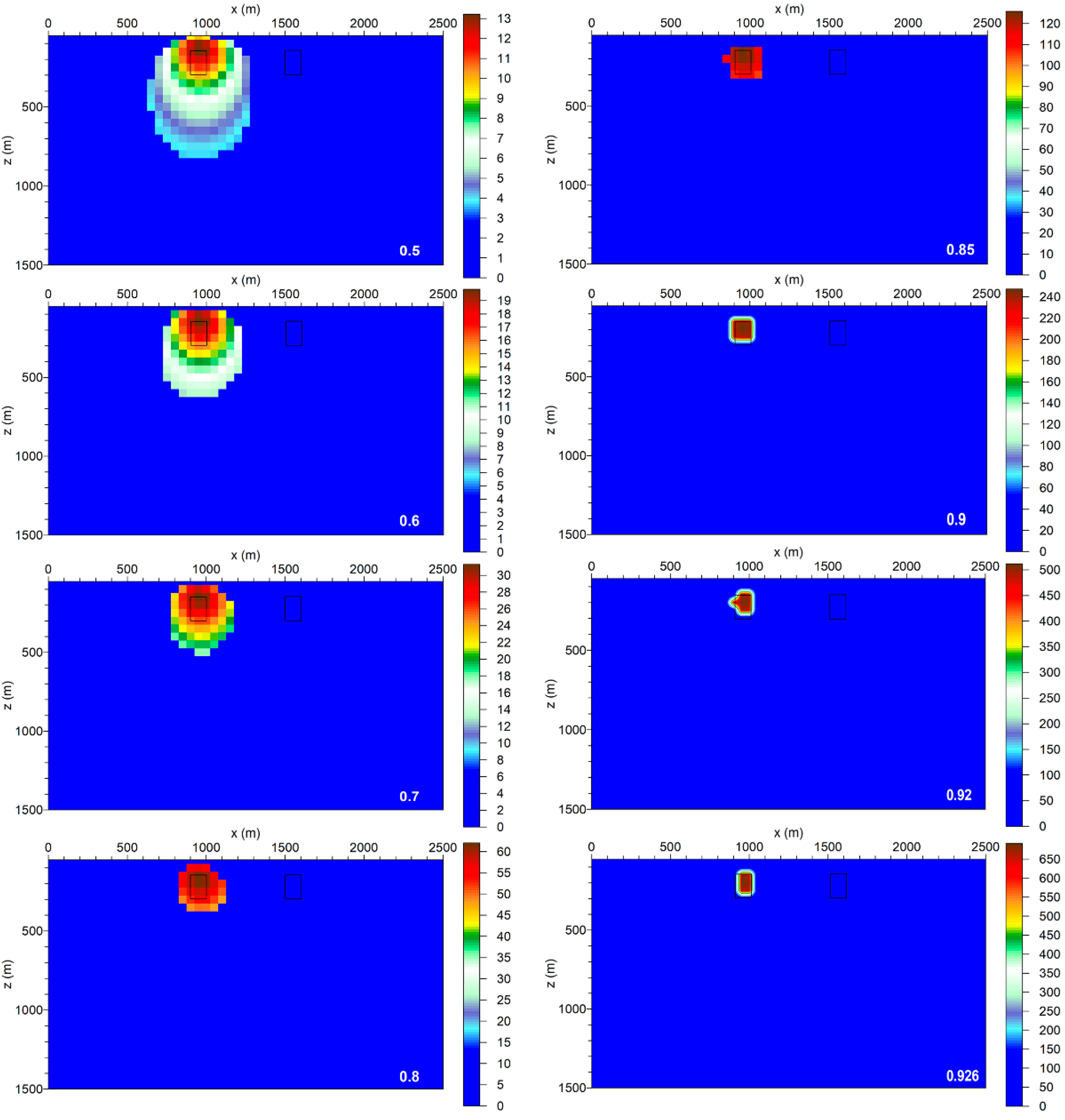
A second noteworthy aspect is how the modulus of the occurrence probability function η(r_q) acts in the estimation of the density contrast in each cell of the tomospace. We observe that |η(r_q)|, which, within the fuzzy logic we have adopted, takes the role of degree of likeness function, in Equation (19) acts in two distinct, independent ways. First, it appears as a multiplication factor of the entire ratio to the right and, therefore, through (18) brings us back to the starting position, expressed by (17), signifying the degree of likeness of the density contrast in the qth cell with the background value. Second, looking now at the inner sum at the denominator in Equation (19), |η(r_q)| appears as a weighting factor of the scanner functions, and this opens to a dynamic PEDTI approach. For instance, to better focus on areas of the tomospace enclosing peaks of the occurrence probability function, one can cut the sum by dropping out all contributions with values of |η(r_q)| lower than a prefixed threshold. Since this filtering approach can be repeated many times by increasing, at steps, the cut-off |η|-value, it can be very useful to inspect the degree of equivalence among the different solutions, as it will be shown later by the simulations.

A further important issue is the dependence of the estimate of σ_q on the volume element ΔV, which, in Equation (19), is assumed to be the same for all cells of the tomospace. The dependence of PEDTI, as well of any other inversion method on ΔV, is intrinsically unavoidable since gravity is a mass-contrast based method. The most neutral choice is assigning to ΔV the same value of the cubic voxel that is used to represent the regular grid in the 3D tomospace, whose side is the same as that of the square pixel used to represent the 2D Bouguer anomaly map. Ultimately, ΔV depends on the dataset resolution, i.e., on the amount of information it contains, according to the definition of signal power given by (6).

In conclusion, in the frame of this theory, σ_q must be intended as the density value showing the highest occurrence probability at r_q, compatible with the nature of the dataset. In synthesis, by the PEDTI approach, one searches point by point for the value that the reference density should have to allow the occurrence probability of the anomaly source to locally vanish.

4. Modelling Results and Discussion

We now show two simple synthetic cases and discuss the main features of the proposed PEDTI method. To simplify the analysis, we use Equation (19) for the situation in which the ground surface is locally flat and placed at sea level, i.e., z_p = 0, ∀p ϵ [1,P]. The two cases are the single prismatic body and the two-prism complex, all characterised by a positive density contrast with the hosting half-space.

4.1. The Single Prism Buried in a Homogeneous Half-Space

The prismatic body has square horizontal faces of 100 m sides, height of 150 m, the top surface at 150 m depth below ground level, and it is assigned a positive density contrast of 500 kg/m³. Figure 3 shows the Bouguer anomaly map generated by this prism, whose location, with respect to the reference horizontal axes, is at 900–1000 m in both the x and y directions. When processing the forward B_a(r_p) image, the portion of free surface above the source of the anomaly was divided into 2500 pixels with dimensions of 50 × 50 m². The forward B_a(r_q) dataset was obtained by a finite element program. Accordingly, Figure 4 shows the behaviour of the η(r_q) function computed with (10), applied to the whole B_a(r_p) dataset used to plot the anomaly map in Figure 3. For clarity, only a vertical section along the x-axis, through the centre of the anomaly, is depicted. The voxel unit was 50 × 50 × 50 m³, which is compatible with the resolution of the starting B_a(r_p) dataset.

Figure 5 shows the PEDTI results as a sequence of models, obtained using Equation (19), assuming, for ΔV, the same voxel unit used to draw the images in both Figure 4 and Figure 5. The scale gives the values of the density contrast in kg/m³. From left to right, the images are the result of a gradual increase in the high-pass threshold |η|-value from 0.5 up to 0.975. For example, referring to the left top section, only the points characterised by |η|-values falling in the range 0.5 ≤ |η(r_q)| ≤ 1 are included in the sum of the products |η(r_s)|λ(r_p,r_s) at the denominator of Equation (19), while points with |η(r_q)| < 0.5 are excluded, and so on, until the last cross-section (right bottom), for which the high-pass window is the narrowest one, i.e., 0.975 ≤ |η(r_q)| ≤ 1.

As for the resolution obtainable in the determination of density contrasts, the scales to the side of the sections of Figure 5 show that the estimate of the density with PEDTI can vary by about two orders of magnitude and get closer to reality the more the image is focused on the prism. Such a wide spread of density values among the PEDTI models in Figure 5 is not surprising. At least, from a qualitative point of view, we observe an inverse relationship between model size and internal density distribution: the larger the model size, the smaller the density contrasts that characterise its voxel components. Regarding this aspect, the diagrams drawn in Figure 6 are significant, where the output Bouguer anomaly profiles, generated by the reconstructed 3D PEDTI models, are compared with the input Bouguer profile generated by the prism. We, in fact, observe that the said effect can be associated with the way the input information power is redistributed by PEDTI over the survey area. Where it is observed that a substantial part of the power of the starting signal, concentrated in the peak area of the anomaly, after PEDTI is redistributed by reinforcing the weakest signals along the lateral bands, there, in parallel, is the most significant drop in the density contrast.

Figure 6 is also well suited to inspect, qualitatively, the amount of discrepancy between reconstructed and original Bouguer maps, which visibly decreases as the threshold |η|-value increases. We now place ourselves in the situation of those who have no preconceptions about the geometry and physical nature of bodies in the subsoil. Therefore, it becomes essential to be able to assess the level of equivalence of the various models recovered by PEDTI.

4.1.1. PEDTI and the Density Contrast Resolution

In gravity inversion, non-uniqueness of the solution poses unavoidable interpretation problems, due to the properties of potential fields, in that many subsurface density distributions produce equivalent responses. Following our strategy based on the use of a variable threshold |η|-value, in order to evaluate the degree of acceptance of the various solutions, we introduce two distinct equivalence levels: weak and strong equivalence levels, shortened to WEL and SEL, respectively.

The concept of WEL is associated with the ratio of the information power of the reconstructed Bouguer anomaly after inversion, i.e., B_a,r(r_p), over the information power of the observed B_a(r_p) dataset. This ratio, IPR, is directly deduced in a discretized form from (6) as:

$$IPR={{\displaystyle \sum }}_{p=1}^P{B}_{a,r}^2\left(r_p\right)/{{\displaystyle \sum }}_{p=1}^P{B}_a^2\left(r_p\right).$$

(20)

The IPR index is simply used to evaluate the level of correspondence of the whole information powers of the B_a,r(r_p) and B_a(r_p) datasets, regardless of how these powers are spread on the relative maps. Assuming that the PEDTI algorithm is, in principle, an irreversible data mining process that leads to the loss of part of the original information, we deduce that the IPR index must fit the condition 0 ≤ IPR ≤ 1. Obviously, it is always IPR ≥ 0, and IPR = 1 is the necessary condition for an ideal, lossless reversible process. Of course, the upper bound for IPR makes sense so long as no extra information is added to the dataset. If this were not the case, it would not be excluded that IPR > 1 may occur. Unfortunately, there are not yet reliable statistics allowing us to establish what the acceptance limit should be in order to fix the IPR threshold to a value above which the WEL condition is satisfied. Therefore, at this stage of our work, we are led to accept the classical 10% rule of thumb, which allows us to say that the PEDTI result that scores a 0.9 minimum IPR can safely be included within the WEL family solutions.

The concept of SEL, instead, is related to the standard model deviation, measuring the dispersion of the reconstructed Bouguer anomaly after inversion, i.e., B_a,r(r_p), from the observed one, B_a(r_p), which is normalised by the average information strength, in formula NSD (Normalised Standard model Deviation) written as:

$$NSD=\sqrt{{{\displaystyle \sum }}_{p=1}^P{\left[B_{a,r}\left(r_p\right)-B_a\left(r_p\right)\right]}^2/{{\displaystyle \sum }}_{p=1}^P{B}_a^2\left(r_p\right)}.$$

(21)

Differently from the IPR index, the NSD index is, instead, more strictly used to evaluate the point-by-point matching degree of the B_a,r(r_p) and B_a(r_p) maps. For the same reason as for the IPR index, the NSD index must also fit the condition 0 ≤ NSD ≤ 1, where it is now NSD = 0 that corresponds to the ideal, lossless reversible process. As in previous examples, we assume the 10% rule, which now allows PEDTI results that score a 0.1 maximum NSD value to be included within the SEL family solutions.

In Figure 7, the trends of the WEL and SEL indices are drawn, relative to the results depicted in Figure 5 and Figure 6. We observe that the IPR index has a moderate slope rising trend, approaching 1 and starting from about 0.6, while the NSD index has a steeper descending trend approaching 0 and starting from about 0.5. Accounting for the acceptance limits indicated above, we deduce that, at least for the single prism case, PEDTI provides a rather large set of WEL solutions, starting from a |η|-threshold slightly above 0.7, against a notably less dense set of SEL solutions, starting from a |η|-threshold slightly above 0.9.

4.2. The Two-Prism Body Buried in a Homogeneous Half-Space

We now consider a two-prism model in which both prisms have the same geometry, depth, and density contrast as those of the previous single prism case. As to the position, using the same coordinate system as before, the two prisms are aligned along the x-axis, with one prism located as it was previously and the second prism displaced at 1500–1600 m in the x direction. Figure 8 shows the Bouguer anomaly map, generated by the two-prism model, where the image resolution is the same as in the previous example. Accordingly, Figure 9 shows the corresponding behaviour of the occurrence probability function η(r_q). As noted previously, only the vertical section along the x-axis, through the centre of the twofold Bouguer anomaly, is depicted. The voxel unit was, again, 50 × 50 × 50 m³.

The two top red humps in the η(r_q) image are clearly indicative of the presence of two equiprobable bodies exactly where the two prisms are located. The most striking feature is, however, the interference phantom effect that the halos spreading from the humps produce. A deeper area is, in fact, circumscribed halfway between the two summit humps, where the highest η-values are recorded. In practice, not knowing the real nature of the causative bodies in advance, at least in principle, means the existence of a central causative body should not be excluded. This body, together with the upper lateral ones, may, indeed, constitute the nuclei of an equivalent bigger complex structure, which is equally responsible for the starting Bouguer map.

Looking now at the cross-sections in Figure 10, resulting from the application of PEDTI, a slightly different situation occurs. From the left top cross-section, we always observe an oversized complex structure, where two nuclei appear exactly in the position of the original two prisms. As in the previous example, for increasing threshold |η|-values, the tail in the models tends to gradually vanish. In this case, however, we also see a gradually increasing influence of the hypothetical body, located halfway between the two humps, in Figure 9. Until we reach the last cross-section, only this central nucleus is sharply delineated.

Moreover, we notice that the best approximation to the true value of 500 kg/m³ in both prisms is the value of 320 kg/m³, estimated within the phantom body located halfway between the two top nuclei in the depth range 375–525 m, as documented in the right bottom section in Figure 10. Hence, we are now in the presence of an apparent paradox, where the best resolved model in terms of density contrast markedly differs from the original two-prism model, which never appears so sharply delineated, and in any case, the density contrast inside the two summit nuclei reaches, at most, the value of 42 kg/m³.

As previously noted, to inspect the degree of equivalence of all these inverted models, we show, in Figure 11, the Bouguer anomaly profiles generated by them compared with that generated by the initial two-prism model. The amount of discrepancy between reconstructed and original Bouguer maps, in this case, also slightly decreases as the threshold |η|-value increases, but in all cases, it remains exceedingly high.

What helps to solve the paradox is the result expressed in Figure 12, where the trends of the IPR and NSD indices are drawn. The curve of the IPR index initially gradually increases, then flattens around its maximum value of 0.78, reached in correspondence of the |η|-threshold value of 0.75. Conversely, the curve of the NSD index initially gradually decreases, then flattens around its minimum value of 0.46, reached again in correspondence of the |η|-threshold value of 0.75. Therefore, in this case, the PEDTI method provides solutions well outside the WEL and SEL acceptance ranges.

To try to justify the discrepancies between output and input anomaly curves in Figure 11, one could argue that, mainly with the higher threshold |η|-values, the PEDTI calculated curves may represent a smoothed version of the original curve if the central ripples were misleadingly considered a noise effect. From the qualitative point of view, the PEDTI curves that would be obtained after filtering the original dataset, e.g., an upward continuation or a 2D low-pass convolution operator [31], with IPR and NSD indices falling within their respective acceptance ranges, would only exacerbate the aforementioned paradox. The result would be an enhancement of the role of the phantom body and a further reduction in the density contrast of the prisms. We do not go any further with this issue, as noise contamination in gravity is outside the scope of this paper.

After this analysis, the preliminary conclusion we arrive at is that the PEDTI method is not able to accurately resolve the coupling of two bodies when their proximity produces mutual contamination effects. By increasing the value of the |η| threshold, PEDTI shows a tendency to converge towards a solution representative of a deeper single source, which englobes the partial effects produced by all real bodies residing above it. This effect is in full agreement with what had already been outlined in a previous paper [18], where the GPT imaging, based on the source model expressed in (3), proved to be an algorithm mostly addressed to the best localization of the maximum-depth anomaly point source. We can now try to resolve this frustrating effect by making recourse to an extension of the PEDTI method, in analogy with that recently proposed for the PERTI method, labelled with the acronym E-PERTI [32,33].

E-PEDTI: An Extension of the PEDTI Method

The extension strategy is based on a peculiarity of Bernoulli’s approach in probability theory [34], which allows a multiplicity of mutually independent subsets to be extracted from the original dataset and analysed singularly. In particular, for the case under study, the subset to extract can be, for instance, the whole left hand half of the Bouguer map in Figure 8, cut in correspondence of a vertical line at 1250 m along the x axis, crossing midway through the twofold Bouguer anomaly. Hence, all the data included in the right side are excluded from further processing. The resulting occurrence probability section across the same line of 2500 m length, shown in Figure 13, is then processed by the PEDTI algorithm.

Figure 14 shows the PEDTI cross-sections corresponding to the selected data subset for a gradually increasing high-pass threshold |η|-value, from 0.5 up to 0.926. Avoiding replicating similar considerations as those previously drawn for the single prism model, at last, we see that, by this extended approach, the real left-hand side prism has now been properly reconstructed. If we consider the penultimate cross-section, which corresponds to the |η|-threshold value of 0.92, we see that the density contrast of 500 kg/m³ has been exactly recovered. If we then consider the last cross-section, which corresponds to the highest |η|-threshold value of 0.926, the density contrast exceeds the true value by as much as 30%. Of course, the same extension can be applied to the other half of the initial dataset. The corresponding analogues of Figure 13 and Figure 14 are Figure 15 and Figure 16, where one can see the vertical section of the occurrence probability function η(r_q) and the sequence of the cross-sections of the models resulting from PEDTI, respectively. At this point, we can recover the full output Bouguer anomaly profiles for the two-prism complex by adding, cell by cell, the partial Bouguer anomaly curves corresponding to the sections in Figure 14 and Figure 16. We thus obtain the sequence of curves in Figure 17, where we observe a very impressing close correspondence of the full output Bouguer anomaly profiles with the input profile, mainly starting from the |η|-threshold value of 0.8. Finally, we consider the equivalence level of this last set of E-PEDTI solutions by analysing, once again, the trends of the IPR and NSD indices shown in Figure 18. We observe that the IPR index is constantly above 0.9, while the NSD index falls below 0.1, starting from a |η|-threshold value of about 0.75. Hence, the WEL and SEL acceptance conditions are largely fulfilled.

However, there is an aspect that deserves to be commented on. It has to do with the fact that many of the IPR values are slightly greater than 1—about 4%, at most. According to the definition of IPR given in Section 4.1.1, we must admit that the practice of extending the PEDTI method to data subsets indirectly adds an amount of extra information, which leads to a surplus of information power to the numerator of (20), which defines the IPR index. Ultimately, this means that the simple summation process of the partial results, deduced by PEDTI—by means of Equation (19)—on subsets of data, does not satisfy the principle of superposition of effects, which is valid for potential fields, as demonstrated in Appendix A. Theoretically, it would satisfy it only if PEDTI’s Equation (14) were used.

However, applying the 10% rule of thumb again, if 1 < IPR ≤ 1.1, we feel we can state that the said summation process satisfies a quasi-superposition principle. The essential reason for this statement lies in the fact that all IPR values between 1 and 1.1 correspond to |η|-threshold values very close to 1. Within this extra range of IPR values, the non-linearity in Equation (19) is so weak that the superposition of results is practically not harmful. We can, therefore, consider E-PEDTI as a useful approach to solving more complex structural situations, and it is worth further investigation.

5. A Comparison between PEDTI and Classical Inversion

As documented in the previous sections, the PEDTI approach is a completely innovative gravity data inversion tool, which cannot be framed in the category of the classical deterministic inversion. It is worth recalling that, within this category, inversion is, in principle, an ill-posed problem, and regularization techniques must be introduced to try to overcome the non-uniqueness and ill-posedness obstacle [35]. PEDTI, instead, is based on theoretical and logical assumptions that differ radically from those of the classical inversion. Most important of all, the PEDTI method does not require a priori information, or pre-packaged starting models, in order to work. This property makes it completely extraneous to the risk of any subjective presetting of the model on which the solution of the inversion must converge. The synthetic examples, discussed in Section 4, showed that PEDTI is a stable inversion algorithm just because it does not require external assumptions to be regularized, nor does it need to be reformulated for numerical treatment.

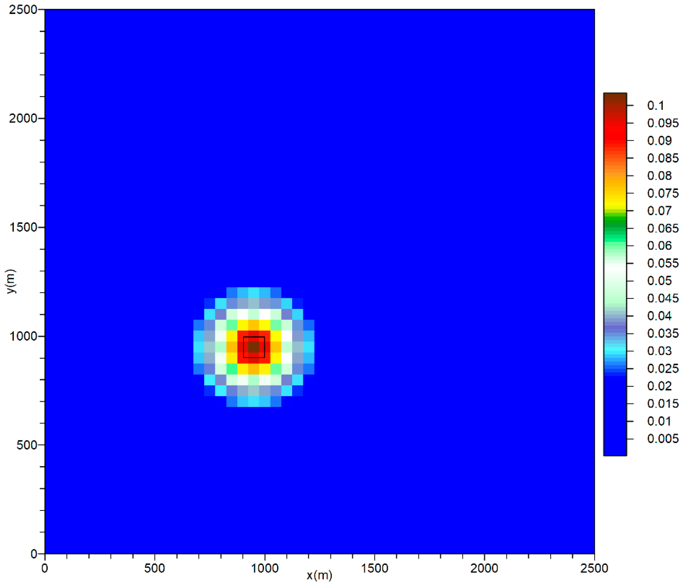
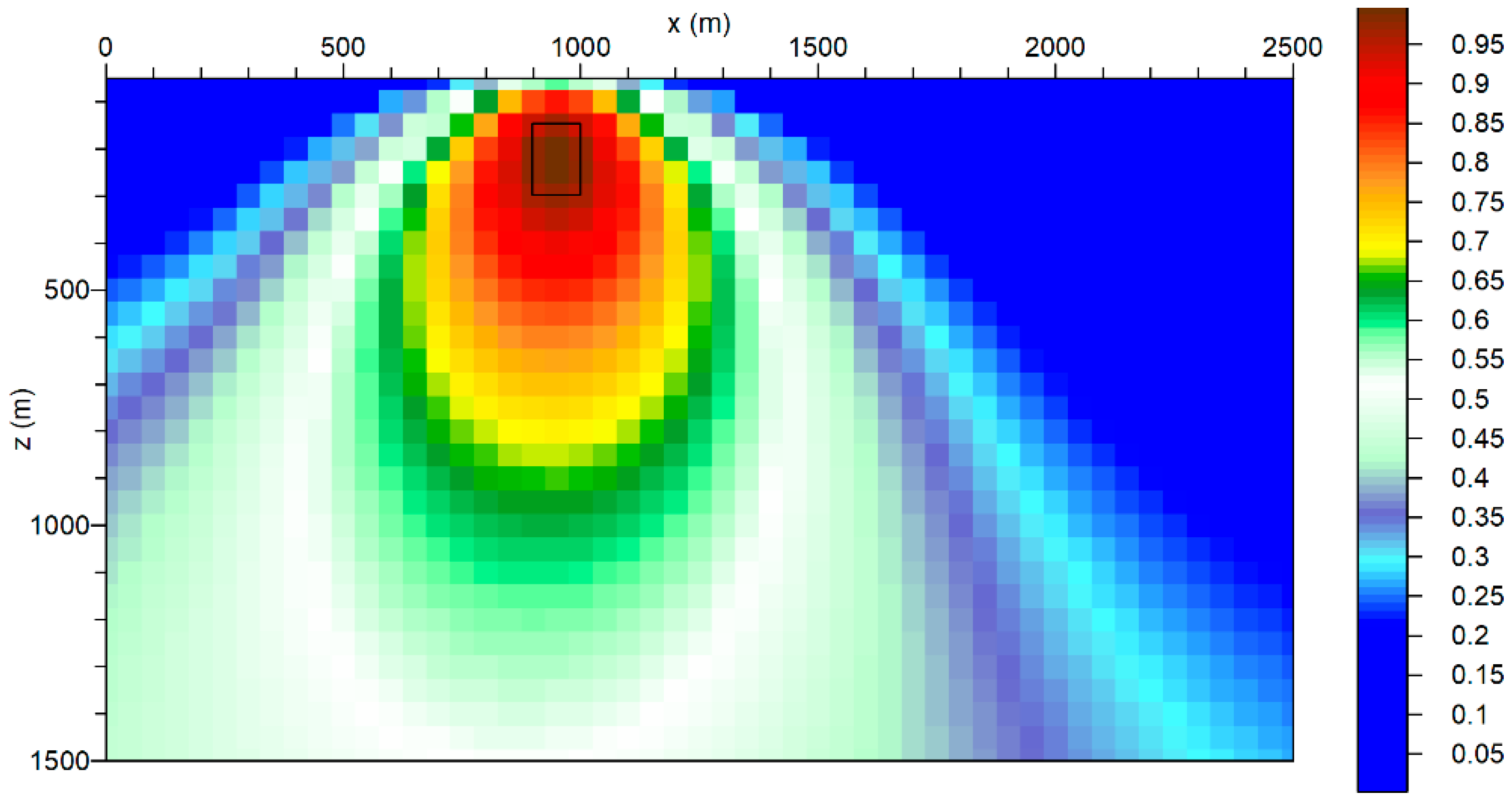
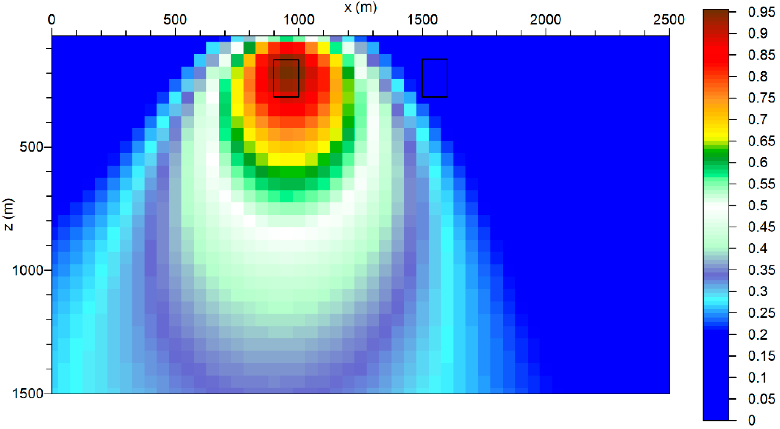
That said, it is now worth exposing a quick comparison, between our PEDTI approach and a classical deterministic inversion, in order to allow the reader to start to appreciate the benefits that PEDTI can offer. For this purpose, we consider the single prism model discussed in Section 4.1 and the relative forward Bouguer anomaly map depicted in Figure 3. For the comparison, the open source SimPEG software, in python programming language, was chosen (https://github.com/simpeg/simpeg, accessed on 31 May 2022). To put the SimPEG method in the same starting condition as PEDTI, we supposed we had no a priori information about the nature of the target body. Therefore, as a starting model to trigger the convergence of SimPEG, we assumed a homogeneous and isotropic half-space.

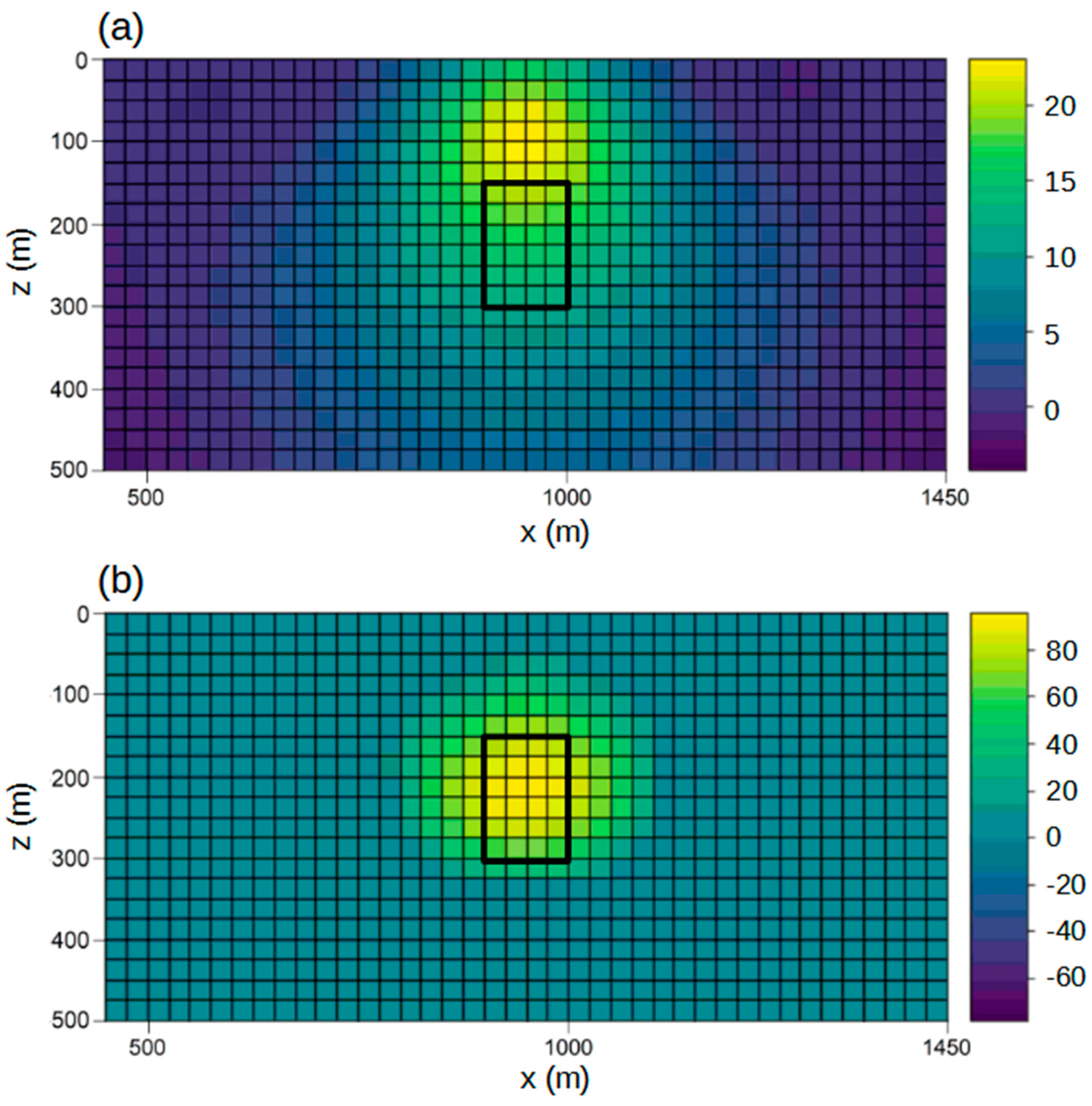
Figure 19a shows the 3D L₂-norm SimPEG inversion, across a line parallel to the x-axis, through the centre of the anomaly. Figure 19b shows a different processing with the same software by using a sparse L₂-norm regularization. Both SimPEG results are characterized by a low mismatch between the reconstructed and initial Bouguer anomaly maps. The solution in Figure 19b appears to be the one that best represents the assigned prismatic body. Comparing this last classical inversion with our best focused PEDTI result in Figure 3, we see that there is a noticeable difference in the target body density estimate. While the PEDTI density estimate is very close to the real value, the density value estimated by the SimPEG tool is about half an order of magnitude less than the real value. Moreover, we observe that, while PEDTI provides a very sharp shape of the prism, the one provided by SimPEG appears afflicted by a not negligible halo spreading all around the prism, i.e., by a blurred boundary, which can cause a difficulty in subsequent geologic interpretation [35].

Of course, we do not want to give a universal character to the conclusions reached here with only the simple example dealt with. More complex cases and comparisons with other different deterministic inversion tools would be necessary. They would, however, require a much more articulated treatment, which cannot find space in this paper, essentially dedicated to the exposition of the theoretical principles of the PEDTI method.

6. Summary and Conclusions

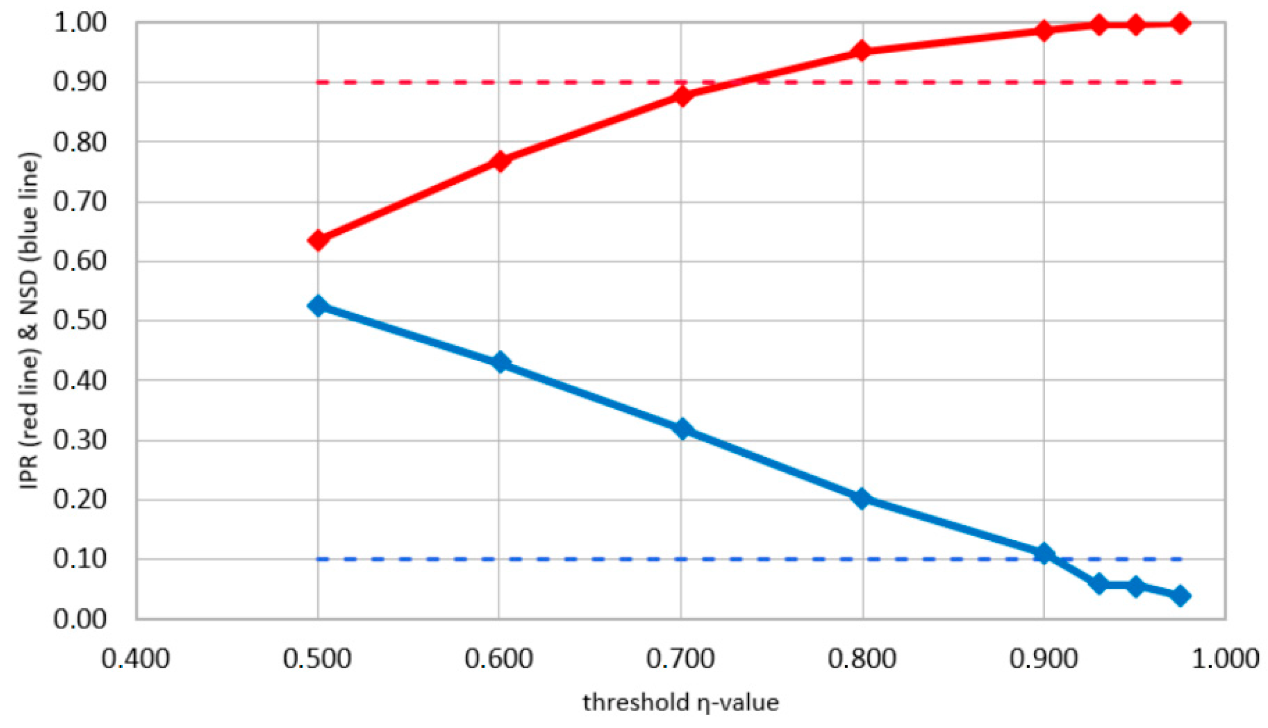
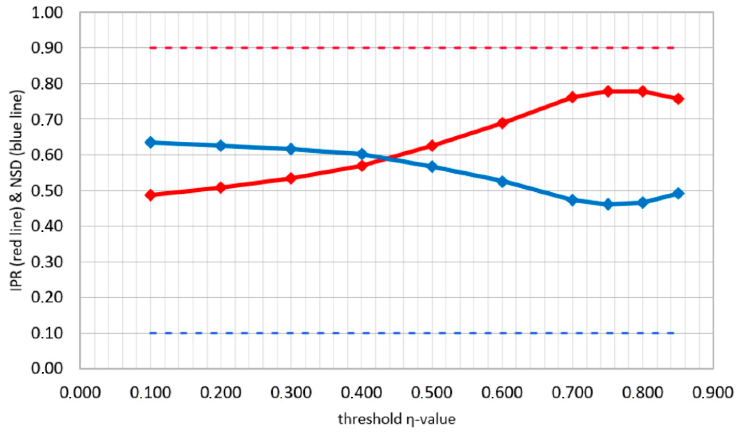
We have proposed an easy and fast 3D gravity inversion algorithm, PEDTI (Probability-based Earth Density Tomographic Inversion), which is a straight derivation from the 3D probability gravity tomography imaging theory. The PEDTI theory has been developed following the rationale previously adopted for the solution of an analogous inversion method applied to geoelectrical datasets. It consists of posing a nullity condition to the occurrence probability function, in order to retrieve the distribution of the density contrast in a 3D grid of cells, filling the investigated subsoil. To make the inversion formula fully data-adaptive, following the principles of the fuzzy logic, the occurrence probability values in the cells have been introduced as weighting factors of a set of kernel functions, which are used to calibrate, in each cell, the contributions coming from all the other cells. Using synthetic models, it has been shown that, by an iterated selection of increasingly narrow ranges of the occurrence probability weighting factors, a wide class of equivalent model solutions can be reconstructed with an increasing focusing capacity. In parallel, the gravity non-uniqueness problem has been investigated by defining two appropriate statistical indices based on the information power of both the input and output gravity datasets. It must be stressed that our PEDTI approach is not finalized to single out the model that matches with the real bodies in the subsoil. It simply aims at retrieving, from a probabilistic point of view, a class of equivalent models, opportunely constrained by the WEL and SEL indices, all compatible with the available dataset.

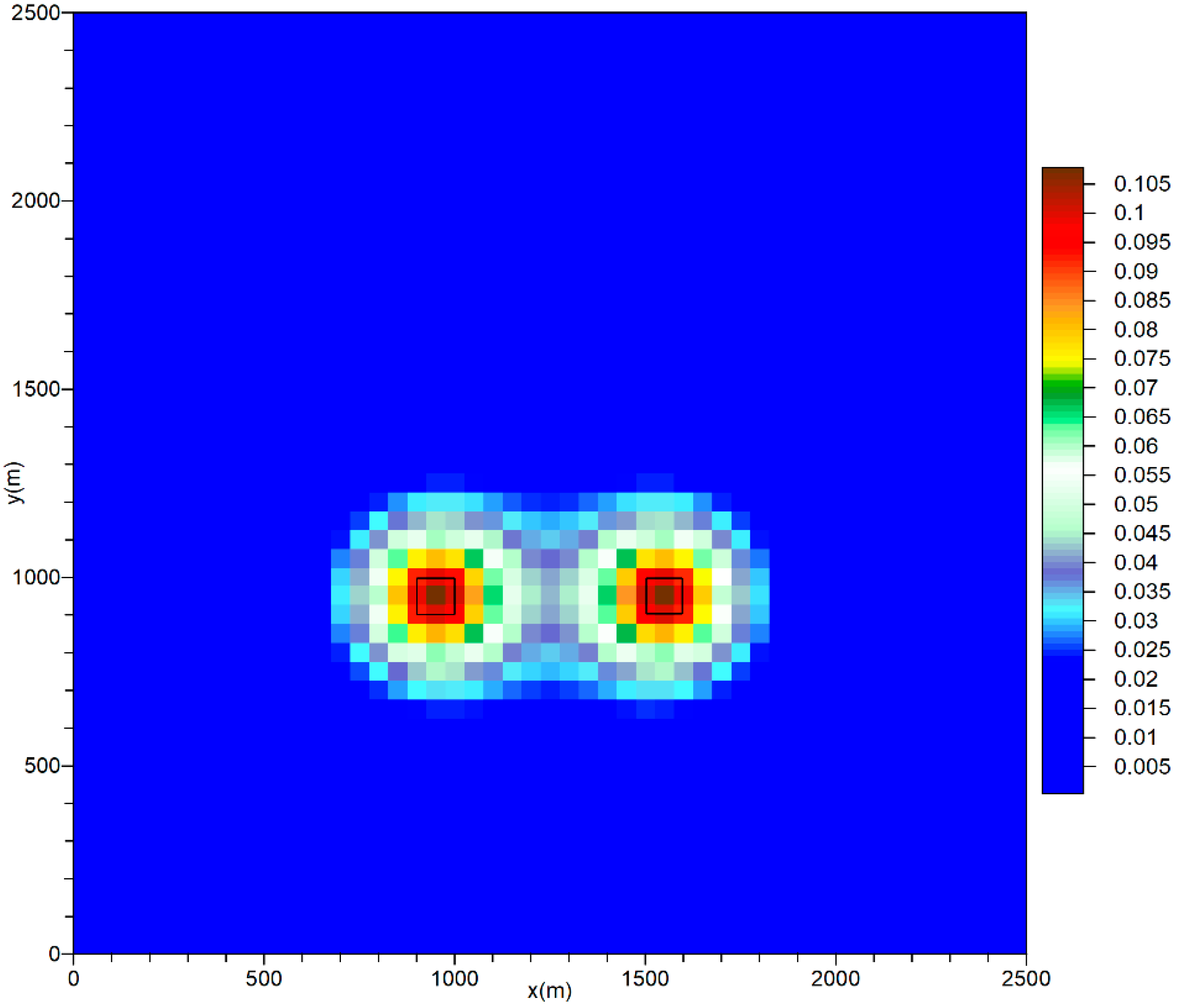
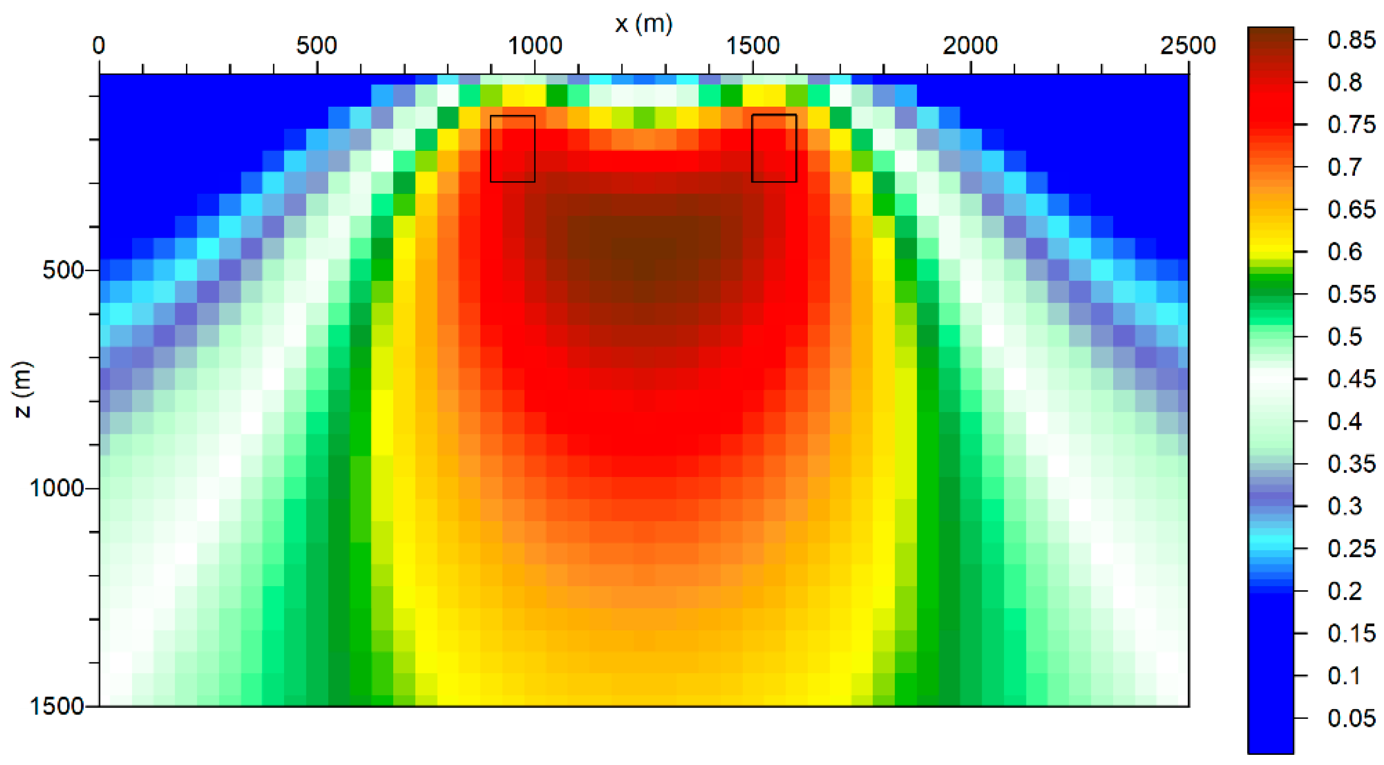
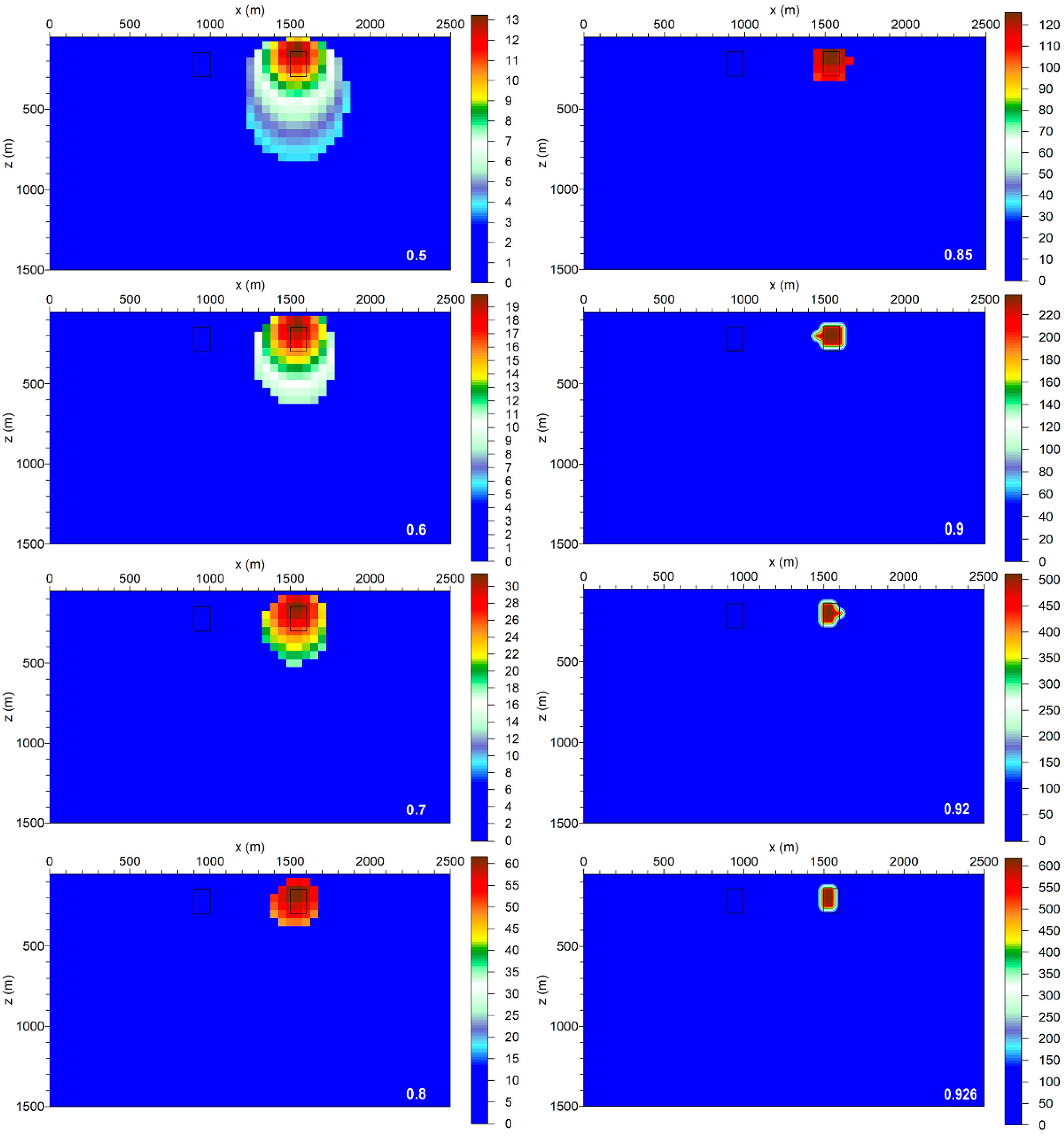
An extension of the PEDTI method, called E-PEDTI, has been introduced with the aim of addressing the problem of mutual contamination deriving from nearby sources of anomalies. Due to the complexity of this problem, we have limited our analysis to a simple symmetrical arrangement of two adjacent identical bodies. An in-depth discussion, also using bodies with different geometry and asymmetric distribution, needs a separate treatment along the lines of what we already did with the E-PERTI method in geoelectrics.

At last, it is worth pointing out that the computation time required by the PEDTI method, including the E-PEDTI extension, is very fast. For the examples we have shown in this paper, we used a laptop with a Processor Intel Core i7-12700K 3.60GHz 25M Alder Lake-S. The net computation time of the entire package, from the GPT analysis to the η-thresholding imaging, for the more complex case of the two-prism model did not exceed 2 min.

To conclude, the main features of the PEDTI method are: (i) a priori information is not a necessity; (ii) full, unconstrained adaptability to any kind of dataset, including the case of non-flat topography; (iii) fast automatic data processing and inversion using standard PCs; (iv) real-time inversion during field work, thus allowing for fast modifications of the survey plan to better focus the expected targets; (v) full independence from data acquisition techniques and spatial regularity.

References

1. Li, Y.; Oldenburg, D.W. 3-D inversion of Gravity Data. Geophysics 1998, 63, 109–119. [Google Scholar] [CrossRef]
2. Bosch, M.; McCaughey, J. Joint inversion of gravity and magnetic data under lithologic constrains. Lead. Edge 2001, 20, 877–881. [Google Scholar] [CrossRef]
3. Chasseriau, P.; Chouteau, M. 3D gravity inversion using a model of parameter covariance. J. Appl. Geophys. 2003, 52, 59–74. [Google Scholar] [CrossRef]
4. Shamsipour, P.; Marcotte, D.; Chouteau, M.; Keating, P. 3D stochastic inversion of gravity data using cokriging and cosimulation. Geophysics 2010, 75, I1–I10. [Google Scholar] [CrossRef]
5. Shamsipour, P.; Marcotte, D.; Chouteau, M.; Rivest, M.; Bouchedda, A. 3D stochastic gravity inversion using non-stationary covariances. Geophysics 2013, 78, G15–G24. [Google Scholar] [CrossRef]
6. Boulanger, O.; Chouteau, M. Constraints in 3D gravity inversion. Geophys. Prospect. 2001, 49, 265–280. [Google Scholar] [CrossRef]
7. Bosch, M.; Meza, R.; Jiménez, R.; Hönig, A. Joint gravity and magnetic inversion in 3D using Monte Carlo methods. Geophysics 2006, 71, G153–G156. [Google Scholar] [CrossRef]
8. Fullagar, P.K.; Pears, G.A.; McMonnies, B. Constrained inversion of geologic surfaces—Pushing the boundaries. Lead. Edge 2008, 27, 98–105. [Google Scholar] [CrossRef]
9. Tikhonov, A.N.; Arsenin, V.Y. Solutions of Ill-Posed Problems; Wiley: New York, NY, USA, 1977; ISBN 978-0-470-99124-4. [Google Scholar]
10. Zhdanov, M.S.; Ellis, R.; Mukherjee, S. Three-dimensional regularized focusing inversion of gravity gradient tensor component data. Geophysics 2004, 69, 925–937. [Google Scholar] [CrossRef]
11. Last, B.J.; Kubik, K. Compact gravity inversion. Geophysics 1983, 48, 713–721. [Google Scholar] [CrossRef]
12. Portniaguine, O.; Zhdanov, M.S. 3-D magnetic inversion with data compression and image focusing. Geophysics 2002, 67, 1532–1541. [Google Scholar] [CrossRef]
13. Lelièvre, P.G.; Farquharson, C.G.; Hurich, C.A. Joint inversion of seismic traveltimes and gravity data on unstructured grids with application to mineral exploration. Geophysics 2012, 77, K1–K15. [Google Scholar] [CrossRef]
14. Sun, J.; Li, Y. Multidomain petrophysically constrained inversion and geology differentiation using guided fuzzy c-means clustering. Geophysics 2015, 80, ID1–ID18. [Google Scholar] [CrossRef]
15. Sun, J.; Li, Y. Joint inversion of multiple geophysical data using guided fuzzy c-means clustering. Geophysics 2016, 81, ID37–ID57. [Google Scholar] [CrossRef]
16. Singh, A.; Sharma, S. Modified Zonal Cooperative Inversion of Gravity Data—A Case Study from Uranium Mineralization; SEG Technical Program Expanded Abstracts: Houston, TX, USA, 2017; pp. 1744–1749. [Google Scholar] [CrossRef]
17. Mauriello, P.; Patella, D. Gravity probability tomography: A new tool for buried mass distribution imaging. Geophys. Prospect. 2001, 49, 1–12. [Google Scholar] [CrossRef]
18. Mauriello, P.; Patella, D. Localization of maximum-depth gravity anomaly sources by a distribution of equivalent point masses. Geophysics 2001, 66, 1431–1437. [Google Scholar] [CrossRef]
19. Patella, D. Introduction to ground surface self-potential tomography. Geophys. Prospect. 1997, 45, 653–681. [Google Scholar] [CrossRef]
20. Patella, D. Self-potential global tomography including topographic effects. Geophys. Prospect. 1997, 45, 843–863. [Google Scholar] [CrossRef]
21. Iuliano, T.; Mauriello, P.; Patella, D. Looking inside Mount Vesuvius by potential fields integrated geophysical tomographies. J. Volcanol. Geoth. Res. 2002, 113, 363–378. [Google Scholar] [CrossRef]
22. Mauriello, P.; Patella, D.; Petrillo, Z.; Siniscalchi, A.; Iuliano, T.; Del Negro, C. A geophysical study of the Mount Etna volcanic area. In Mt. Etna: Volcano Laboratory; Geophysical Monograph, Series; Bonaccorso, A., Calvari, S., Coltelli, M., Del Negro, C., Falsaperla, S., Eds.; American Geophysical Union: Washington, DC, USA, 2004; Volume 143, pp. 273–291. ISBN 0-87590-408-4. [Google Scholar]
23. Liu, G.; Yan, H.; Meng, X.; Chen, Z. An extension of gravity probability tomography imaging. J. Appl. Geophys. 2014, 102, 62–67. [Google Scholar] [CrossRef]
24. Parasnis, D.S. Principles of Applied Geophysics; Chapman & Hall: London, UK, 1997; ISBN 978-0-412-80250-8. [Google Scholar]
25. Mauriello, P.; Patella, D. A data-adaptive probability-based fast ERT inversion method. Progr. Electromagn. Res. 2009, 97, 275–290. [Google Scholar] [CrossRef]
26. Moritz, H. Geodetic reference system 1980. J. Geodesy 2000, 74, 128–133. [Google Scholar] [CrossRef]
27. Patella, D. Tutorial: An unambiguous derivation of the Bouguer gravity anomaly. B. Geofis. Teor. Appl. 1988, 30, 345–352. [Google Scholar]
28. Hammer, S. Terrain corrections for gravimeter stations. Geophysics 1939, 4, 184–194. [Google Scholar] [CrossRef]
29. Zimmermann, H.-J. Fuzzy Set Theory and its Applications; Kluwer Academic Publishers: Dordrecht, The Netherlands, 2001; ISBN 978-0-7923-7435-0. [Google Scholar]
30. Ross, T.J. Fuzzy Logic with Engineering Applications; John Wiley & Sons Ltd.: Chichester, UK, 2010; ISBN 978-0-470-74376-8. [Google Scholar]
31. Fuller, B.D. Two-dimensional frequency analysis and design of grid operators. In Mining Geophysics, 3rd ed.; Hansen, D.A., Heinrichs, W.E., Holmer, R.C., MacDougall, R.E., Rogers, G.R., Sumner, J.S., Ward, S.H., Eds.; The Society of Exploration Geophysicists: Tulsa, OK, USA, 1977; Volume 2, pp. 658–708. [Google Scholar]
32. Cozzolino, M.; Mauriello, P.; Patella, D. An Extension of the Data-Adaptive Probability-Based Electrical Resistivity Tomography Inversion Method (E-PERTI). Geosciences 2020, 10, 380. [Google Scholar] [CrossRef]
33. Cozzolino, M.; Mauriello, P.; Patella, D. The Extended data-adaptive Probability-based Electrical Resistivity Tomography Inversion Method (E-PERTI) for the characterization of the buried ditch of the ancient Egnazia (Puglia, Italy). Appl. Sci. 2022, 12, 2690. [Google Scholar] [CrossRef]
34. Gnedenko, B.V. The Theory of Probability; Translated from the Russian Kurs Teorii Veroyatnostei; Seckler, B.D., Ed.; Chelsea Pub. Co.: New York, NY, USA, 1962. [Google Scholar]
35. Peng, G.; Liu, Z. 3D inversion of gravity data using reformulated Lp-norn model regularization. J. Appl. Geophys. 2021, 191, 104378. [Google Scholar] [CrossRef]
Figure 1. Sketch view of the geometric assumptions for the application of the GPT imaging. The top coloured plot represents a gravity anomaly map, generally obtained over a non-flat ground surface. The vector rp defines the position of the generic station point on the survey area (S-domain), and the vector rq defines the generic position of an elementary volume of subsoil.
Geosciences 12 00306 g001
Figure 2. Sketched cross-section of the crustal geometry for the definition of the Bouguer anomaly function. The section shows the trace of the free surface topography (S-domain in Figure 1) overlying a volume V potential seat of anomalous bodies, as well as the vectors rp ϵ S and rq ϵ V, which define the positions of the generic station point and a generic gravity anomaly point source, respectively.
Geosciences 12 00306 g002
Figure 3. Synthetic Bouguer anomaly map generated by a prismatic body with the volume 100 × 100 × 150 m3, top surface placed at 150 m depth below ground level, and positive density contrast of 500 kg/m3. The prism trace is indicated by the rectangle with black border lines. At the right side, the Bouguer anomaly scale is in mGal = 10−5 m/s2. The pixel unit of the image is 50 × 50 m2.
Geosciences 12 00306 g003
Figure 4. Vertical section of the occurrence probability function η(rq), generated by the Ba(rp) dataset in Figure 3, across a line, parallel to the x-axis, through the centre of the anomaly. The whole interval of positive values of η, from 0 to 1, is represented along the vertical scale at steps of 0.05. The prism trace is indicated by the rectangle with black border lines.
Geosciences 12 00306 g004
Figure 5. Cross-sections showing the inverted models, resulting from the PEDTI application to the single prism anomaly map in Figure 3. The models correspond to different threshold values of the degree of likeness function from 0.5 up to 0.975 (white figures at the bottom right corner of the sections). Density contrasts along the vertical scale are in kg/m3. The prism trace is indicated by the rectangle with black border lines.
Geosciences 12 00306 g005
Figure 6. Forward (output) Bouguer anomaly profiles corresponding to the cross-sections of the inverted models in Figure 5 (blue dots), compared with the initial (input) Bouguer anomaly profile of the single prism (red dots). The black figures at the top left corner of the profiles are the threshold |η|-values. The horizontal scale is in m, and the vertical scale is in mGal (=10−5 m/s2).
Geosciences 12 00306 g006
Figure 7. Trends of the Information Power Ratio (IPR) (red line) and of the Normalised model Standard Deviation (NSD) (blue line) for the 2D output Bouguer anomaly datasets of the inverted models, from which the curves in Figure 6 have been extracted. Red and blue dashed lines quote the IPR and NSD acceptance limit, ≥0.9 and ≤0.1, respectively.
Geosciences 12 00306 g007
Figure 8. Synthetic Bouguer anomaly map generated by a two-prism complex, both with volume 100 × 100 × 150 m3, top surface placed at 150 m depth below ground level, and a positive density contrast of 500 kg/m3. The prism trace is indicated by the rectangle with black border lines. The Bouguer anomaly scale is in mGal (=10−5 m/s2). The pixel unit of the image is 50 × 50 m2.
Geosciences 12 00306 g008
Figure 9. Vertical section of the occurrence probability function η(rq), generated by the Ba(rp) dataset in Figure 8, across a line parallel to the x-axis through the centre of the twofold anomaly. The whole interval of positive values of η, from 0 to 1, is represented along the vertical scale at steps of 0.05. The traces of the two prisms are indicated by rectangles with black border lines.
Geosciences 12 00306 g009
Figure 10. Cross-sections showing the inverted models resulting from the PEDTI application to the two-prism anomaly map in Figure 8. The models correspond to different threshold values of the degree of likeness function from 0.1 up to 0.85 (white figures at the bottom right corner of the sections). Density contrasts along the vertical scale are in kg/m3. The traces of the two prisms are indicated by rectangles with black border lines.
Geosciences 12 00306 g010
Figure 11. Forward (output) Bouguer anomaly profiles, corresponding to the cross-sections of the inverted models in Figure 9 (blue dots), compared with the initial (input) Bouguer anomaly profile of the two-prism complex (red dots). The black figures at the top left corner of the profiles are the threshold |η|-values. The horizontal scale is in m, and the vertical scale is in mGal (=10−5 m/s2).
Geosciences 12 00306 g011
Figure 12. Trends of the Information Power Ratio (IPR) (red line) and of the Normalised model Standard Deviation (NSD) (blue line) for the 2D forward gravity datasets of the inverted models from which the curves in Figure 11 have been extracted.
Geosciences 12 00306 g012
Figure 13. Vertical section of η(rq) from the left-hand half of the Ba(rp) map in Figure 8, across a line parallel to the x-axis through the centre of the anomaly. Colour scale and symbols are the same as in Figure 9.
Geosciences 12 00306 g013
Figure 14. Cross-sections showing the PEDTI models of the left-hand half of the Ba(rp) map in Figure 8 for different threshold values of the degree of likeness function, from 0.5 up to 0.926 (white figures at the bottom right corner of the sections). Density contrasts along the vertical scale are in kg/m3. The traces of the two prisms are indicated by rectangles with black border lines.
Geosciences 12 00306 g014
Figure 15. Vertical section of η(rq) from the right-hand half of the Ba(rp) map in Figure 8, across a line parallel to the x-axis, through the centre of the anomaly. Colour scale and symbols are the same as in Figure 9.
Geosciences 12 00306 g015
Figure 16. Cross-sections showing the PEDTI models of the right-hand half of the Ba(rp) map in Figure 8, for different threshold values of the degree of likeness function, from 0.5 up to 0.926 (white figures at the bottom right corner of the sections). Density contrasts along the vertical scale are in kg/m3. The traces of the two prisms are indicated by rectangles with black border lines.
Geosciences 12 00306 g016
Figure 17. Forward (output) Bouguer anomaly profiles, corresponding to a composition of the cross-sections of the inverted models in Figure 14 and Figure 16 (blue dots), compared with the initial (input) Bouguer anomaly profile of the two-prism model (red dots). The black figures at the top left corner of the profiles are the threshold |η|-values. The horizontal scale is in m, and the vertical scale in mGal (=10−5 m/s2).
Geosciences 12 00306 g017
Figure 18. Trends of the Information Power Ratio (IPR) (red line) and of the Normalised model Standard Deviation (NSD) (blue line) for the 2D forward gravity datasets of the inverted models from which the curves in Figure 17 have been extracted.
Geosciences 12 00306 g018
Figure 19. Cross-sections showing the deterministic inverted models, resulting from the application of the SimPEG open source software to the single prism anomaly map in Figure 3, using the least squares (a) and the sparse norm (b) regularization tools. Density contrasts along the vertical scale are in kg/m3. The prism trace is indicated by the rectangle with black border lines.
Geosciences 12 00306 g019
Publisher’s Note: MDPI stays neutral with regard to jurisdictional claims in published maps and institutional affiliations.