

On Two Formulations of Polar Motion and Identification of Its Sources

1
Institut de Physique du Globe de Paris, Université de Paris, 75005 Paris, France
2
LGL-TPE, Université de Lyon 1, ENSL, CNRS, UMR 5276, 69622 Villeurbanne, France
*
Author to whom correspondence should be addressed.
Geosciences 2022, 12(11), 398; https://0-doi-org.brum.beds.ac.uk/10.3390/geosciences12110398
Submission received: 10 September 2022
/
Revised: 19 October 2022
/
Accepted: 21 October 2022
/
Published: 26 October 2022
Abstract
:Differences in formulation of the equations of celestial mechanics may result in differences in interpretation. This paper focuses on the Liouville-Euler system of differential equations as first discussed by Laplace. In the “modern” textbook presentation of the equations, variations in polar motion and in length of day are decoupled. Their source terms are assumed to result from redistribution of masses and torques linked to Earth elasticity, large earthquakes, or external forcing by the fluid envelopes. In the “classical” presentation, polar motion is governed by the inclination of Earth’s rotation pole and the derivative of its declination (close to length of day, lod). The duration and modulation of oscillatory components such as the Chandler wobble is accounted for by variations in polar inclination. The “classical” approach also implies that there should be a strong link between the rotations and the torques exerted by the planets of the solar system. Indeed there is, such as the remarkable agreement between the sum of forces exerted by the four Jovian planets and components of Earth’s polar motion. Singular Spectral Analysis of lod (using more than 50 years of data) finds nine components, all with physical sense: first comes a “trend”, then oscillations with periods of ∼80 yrs (Gleissberg cycle), 18.6 yrs, 11 yrs (Schwabe), 1 year and 0.5 yr (Earth revolution and first harmonic), 27.54 days, 13.66 days, 13.63 days and 9.13 days (Moon synodic period and harmonics). Components with luni-solar periods account for 95% of the total variance of the lod. We believe there is value in following Laplace’s approach: it leads to the suggestion that all the oscillatory components with extraterrestrial periods (whose origin could be found in the planetary and solar torques), should be present in the series of sunspots and indeed, they are.
1. Introduction
Over more than two centuries, scientists have attempted to measure and sto explain the variations in the length of the day (lod), or the equivalent rotation velocity of Earth, and changes in the geographical location of the pole of rotation, that is the place where the rotation axis intersects the Earth surface. A thorough treatment is in the Treatise of celestial mechanics of Pierre-Simon de Laplace (1749–1827; [1]) where the great scientist derives the system of differential equations that fully describes the motions of the rotation axis of any celestial body, among others Earth. This system has come to be known as Liouville-Euler after mathematicians Leonhard Euler (1707–1783) and Joseph Liouville (1809–1882). The theory has been confirmed and elaborated on by a number of authors, Poincaré [2] among them. Recent formulations are found in many papers and textbooks. In the present note, we focus on that of Lambeck [3]. In a first section, we recall the theoretical derivations of Laplace and Lambeck and show aspects in which they are formally identical, but also differences that can be significant and need to be explained. The main point is the identification of the sources (or excitation functions) of polar motion and length of day (lod). Very clearly, in the Laplace’s theory all the Earth’s masses are not only excited by luni-solar torques but also by all the other planetary torques (e.g., [4,5,6,7]). That is why, for example, we found a strong link between the Gleissberg solar cycle [8] and the Earth’s Markowitz drift [9]. In the point of view of modern’s theory, supported by Lambeck, apart from Earth tides all mass movements, e.g., atmospheric as oceanic, are only forced by terrestrial phenomena (cf. Lambeck [3], Chapter 7). In a second section, we illustrate these differences by applying the theory to modern data of polar motion and lod. We discuss them and draw some conclusions in the final section.
2. Two Formulations of the Liouville-Euler Equations
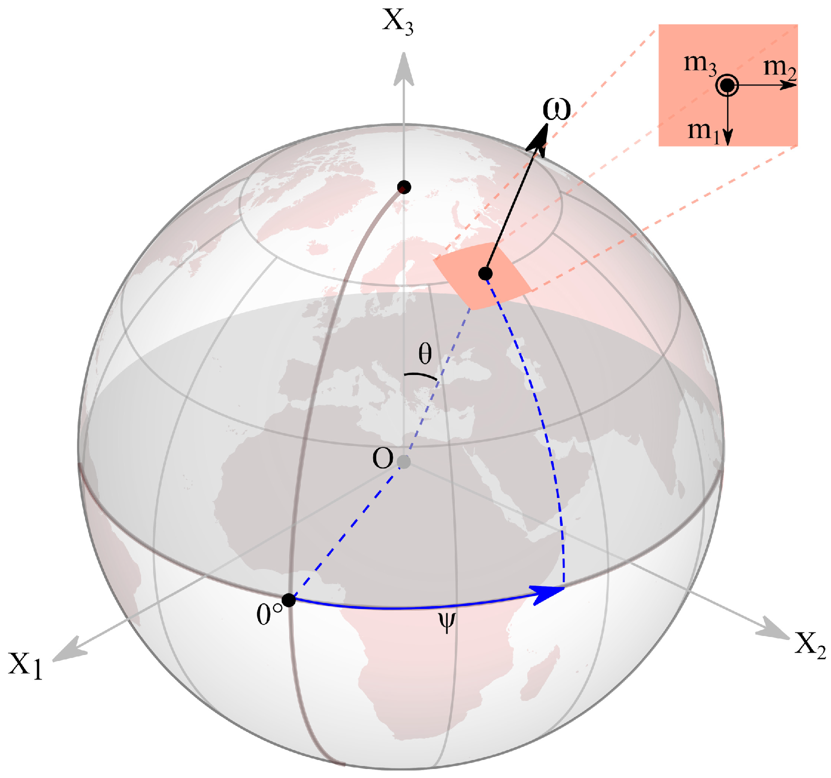
Lopes et al. [7] and Courtillot et al. [6] have recently recalled in some detail how Laplace [1] derived the system of differential equations that was later to be named Liouville-Euler. We call “full” polar motion the vector consisting of the two spherical coordinates of the pole and (according to the plane) and the third coordinate , linked to the length of the day (cf. Figure 1). The motion of the Earth’s rotation axis () can be seen as the combination of three Euler angles , and . The rotation axis moved only very small distances from its mean position (at least over the past century of continuous measurements) and one can write:
where Ω (= 7.292115 × 10⁻⁵ rad/s) is the Earth’s mean rotation velocity today computed on the last 3 decades. Applying the theorem of kinetic momentum to the rotation of a non-rigid body and following Lambeck [3], Chapter 3, Equations (1) lead to the set of Liouville-Euler equations (system 3.2.9 in Lambeck [3]):
where , , is the Euler frequency (), (=) and are the so-called excitation functions (e.g., [3], Chapter 4). C and A are respectively, the axial and equatorial moments of inertia of Earth (8.0365 × 1037 kg m2 and 8.010 × 1037 kg m2, [10]). In this derivation, the behavior of the pole position (m1, m2) and m3 have been fully separated. Through σr, (m1, m2) involve the (internal) terrestrial data C and A. Lambeck [3], page 34, writes: “m1 and m2 are the components of the polar motion or wobble and is nearly the acceleration in diurnal rotation”. The generally accepted reading (physical interpretation) of this formulation is that polar motion (m1, m2) is linked to geophysical excitation such as atmospheric or oceanic circulation, lithospheric and mantle convection or electromagnetic coupling, and that the m3 component is linked to astronomical phenomena such as tides. Lambeck [3], p. 36) concludes: “Equations (3.2.6) clearly separate the astronomical and geophysical problems”.
This is one reason for which on long time scales mechanical properties of the mantle are called upon. Some of these excitations can vary along with climate variations. Such is the case in the theory of isostasy (e.g., [11,12]). It is also the reason why one calls upon the ephemerids of the Moon and Sun in order to compute Earth tides (e.g., [13,14]) or to evaluate their influence on lod variations (e.g., [15,16]).
In the classical problem of the motion of a Lagrange top (e.g., [17]), the weight of the top plays the role of a perturbation of the full motion of the rotation axis. This is replaced by the astronomical torques of the Moon and Sun as excitations of the Earth’s rotation axis. This formalism has allowed one to compute the period of equinoctial precession (26,000 yr). This is how one is led to the Milankovitch theory of climate variations ([18]). The role of other bodies in the solar system, mainly the large and remote Jovian (gaseous) planets, must be taken into account (e.g., [19,20]), for they excite responses in eccentricity at very long periods (e.g., 400 kyr). As is the case for the top, changes in Earth rotation perturb its revolution about the Sun.
Laplace’s “classical” formulation of the theory is formally identical to the “modern” formulation recalled above ([3]). But it leads to a different sinterpretation reading. Laplace [1] deduces from the fundamental law of dynamics a system of equations that can be shown to be identical to (2). It reads ([1], page 74, system D):
On the left side of (3), (p, q, r) stand for the Euler angles (, and ) of Equation (1) and (p’, q’, r’) = (Cp, Aq, Br), still with (A, B, C) being the Earth’s moments of inertia. Let (x, y, z) be the coordinates of the Earth’s center of gravity, (x’, y’, z’) the coordinates of a mass element of Earth. Then:
are classical expressions for the second order inertia tensor. and are as defined is Figure 1. How can N, N’ and N” be evaluated without knowing the motions of all particles in and out of the Earth? In a bold move, Laplace [1], volume 1, book 5, page 305, paragraph 3, assumes that dN, dN’ and dN” can be computed from the positions and motions of the celestial bodies that act on it.
Laplace starts with the Sun, its mass L and distance r1. Equation (3) becomes:
This system is close to that proposed by Guinot [21], page 530, system 1:
Changing the directions of the axes and since B∼A, (5) and (6) are equivalent. But for Laplace, all terms on the right side are celestial (astronomical), whereas for Guinot the torques Lt, Mt and Nt (not to be mistaken for N in (3)) can be external or internal to the Earth. For the Laplace formulation, one must take into account all planets that can produce effects one wants to account for. For instance, Laplace gives the full equations with the Sun and Moon included:
The inclination of the rotation axis has the current value h in (7). is linked to the Earth’s rotation, therefore to the lod. On the right side of ((7) and (8)) are the ephemerids and masses of the Moon and Sun that enter the classical theory of gravitation (see Appendix A in Lopes et al. [7] for more details). Length of day and polar inclination are clearly connected by Equations (7) and (8). Thus, Laplace reduces the problem to a system of two equations for the inclination and time derivative of the declination of the Earth’s rotation axis. and (and the norm that can be considered as a known constant) give the direction of the polar rotation axis and its variations. The time difference (in ms) between the theoretical and measured Earth rotation is proportional to , v being the rotation velocity (and the Earth’s radius is a constant). Either alone, or v alone, or both can vary. We assume the former, since the mean rotation rate apparently remains constant, as was already noted above, and Equation (8) implies studying the time derivative of declination of the rotation axis, thus studying a quantity that is linearly related to the derivative of lod.
3. Confronting the Theory with the Observations
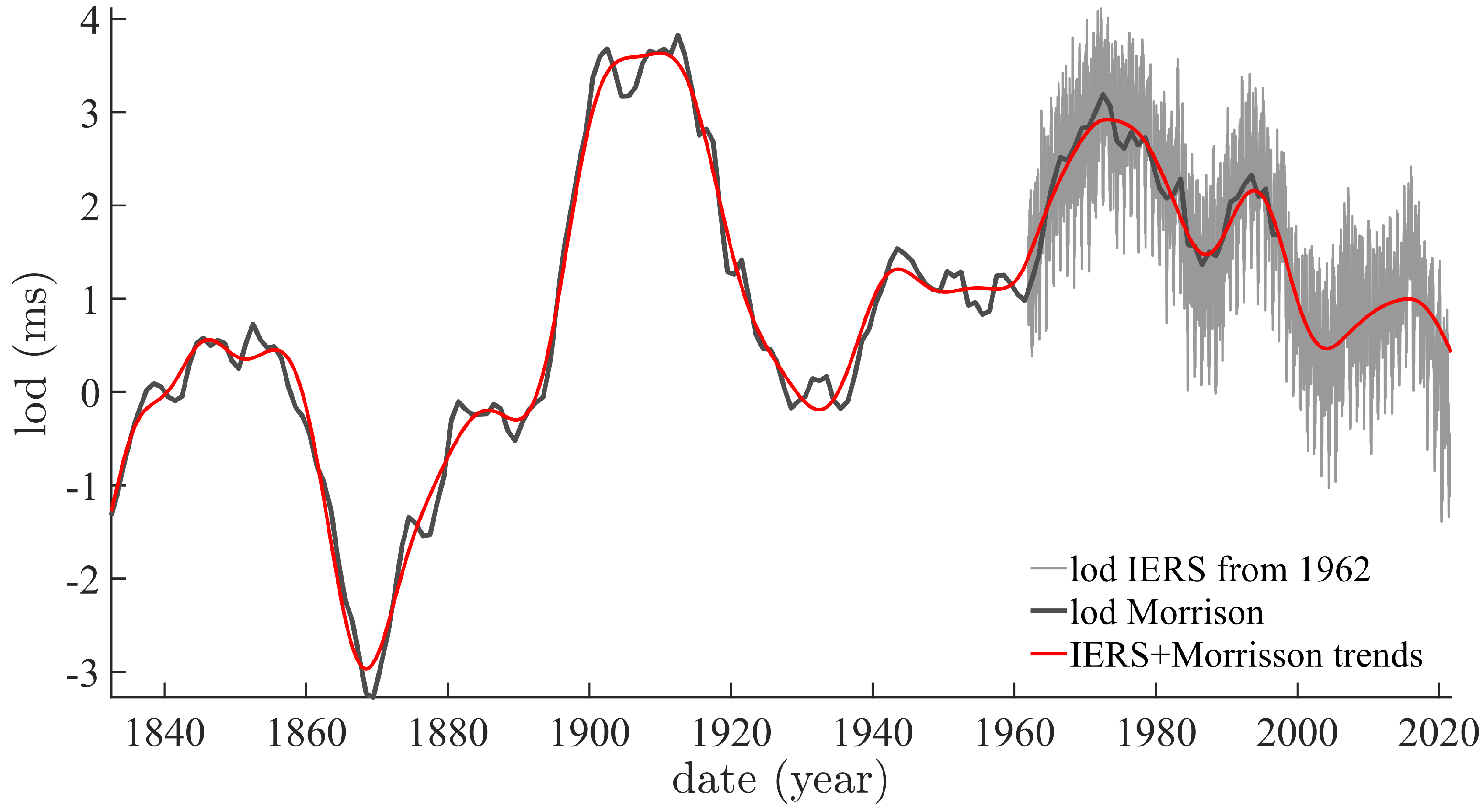
Stephenson and Morrison [22] have compiled the reference data for lod from 700AD onwards. This has allowed Gross [23] to build a monthly data set of lod from 1832 to 1997 (LUNAR97). We have combined it with the daily data provided by IERS (International Earth Rotation Service) since 1962 (https://www.iers.org/IERS/EN/DataProducts/data.html, accessed on 22 February 2022). Figure 2 shows the two data sets, and their (smoother) trends (the red curve). In order to determine these trends, we have applied iterative Singular Spectrum Analysis (iSSA; see [24,25,26,27]). The trends are the first, leading (in terms of pseudo-period and amplitude) components of the data series. The trends of the two series are smoothly continuous where they meet (1962).
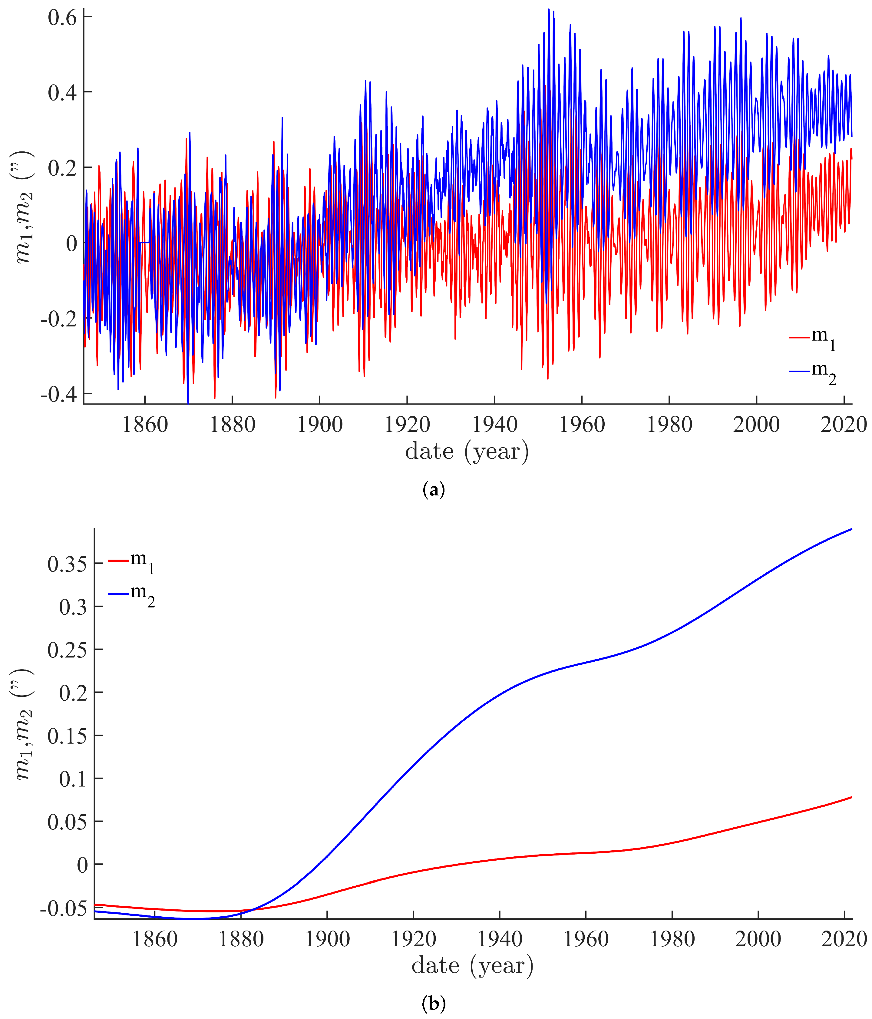
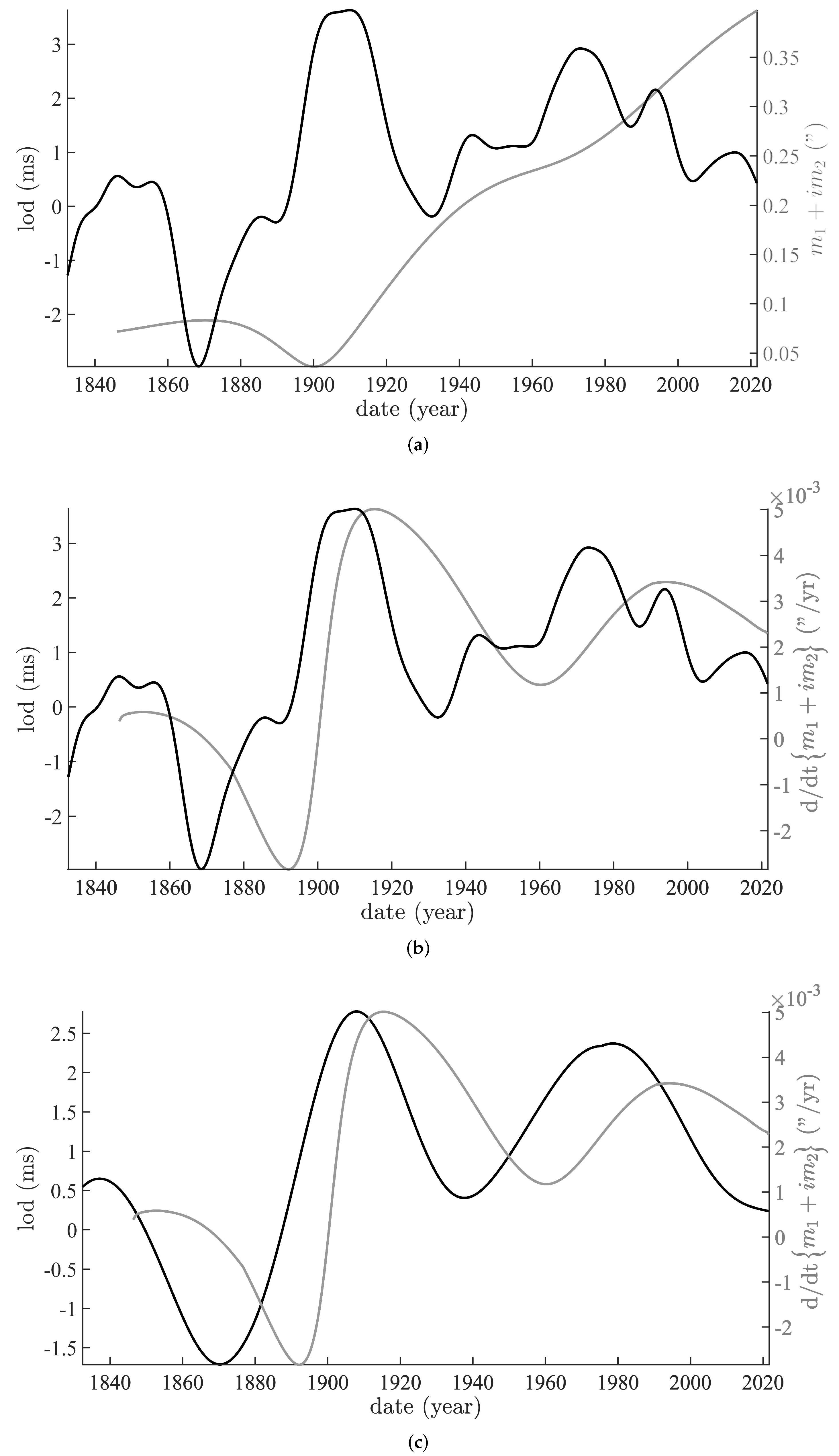
The data for the and components of polar motion since 1846 are also available from IERS and are shown in Figure 3a. Their respective trends, extracted by iSSA, are shown in Figure 3b. and are used to compute a global trend of m (), called the Markowitz drift ([28]). This is displayed in Figure 4a as a thinner gray curve, and compared to the Morrison/IERS trend of lod (thicker black curve). These curves are in excellent agreement with previous determinations (e.g., [29,30]), though they are smoother due to SSA extraction. We recall that the Markowitz drift is one of the three main components of polar motion along with the Chandler free oscillation and the forced annual oscillation (e.g., [7,31,32]). The magnitude of the Markowitz drift is on the same order as plate tectonic velocities, that originally made it quite difficult to detect.
Equations (7) and (8) imply an integrative link between θ and , that is polar motion and length of day. On Figure 4b, we show again the lod curve pictured in Figure 4a (thicker black curve) and the derivative of the Markowitz drift (thinner gray curve). Despite extraction by the textbfiSSA method, the lod curve is still affected by higher frequency variations. This may be due to the fact that the sampling rate jumps from monthly to daily in 1962 and to the presence of a derivative (that is a high-pass filter). We smooth further (moving average windows of 10 years) the lod curve (thicker black curve; Figure 4c) that is displayed with the derivative of the Markowitz drift already shown in Figure 4b (thinner gray curve).
The oscillatory smoothed trend of the Morisson/IERS lod peaks at ∼1905 and ∼1980, and the derivative of the Markowitz drift at ∼1915 and ∼2000, that is they have a similar period at ∼80 years. Equations (7) and (8) link the lod and the pole motion by a derivative operator; hence one should be in quadrature with respect to the other, that is 80/4 ∼20 years, as is observed (Figure 4c).
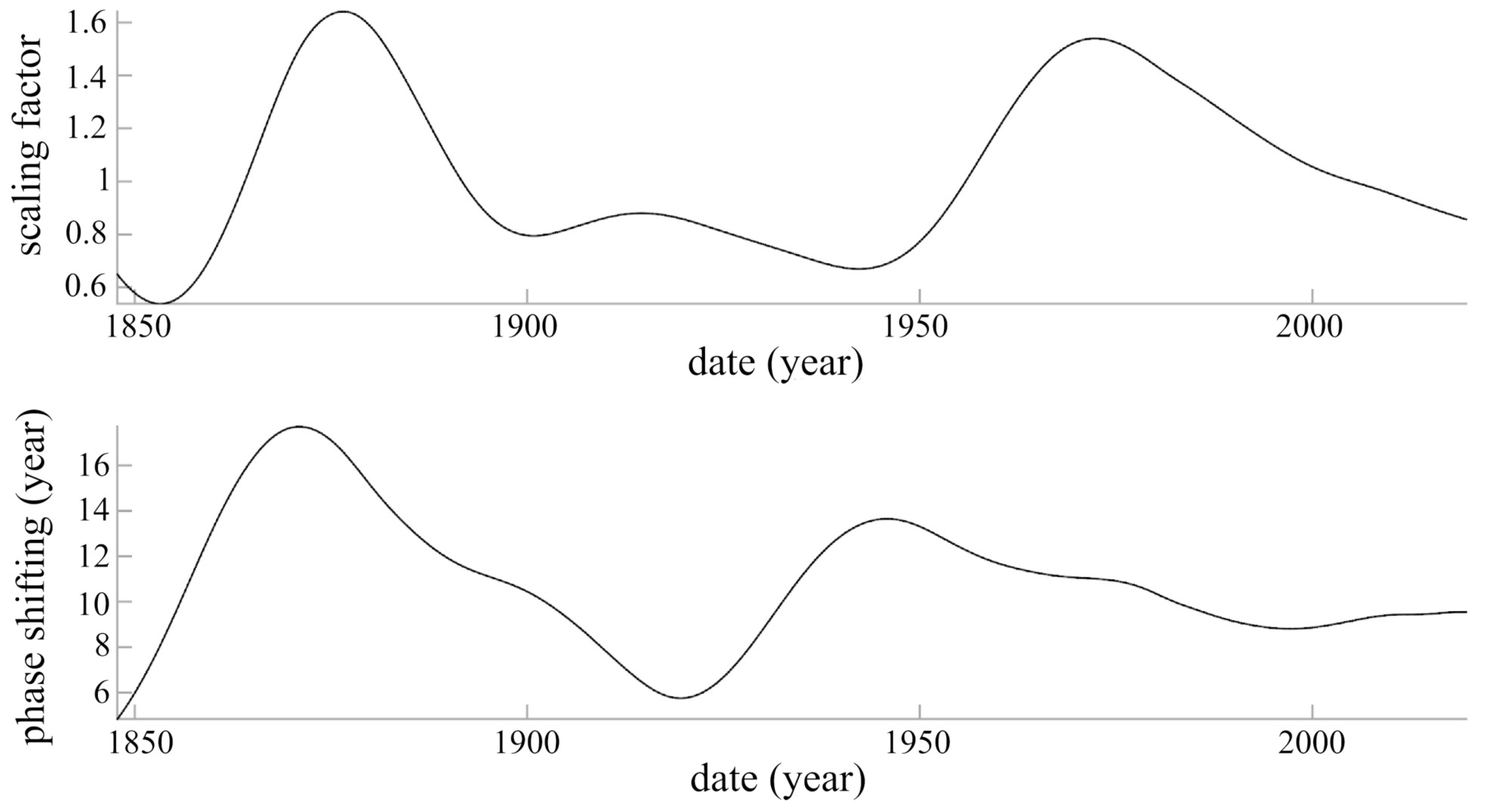
We have computed the relative phase and amplitude variations that would put the two curves in best agreement (normalized to take care of the different units). We have done this by applying the simulated annealing technique ([33]) in order to bring the pole motion curve of Figure 4c (gray curve) into superposition with lod (black curve).
Figure 5 shows the results, the amplitude and phase shift respectively at the top and bottom. We do not display the results of this inversion on waveforms since they are practically superposable (the dynamic time warping algorithm calculates the modulations of phase and amplitude of the operator that transforms the black curve of Figure 4c into the gray curve; the end result is two curves that are identical to 99%). The scaling factor (or amplitude of the operator) required to transform the normalized polar motion to the normalized lod ranges between 0.6 and 1.6 and averages 1.03 ± 0.30: to first order, the amplitudes of the two geophysical quantities m and lod evolve in parallel. The larger differences occur between 1870 and 1890, and a century later between 1970 and 1990 (Figure 5 top). The largest “jump” in both lod (4 ms) and pole motion (8 × 10⁻³″/yr) takes place between 1870 and 1900 (Figure 4c). The phase shift of that operator ranges between 6 and 16 years and averages 10.7 ± 3.0 yr. Note that during the period between 1920 and 1940, when the amplitude factor is close to a minimum (∼0.7), the Chandler free oscillation of polar motion suffers a well-known phase jump of .
4. Discussion and Concluding Remarks
Passing from the “classical” system of Equations (7) and (8), [1]) to the “modern” system of equations (2, e.g., [3]) is not complicated but is rather lengthy. There is no contradiction between the two formulations. However, each can be read with its own emphasis. The main difference between what Laplace and Poincaré write on one hand, and what Lambeck and Guinot write on the other hand arises at the step of system (3), leading either to (2) or to (Figure 4a,b). How does one account for system (4), that is for the distribution and motions of masses inside or outside Earth, at any place and instant? Laplace ssolves the point with resorts to a hypothesis: if one does not have access to masses and accelerations, one can still determine the force budget. For Laplace, these forces are exclusively external, leading to system (5), and then (7) and (8) with the Sun and Moon included. As a consequence, internal and external mass motions only serve to dissipate the energy received by polar motion from all celestial bodies (see Lopes et al. [7], Appendix 1). With Lambeck and Guinot’s formulation (2), one has to resort to purely terrestrial forces to explain mantle motions and changes in climate. Emphasis is on the separation between the polar coordinates (polar motion) and the third coordinate (linked to lod), and on determining the excitation functions, that can be external or internal to the Earth. These are mathematical functions that “include all factors that perturb the rotation motion” ([3], p. 36). These excitation functions are listed by [3], page 47: “the excitation functions consist of contributions from (i) redistribution of mass, (ii) relative motion of matter, and (iii) torques”, the difference between (i) and (ii) being tenuous. For Guinot (system (6)) the torques can be one or more external and internal actions.
In short, in the “modern” presentation, polar motion and length of day are decoupled and correspond to different physical mechanisms, whereas in the “classical” presentation polar motion involves coupling of the inclination of the rotation pole and the derivative of its declination.
In a previous SSA analysis of lod using more than 50 years of IERS observations, Le Mouël et al. [16] find nine components, all likely astronomical—thus external to the Earth (“trend”, ∼80 yr, 18.6 yr, 11 yr, 1 year, 0.5 yr, 27.54 days, 13.66 days, 13.63 days, 9.13 days). The QBO at 2.36 yr is interpreted as a Sun-related oscillation. The lunar components at 13.63 and 13.66 days could contain a solar contribution. The longer periods, 1 yr, 11 yr, 18.6 yr and ∼80 yr (Markowitz, Figure 4c) are common to lod and polar motion. If the link between the two is as established by Laplace [1], then the straightening of the inclination of the axis of rotation swould should accompany a decrease in lod, and indeed the Earth currently s.The Earth indeed straightens up (cf. Stoyko [29] and Figure 3b). Also, if this link is valid, all the components with extraterrestrial periods should be present in the series of sunspots; and indeed they are (e.g., Courtillot et al. [6]). As far as quasi annual components of sunspots are concerned, there is no exact 1 yr line, but two nearby lines with periods 0.93 and 1.05 yr (Le Mouël et al. [34], Table 1),that could be luni-solar commensurabilities (365.25-28)/365.25 = 0.92 and (365.25 + 28)/365.25 = 1.07, 28 days being the Moon’s synodic period (cf. Courtillot et al. [6]; Lopes et al. [7]; Bank and Scafetta [35]). Can a sufficiently strong source of energy be found? Indeed it has been known for some time (e.g., Dickman [36]; Chao et al. [37]; Varga et al. [38]) and confirmed recently by Le Mouël [16] that the components with luni-solar periods found above account for 95% of the total variance of the lod signal.
Another benefit of using the original Laplace approach is the straightforward determination of the period of the Euler free oscillation. In one of the first analyses of actual observations of polar motion, Chandler [39,40] discovered the wobble that now bears his name. Chandler wrote that “textitthe general result of a preliminary discussion is to show a revolution of the earth’s pole in a period of 427 days.” The observed period of this free oscillation is much larger than the theoretical value of 306 days, even more so now that the period has reached about 433 days (e.g., [32,41]). As noted at the end of Section 3, the envelope of the Chandler oscillation is strongly modulated, reaching a quasi-minimum around 1930 with its well known phase jump of . The duration and the modulation of the Chandler wobble require a source of excitation. Earth elasticity, large earthquakes (e.g., [42,43,44,45]), or external forcing by the fluid envelopes (e.g., [3] Chapter 7, [46,47,48,49,50]) have been successively invoked in the “modern” viewpoint.
In the “classical” reading of Laplace, still considering an elastic (or plastic) Earth, we have seen that the Equations (7) and (8) allow one to calculate the period of the Euler free oscillation. This oscillation actually varies with the pole inclination from 306 to 578 days. A transition to a double period (∼430 and ∼433 days) has taken place at the time of the 1930 phase jump of the Chandler oscillation; this can be accounted for by variations in polar inclination (cf. Figure 4c). As is the case for a top, as recalled in Section 2, the various rotations (precession, etc.…) vary with the inclination of the rotation axis.
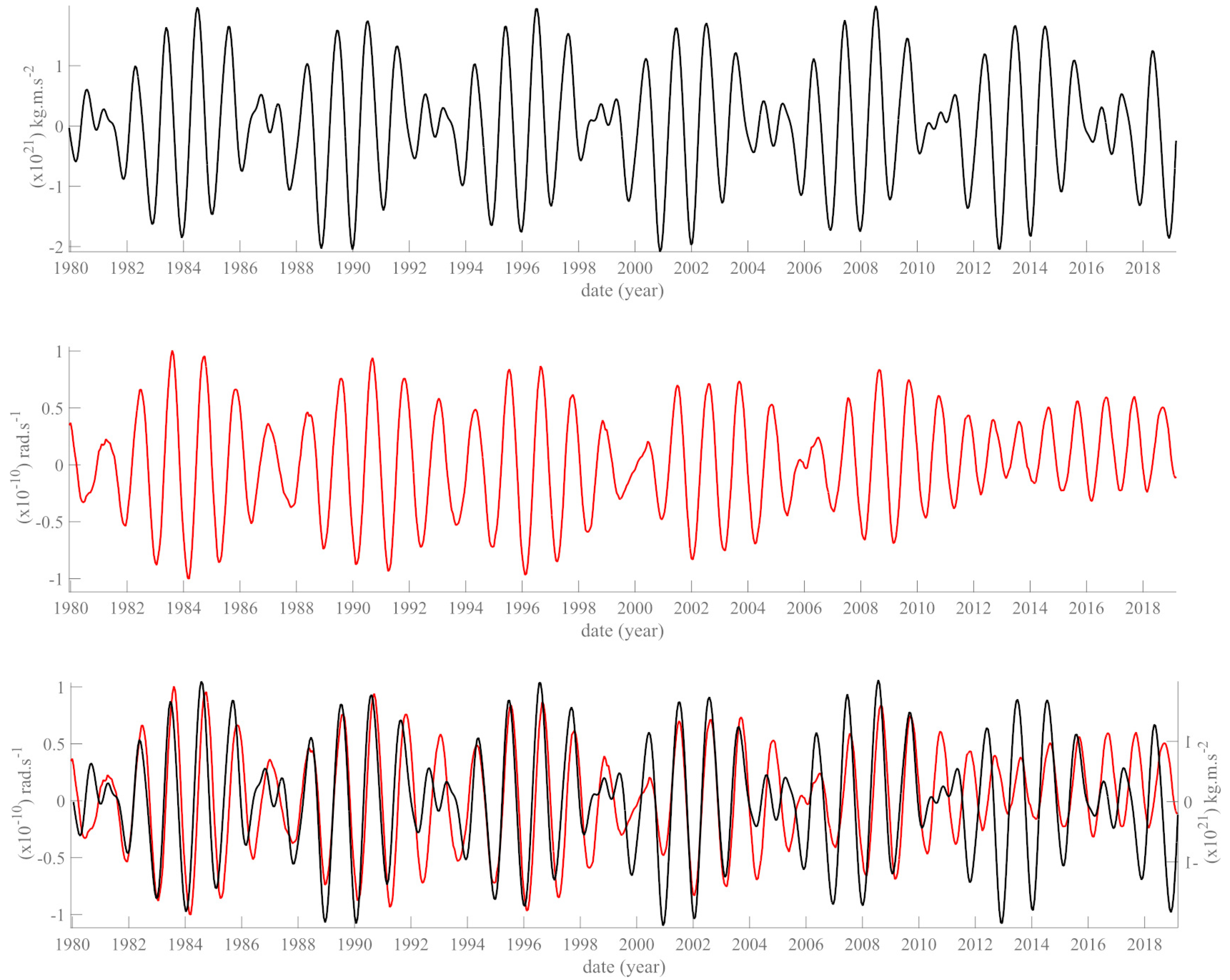
Laplace [1] calculations and conclusions have been confirmed, prominently by Poincaré [2]. Based on these equations, a link between the rotations and the torques exerted by the planets of our solar system is expected. Indeed, we have shown elsewhere the influence of Jovian planets on the Sun (sunspots, cf. [6]), and Earth ([7], Figure 11). In the latter paper, we show the similarity between the envelope of the Chandler oscillation and the ephemerids of Neptune. Figure 3 of Lopes et al. [7], reproduced here as Figure 6, shows the remarkable agreement between the sum of forces exerted by the four Jovian planets and the component of polar motion.
As far as the length of day is concerned, we have seen in Figure 2 that since 1970 it tends to decrease, i.e., the Earth’s velocity of rotation tends to increase. The same phenomena envisioned above (earthquakes, variations in the fluid envelopes, …) have been proposed as potential causes of this trend (e.g., [46,51,52,53,54]). But the recent acceleration of rotation velocity, that contradicts previous models, may find a simple explanation with Laplace’s formalism (e.g., [55]).
Although several of the points made in this paper have been known to physicists, they may not have been to many geoscientists. We believe there is value in following Laplace’s approach: it leads to the suggestion that all the oscillatory components with extraterrestrial periods should be present in the series of sunspots and indeed they are. In closing, we emphasize that all he quantitative results obtained in his paper are based on actual data and the validity of Laplace’s astronomical hypothesis, not on a model.
Author Contributions
V.C., J.-L.L.M., F.L. and D.G. contributed to conceptualization, formal analysis, interpretation and writing. All authors have read and agreed to the published version of the manuscript.
Funding
This research was supported by the Université de Paris, IPGP and the LGL-TPE de Lyon.
Data Availability Statement
The used data are freely available at the following address: Met Office Hadley Centre: https://www.metoffice.gov.uk/hadobs/hadslp2/data/download.html (accessed on 10 October 2020) IERS: https://www.iers.org/IERS/EN/DataProducts/EarthOrientationData/eop.html (accessed on 12 October 2020).
Acknowledgments
We thank the anonymous reviewers for their helpful comments on the manuscript.
Conflicts of Interest
The authors declare that they have no known competing financial interests or personal relationships that could have appeared to influence the work reported in this paper.
References
- Laplace, P.S. Traité de Mécanique Céleste; l’Imprimerie de Crapelet: Paris, France, 1799. [Google Scholar]
- Poincaré, H. Les Méthodes Nouvelles de la Mécanique Céleste; Gauthier-Villars: Paris, France, 1893. [Google Scholar]
- Lambeck, K. The Earth’s Variable Rotation: Geophysical Causes and Consequences; Cambridge University Press: Cambridge, UK, 2005. [Google Scholar]
- Abreu, J.A.; Beer, J.; Ferriz-Mas, A.; McCracken, K.G.; Steinhilber, F. Is there a planetary influence on solar activity? Astron. Astrophys. 2012, 548, A88. [Google Scholar] [CrossRef] [Green Version]
- Scafetta, N. Solar oscillations and the orbital invariant inequalities of the solar system. Sol. Phys. 2020, 295, 33. [Google Scholar] [CrossRef]
- Courtillot, V.; Lopes, F.; Le Mouël, J.L. On the prediction of solar cycles. Sol. Phys. 2021, 296, 21. [Google Scholar] [CrossRef]
- Lopes, F.; Le Mouël, J.L.; Courtillot, V.; Gibert, D. On the shoulders of Laplace. Phys. Earth Planet. Inter. 2021, 316, 106693. [Google Scholar] [CrossRef]
- Le Mouël, J.L.; Lopes, F.; Courtillot, V. Identification of Gleissberg cycles and a rising trend in a 315-year-long series of sunspot numbers. Sol. Phys. 2017, 292, 43. [Google Scholar] [CrossRef]
- Le Mouël, J.L.; Lopes, F.; Courtillot, V. Sea-Level Change at the Brest (France) Tide Gauge and the Markowitz Component of Earth’s Rotation. J. Coast. Res. 2021, 37, 683–690. [Google Scholar] [CrossRef]
- Chen, W.; Shen, W. New estimates of the inertia tensor and rotation of the triaxial nonrigid Earth. J. Geophys. Res. Solid Earth 2010, 115, B12. [Google Scholar] [CrossRef]
- Peltier, W.R.; Andrews, J.T. Glacial-isostatic adjustment—I. The forward problem. Geophys. J. Int. 1976, 46, 605–646. [Google Scholar] [CrossRef]
- Nakiboglu, S.M.; Lambeck, K. Deglaciation effects on the rotation of the Earth. Geophys. J. Int. 1980, 62, 49–58. [Google Scholar] [CrossRef] [Green Version]
- Melchior, P. The Earth Tides; Pergamon Press: Oxford, UK, 1966; 458p. [Google Scholar]
- Ray, R.D.; Erofeeva, S.Y. Long-period tidal variations in the length of day. J. Geophys. Res. Solid Earth 2014, 119, 1498–1509. [Google Scholar] [CrossRef]
- Wahr, J.M.; Sasao, T.; Smith, M.L. Effect of the fluid core on changes in the length of day due to long period tides. Geophys. J. Int. 1981, 64, 635–650. [Google Scholar] [CrossRef]
- Le Mouël, J.L.; Lopes, F.; Courtillot, V.; Gibert, D. On forcings of length of day changes: From 9-day to 18.6-year oscillations. Phys. Earth Planet. Inter. 2019, 292, 1–11. [Google Scholar] [CrossRef]
- Lagrange, J.L. Mécanique Analytique; Mallet-Bachelier: Paris, France, 1853. [Google Scholar]
- Milanković, M. Théorie Mathématique des Phénomènes Thermiques Produits par la Radiation Solaire; Gauthier-Villars: Paris, France, 1920. [Google Scholar]
- Laskar, J.; Robutel, P.; Joutel, F.; Gastineau, M.; Correia, A.C.M.; Levrard, B. A long-term numerical solution for the insolation quantities of the Earth. Astron. Astrophys. 2004, 428, 261–285. [Google Scholar] [CrossRef] [Green Version]
- Laskar, J.; Fienga, A.; Gastineau, M.; Manche, H. La2010: A new orbital solution for the long-term motion of the Earth. Astron. Astrophys. 2011, 532, A89. [Google Scholar] [CrossRef]
- Guinot, B. Variation du pôle et de la vitesse de rotation de la Terre, ch. 19. In Traité de Géophysique Interne; Coulomb, J., Jobert, G., Eds.; Masson: Paris, France, 1976; Volume 1, pp. 529–564. [Google Scholar]
- Stephenson, F.R.; Morrison, L.V. Long-term changes in the rotation of the Earth: 700 BC to AD 1980. Philos. Trans. Royal Soc. A 1984, 313, 47–70. [Google Scholar] [CrossRef]
- Gross, R.S. A combined length-of-day series spanning 1832–1997: LUNAR97. Phys. Earth Planet. Inter. 2001, 123, 65–76. [Google Scholar] [CrossRef]
- Golyandina, N.; Zhigljavsky, A. Singular Spectrum Analysis for Time Series; Springer: Berlin/Heidelberg, Germany, 2013; Volume 120, ISBN 978-3642349126. [Google Scholar]
- Lemmerling, P.; Van Huffel, S. Analysis of the structured total least squares problem for hankel/toeplitz matrices. Numer. Algorithms 2001, 27, 89–114. [Google Scholar] [CrossRef]
- Golub, G.H.; Reinsch, C. Singular value decomposition and least squares solutions. In Linear Algebra; Springer: Berlin/Heidelberg, Germany, 1971; pp. 134–151. [Google Scholar]
- Lopes, F.; Courtillot, V.; Le Mouël, J.-L. Triskeles and Symmetries of Mean Global Sea-Level Pressure. Atmosphere 2022, 13, 1354. [Google Scholar] [CrossRef]
- Markowitz, W. Concurrent astronomical observations for studying continental drift, polar motion, and the rotation of the Earth. In Symposium-International Astronomical Union; Cambridge University Press: Cambridge, UK, 1968; Volume 32, pp. 25–32. [Google Scholar]
- Stoyko, A. Mouvement seculaire du pole et la variation des latitudes des stations du SIL. In Symposium-International Astronomical Union; Cambridge University Press: Cambridge, UK, 1968; Volume 32, pp. 52–56. [Google Scholar]
- Hulot, G.; Le Huy, M.; Le Mouël, J.L. Influence of core flows on the decade variations of the polar motion. Geophys. Astrophys. Fluid Dyn. 1996, 82, 35–67. [Google Scholar] [CrossRef]
- Gibert, D.; Holschneider, M.; Le Mouël, J.L. Wavelet analysis of the Chandler wobble. J. Geophys. Res. Solid Earth 1998, 103, 27069–27089. [Google Scholar] [CrossRef]
- Zotov, L.; Bizouard, C. On modulations of the Chandler wobble excitation. J. Geodyn. 2012, 62, 30–34. [Google Scholar] [CrossRef]
- Kirkpatrick, S.; Gelatt, C.D., Jr.; Vecchi, M.P. Optimization by simulated annealing. Science 1983, 220, 671–680. [Google Scholar] [CrossRef]
- Le Mouël, J.L.; Lopes, F.; Courtillot, V. Solar turbulence from sunspot records. Mon. Not. R. Astron. Soc. 2020, 492, 1416–1420. [Google Scholar] [CrossRef]
- Bank, M.J.; Scafetta, N. Scaling, mirror symmetries and musical consonances among the distances of the planets of the solar system. arXiv 2022, arXiv:2202.03939. [Google Scholar] [CrossRef]
- Dickman, S.R. A complete spherical harmonic approach to luni-solar tides. Geophys. J. Int. 1989, 99, 457–468. [Google Scholar] [CrossRef] [Green Version]
- Chao, B.F.; Merriam, J.B.; Tamura, Y. Geophysical analysis of zonal tidal signals in length of day. Geophys. J. Int. 1995, 122, 765–775. [Google Scholar] [CrossRef] [Green Version]
- Varga, P.; Gambis, D.; Bizouard, C.; Bus, Z.; Kiszely, M. Tidal influence through LOD variations on the temporal distribution of earthquake occurrences. In Proceedings of the Journées 2005 “Systèmes de Référence Spatio-temporels”: Earth Dynamics and Reference Systems: Five Years after the Adoption of the IAU 2000 Resolutions, Held at Space Research Centre PAS, Warsaw, Poland, 19–21 September 2005. [Google Scholar]
- Chandler, S.C. On the variation of latitude, I. Astron. J. 1891, 11, 59–61. [Google Scholar] [CrossRef]
- Chandler, S.C. On the variation of latitude, II. Astron. J. 1891, 11, 65–70. [Google Scholar] [CrossRef]
- Lopes, F.; Le Mouël, J.L.; Gibert, D. The mantle rotation pole position. A solar component. Comptes Rendus Geosci. 2017, 349, 159–164. [Google Scholar] [CrossRef]
- Mansinha, L.; Smylie, D.E. Effect of earthquakes on the Chandler wobble and the secular polar shift. J. Geophys. Res. Atmos. 1967, 72, 4731–4743. [Google Scholar] [CrossRef]
- Dahlen, F.A. The excitation of the Chandler wobble by earthquakes. Geophys. J. Int. 1971, 25, 157–206. [Google Scholar] [CrossRef] [Green Version]
- O’Connell, R.J.; Dziewonski, A.M. Excitation of the Chandler wobble by large earthquakes. Nature 1976, 262, 259–262. [Google Scholar] [CrossRef]
- Gross, R.S. The influence of earthquakes on the Chandler wobble during 1977–1983. Geophys. J. Int. 1986, 85, 161–177. [Google Scholar] [CrossRef] [Green Version]
- Rochester, M.G. Causes of fluctuations in the rotation of the Earth. Philos. Trans. R. Soc. A 1984, 313, 95–105. [Google Scholar] [CrossRef]
- Gross, R.S. The excitation of the Chandler wobble. Geophys. Res. Lett. 2000, 27, 2329–2332. [Google Scholar] [CrossRef] [Green Version]
- Aoyama, Y.; Naito, I. Atmospheric excitation of the Chandler wobble, 1983–1998. J. Geophys. Res. Solid Earth 2001, 106, 8941–8954. [Google Scholar] [CrossRef]
- Brzeziński, A.; Nastula, J. Oceanic excitation of the Chandler wobble. Adv. Space Res. 2002, 30, 195–200. [Google Scholar] [CrossRef]
- Desai, S.D. Observing the pole tide with satellite altimetry. J. Geophys. Res. Oceans 2002, 107, 7-1–7-13. [Google Scholar] [CrossRef]
- Gross, R.S.; Fukumori, I.; Menemenlis, D.; Gegout, P. Atmospheric and oceanic excitation of length-of-day variations during 1980–2000. J. Geophys. Res. Solid Earth 2004, 109, B1. [Google Scholar] [CrossRef]
- Landerer, F.W.; Jungclaus, J.H.; Marotzke, J. Ocean bottom pressure changes lead to a decreasing length-of-day in a warming climate. Geophys. Res. Lett. 2007, 34. [Google Scholar] [CrossRef]
- Chen, J.; Wilson, C.R.; Kuang, W.; Chao, B.F. Interannual oscillations in earth rotation. J. Geophys. Res. Solid Earth 2019, 124, 13404–13414. [Google Scholar] [CrossRef]
- Afroosa, M.; Rohith, B.; Paul, A.; Durand, F.; Bourdallé-Badie, R.; Sreedevi, P.V.; Shenoi, S.S.C. Madden-Julian oscillation winds excite an intraseasonal see-saw of ocean mass that affects Earth’s polar motion. Commun. Earth Environ. 2001, 2, 139. [Google Scholar] [CrossRef]
- Trofimov, D.A.; Petrov, S.D.; Movsesyan, P.V.; Zheltova, K.V.; Kiyaev, V.I. Recent acceleration of the Earth rotation in the summer of 2020: Possible causes and effects. J. Phys. Conf. Ser. 2021, 2103, 012039. [Google Scholar] [CrossRef]
Figure 1.
Terrestrial reference frame. and are the coordinates of the rotation pole. and are the declination and inclination introduced by Laplace [1].
Figure 1.
Terrestrial reference frame. and are the coordinates of the rotation pole. and are the declination and inclination introduced by Laplace [1].

Figure 2.
Monthly values of length of day data (LUNAR97, 1832–1997; bold black curve) from Gross [23] and daily values (1962–Present, gray curve) from IERS. Superimposed are their trends as determined by SSA (LUNAR97 + IERS = red curve).
Figure 2.
Monthly values of length of day data (LUNAR97, 1832–1997; bold black curve) from Gross [23] and daily values (1962–Present, gray curve) from IERS. Superimposed are their trends as determined by SSA (LUNAR97 + IERS = red curve).

Figure 3.
Polar motion from IERS. (a) The and components of polar motion from IERS (from 1846 to the Present). (b) The trends of components and from 1846 to the Present, extracted using SSA.
Figure 3.
Polar motion from IERS. (a) The and components of polar motion from IERS (from 1846 to the Present). (b) The trends of components and from 1846 to the Present, extracted using SSA.

Figure 4.
Polar motion from IERS (a) Comparison of the trends of the Morisson/IERS lod (black) and of polar motion m (gray). (b) Comparison of the trend of the Morisson/IERS lod (black) and of the derivative of the Markowitz drift (gray). (c) Comparison of the smoothed trend of the Morisson/IERS lod (black) and of the derivative of the Markowitz drift (gray).

Figure 5.
Scaling factor (top) and phase shift (bottom) of the operator that brings the two curves of Figure 4c in best agreement from 1846 to the Present.
Figure 5.
Scaling factor (top) and phase shift (bottom) of the operator that brings the two curves of Figure 4c in best agreement from 1846 to the Present.

Figure 6.
Top curve (in black): the sum of the forces of the four Jovian planets affecting Earth (ephemerids from the IMCCE). Middle curve (in red): the component of polar motion (1980–2019), reconstructed with SSA and with the trend (Markowitz) removed. Bottom: superposition of the 2 curves. From Lopes et al. [7], Figure 3.

Publisher’s Note: MDPI stays neutral with regard to jurisdictional claims in published maps and institutional affiliations. |
© 2022 by the authors. Licensee MDPI, Basel, Switzerland. This article is an open access article distributed under the terms and conditions of the Creative Commons Attribution (CC BY) license (https://creativecommons.org/licenses/by/4.0/).
Share and Cite
MDPI and ACS Style
Lopes, F.; Courtillot, V.; Gibert, D.; Mouël, J.-L.L. On Two Formulations of Polar Motion and Identification of Its Sources. Geosciences 2022, 12, 398. https://0-doi-org.brum.beds.ac.uk/10.3390/geosciences12110398
AMA Style
Lopes F, Courtillot V, Gibert D, Mouël J-LL. On Two Formulations of Polar Motion and Identification of Its Sources. Geosciences. 2022; 12(11):398. https://0-doi-org.brum.beds.ac.uk/10.3390/geosciences12110398
Chicago/Turabian StyleLopes, Fernando, Vincent Courtillot, Dominique Gibert, and Jean-Louis Le Mouël. 2022. "On Two Formulations of Polar Motion and Identification of Its Sources" Geosciences 12, no. 11: 398. https://0-doi-org.brum.beds.ac.uk/10.3390/geosciences12110398
Note that from the first issue of 2016, this journal uses article numbers instead of page numbers. See further details here.