Revisiting of a Three-Parameter One-Dimensional Vertical Infiltration Equation

Abstract

In the present study, the three-parameter one-dimensional vertical infiltration equation recently proposed by Poulovassilis and Argyrokastritis is examined. The equation includes the saturated hydraulic conductivity (K_s), soil sorptivity (S), and an additional parameter c; it is valid for all infiltration times. The c parameter is a fitting parameter that depends on the type of porous medium. The equation is characterized by the incorporation of the exact contribution of the pressure head gradient to flow during the vertical infiltration process. The application of the equation in eight porous media showed that it approaches to the known two-parameter Green–Ampt infiltration equation for parameter c = 0.300, while it approaches to the two-parameter infiltration equation of Talsma–Parlange for c = 0.750, which are the two extreme limits of the cumulative infiltration of soils. The c parameter value of 0.500 can be representative of the infiltration behavior of many soils for non-ponded conditions, and consequently, the equation can be converted into a two-parameter one. The determination of K_s, S, and c using one-dimensional vertical infiltration data from eight soils was also investigated with the help of the Excel Solver application. The results showed that when all three parameters are considered as adjustment parameters, accurate predictions of S and K_s are not achieved, while if the parameter c is fixed at 0.500, the prediction of S and K_s is very satisfactory. Specifically, in the first case, the maximum relative error values were 33.29% and 39.53% for S and K_s, respectively, while for the second case, the corresponding values were 13.25% and 17.42%.

1. Introduction

The phenomenon of infiltration plays a key role in hydrology, irrigation, and environmental studies. Several models have been proposed to describe the relationship between vertical cumulative infiltration in homogeneous soil and infiltration time i(t). These models can be classified into three categories [1,2], the physical models [3,4,5,6], semi-empirical models [7,8,9], and empirical models [9,10].

In many cases, comparative results from different models describing vertical infiltration have been presented [11,12,13,14,15]. However, between the compared models, there is a difference in the number of physical or fitting parameters. Most of the afore mentioned models are two-parameter models with the parameters of soil sorptivity, S (characterizing the ability of soil to drive water by capillarity) and saturated hydraulic conductivity, K_s (characterizing the ability of soil to conduct water by gravity) [16].

Poulovassilis and Argyrokastritis [17] presented a two term three-parameter infiltration model (Equation (1)) which includes, in addition to K_s and S, the parameter c, and is valid for all infiltration times. The c is a fitting parameter and depends on the type of the porous medium.

$$\mathrm{i}=\mathrm{S}\sqrt{\mathrm{t}}{\mathrm{e}}^{\left(-\mathrm{c}\left(\frac{{\mathrm{K}}_{\mathrm{s}}}{\mathrm{S}}\right)\sqrt{\mathrm{t}}\right)}+{\mathrm{K}}_{\mathrm{s}}\mathrm{t}$$

(1)

In addition, this equation has the advantage of the explicit form of i as function of t.

The equation incorporates the exact contribution of the pressure head gradient term to flow during the vertical infiltration process in a homogenous soil for non-ponded conditions and satisfies the physics of the infiltration phenomenon. It is documented that this contribution is smaller than the corresponding one of the pressure head gradient during horizontal infiltration by a time-dependent factor characteristic of each porous medium. Poulovassilis and Argyrokastritis [17] reported that deviations observed between various infiltration models and experimental data were generally attributed to non-incorporating the exact contribution of the pressure head gradient term to the flow in the infiltration model. They also suggested the fixed value of c = 0.6 for acceptable values of cumulative infiltration (i), and consequently, the model is converted to a two-parameter infiltration model.

Three-parameter infiltration equations have been proposed by Brutsaert [18], Swartzendruber [6], and Parlange et al. [19]. Usually, for practical purposes, for the third parameter they suggested a fixed value, and thus their equations are converted to two-parameter ones. Specifically, Brutsaert [18] proposed the constant value 1, Swartzendruber [6] the value 0.75, and Parlange et al. [19] the value 0.85.

Parlange et al. [19] found that when the third parameter tends to 0, their equation is converted into the Green–Ampt equation (Equation (2)) [3], while when it tends to 1, it is converted into the Talsma–Parlange equation (Equation (3)) [20], which are the two extreme limiting infiltration equations. Both equations are characterized by implicitness in i but explicitness in t.

$$\mathrm{t}=\frac{\mathrm{i}}{{\mathrm{K}}_{\mathrm{s}}}-\frac{{\mathrm{S}}^2}{2{\mathrm{K}}_{\mathrm{s}}^2}\ln \left(1+\frac{2{\mathrm{K}}_{\mathrm{s}}\mathrm{i}}{{\mathrm{S}}^2}\right)$$

(2)

$$\mathrm{t}=\frac{\mathrm{i}}{{\mathrm{K}}_{\mathrm{s}}}+\frac{{\mathrm{S}}^2}{2{\mathrm{K}}_{\mathrm{s}}^2}\left(\exp \left(-\frac{2{\mathrm{K}}_{\mathrm{s}}\mathrm{i}}{{\mathrm{S}}^2}\right)-1\right)$$

(3)

The issue of a corresponding investigation of the range of parameter c values in the Poulovassilis and Argyrokastritis [17] equation and whether a fixed value of c can lead to reliable values of i(t) remains open.

In addition, cumulative infiltration data can be used to estimate soil hydraulic properties with proper analysis. Commonly, the S and K_s parameters are searched out, which are characterized by Vrugt and Gao [21] as super-parameters of the hydraulic functions. Generally, two methods have been proposed to estimate K_s and S from cumulative infiltration models [22]: the linearization methods [23,24,25] and the curve fitting methods based on an inverting procedure to estimate S and K_s [26,27,28,29,30].

While relatively extensive research has been done on the reliability of S and K_s predictions from two- or three-parameter infiltration equations, using mainly the inverting procedure, no corresponding research on the Poulovassilis and Argyrokastritis [17] equation has been done so far. Clothier and Scotter [31], Rahmati et al. [14], and Kargas et al. [16] have reported that one can use the Data Solver application in Excel to minimize the objective function between the experimental infiltration data and the predicted ones to predict the parameters S and K_s. In general, in the case of three-parameter infiltration equations, when the third parameter is also considered as adjustment parameter, the predictions of S and K_s are not improved. For this reason, it is usually recommended to use a fixed value of the third parameter [14,16,30,32]. In addition, a key issue is the role of infiltration time in reliable prediction of S and K_s. Latorre et al. [32] showed that even short infiltration times are sufficient for accurate prediction of S, while much longer times (i.e., 1000 s) are required for the prediction of K_s in the case of the equation of Parlange et al. [19]. However, a systematic investigation of the above mentioned in the case of the equation of Poulovassilis and Argyrokastritis [17] has not been carried out until now.

The objectives of this study are: (1) To investigate the range of the value of the parameter c and to find, if possible, a fixed value for a reliable estimation of cumulative infiltration. (2) To check the accuracy of the hydraulic properties (S and K_s) estimation by applying the non-linear optimization method using the Excel Solver tool (a) for the simultaneous calculation of the values of the three parameters and (b) considering the parameter c as fixed. (3) To investigate the role of infiltration time in the estimation of S and K_s.

2. Materials and Methods

2.1. Porous Media

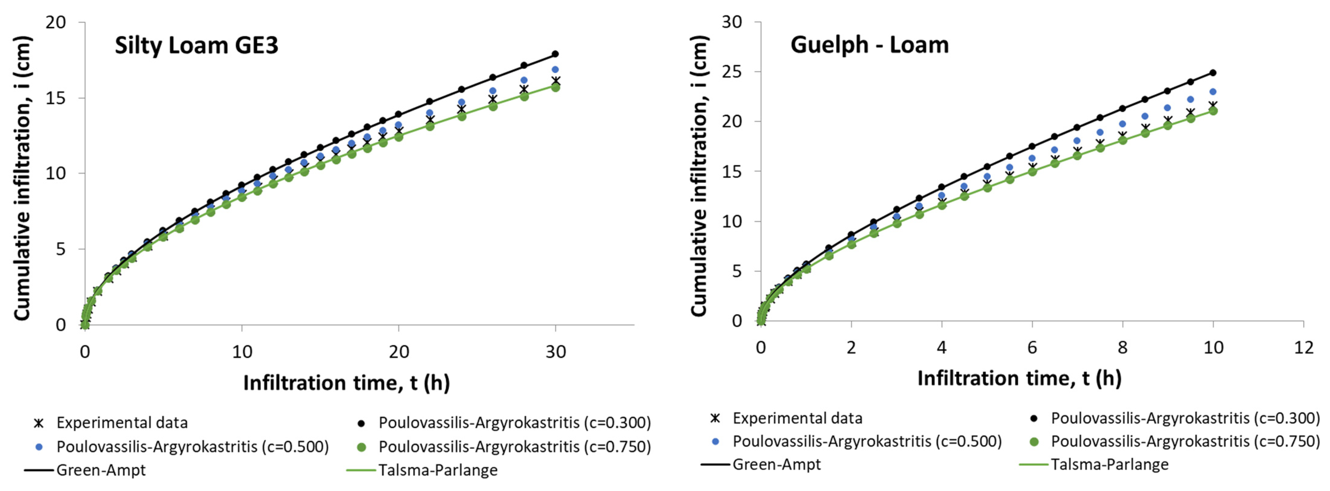
Experimentally or numerically one-dimensional vertical infiltration data obtained by applying a surface ponding depth (H ≥ 0), from eight different porous media, were studied. Specifically, the experimental infiltration data were obtained: (a) from the literature and concern the porous media: Sandy Soil-Grenoble with H = 2.25 cm [12] and Silty soil with H = 0 cm [13]; (b) from experiments conducted on a Sandy Loam soil with H = 3 cm [16]. The numerical infiltration data concern the porous media: Yolo Light Clay with H = 0 cm [13], Sand with H = 0 cm [13], and Soil and Sand mixture with H = 0 cm [13].

The remaining two porous media are the Silty Loam GE3 [33] and the Guelph Loam [33], for which their soil water retention and hydraulic conductivity curves are described from the van Genuchteen [33]-Mualem [34] model [25]. Vertical infiltration was numerically simulated by using the HYDRUS-1D Code [27], with an initial pressure head of −500 cm and surface ponding depth of 0 cm for both porous media. At the lower boundary of the 1 m uniform soil profile, a zero-pressure head gradient was defined (free drainage).

The values of K_s and S for the Sandy Soil-Grenoble soil are reported by Haverkamp et al. [12], and for Silty Soil, Yolo Light Clay, Soil and Sand mixture, and Sand are reported by Poulovassilis et al. [13]. For Silty Loam GE3 and Guelph Loam the K_s values are reported by van Genuchten [33] and the S values were obtained from HYDRUS-1D applying 1D horizontal infiltration with H = 0 cm. Finally, for the Sandy Loam soil the S and K_s values were determined from experimental horizontal infiltration data and using a constant head permeameter, respectively [16] (

Table 1. Hydraulic properties of porous media studied (saturated hydraulic conductivity (K_s) and soil sorptivity (S)) and the corresponding applied ponding depths (H).

Porous Medium	H (cm)	S (cmmin−0.5)	Ks (cmmin−1)
Sand [13]	0	1.375	0.3
Soil and Sand mixture [13]	0	0.223	0.012
Sandy Soil-Grenoble [12]	2.25	1.319	0.255
Silty Soil [13]	0	0.849	0.038
Yolo Light Clay [13]	0	0.095	0.0007
Silty Loam GE3 [33]	0	0.3162	0.0034
Guelph Loam [33]	0	0.6181	0.0219
Sandy Loam [16]	3	1.445	0.11

).

The selected porous media cover a satisfactory range of porous media, from very coarse-textured (Sand) to very fine-textured (Yolo Light Clay).

2.2. Non Linear Optimization Method Using the Solver Tool in Excel

The Solver tool in Excel was used to estimate the S and K_s parameters [16]. The Solver application minimizes the objective function between measured and predicted cumulative infiltration values at given times and then predicts S and K_s and it has been proposed by Šimůnek et al. [27], Wraith and Or [35], Clothier and Scotter [31], Rahmati et al. [14], and Kargas et al. [16]. Solver uses the Generalized Reduced Gradient solution method proposed by Lasdon et al. [36] and solves problems of smooth non-linear equations, which are characterized as continuous functions [16]. The non-linear optimization method using the Solver tool was applied considering (a) the three parameters (S, K_s, c) as adjusted, and (b) the two parameters (S, K_s) as adjusted and the third as fixed (c = 0.500). During the computation process, the initial values of sorptivity (S’) and saturated hydraulic conductivity (K_s’) used were calculated as S’ = i₁/√(t₁) and K_s’ = (i_n−i_n−1)/(t_n−t_n−1), where n is the last value of the infiltration data.

2.3. The Effect of Infiltration Time on K_s and S Estimation

To study the effect of infiltration time on the prediction of S and K_s parameters, the values of S and K_s were calculated in consecutive parts of the total infiltration time, in the case where the parameter c is fixed. A short infiltration time is chosen as an initial step and the next time steps are gradually increased up to the total infiltration time. Therefore, the parameters were calculated at different infiltration time intervals. The selection of time intervals depends on the type of porous medium and the total infiltration time.

2.4. Statistical Analysis

The predicted values of S and K_s were calculated by applying the Equation (1) using (a) the three parameters (S, K_s, c) as adjustment ones, and (b) the two parameters (S, K_s) as adjustment and the third as fixed (c = 0.500). To find which of them is the best method to predict the parameters S and K_s, the relative errors (RE) of the predicted values of S and K_s were calculated using the following equation:

$$\mathrm{RE}=\frac{\mathrm{Predicted}\mathrm{value}-\mathrm{Measured}\mathrm{value}}{\mathrm{Measured}\mathrm{value}}$$

(4)

Also, in the case where the parameter c is fixed at 0.500, the accuracy of the predicted values i(t) was examined by calculating the root mean square error (RMSE) values from the following equation:

$$\mathrm{RMSE}=\sqrt{\frac{{\displaystyle \sum _{\mathrm{i}=1}^{\mathrm{N}}{\left({\mathrm{Predicted}\mathrm{value}}_{\mathrm{i}}{-\mathrm{Measured}\mathrm{value}}_{\mathrm{i}}\right)}^2}}{\mathrm{N}}}$$

(5)

where N is the number of values.

3. Results and Discussion

3.1. The Range of the c Parameter Value

Poulovassilis and Argyrokastritis [17], in Table 1 of their paper, presented the values of the parameter c for three soils, where it appears that the c value increases as the soil becomes finer, i.e., the parameter c varies depending on the type of soil. For the sand, the value is 0.3380 while for the Yolo light clay, it is 0.6468. The infiltration behavior of these porous media (for non-ponding conditions) approximates the two limiting behavior soils as described by Green–Ampt (delta function soil) and Talsma–Parlange equations, respectively [25].

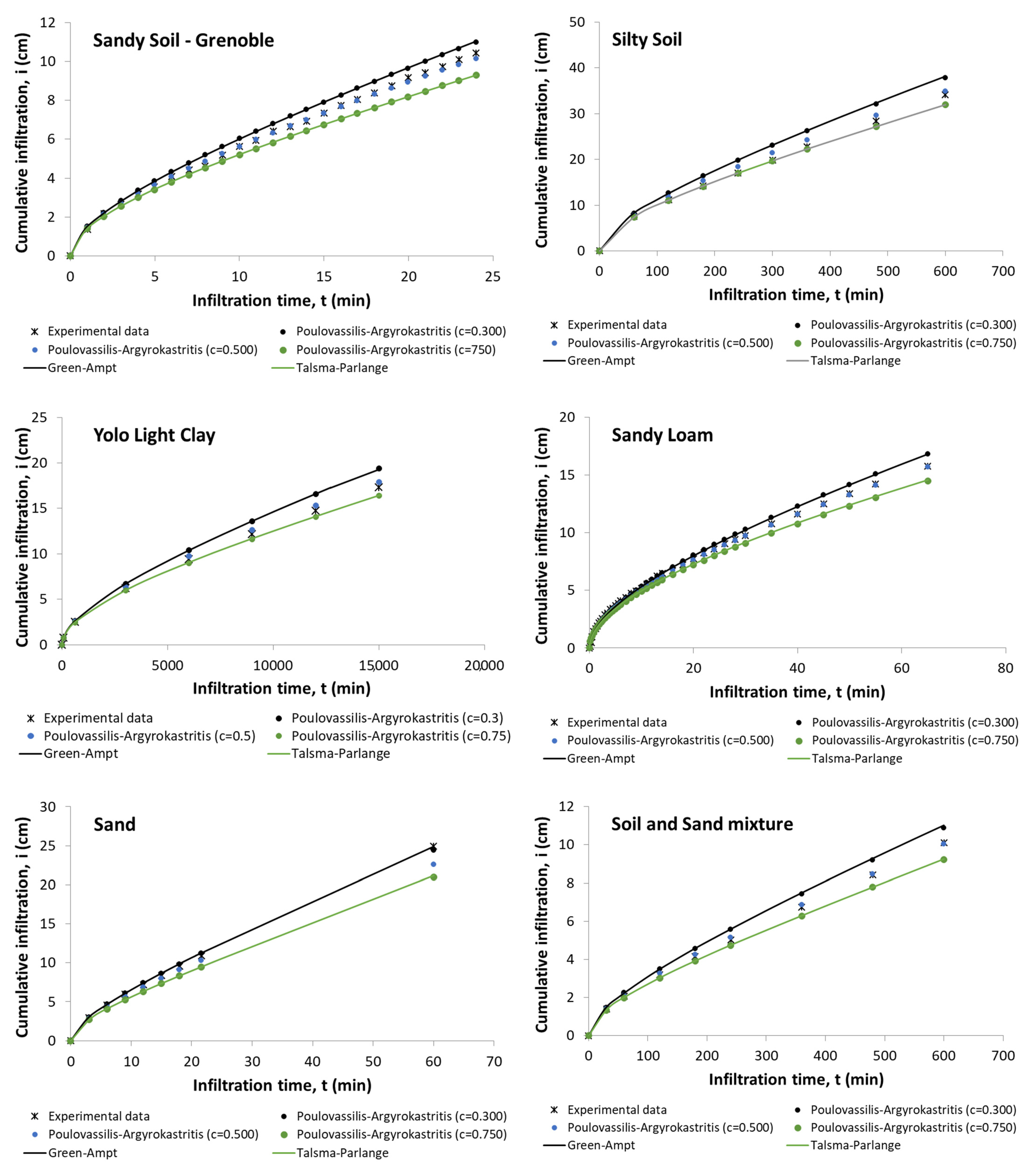
In Figure 1, a comparative presentation of the experimental relationship i(t) and the predicted ones according to equations of Talsma–Parlange, Green–Ampt, and Equation (1) for c = 0.300, 0.500 and 0.750 are depicted. As shown, for all soils studied, the i(t) values predicted from Equation (1) for c = 0.300 and c = 0.750 are almost the same with those calculated from the equations of Green–Ampt and Talsma–Parlange, respectively. Thus, the parameter c in real soils ranged from 0.300 to 0.750 and the two extreme values of the parameter c (0.300 and 0.750) correspond to the two extreme infiltration behavior soils described from the Green–Ampt equation (Equation (2)), which is characterized by the fact that the diffusivity function D(θ) approximates a delta function, and from the Talsma–Parlange equation (Equation (3)), where function D(θ) and dK/dθ change rapidly and are almost proportional [19]. Consequently, it is expected that the experimental relationship i(t) will be between these two limiting cases in each soil. Indeed, the experimental i(t) is always between these two limiting cases (Figure 1).

Next, the special case where the parameter c is fixed at 0.500 is studied and the Equation (1) is converted into the two-parameter Equation (6) as:

$$\mathrm{i}=\mathrm{S}\sqrt{\mathrm{t}}{\mathrm{e}}^{\left(-0.5\left(\frac{{\mathrm{K}}_{\mathrm{s}}}{\mathrm{S}}\right)\sqrt{\mathrm{t}}\right)}+{\mathrm{K}}_{\mathrm{s}}\mathrm{t}$$

(6)

As shown in Figure 1, the relationship i(t) predicted from Equation (6) (c = 0.500) is approximately located at the middle of the area defined by the two limiting cases. It could be assumed that the value of c = 0.500 is typically representative for the cumulative infiltration of many soils in the case of non-ponding conditions. Especially, this assumption could be useful for practical purposes since it helps to reliably predict i(t), which is explicit in terms of time. The accuracy of the i(t) predictions from Equation (6) was examined by the RMSE values for all soils studied. As shown in

Table 2. Root mean square error values (RMSE) of the predicted relationships i(t) from Equation (6) for all porous media studied.

Soil	RMSE (cm)
Sand	0.901
Soil and Sand Mixture	0.083
Sandy Soil-Grenoble	0.133
Silty Soil	1.126
Yolo Light Clay	0.405
Silty Loam GE3	0.302
Guelph Loam	0.327
Sandy Loam	0.166

, the RMSE values for all soils are small, which demonstrates that Equation (6) reliably predicts the relationship i(t).

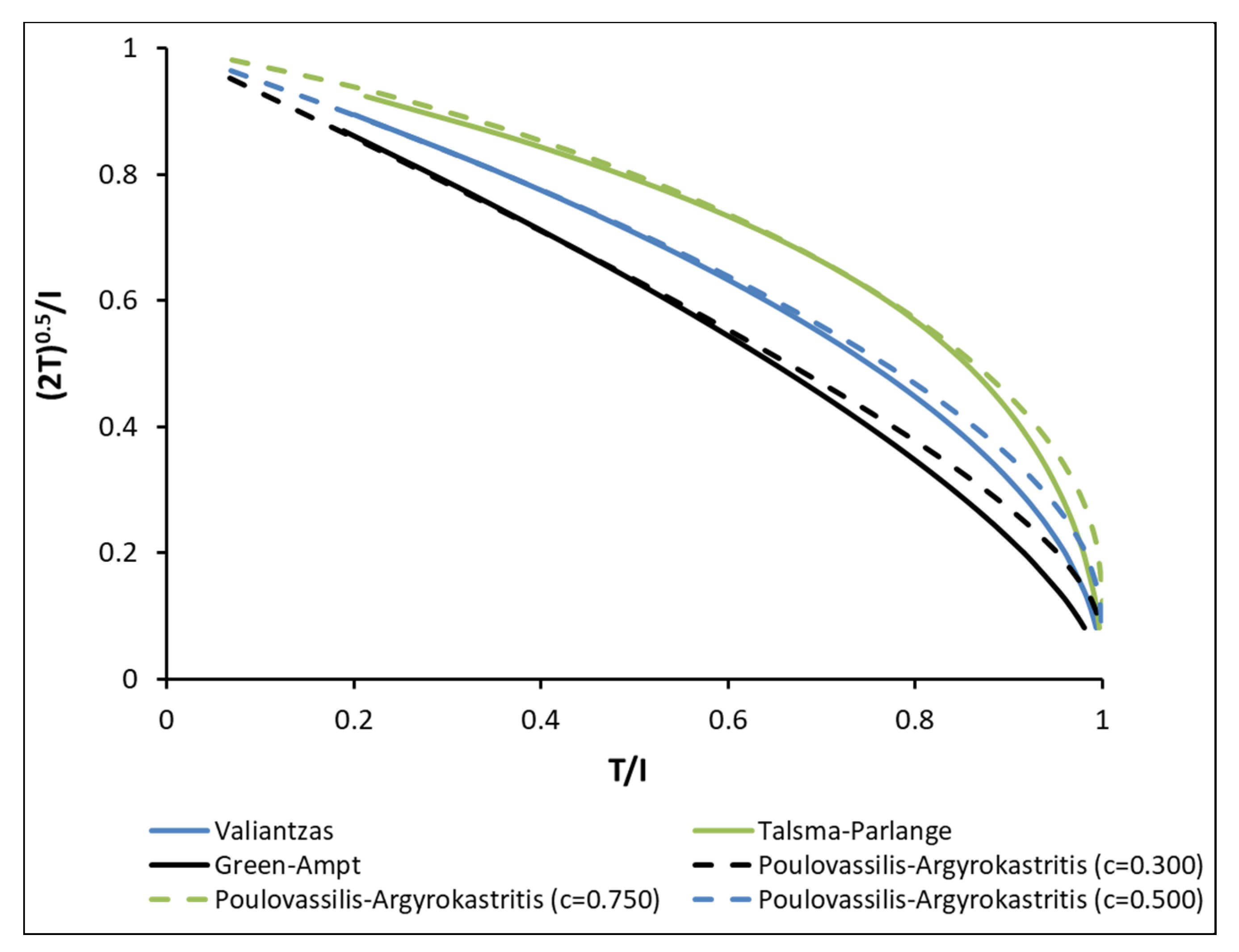
In order to enhance the above-mentioned results, we also applied the dimensionless variables of cumulative infiltration I and time T as defined by Valiantzas [25]

$$\mathrm{I}=2{\mathrm{K}}_{\mathrm{s}}\frac{\mathrm{i}}{{\mathrm{S}}^2}$$

(7)

$$\mathrm{T}=2{\mathrm{K}}_{\mathrm{s}}^2\frac{\mathrm{t}}{{\mathrm{S}}^2}$$

(8)

So, the dimensionless form of the Equation (1) is converted to

$$\mathrm{I}=\sqrt{2\mathrm{T}}{\mathrm{e}}^{-\mathrm{c}{\left(\frac{\mathrm{T}}{2}\right)}^{0.5}}+\mathrm{T}$$

(9)

In this case, the relative weighed effect of pressure head gradient in dimensionless form will be equal to (2T)^0.5/I, while the relative effect of gravity will be equal to T/I [15,25].

Figure 2 shows the relative weighed effect of pressure head gradient in dimensionless form (2T)^0.5/I as a function of T/I (relative effect of gravity) according to equations of Talsma–Parlange, Green–Ampt, Valiantzas, and Equation (9) for c = 0.300, 0.500, and 0.750. As shown, Equation (9) for c = 0.500 is approximately located at the middle of the area defined by the two extreme cases. For c values equal to 0.300 and 0.750, Equation (9) gives the same results with the Green–Ampt and Talsma–Parlange equations, respectively, while for c = 0.500, it gives the same results with the Valiantzas [25] equation. Small discrepancies exist between Green–Ampt equation and Equation (9) for c = 0.300, as well as between the Valiantzas equation and Equation (9) for c = 0.500, which are presented for T/I values greater than 0.8. Noting that these values correspond to T values greater than 6 and thus to very long infiltration time values. It is typically reported that for the Sandy Soil-Grenoble, the infiltration time for T = 6 corresponds to t = 80 min when the experimental duration of infiltration is 24 min.

3.2. Results from Non Linear Optimization for Estimation of K_s and S. Fixed c = 0.500 vs. Variable c Generated from Non Linear Optimization

As shown in

Table 3. Measured values of S and K_s and predicted values of S, K_s, and c from the Equation (1) using the Solver application considering (a) all the three parameters as adjustment parameters, and (b) the S and K_s as adjustment parameters and the c = 0.500. Relative errors (RE%) of the predicted values of S and K_s for all porous media studied.

Soil	Predicted Values (Equation (1) with Adjusted c)			Predicted Values (Equation (1) with Fixed c)			Measured Values
	S (cmmin−0.5)	Ks (cmmin−1)	c	S (cmmin−0.5)	Ks (cmmin−1)	c	S (cmmin−0.5)	Ks (cmmin−1)
Sand	1.505	0.369	0.752	1.342	0.352	0.500	1.375	0.3
Soil and Sand Mixture	0.241	0.014	0.907	0.209	0.013	0.500	0.223	0.012
Sandy Soil-Grenoble	1.375	0.337	0.881	1.224	0.294	0.500	1.319	0.255
Silty Soil	1.132	0.051	1.841	0.737	0.041	0.500	0.849	0.038
Yolo Light Clay	0.100	0.00079	0.826	0.093	0.00066	0.500	0.095	0.0007
Silty Loam GE3	0.311	0.0021	0.188	0.314	0.0030	0.500	0.316	0.0034
Guelph Loam	0.611	0.0206	0.580	0.603	0.0194	0.500	0.6181	0.0219
Sandy Loam	1.596	0.1432	0.939	1.513	0.097	0.500	1.445	0.11
	RE%
Sand	9.43	22.96		2.38	17.42
Soil and Sand Mixture	8.04	18.02		6.49	6.07
Sandy Soil-Grenoble	4.22	32.31		7.18	15.35
Silty Soil	33.29	33.41		13.25	8.05
Yolo Light Clay	4.85	12.18		2.57	5.64
Silty Loam GE3	1.56	39.53		0.77	12.53
Guelph Loam	1.19	6.01		2.37	11.53
Sandy Loam	10.46	30.17		4.71	11.96
Max |RE|=	33.29	39.53		13.25	17.42

, when the nonlinear optimization process was applied using the three adjustment parameters S, K_s, and c in Equation (1), the values of RE for S prediction ranged from 1.19% to 33.29% and for K_s from 6.01% to 39.53%. Generally, there is a tendency to overestimate S and underestimate K_s. The values of the parameter c ranged from 0.188 to 1.841. The maximum values of RE (33.29% and 39.53% for the Silty Soil and Silty Loam GE3, respectively) were observed at the extreme values of the parameter c.

Considering the scenario where the parameter c is fixed with value c = 0.500 and the two adjustment parameters are S and K_s, a significant improvement in the RE values was observed (Table 3). Specifically, the values for S ranged from 0.77 to 13.25% and for K_s from 5.64 to 17.42%. In all soil studied, the RE values for S are smaller than those for K_s. The relatively small values of RE for both parameters indicates that reliable predictions of S and K_s can be obtained with the help of the Solver tool when the third parameter is fixed at 0.500. As shown from the abovementioned, if the parameter c is used as an adjustment parameter it does not improve the predictions of the other two physical parameters (S, K_s). Therefore, it is proposed to apply the nonlinear optimization procedure using two adjustment parameters (S and K_s) and fixed the third parameter (c = 0.500). A similar phenomenon had occurred for the equation of Parlange et al. [19] and redefined by Haverkamp et al. [37], where the third parameter β was fixed at 0.6 [14,16,30,32]. The results of the nonlinear optimization procedure with two adjustment parameters are very good in the case of soils where the S/K_s ratio is very large, i.e., fine-textured soils [15]. For these soils, the values of S/K_s are 135.7, 93 and 28.22 for Yolo Light Clay, Silty Loam GE3, and Guelph Loam, respectively. In these cases, the RE values for S ranged from 0.77 to 2.57% and for K_s from 5.64 to 12.53%.

3.3. Assessment of K_s and S through Infiltration Time Using Non Linear Optimization

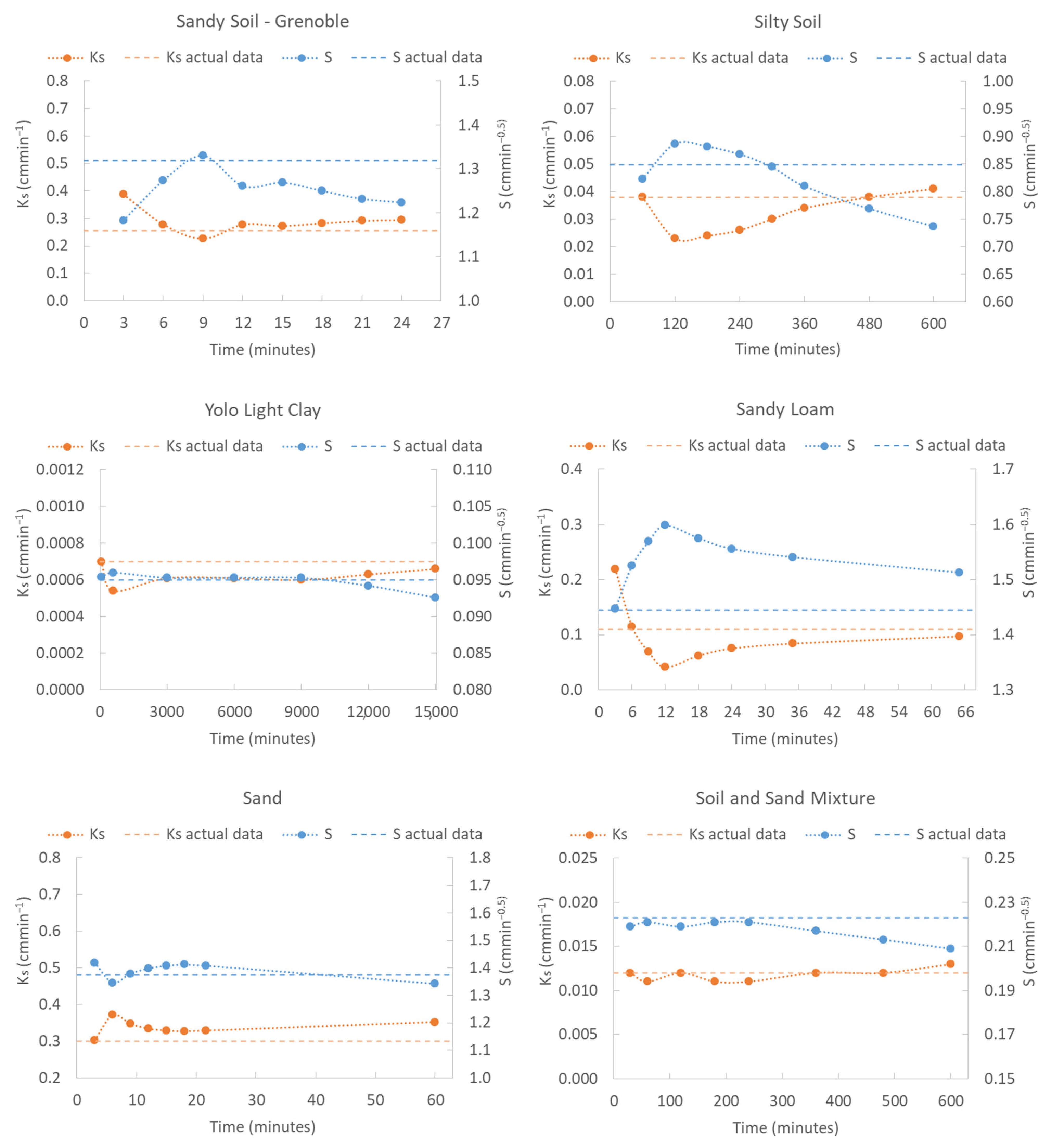
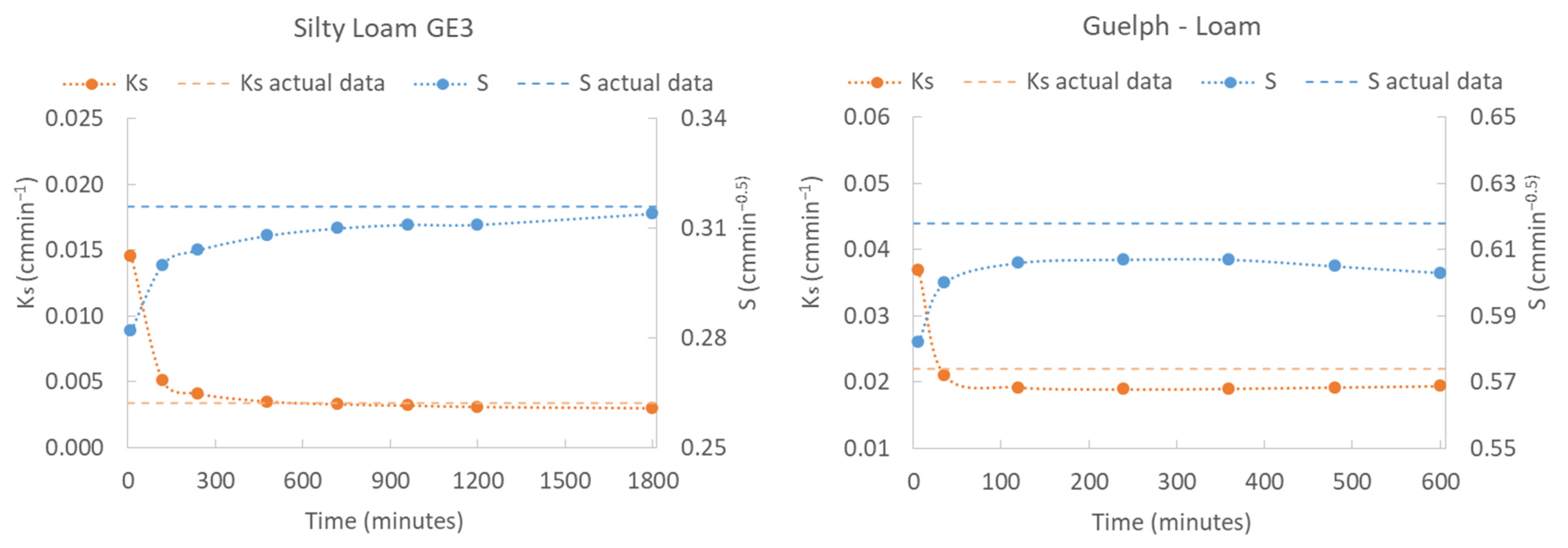
The accuracy of the Equation (1) in predicting S and K_s with respect to time was examined by considering the value of the parameter c as fixed (c = 0.500). Regarding K_s, the reliability of the prediction, generally, increases with time in all soils studied. In some soils (i.e., Sandy Soil-Grenoble, Guelph Loam, Silty Loam GE3 and Sandy Loam), an overestimation of K_s was observed at early times, but the accuracy of the prediction was significantly improved over time (Figure 3). It appears that relatively long infiltration times are required to best predict K_s (e.g., t > 40 min for Guelph Loam soil; t > 120 min for Silty Loam GE3).

As shown in Figure 3, a diverge of the predicted values of S after a specific infiltration time is observed in three of the soils studied (i.e., Sandy Soil-Grenoble, Silty Soil and Soil-Sand Mixture), while in the remaining soils, the predicted values are relatively stable.

It is also worth noting that the predictions of S and K_s are between those obtained from GA and TP equations that define the extreme infiltration limits of real soils.

3.4. The Equation of Infiltration Rate

Considering that the two-parameter Equation (6) can reliably predict the infiltration data i(t), the infiltration rate, u = di/dt, is expressed by the following useful explicit equation:

$$\mathrm{u}=0.5{\mathrm{e}}^{-0.5\left(\frac{{\mathrm{K}}_{\mathrm{s}}}{\mathrm{S}}\right)\sqrt{\mathrm{t}}}\left(\frac{\mathrm{S}}{\sqrt{\mathrm{t}}}-0.5{\mathrm{K}}_{\mathrm{s}}\right)+{\mathrm{K}}_{\mathrm{s}}$$

(10)

From Equation (10), when t→0 the u → ∞, whereas when t→∞ the u → K_s as this is expected from the physics of the phenomenon.

4. Conclusions

The equation of Poulovassilis and Argyrokastritis [17], which is an explicit equation of cumulative infiltration as function of time, is further investigated aiming at clarifying the parameter c used. It was found that for values of c = 0.300 and c = 0.750, it approaches the two extreme behavior infiltration models, the Green–Ampt and Talsma–Parlange. It is proposed for practical purposes to use it for c = 0.500 and thus it is converted into the two-parameter equation with S and K_s. This equation seems to have applicability in most soil types since the predicted i(t) relationships were very satisfactory. For this value of c, it gives almost the same results as the Valiantzas equation [25]. For the reliable estimation of S and K_s by applying the non-linear optimization procedure, the use of S and K_s as adjustment parameters and c as fixed at 0.500 is proposed. From the results, it appears that relatively long infiltration times are required for the best prediction of K_s.

References

- Mishra, S.K.; Kumar, S.R.; Singh, V.P. Calibration of a general infiltration model. Hydrol. Process. 1999, 13, 1691–1718. [Google Scholar] [CrossRef]
- Parhi, P.K.; Mishra, S.K.; Singh, R. A modification to Kostiakov and modified Kostiakov infiltration models. Water Resour. Manag. 2007, 21, 1973–1989. [Google Scholar] [CrossRef]
- Green, W.H.; Ampt, G.A. Studies on Soil Physics. J. Agric. Sci. 1911, 4, 1–24. [Google Scholar] [CrossRef]
- Philip, J.R. The theory of infiltration: 4. Sorptivity and algebraic infiltration equations. Soil Sci. 1957, 84, 257–264. [Google Scholar] [CrossRef]
- Philip, J.R. Theory of infiltration. Adv. Hydrosci. 1969, 5, 215–296. [Google Scholar]
- Swartzendruber, D. A quasi-solution of Richards’ equation for the downward infiltration of water into soil. Water Resour. Res. 1987, 23, 809–817. [Google Scholar] [CrossRef]
- Horton, R.I. The interpretation and application of runoff plot experiments with reference to soil erosion problems. Proc. Soil Sci. Soc. Am. 1938, 3, 340–349. [Google Scholar] [CrossRef]
- Holtan, H.N. A Concept of Infiltration Estimates in Watershed Engineering; URS41–41; US Department of Agriculture Service: Washington, DC, USA, 1961. [Google Scholar]
- Singh, V.P.; Yu, F.X. Derivation of infiltration equation using systems approach. J. Irrig. Drain. Eng. ASCE 1990, 116, 837–857. [Google Scholar] [CrossRef]
- Kostiakov, A.N. On the dynamics of the coefficients of water percolation in soils and on the necessity of studying it from a dynamic point of view for purposes of amelioration. Trans. 6th Commission. Int. Soc. Soil Sci. 1932, Part A, 15–21. [Google Scholar]
- Philip, J.R. The theory of infiltration: 6 Effect of water depth over soil. Soil Sci. 1958, 85, 278–286. [Google Scholar] [CrossRef]
- Haverkamp, R.; Kutilek, M.; Parlange, J.Y.; Rendon, L.; Krejca, M. Infiltration under ponded conditions: 2. infiltration equations tested for parameter time-dependence and predictive use. Soil Sci. 1988, 145, 317–329. [Google Scholar] [CrossRef]
- Poulovassilis, A.; Elmaloglou, S.; Kerkides, P.; Argyrokastritis, I. A variable sorptivity infiltration equation. Water Resour. Manag. 1989, 3, 287–298. [Google Scholar] [CrossRef]
- Rahmati, M.; Latorre, B.; Lassabatere, L.; Angulo-Jaramillo, R.; Moret-Fernández, D. The relevance of Philip theory to Haverkamp quasi-exact implicit analytical formulation and its uses to predict soil hydraulic properties. J. Hydrol. 2019, 570, 816–826. [Google Scholar] [CrossRef]
- Kargas, G.; Londra, P.A. Comparison of two-parameter vertical ponded infiltration equations. Environ. Model. Assess. 2021, 26, 179–186. [Google Scholar] [CrossRef]
- Kargas, G.; Koka, D.; Londra, P.A. Determination of Soil Hydraulic Properties from Infiltration Data Using Various Methods. Land 2022, 11, 779. [Google Scholar] [CrossRef]
- Poulovassilis, A.; Argyrokastritis, I. A new approach for studying vertical infiltration. Soil Res. 2020, 58, 509–518. [Google Scholar] [CrossRef]
- Brutsaert, W. Vertical infiltration in dry soil. Water Resour. Res. 1977, 13, 363–368. [Google Scholar] [CrossRef]
- Parlange, J.Y.; Lisle, I.; Braddock, R.D.; Smith, R.E. The three-parameter infiltration equation. Soil Sci. 1982, 133, 337–341. [Google Scholar] [CrossRef]
- Talsma, T.; Parlange, J.-Y. One-dimensional vertical infiltration. Aust. J. Soil Res. 1972, 10, 143. [Google Scholar] [CrossRef]
- Vrugt, J.A.; Gao, Y. On the three-parameter infiltration equation of Parlange et al. (1982): Numerical solution, experimental design, and parameter estimation. Vadose Zone J. 2022, 21, e20167. [Google Scholar] [CrossRef]
- Rahmati, M.; Vanderborght, J.; Simunek, J.; Vrugt, J.A.; Moret-Fernández, D.; Latorre, B.; Lassabatere, L.; Vereecken, H. Soil hydraulic properties estimation from one-dimensional infiltration experiments using characteristic time concept. Vadose Zone J. 2020, 19, e20068. [Google Scholar] [CrossRef]
- Smiles, D.E.; Knight, J.H. Anote on the use of the Philip infiltration equation. Aust. J. Soil Res. 1976, 14, 103–108. [Google Scholar] [CrossRef]
- Vandervaere, J.P.; Vauclin, M.; Elrick, D.E. Transient flow from tension infiltrometers: II. Four methods to determine sorptivity and conductivity. Soil Sci. Soc. Am. J. 2000, 64, 1272–1284. [Google Scholar] [CrossRef]
- Valiantzas, J.D. New linearized two-parameter infiltration equation for direct determination of conductivity and sorptivity. J. Hydrol. 2010, 384, 1–13. [Google Scholar] [CrossRef]
- Šimůnek, J.; Van Genuchten, M.T. Estimating unsaturated soil hydraulic properties from tension disc infiltrometer data by numerical inversion. Water Resour. Res. 1996, 32, 2683–2696. [Google Scholar] [CrossRef]
- Šimůnek, J.; Angulo-Jaramillo, R.; Schaap, M.G.; Vandervaere, J.P.; Van Genuchten, M.T. Using an inverse method to estimate the hydraulic properties of crusted soils from tension-disc infiltrometer data. Geoderma 1998, 86, 61–81. [Google Scholar] [CrossRef]
- Simunek, J.; Hopmans, J.W. Parameter Optimisation and Nonlinear Fitting. In Methods of Soil Analysis, 3rd ed.; Dane, J.H., Topp, G.C., Eds.; Part 1, Physical Methods; SSSA: Madison, WI, USA, 2002; Chapter 1.7. [Google Scholar]
- Lassabatere, L.; Angulo-Jaramillo, R.; Soria-Ugalde, J.M.; Šimůnek, J.; Haverkamp, R. Numerical evaluation of a set of analytical infiltration equations. Water Resour. Res. 2009, 45, W12415. [Google Scholar] [CrossRef]
- Latorre, B.; Peña, C.; Lassabatere, L.; Angulo-Jaramillo, R.; Moret-Fernández, D. Estimate of soil hydraulic properties from disc infiltrometer three-dimensional infiltration curve. Numerical analysis and field application. J. Hydrol. 2015, 527, 1–12. [Google Scholar] [CrossRef]
- Clothier, B.E.; Scotter, D. Unsaturated water transmission parameters obtained from infiltration. In Methods of Soil Analysis: Part 4; Dane, J.H., Topp, G.C., Eds.; Physical Methods, SSSA Book Series 5; SSSA: Madison, WI, USA, 2002; pp. 879–888. [Google Scholar]
- Latorre, B.; Moret-Fernández, D.; Lassabatere, L.; Rahmati, M.; López, M.V.; Angulo-Jaramillo, R.; Sorando, R.; Comin, F.; Jiménez, J.J. Influence of the β parameter of the Haverkamp model on the transient soil water infiltration curve. J. Hydrol. 2018, 564, 222–229. [Google Scholar] [CrossRef]
- van Genuchten, M.T. A closed-form equation for predicting the hydraulic conductivity of unsaturated soils. Soil Sci. Soc. Am. J. 1980, 44, 892–898. [Google Scholar] [CrossRef]
- Mualem, Y. A new model for predicting the hydraulic conductivity of unsaturated porous media. Water Resour. Res. 1976, 12, 513–522. [Google Scholar] [CrossRef]
- Wraith, J.M.; Or, D. Nonlinear parameter estimation using spreadsheet software. J. Nat. Resour. Life Sci. Educ. 1998, 27, 13–19. [Google Scholar] [CrossRef]
- Lasdon, L.S.; Fox, R.L.; Ratner, M.W. Nonlinear optimization using the generalized reduced gradient method. Revue française d’automatique, informatique, recherche opérationnelle. Rech. Opérationnelle 1974, 8, 73–103. [Google Scholar] [CrossRef]
- Haverkamp, R.; Parlange, J.Y.; Starr, J.L.; Schmitz, G.; Fuentes, C. Infiltration under ponded conditions: 3. A predictive equation based on physical parameters. Soil Sci. 1990, 149, 292–300. [Google Scholar] [CrossRef]
Figure 1.
Comparative presentation of the experimental relationship i(t) and the predicted ones according to equations of Talsma–Parlange, Green–Ampt, and Poulovassilis–Argyrokastritis (Equation (1) for c = 0.300, 0.500, and 0.750).
Figure 2.
The relative weighed effect of pressure head gradient in dimensionless form (2T)0.5/I as a function of T/I (relative weighed effect of gravity) according to equations of Green–Ampt, Talsma–Parlange, Valiantzas, and Poulovassilis–Argyrokastritis (Equation (9) for c = 0.300, 0.500 and 0.750).
Figure 3.
Measured Ks and S values and the predicted ones from Equation (6), with respect to the time, for all porous media studied.