Extreme Events Analysis Using LH-Moments Method and Quantile Function Family

Anghel, Cristian Gabriel; Stanca, Stefan Ciprian; Ilinca, Cornel

doi:10.3390/hydrology10080159

Open AccessArticle

Extreme Events Analysis Using LH-Moments Method and Quantile Function Family

by

Cristian Gabriel Anghel

^*

,

Stefan Ciprian Stanca

^*

and

Cornel Ilinca

^*

Faculty of Hydrotechnics, Technical University of Civil Engineering Bucharest, Lacul Tei, Nr.122–124, 020396 Bucharest, Romania

^*

Authors to whom correspondence should be addressed.

Hydrology 2023, 10(8), 159; https://0-doi-org.brum.beds.ac.uk/10.3390/hydrology10080159

Submission received: 29 June 2023 / Revised: 27 July 2023 / Accepted: 27 July 2023 / Published: 30 July 2023

(This article belongs to the Special Issue Climate Change Effects on Hydrology and Water Resources)

Download

Browse Figures

Versions Notes

Abstract

:

A direct way to estimate the likelihood and magnitude of extreme events is frequency analysis. This analysis is based on historical data and assumptions of stationarity, and is carried out with the help of probability distributions and different methods of estimating their parameters. Thus, this article presents all the relations necessary to estimate the parameters with the LH-moments method for the family of distributions defined only by the quantile function, namely, the Wakeby distribution of 4 and 5 parameters, the Lambda distribution of 4 and 5 parameters, and the Davis distribution. The LH-moments method is a method commonly used in flood frequency analysis, and it uses the annual series of maximum flows. The frequency characteristics of the two analyzed methods, which are both involved in expressing the distributions used in the first two linear moments, as well as in determining the confidence interval, are presented. The performances of the analyzed distributions and the two presented methods are verified in the following maximum flows, with the Bahna river used as a case study. The results are presented in comparison with the L-moments method. Following the results obtained, the Wakeby and Lambda distributions have the best performances, and the LH-skewness and LH-kurtosis statistical indicators best model the indicators’ values of the sample (0.5769, 0.3781, 0.548 and 0.3451). Similar to the L-moments method, this represents the main selection criterion of the best fit distribution.

Keywords:

extreme events; frequency analysis; flood; quantile function; Wakeby; Lambda; Davis; linear moments; higher order linear moments; Pareto; Tukey

1. Introduction

In flood frequency analysis (FFA), the main goal is to calculate the maximum flow corresponding to the area of low probability, where there are usually no records. In general, this analysis can be performed using the Annual Maximum Series (AMS) or Partial Series (Peak Over Thresholds or the Annual Exceedance Series).

In FFA using AMS, an important aspect is representing the observance of the “separation effect”, introduced by Matalas [1], which consists of reducing as much as possible the influence of the small values of the maximum flow, knowing that, in the annual series of maximum flows, they do not always represent flood flows. The advantages and disadvantages of using AMS and PS were presented in previous materials [2].

This research is part of a holistic analysis regarding the probability distributions and estimation methods of their parameters, according to the hydrological and hydrometric characteristics in Romania, taking into account climate change, which amplifies extreme events. This research is a proposal for the future normative for determining the maximum flows, in which there is the applicability of some families of distributions, including the Gamma family (Pearson 3, Log–Pearson, Wilson–Hilferty, Pseudo–Weibull, Chi, Inverse Chi, Pearson V, Krtisky–Menkel) [3,4], the GEV family (Fréchet, Weibull) [5], the generalized Pareto family [1], the generalized beta families [6,7] and the family of quantile functions (Wakeby, Lambda) [4,6].

The “separation effect” of the maximum flow can be achieved by using the distributions introduced in the FFA, especially the LH-moments method or the simultaneous use of multiple distributions, as is the case with this article.

The LH-moments method is a parameter estimation method, introduced by Wang [8], that analyzes the generalized distribution of extreme values and was popularized by Sharwar et al. [9], who formulated the LH-moments for five distributions, namely, Mielke–Johnson’s kappa distribution, the three–parameter kappa type II distribution, Beta–k distribution, Beta–p distribution and the generalized Gumbel distribution. Compared to the L-moments method, the LH-moments method has the advantage of assigning a lower importance to small extreme values (right hand, high exceedance probabilities) which do not always represent floods. This also represents the main disadvantage of using the Annual Maximum Series. In general, the LH-moments method can be applied up to level 4, but in this article, only the first two levels are analyzed because the use of the last two levels would constitute a very large deviation from the L-moments method, which is nevertheless a stable and robust method.

In frequency analysis, the LH-moments method was used frequently for low–flow frequency analysis [10], FFA [8,11,12,13], regional flood frequency analysis [14,15,16,17,18,19,20,21,22,23,24,25] and for the frequency analysis of the annual maximum rainfall series [26,27,28].

Regarding the distributions that naturally achieve a “separation effect”, one of the most used probability distributions for achieving this “separation effect” in FFA without sample censoring is the Wakeby distribution [1,4,29]. This was introduced in the analysis of annual maximum flows (without sample censoring) by Houghton [1], precisely to fulfill this principle, having as a particular case the four-parameter Wakeby distribution [29,30,31] and generalized Pareto distribution type II [4,29], the latter being the usual distribution applied in the case of frequency analysis using partial series (with sample censoring) [2,29,32,33]. Since 1978, the Wakeby distribution has been used for flood and regional flood frequency analysis [4,29,32,34,35,36], low–flow frequency analysis [6,37] and annual maximum rainfall analysis [38,39,40]. Using the LH-moments method, it was applied in various materials [41,42,43].

Other distributions that can achieve this “separation effect” but receive limited attention are the generalized Lambda distribution and the Davis distribution. The five parameters generalized Lambda distribution was generally used alongside the method of weighted moments and the method of linear moments [30]. In [6], it was applied for the first time for FFA using the method of ordinary moments (MOM), and all mathematical relations for parameter estimation using this method are being presented. It is a distribution that has as special cases, the four–parameter Lambda distribution and the three–parameter Tukey distribution [30].

Regarding the Lambda distribution and Davis distribution, they are for the first time applied for flood frequency analysis using the LH-moments method. Moreover, for the first time, the Davis distribution is applied using the L-moments method, and the relations for estimating the distribution parameters using the L-moments method are presented.

The purpose of the article is to present all the mathematical equations to apply the analyzed models, using both the L-moments method and the LH-moments method for parameter estimation. We also want to highlight the particular cases of these distributions, which under certain conditions turn into distributions usually applied in these types of analyses.

The performance of the proposed models and methods is examined, and an FFA is carried out for the Bahna River, Romania. The analysis is based on historical data and assumptions of stationarity. Because of climate change, the assumption that future conditions will be similar to those of the past may lose its validity. Selecting the best model is based on the L-moments and LH-moments values and diagrams.

2. Methods

Five distributions are analyzed that are part of the family of probability distributions and defined only by the inverse function, with applicability in FFA.

All the elements required to apply these distributions are presented, including the inverse function and the relations for estimating the parameters.

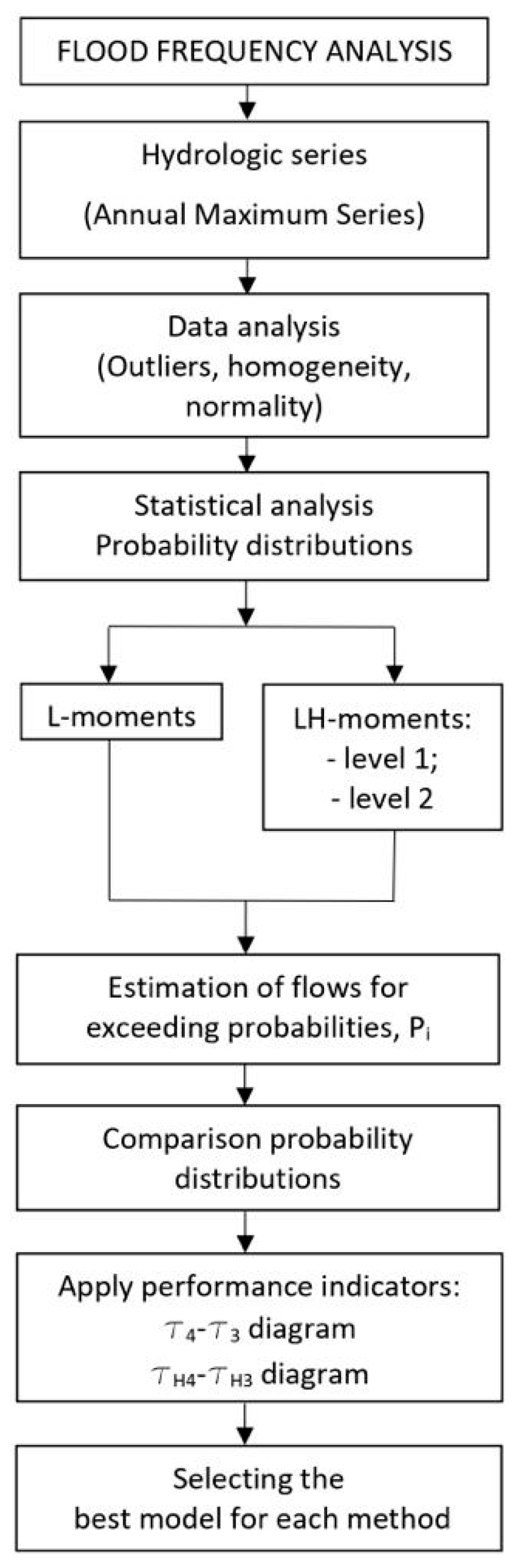
The analysis of the maximum flows for the Bahna River is carried out in stages, according to the flow chart presented in Figure 1. No outliers were detected (Grubb’s test). The series is homogeneous and the verification was completed with the von Neumann test [44]. To check the homogeneity, MASH v3.03 software can also be used, which was successfully applied in the area of the Pannonian basin [45].

2.1. Quantile Functions

In the section below, the analyzed probability distributions are presented. Distributions are defined only by the quantile function. The characteristic frequency factors of the two methods are highlighted in Appendix A.

-: The five-parameter Wakeby distribution (WK5) [1,4,29,30]:

x (p) = ξ + \frac{α}{β} \cdot (1 - p^{β}) - \frac{γ}{δ} \cdot (1 - p^{- δ})

(1)

where

ξ

represents the position parameter;

α

and

γ

represent the scale parameters; and

β

and

δ

represent the shape parameters.

-: The four-parameter Wakeby distribution (WK4) [4,29]:

x (p) = \frac{α}{β} \cdot (1 - p^{β}) - \frac{γ}{δ} \cdot (1 - p^{- δ})

(2)

-: The five-parameter Lambda distribution (L5) [30]:

x (p) = γ + α \cdot p^{β} - λ \cdot {(1 - p)}^{δ}

(3)

where

γ

represents the position parameter;

α

and

λ

represent the scale parameters; and

β

and

δ

represent the shape parameters.

-: The four-parameter Lambda distribution (L4):

x (p) = α \cdot p^{β} - λ \cdot {(1 - p)}^{δ}

(4)

-: The Davis distribution (DV) [46]:

x (p) = γ \cdot \frac{p^{α}}{{(1 - p)}^{λ}}

(5)

where

γ

represents the scale parameter, and

α

and

λ

represent the shape parameters.

2.2. The L- and LH-Moments Estimations Equations

The methods are the L- and LH-moments. The sample L-moments and LH-moments are determined according to [29,30,31,32], respectively [1]. Only the first and second order LH-moments are analyzed.

The relationship between L-moments and LH-moments are presented in Appendix B.

2.2.1. The Five-Parameter Wakeby Distribution (WK5)

The L-moments estimations equations can be expressed as [4,29,30,31,32]:

L_{1} = ξ + \frac{α}{β + 1} + \frac{γ}{1 - δ}

(6)

L_{2} = \frac{α}{(β + 1) \cdot (β + 2)} + \frac{γ}{(2 - δ) \cdot (1 - δ)}

(7)

L_{3} = \frac{γ \cdot (δ + 1)}{(1 - δ) \cdot (2 - δ) \cdot (3 - δ)} + \frac{α \cdot (1 - β)}{(β + 1) \cdot (β + 2) \cdot (β + 3)}

(8)

L_{4} = \frac{γ \cdot (δ + 1) \cdot (δ + 2)}{(4 - δ) \cdot (3 - δ) \cdot (2 - δ) \cdot (1 - δ)} + \frac{α \cdot (2 - β) \cdot (1 - β)}{(β + 1) \cdot (β + 2) \cdot (β + 3) \cdot (β + 4)}

(9)

where

L_{1}, L_{2}, L_{3}, L_{4}

represents the first four linear moments.

The first order LH-moments estimations equations:

L_{H 1} = \frac{ξ \cdot (β^{2} + 3 \cdot β + 2) + α \cdot β + 3 \cdot α}{(β + 1) \cdot (β + 2)} - \frac{γ \cdot (δ - 3)}{(δ - 2) \cdot (δ - 1)}

(10)

L_{H 2} = \frac{3 \cdot α}{(β + 1) \cdot (β + 2) \cdot (β + 3)} - \frac{3 \cdot γ}{(δ - 3) \cdot (δ - 2) \cdot (δ - 1)}

(11)

L_{H 3} = \frac{4 \cdot γ \cdot (δ + 1)}{(δ - 4) \cdot (δ - 3) \cdot (δ - 2) \cdot (δ - 1)} - \frac{4 \cdot α \cdot (β - 1)}{(β + 1) \cdot (β + 2) \cdot (β + 3) \cdot (β + 4)}

(12)

L_{H 4} = \frac{5 \cdot γ \cdot (δ + 1) \cdot (δ + 2)}{(δ - 5) \cdot (δ - 4) \cdot (δ - 3) \cdot (δ - 2) \cdot (δ - 1)} + \frac{5 \cdot α \cdot (β - 2) \cdot (β - 1)}{(β + 1) \cdot (β + 2) \cdot (β + 3) \cdot (β + 4) \cdot (β + 5)}

(13)

where

L_{H 1}, L_{H 2}, L_{H 3}, L_{H 4}

represents the first four LH-moments.

The second order LH-moments estimations equations:

L_{H 1} = \frac{ξ \cdot (β^{3} + 6 \cdot β^{2} + 11 \cdot β + 6) + α \cdot β^{2} + 6 \cdot α \cdot β + 11 \cdot α}{(β + 1) \cdot (β + 2) \cdot (β + 3)} - \frac{γ \cdot (δ^{2} - 6 \cdot δ + 11)}{(δ - 3) \cdot (δ - 2) \cdot (δ - 1)}

(14)

L_{H 2} = \frac{12 \cdot α}{(β + 1) \cdot (β + 2) \cdot (β + 3) \cdot (β + 4)} + \frac{12 \cdot γ}{(δ - 4) \cdot (δ - 3) \cdot (δ - 2) \cdot (δ - 1)}

(15)

L_{H 3} = - \frac{20 \cdot γ \cdot (δ + 1)}{(δ - 5) \cdot (δ - 4) \cdot (δ - 3) \cdot (δ - 2) \cdot (δ - 1)} - \frac{20 \cdot α \cdot (β - 1)}{(β + 1) \cdot (β + 2) \cdot (β + 3) \cdot (β + 4) \cdot (β + 5)}

(16)

L_{H 4} = \frac{30 \cdot γ \cdot (δ + 1) \cdot (δ + 2)}{(δ - 6) \cdot (δ - 5) \cdot (δ - 4) \cdot (δ - 3) \cdot (δ - 2) \cdot (δ - 1)} + \frac{30 \cdot α \cdot (β - 2) \cdot (β - 1)}{(β + 1) \cdot (β + 2) \cdot (β + 3) \cdot (β + 4) \cdot (β + 5) \cdot (β + 6)}

(17)

2.2.2. The Four-Parameter Wakeby Distribution (WK4)

Parameter estimations of the L-moments [29]:

L_{1} = \frac{α}{β + 1} - \frac{γ}{δ - 1}

(18)

L_{2} = \frac{α}{(β + 1) \cdot (β + 2)} + \frac{γ}{(δ - 2) \cdot (δ - 1)}

(19)

L_{3} = - \frac{γ \cdot (δ + 1)}{(δ - 3) \cdot (δ - 2) \cdot (δ - 1)} - \frac{α \cdot (β - 1)}{(β + 1) \cdot (β + 2) \cdot (β + 3)}

(20)

L_{4} = \frac{α \cdot (β - 2) \cdot (β - 1)}{(β + 1) \cdot (β + 2) \cdot (β + 3) \cdot (β + 4)} - \frac{γ \cdot (δ + 1) \cdot (δ + 2)}{(δ - 4) \cdot (δ - 3) \cdot (δ - 2) \cdot (δ - 1)}

(21)

The first order LH-moments estimations equations:

L_{H 1} = \frac{α \cdot (β + 3)}{(β + 1) \cdot (β + 2)} - \frac{γ \cdot (δ - 3)}{(δ - 2) \cdot (δ - 1)}

(22)

For linear moments

L_{H 2}, L_{H 3}, L_{H 4}

, the relations are the same as in the WK5 distribution.

The second order LH-moments estimations equations:

L_{H 1} = \frac{α \cdot (β^{2} + 6 \cdot β^{2} + 11) + α \cdot β^{2} + 6 \cdot α \cdot β + 11 \cdot α}{(β + 1) \cdot (β + 2) \cdot (β + 3)} - \frac{γ \cdot (δ^{2} - 6 \cdot δ + 11)}{(δ - 3) \cdot (δ - 2) \cdot (δ - 1)}

(23)

For linear moments

L_{H 2}, L_{H 3}, L_{H 4}

, the relations are the same as in the WK5 distribution.

2.2.3. The Five-Parameter Lambda Distribution (L5)

Parameter estimation of the L-moments:

L_{1} = \frac{γ \cdot (β + 1) + α}{β + 1} - \frac{λ}{δ + 1}

(24)

L_{2} = - \frac{α \cdot β}{(β + 1) \cdot (β + 2)} - \frac{λ \cdot δ}{(δ + 1) \cdot (δ + 2)}

(25)

L_{3} = \frac{α \cdot β \cdot (β - 1)}{(β + 1) \cdot (β + 2) \cdot (β + 3)} + \frac{λ \cdot δ \cdot (1 - δ)}{(δ + 1) \cdot (δ + 2) \cdot (δ + 3)}

(26)

L_{4} = \frac{λ \cdot δ \cdot (3 \cdot δ - δ^{2} - 2)}{(δ + 1) \cdot (δ + 2) \cdot (δ + 3) \cdot (δ + 4)} - \frac{α \cdot β \cdot (β - 2) \cdot (β - 1)}{(β + 1) \cdot (β + 2) \cdot (β + 3) \cdot (β + 4)}

(27)

The first order LH-moments estimations equations:

L_{H 1} = \frac{γ \cdot (β^{2} + 3 \cdot β + 2) + 2 \cdot α}{(β + 1) \cdot (β + 2)} - \frac{2 \cdot λ}{δ + 2}

(28)

L_{H 2} = - \frac{3 \cdot α \cdot β}{(β + 1) \cdot (β + 2) \cdot (β + 3)} - \frac{3 \cdot δ \cdot λ}{2 \cdot (δ + 2) \cdot (δ + 3)}

(29)

L_{H 3} = \frac{4 \cdot α \cdot β \cdot (β - 1)}{(β + 1) \cdot (β + 2) \cdot (β + 3) \cdot (β + 4)} - \frac{4 \cdot δ \cdot λ \cdot (δ - 1)}{3 \cdot (δ + 4) \cdot (δ + 3) \cdot (δ + 2)}

(30)

L_{H 4} = - \frac{5 \cdot α \cdot β \cdot (β - 2) \cdot (β - 1)}{(β + 1) \cdot (β + 2) \cdot (β + 3) \cdot (β + 4) \cdot (β + 5)} - \frac{5 \cdot δ \cdot λ \cdot (δ - 1) \cdot (δ - 2)}{4 \cdot (δ + 5) \cdot (δ + 4) \cdot (δ + 3) \cdot (δ + 2)}

(31)

The second order LH-moments estimations equations:

L_{H 1} = \frac{γ \cdot (β^{3} + 6 \cdot β^{2} + 11 \cdot β + 6) + 6 \cdot α}{(β + 1) \cdot (β + 2) \cdot (β + 3)} - \frac{3 \cdot λ}{δ + 3}

(32)

L_{H 2} = - \frac{12 \cdot α \cdot β}{(β + 1) \cdot (β + 2) \cdot (β + 3) \cdot (β + 4)} - \frac{2 \cdot δ \cdot λ}{(δ + 3) \cdot (δ + 4)}

(33)

L_{H 3} = \frac{20 \cdot α \cdot β \cdot (β - 1)}{(β + 1) \cdot (β + 2) \cdot (β + 3) \cdot (β + 4) \cdot (β + 5)} - \frac{5 \cdot δ \cdot λ \cdot (δ - 1)}{3 \cdot (δ + 5) \cdot (δ + 4) \cdot (δ + 3)}

(34)

L_{H 4} = - \frac{30 \cdot α \cdot β \cdot (β - 2) \cdot (β - 1)}{(β + 1) \cdot (β + 2) \cdot (β + 3) \cdot (β + 4) \cdot (β + 5) \cdot (β + 6)} - \frac{3 \cdot δ \cdot λ \cdot (δ - 1) \cdot (δ - 2)}{2 \cdot (δ + 6) \cdot (δ + 5) \cdot (δ + 4) \cdot (δ + 3)}

(35)

2.2.4. The Four-Parameter Lambda Distribution (L4)

Parameter estimation of the L-moments:

L_{1} = \frac{α}{β + 1} - \frac{λ}{δ + 1}

(36)

L_{2} = - \frac{α \cdot β}{(β + 1) \cdot (β + 2)} - \frac{λ \cdot δ}{(δ + 1) \cdot (δ + 2)}

(37)

L_{3} = \frac{α \cdot β \cdot (β - 1)}{(β + 1) \cdot (β + 2) \cdot (β + 3)} + \frac{λ \cdot δ \cdot (1 - δ)}{(δ + 1) \cdot (δ + 2) \cdot (δ + 3)}

(38)

L_{4} = \frac{λ \cdot δ \cdot (δ - 2) \cdot (δ - 1)}{(δ + 1) \cdot (δ + 2) \cdot (δ + 3) \cdot (δ + 4)} - \frac{α \cdot β \cdot (β - 2) \cdot (β - 1)}{(β + 1) \cdot (β + 2) \cdot (β + 3) \cdot (β + 4)}

(39)

The first order LH-moments estimations equations:

L_{H 1} = \frac{2 \cdot α}{(β + 1) \cdot (β + 2)} - \frac{2 \cdot λ}{δ + 2}

(40)

For linear moments

L_{H 2}, L_{H 3}, L_{H 4}

, the relations are the same as in the L5 distribution.

The second order LH-moments estimations equations:

L_{H 1} = \frac{6 \cdot α}{(β + 1) \cdot (β + 2) \cdot (β + 3)} - \frac{3 \cdot λ}{δ + 3}

(41)

For linear moments

L_{H 2}, L_{H 3}, L_{H 4}

, the relations are the same as in the L5 distribution.

2.2.5. Davis Distribution (DV)

Parameter estimation of the L-moments:

L_{1} = γ \cdot \frac{Γ (α + 1) \cdot (1 - λ)}{Γ (α + 2 - λ)}

(42)

L_{2} = \frac{γ \cdot α \cdot π \cdot Γ (α) \cdot (λ + α)}{Γ (α - λ) \cdot (λ - α - 2) \cdot (λ - α - 1) \cdot (λ - α) \cdot Γ (λ) \cdot \sin (λ \cdot π)}

(43)

L_{3} = \frac{γ \cdot α \cdot π \cdot Γ (α) \cdot (λ^{2} + λ \cdot (4 \cdot α + 1) + α^{2} - α)}{Γ (α - λ) \cdot (λ - α - 3) \cdot (λ - α - 2) \cdot (λ - α - 1) \cdot (λ - α) \cdot Γ (λ) \cdot \sin (λ \cdot π)}

(44)

The first order LH-moments estimations equations:

L_{H 1} = 2 \cdot γ \cdot \frac{Γ (α + 1) \cdot (2 - λ)}{Γ (α + 3 - λ)}

(45)

L_{H 2} = \frac{3 \cdot γ \cdot α \cdot π \cdot Γ (α) \cdot (λ + 2 \cdot α) \cdot (λ - 1)}{Γ (α - λ) \cdot 2 \cdot (λ - α - 3) \cdot (λ - α - 2) \cdot (λ - α - 1) \cdot (λ - α) \cdot Γ (λ) \cdot \sin (λ \cdot π)}

(46)

L_{H 3} = \frac{4 \cdot γ \cdot α \cdot π \cdot Γ (α) \cdot (λ - 1) \cdot (λ^{2} + λ \cdot (6 \cdot α + 1) + 3 \cdot α^{2} - 3 \cdot α)}{Γ (α - λ) \cdot 3 \cdot (λ - α - 4) \cdot (λ - α - 3) \cdot (λ - α - 2) \cdot (λ - α - 1) \cdot (λ - α) \cdot Γ (λ) \cdot \sin (λ \cdot π)}

(47)

The second order LH-moments estimations equations:

L_{H 1} = 3 \cdot γ \cdot \frac{Γ (α + 1) \cdot (3 - λ)}{Γ (α - λ + 4)}

(48)

L_{H 2} = \frac{2 \cdot γ \cdot α \cdot π \cdot Γ (α) \cdot (λ + 3 \cdot α) \cdot (λ - 2) \cdot (λ - 1)}{Γ (α - λ) \cdot (λ - α - 4) \cdot (λ - α - 3) \cdot (λ - α - 2) \cdot (λ - α - 1) \cdot (λ - α) \cdot Γ (λ) \cdot \sin (λ \cdot π)}

(49)

L_{H 3} = \frac{5 \cdot γ \cdot α \cdot π \cdot Γ (α) \cdot (λ - 2) \cdot (λ - 1) \cdot (λ^{2} + λ \cdot (8 \cdot α + 1) + 6 \cdot α^{2} - 6 \cdot α)}{Γ (α - λ) \cdot 3 \cdot (λ - α - 5) \cdot (λ - α - 4) \cdot (λ - α - 3) \cdot (λ - α - 2) \cdot (λ - α - 1) \cdot (λ - α) \cdot Γ (λ) \cdot \sin (λ \cdot π)}

(50)

3. Study Area and Main Data

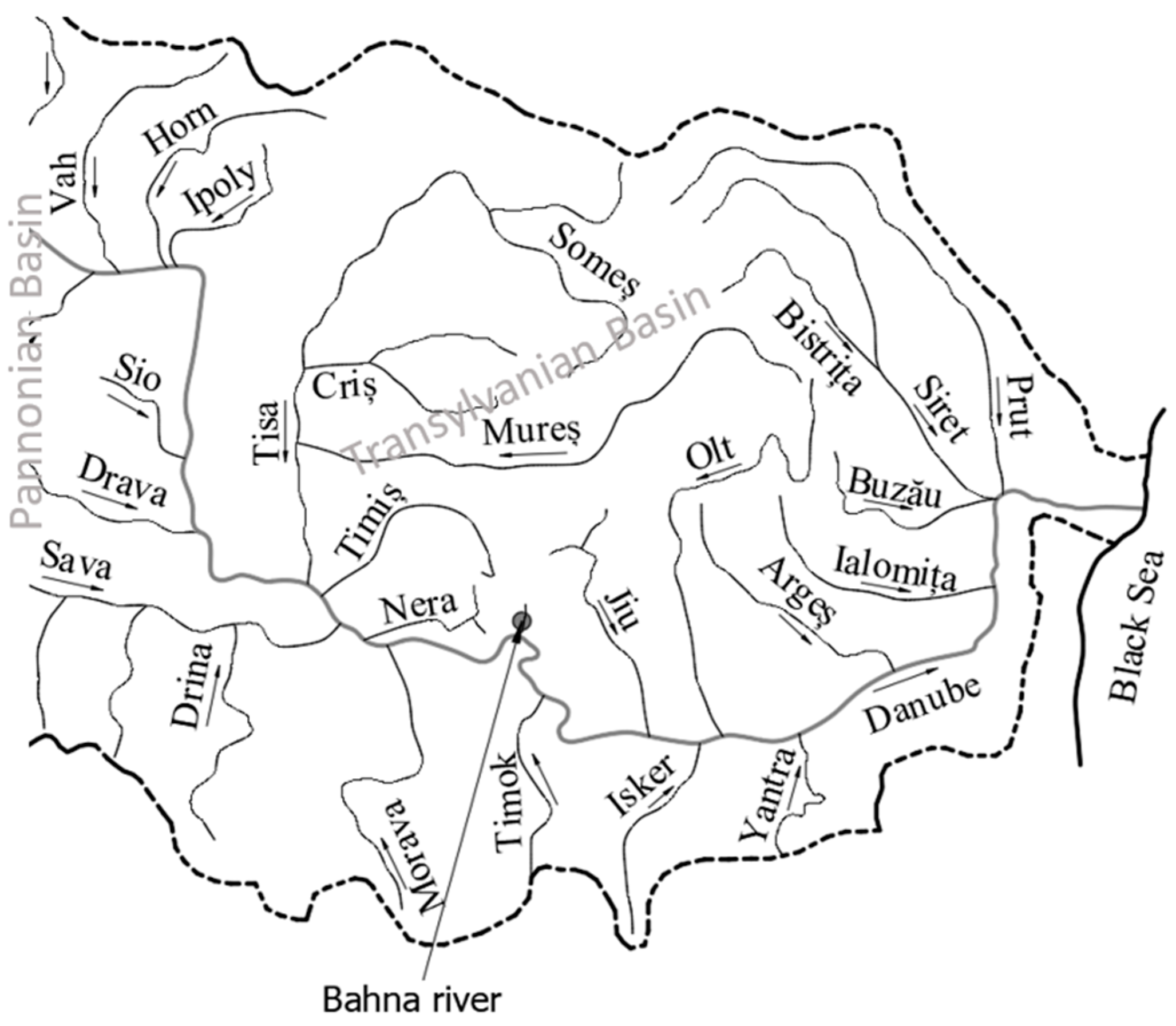
The Bahna River is part of the Danube River basin, being a left tributary. It is located in the south-west of Romania, as shown in Figure 2. The Cadastral code of the Bahna River is XIV.1.21.0.0.0.0 [47]. From a morpho-hydrographic point of view, the Bahna River is part of a sector of the Carpathian Gorges, this sector being the first of five sectors that divide the Danube River on the Romania territory [48]. The river is located on the border of the Pannonian Basin and the Transylvanian Basin.

As for its main morphometric characteristics, the Bahna River has a length of 35 km, an average stream slope of 28‰, a sinuosity coefficient of 1.45, an average altitude of 559 m and a watershed area of 137 km² [47]. The river is characterized by a very high torrentiality, with maximum recorded flows between 0.55 and 93.5m³/s.

The maximum annual series of maximum flows has a length of 30 records, from 1992 to 2021, as presented in Table 1.

The expected value, standard deviation, skewness and kurtosis have the values of 13.3 m³/s, 20.2 m³/s, 3.11 and 13.03. Table 2 shows the first four linear moments, the L–skewness and the L–kurtosis of the sample, for both methods.

For L-moments, the

L_{1}, L_{2}, L_{3}

and

L_{4}

are 13.3 m³/s, 8.07 m³/s, 4.91 m³/s and 3.52 m³/s. The values for the L-coefficient of variation (

τ_{2}

),L-skewness (

τ_{3}

) and L-kurtosis (

τ_{4}

) are 0.6083, 0.6079 and 0.4356. For the first order LH-moments, the first four linear moments are 21.3 m³/s, 9.73 m³/s, 5.62 m³/s and 3.68 m³/s. The values for the LH-coefficient of variation (

τ_{H 2}

),LH-skewness (

τ_{H 3}

) and LH-kurtosis (

τ_{H 4}

) are 0.4561, 0.5769 and 0.3781. For the second order LH-moments, the first four linear moments are 27.8 m³/s, 11.2 m³/s, 6.11 m³/s and 3.85 m³/s. The values for

τ_{H 2}, τ_{H 3}

and

τ_{H 4}

are 0.4009, 0.548 and 0.3451.

4. Results and Discussions

The analyzed models were applied for forecasting the rare events, with certain exceedance probabilities, for the Bahna River, Romania, as a case study.

4.1. The Inverse Function Results

Table 3 shows the quantiles results, characteristic of the range of the small exceedance probabilities (0.01–5%) necessary for the design of the hydrotechnical retention construction (dams), as well as the values corresponding to the exceedance probabilities of 40% and 80%, respectively, necessary for the delimitation of the bankfull channel.

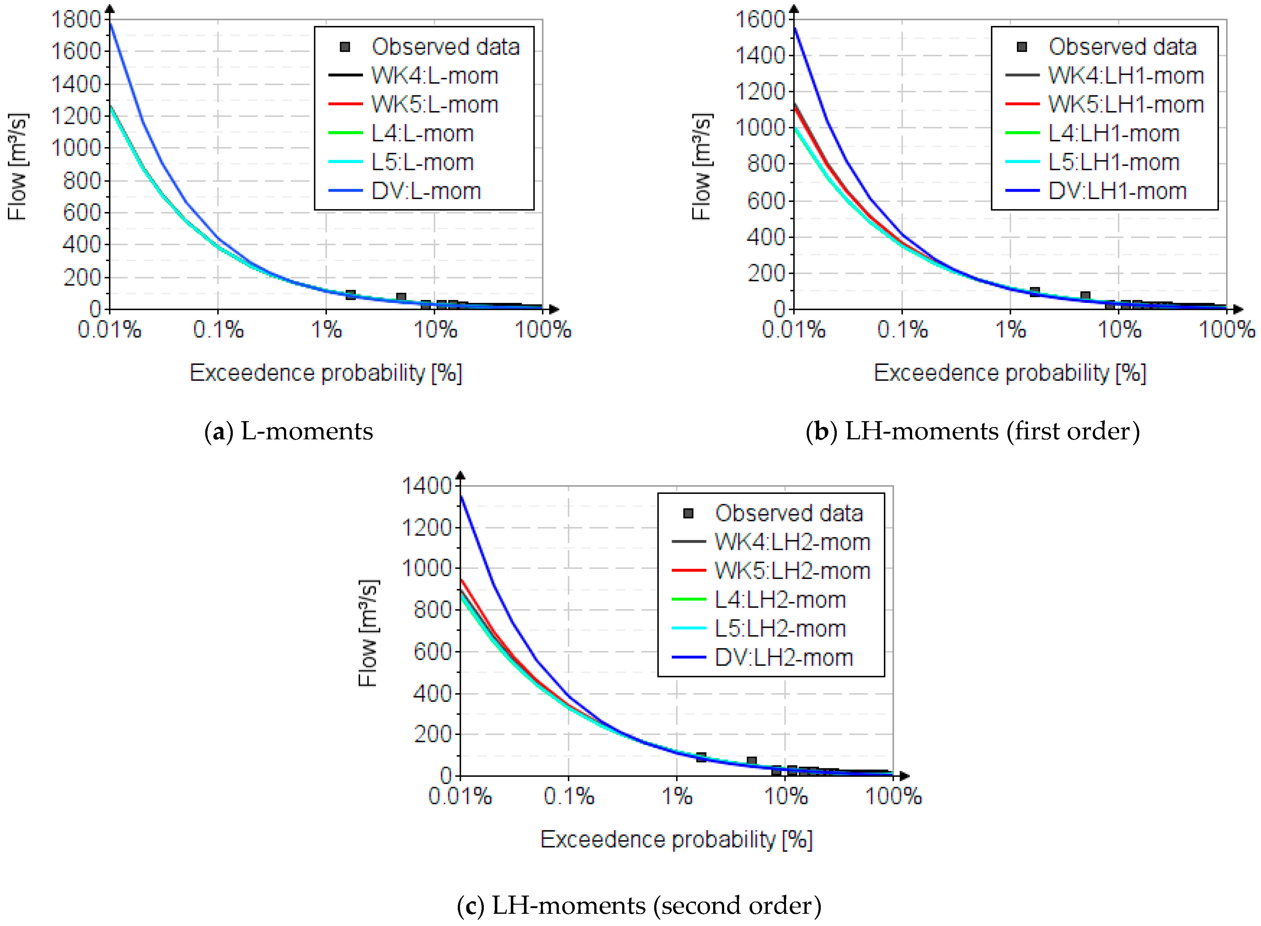
For the L-moments, the resulting quantile values, in the area of low exceedance probability, especially for the probability of 0.01%, varies between 1770 m³/s for the Davis distribution and 1250 m³/s for the Lambda distribution. The Wakeby distributions generate values close to those of the Lambda distributions, with values between 1256 m³/s and 1259 m³/s. For the first order LH-moments, the values are 1552 m³/s for the Davis distribution, 999 m³/s for the L4 distribution, 1006 m³/s for the L5 distribution, 1135 m³/s for the WK4 distribution and 1111 m³/s for the WK5 distribution. The second order LH-moments generate lower values of the maximum flows, namely 1349 m³/s for the Davis distribution, 862 m³/s for the L4 distribution, 869 m³/s for the L5 distribution, 1020 m³/s for the WK4 distribution and 949 m³/s for the WK5 distribution.

Figure 3 shows the quantile graphical results for the Bahna River. The proper empirical probability for L-moments is the Hazen formula [48,49], also chosen for the graphic representation of the data recorded for the Bahna River. The results of interest are those corresponding to probabilities between 0.01% and 1%, these being values of interest in the design of hydrotechnical constructions.

4.2. The Results Regarding the Parameter Estimation

Considering that to calibrate the parameters for WK5 and WK4, it is necessary to solve some systems of nonlinear equations, it is recommended to use the approximate relations presented by [29,30] as starting values (initial values), thus facilitating the ease of calculation. Table A1 from Appendix C presents the parameter values for the two methods and for the five analyzed distributions.

As observed in other materials [4,29,30], the Wakeby and Lambda distributions can become, in certain special cases, the generalized Pareto type II distribution and the three–parameter Tukey distribution, respectively, which has the following expressions of the inverse functions:

-: generalized Pareto Type II distribution [2,29,33]:

x (p) = γ + \frac{α}{β} \cdot (1 - p^{β})

(51)

-: Tukey distribution [30]:

x (p) = γ + α \cdot p^{β}

(52)

The same transformation occurs in the case of the frequency analysis on the Bahna River, where in the case of the WK4 distribution, the term

\frac{α}{β} \cdot (1 - p^{β})

has a constant value equal to 1.2433 for the L-moments, 0.766 in the case of first order LH-moments, respectively, and −0.133 in the case of the second order LH-moments. In the case of the WK5 distribution, the term

\frac{α}{β} \cdot (1 - p^{β})

has a constant value equal to −2.84 for the L-moments, −15.35 in the case of first order LH-moments, respectively, and −11.56 in the case of second order LH-moments.

For the L5 distribution, the term

λ \cdot {(1 - p)}^{δ}

has a constant value equal to 40.3 for the L-moments method, 44.5 in the case of first order LH-moments, respectively, and 49.3 in the case of second order LH-moments. For the L4 distribution, the term

λ \cdot {(1 - p)}^{δ}

has a constant value equal to 10.5 for the L-moments method, 18.5 in the case of first order LH-moments, respectively, and 26.6 in the case of second order LH-moments.

4.3. Selecting the Best Fit Model

The distributions performance and the choice of the best model is based on the natural (theoretical values) L-skewness and L-kurtosis values of the distributions, by comparing them with those of the observed data and choosing the one that has values close to those of the data set.

Additionally, two performance indicators that are usually applied in these types of analysis are presented: relative absolute error (RAE) and relative mean error (RME).

Table 4, Table 5 and Table 6 present the performance indicators’ values for the analyzed methods.

For the Bahna River, using the L-moments and the first and second order LH-moments, any of the Wakeby and Lambda distributions can be applied, considering that the quantile results are very close, and these distributions calibrate all linear moments accordingly. The theoretical values (

τ_{3}, τ_{4}, τ_{H 3}

and

τ_{H 4}

) of the distributions, namely 0.6079 and 0.4356 for L-moments, 0.5769 and 0.3781 for first order LH-moments, respectively, and 0.548 and 0.3451 for second order LH-moments, are the same as those of the analyzed data set.

Regarding the RAE and RME [50] results, they are indicative in nature as they highlight the performance of the distributions only in the area of the probability of exceeding the observed data, losing their relevance outside this domain.

4.4. Uncertainties

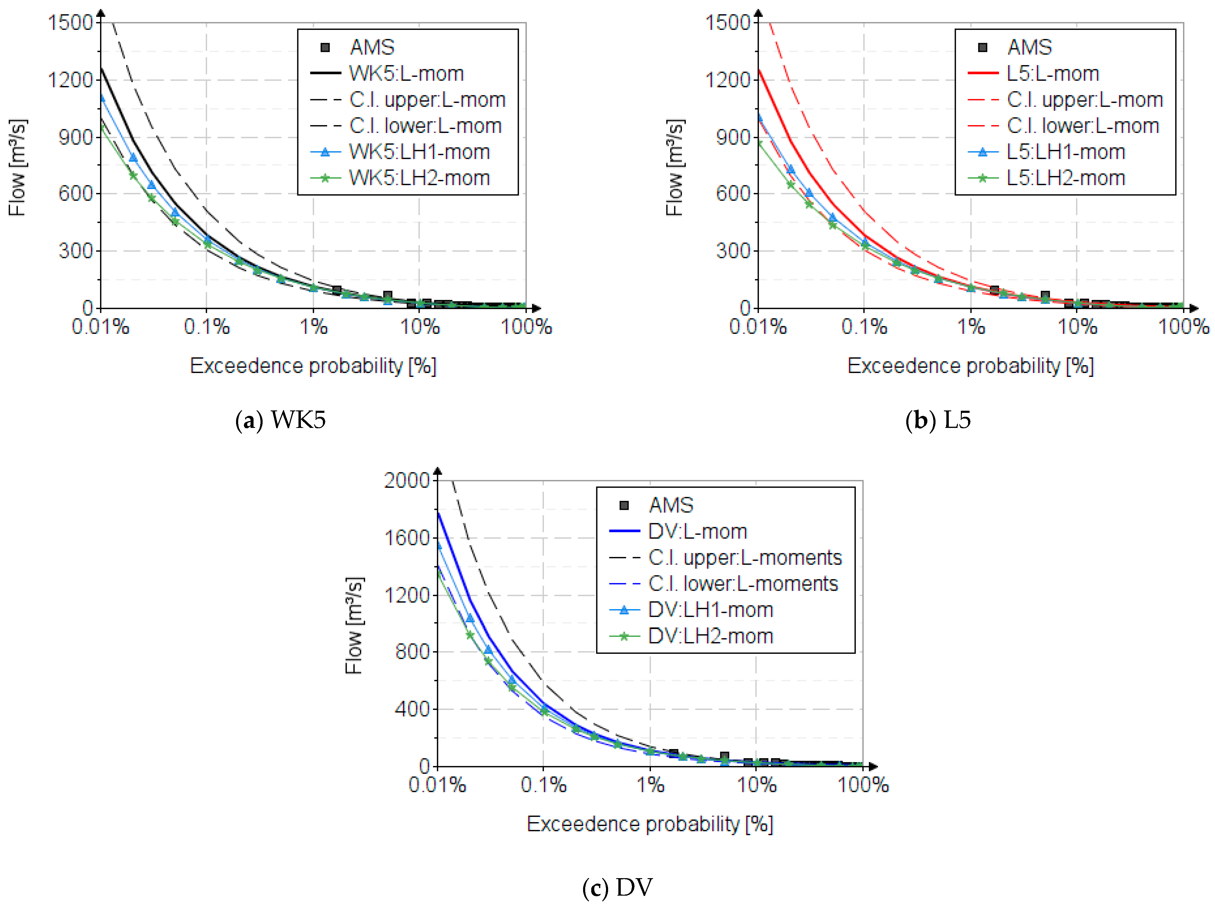
All the quantiles that exceed the probabilities of the recorded values are characterized by a high degree of uncertainty [51,52], due to the relatively short length of the observed data, a general disadvantage encountered in hydrometry in Romania. In the case of the Davis distribution, the high level of uncertainty is also due to the fact that, being a three–parameter distribution, it does not properly calibrate the fourth order linear moment. As could be seen in previous materials [2,3,8,9,29,32], although the L-moments method is more stable and robust than other methods, in terms of the variation of statistical indicators depending on the length of the observed data, this method also requires a minor correction, and the advantage of the stability of the indicators can be lost due to the non–linear functions for obtaining the parameters, an aspect highlighted very well by Gaume [53].

In general, the relative errors generated by the variability of the length of the recorded data are determined both in the estimation of the statistical indicators specific to the method used, as well as for the values of the parameters and quantiles, thus resulting in three levels of uncertainty. Thus, it is necessary to determine the confidence interval for each distribution and the method of estimating the parameters.

In Figure 4, the confidence interval for the KW5, KW4 and DV distributions is presented, for both methods, using Chow’s relation [54,55,56,57] for a 95% confidence level, based on a Gaussian assumption.

5. Conclusions

The article highlights the main elements necessary to apply the Wakeby, Lambda and Davis distributions in FFA using L-moments and the first and second LH-moments.

The estimation relations, as well as the frequency factors necessary to determine the confidence interval, are presented.

As a case study, the stages and rare events results on the Bahna river, Romania, using the first two levels of linear moments for parameter estimation are presented. The results are presented in comparison with the L-moments method, this being the proposed method to be implemented as the future norm in Romania.

The LH-moments method is a method usually applied in FFA without censored samples, which achieves the “separation effect” by giving less importance to the lower recorded values, which are, not in every case, floods.

Among the analyzed distributions, the Wakeby distribution is a general distribution applied in FFA. It was introduced by Hougthon precisely to fulfill this “separation effect”, and it is a distribution that has, as a special case, the generalized Pareto distribution of type II.

The purpose of this article is to present the main elements of the family of distributions, defined only by the quantile function, in FFA, using the L-moments method and the first and second level LH-moments method.

Regarding the results obtained for the Bahna river, the best model has the distributions WK5, WK4, L5 and L4, and the natural values of the statistical indicators L-skewness and L-kurtosis, best modeling the corresponding values of the observed data. This is due to the fact that the distributions are at least 4, thus succeeding in calibrating the L-moments tours. For the Davis distribution, it fails to properly calibrate the fourth order linear moment because it is a three-parameter distribution. This, like all distributions with a maximum of 3 parameters, is recommended to be applied only for data series with values of statistical indicators close to the natural ones of the distribution. This is also the main selection criterion of the best fit distribution, specific to these methods.

This result does not exclude other distributions, in a broader and more complex analysis, in determining the maximum flow on this river.

The research is part of a larger research within the Faculty of Hydrotechnics, in which all families of distributions used in FFA were analyzed, including the results presented in previous materials. The final goal of the research is the identification of the distribution probabilities and methods of estimating their parameters with applicability in FFA to the hydrological specifics of Romania.

The results will be concretized in open-source computer applications, which will be included in the new regulations.

Author Contributions

Conceptualization, C.G.A., S.C.S. and C.I.; methodology, C.G.A., S.C.S. and C.I.; software, C.G.A., S.C.S. and C.I.; vali-dation, C.G.A., S.C.S. and C.I.; formal analysis, C.G.A., S.C.S. and C.I.; investigation, C.G.A., S.C.S. and C.I.; resources, C.G.A., S.C.S. and C.I.; data curation, C.G.A., S.C.S. and C.I.; writing—original draft preparation C.G.A. and C.I.; writing—review and editing, C.G.A., S.C.S. and C.I.; visualization, C.G.A., S.C.S. and C.I.; supervision, C.I. and C.G.A.; project administration, C.G.A., S.C.S. and C.I.; funding acquisition, C.G.A., S.C.S. and C.I. All authors have read and agreed to the published version of the manuscript.

Funding

This research received no external funding.

Data Availability Statement

Not applicable.

Conflicts of Interest

The authors declare no conflict of interest.

Appendix A. The Frequency Factors

The frequency factor of the WK5 distribution and WK4 distribution is the same because the position parameter is reduced. The same is for the L5 and L4 distributions.

The quantile function (inverse function) can be expressed using the following relations:

-

for L-moments:

x (p) = L_{1} + L_{2} \cdot K_{p} (p)

-

for LH-moments:

x (p) = L_{H 1} + L_{H 2} \cdot K_{p} (p)

The frequency factors are:

Wakeby distribution:

-: L-moments:

$K_{p} (p) = \frac{\frac{α}{β} \cdot (1 - p^{β}) - \frac{γ}{δ} \cdot (1 - p^{- δ}) - \frac{α}{β + 1} - \frac{γ}{1 - δ}}{\frac{α}{(β + 1) \cdot (β + 2)} + \frac{γ}{(2 - δ) \cdot (1 - δ)}}$
-: LH-moments (first order):

$K_{p} (p) = \frac{\frac{α}{β} \cdot (1 - p^{β}) - \frac{γ}{δ} \cdot (1 - p^{- δ}) - \frac{α \cdot β + 3 \cdot α}{(β + 1) \cdot (β + 2)} - \frac{γ \cdot (δ - 3)}{(δ - 2) \cdot (δ - 1)}}{\frac{3 \cdot α}{(β + 1) \cdot (β + 2) \cdot (β + 3)} - \frac{3 \cdot γ}{(δ - 3) \cdot (δ - 2) \cdot (δ - 1)}}$
-: LH-moments (second order):

$K_{p} (p) = \frac{\frac{α}{β} \cdot (1 - p^{β}) - \frac{γ}{δ} \cdot (1 - p^{- δ}) - \frac{α \cdot β^{2} + 6 \cdot α \cdot β + 11 \cdot α}{(β + 1) \cdot (β + 2) \cdot (β + 3)} + \frac{γ \cdot (δ^{2} - 6 \cdot δ + 11)}{(δ - 3) \cdot (δ - 2) \cdot (δ - 1)}}{\frac{12 \cdot α}{(β + 1) \cdot (β + 2) \cdot (β + 3) \cdot (β + 4)} + \frac{12 \cdot γ}{(δ - 4) \cdot (δ - 3) \cdot (δ - 2) \cdot (δ - 1)}}$

Lambda distribution:

-: L-moments:

$\frac{\frac{p^{β} \cdot (α \cdot β + α) - λ \cdot (β + 1) \cdot {(1 - p)}^{δ} - α}{β + 1} + \frac{λ}{δ + 1}}{- \frac{α \cdot β}{(β + 1) \cdot (β + 2)} - \frac{λ \cdot δ}{(δ + 1) \cdot (δ + 2)}}$
-: LH-moments (first order):

$K_{p} (p) = \frac{\frac{2 \cdot α}{(β + 1) \cdot (β + 2)} + λ \cdot {(1 - p)}^{δ} - α \cdot p^{β} + \frac{2 \cdot λ}{δ + 2}}{\frac{3 \cdot α \cdot β}{(β + 1) \cdot (β + 2) \cdot (β + 3)} + \frac{3 \cdot λ \cdot δ}{2 \cdot (δ + 2) \cdot (δ + 3)}}$
-: LH-moments (second order):

$K_{p} (p) = \frac{\frac{6 \cdot α}{(β + 1) \cdot (β + 2) \cdot (β + 3)} + λ \cdot {(1 - p)}^{δ} - α \cdot p^{β} + \frac{3 \cdot λ}{δ + 3}}{\frac{12 \cdot α \cdot β}{(β + 1) \cdot (β + 2) \cdot (β + 3) \cdot (β + 4)} + \frac{2 \cdot λ \cdot δ}{(δ + 3) \cdot (δ + 4)}}$

Davis distribution:

-: L-moments:

$\frac{\frac{p^{α}}{{(1 - p)}^{λ}} - \frac{α \cdot Γ (α) \cdot (1 - λ)}{Γ (α + 2 - λ)}}{\frac{α \cdot π \cdot Γ (α) \cdot (λ + α)}{Γ (α - λ) \cdot (λ - α - 2) \cdot (λ - α - 1) \cdot (λ - α) \cdot Γ (λ) \cdot \sin (λ \cdot π)}}$
-: LH-moments (first order):

$K_{p} (p) = \frac{\frac{p^{α}}{{(1 - p)}^{λ}} - \frac{2 \cdot Γ (α + 1) \cdot (2 - λ)}{Γ (α + 3 - λ)}}{\frac{3 \cdot α \cdot π \cdot Γ (α) \cdot (λ + 2 \cdot α) \cdot (λ - 1)}{Γ (α - λ) \cdot 2 \cdot (λ - α - 3) \cdot (λ - α - 2) \cdot (λ - α - 1) \cdot (λ - α) \cdot Γ (λ) \cdot \sin (λ \cdot π)}}$
-: LH-moments (second order):

$K_{p} (p) = \frac{\frac{p^{α}}{{(1 - p)}^{λ}} - \frac{3 \cdot Γ (α + 1) \cdot (3 - λ)}{Γ (α - λ + 4)}}{\frac{2 \cdot γ \cdot α \cdot π \cdot Γ (α) \cdot (λ + 3 \cdot α) \cdot (λ - 2) \cdot (λ - 1)}{Γ (α - λ) \cdot (λ - α - 4) \cdot (λ - α - 3) \cdot (λ - α - 2) \cdot (λ - α - 1) \cdot (λ - α) \cdot Γ (λ) \cdot \sin (λ \cdot π)}}$

Appendix B. The Relationship between L-Moments and LH-Moments

Relations for LH-moments [8]:

L_{1}^{η} = E [X_{(η + 1) : (η + 1)}]

L_{2}^{η} = \frac{1}{2} \cdot E [X_{(η + 2) : (η + 2)} - X_{(η + 1) : (η + 2)}]

L_{3}^{η} = \frac{1}{3} \cdot E [X_{(η + 3) : (η + 3)} - 2 \cdot X_{(η + 2) : (η + 3)} + X_{(η + 1) : (η + 3)}]

L_{4}^{η} = \frac{1}{4} \cdot E [X_{(η + 4) : (η + 4)} - 3 \cdot X_{(η + 3) : (η + 4)} + 3 \cdot X_{(η + 2) : (η + 4)} - X_{(η + 1) : (η + 4)}]

unde

η = 0, 1, 2, 3, \dots

For

η = 0

, the method is identical to the L-moments method.

Based on these LH-moments, the reports

τ_{H 2}, τ_{H 3}, τ_{H 4}

are defined as follows:

τ_{H 2} = \frac{L_{2}^{η}}{L_{1}^{η}}

—represents LH-CV (coefficient of LH-variation)

τ_{H 3} = \frac{L_{3}^{η}}{L_{2}^{η}}

—represents LH-Cs (LH-skewness)

τ_{H 4} = \frac{L_{4}^{η}}{L_{2}^{η}}

—represents LH-Ck (LH-kurtosis)

The relations between the high-order linear moments and the normalized weighted moments are the following [8]:

L_{1}^{η} = B_{η}

L_{2}^{η} = \frac{(η + 2)}{2} \cdot (B_{η + 1} - B_{η})

L_{3}^{η} = \frac{(η + 3)}{6} \cdot ((η + 4) \cdot B_{η + 2} - 2 \cdot (η + 3) \cdot B_{η + 1} + (η + 2) \cdot B_{η})

L_{4}^{η} = \frac{(η + 4)}{24} \cdot (\begin{array}{l} (η + 6) \cdot (η + 5) \cdot B_{η + 3} - 3 \cdot (η + 5) \cdot (η + 4) \cdot B_{η + 2} + \\ 3 \cdot (η + 4) \cdot (η + 3) \cdot B_{η + 1} - (η + 3) \cdot (η + 2) \cdot B_{η} \end{array})

where

B_{η} = (η + 1) \cdot b_{η}

and

b_{η}

represent the natural estimators expressed by the L-moments method. For

η = 0

, the method become the L-moments method.

Appendix C. Estimated Parameter Values

Table A1 shows the values of the estimated parameters with the two analyzed estimation methods.

This is an important aspect regarding the transparency of the analysis and the possibility that the results can be reproduced

Table A1. Parameters estimated for the two methods.

Parameters	Distribution
Parameters	WK5	WK4	L5	L4	DV
L-moments
$α$	−1053	99,283,255	11.7	11.7	−0.608
$β$	369.6	79,851,895	−0.508	−0.508	–
$γ$	5.89	5.89	29.8	–	6.56
$δ$	0.51	–	0.001	0.004	–
$λ$	–	0.5104	40.3	10.5	−0.61
$ξ$	4.07	–	–	–	–
LH-moments (first order)
$α$	−275	124,323,093	16.5	16.7	−0.579
$β$	17.9	162,271,924	−0.4479	−0.446	–
$γ$	6.56	6.38	26.5	–	7.48
$δ$	0.4785	0.4852	0.0399	0.1075	–
$λ$	–	–	44.6	18.5	–0.8
$ξ$	15.7	–	–	–	–
LH-moments (second order)
$α$	−58.2	−1038	21.6	22	−0.548
$β$	5.04	7787	−0.4046	−0.4017	–
$γ$	7.67	7.04	23.4	–	8.68
$δ$	0.4348	–	0.0834	0.1724	–
$λ$	–	0.4569	49.3	26.7	−1.084
$ξ$	10.2	–	–	–	–

References

Houghton, C. Birth of a Parent: The Wakeby Distribution for Modeling Flood Flows; Working Paper no. MIT–EL77–033WP; Water Resources Research: Tucson, AZ, USA, 1978; Volume 14. [Google Scholar]
Anghel, C.G.; Ilinca, C. Evaluation of Various Generalized Pareto Probability Distributions for Flood Frequency Analysis. Water 2023, 15, 1557. [Google Scholar] [CrossRef]
Ilinca, C.; Anghel, C.G. Flood Frequency Analysis Using the Gamma Family Probability Distributions. Water 2023, 15, 1389. [Google Scholar] [CrossRef]
Ilinca, C.; Anghel, C.G. Flood–Frequency Analysis for Dams in Romania. Water 2022, 14, 2884. [Google Scholar] [CrossRef]
Anghel, C.G.; Ilinca, C. Parameter Estimation for Some Probability Distributions Used in Hydrology. Appl. Sci. 2022, 12, 12588. [Google Scholar] [CrossRef]
Anghel, C.G.; Ilinca, C. Hydrological Drought Frequency Analysis in Water Management Using Univariate Distributions. Appl. Sci. 2023, 13, 3055. [Google Scholar] [CrossRef]
Ilinca, C.; Anghel, C.G. Frequency Analysis of Extreme Events Using the Univariate Beta Family Probability Distributions. Appl. Sci. 2023, 13, 4640. [Google Scholar] [CrossRef]
Wang, Q.J. LH moments for statistical analysis of extreme events. Water Resour. Res. 1997, 33, 2841–2848. [Google Scholar] [CrossRef]
Md Sharwar, M.; Park, B.-J.; Jeong, B.-Y.; Park, J.-S. LH-Moments of Some Distributions Useful in Hydrology. Commun. Stat. Appl. Methods 2009, 16, 647–658. [Google Scholar]
Hewa, G.A.; Wang, Q.J.; McMahon, T.A.; Nathan, R.J.; Peel, M.C. Generalized extreme value distribution fitted by LH moments for low–flow frequency analysis. Water Resour. Res. 2007, 43, W06301. [Google Scholar] [CrossRef] [Green Version]
Fawad, M.; Cassalho, F.; Ren, J.; Chen, L.; Yan, T. State-of-the-Art Statistical Approaches for Estimating Flood Events. Entropy 2022, 24, 898. [Google Scholar] [CrossRef]
Lee, S.H.; Maeng, S.J. Comparison and analysis of design floods by the change in the order of LH-moment methods. Irrig. Drain. 2003, 52, 231−245. [Google Scholar] [CrossRef]
Meshgi, A.; Davar, K. Comprehensive evaluation of regional flood frequency analysis by L- and LH-moments. II. Development of LH-Moments parameters for the generalized Pareto and generalized logistic distributions. Stoch. Environ. Res. Risk Assess. 2009, 23, 137−152. [Google Scholar] [CrossRef]
Meshgi, A.; Khalili, D. Comprehensive evaluation of regional flood frequency analysis by L- and LH-moments. I. A revisit to regional homogeneity. Stoch. Environ. Res. Risk Assess. 2009, 23, 119–135. [Google Scholar] [CrossRef]
Bhuyan, A.; Borah, M.; Kumar, R. Regional Flood Frequency Analysis of North–Bank of the River Brahmaputra by Using LH-Moments. Water Resour. Manag. 2010, 24, 1779–1790. [Google Scholar] [CrossRef]
Gheidari, M.H.N. Comparisons of the L- and LH-Moments in the selection of the best distribution for regional flood frequency analysis in Lake Urmia Basin. Civ. Eng. Environ. Syst. 2013, 30, 72–84. [Google Scholar] [CrossRef]
Abida, H.; Ellouze, M. Probability distribution of flood flows in Tunisia. Hydrol. Earth Syst. Sci. 2008, 12, 703–714. [Google Scholar] [CrossRef] [Green Version]
Aydogan, D.; Kankal, M.; Onsoy, H. Regional flood frequency analysis for Coruh Basin of Turkey with L-moments approach. J. Flood Risk Manag. 2016, 9, 69–86. [Google Scholar] [CrossRef]
De Luca, D.L.; Napolitano, F. A user–friendly software for modelling extreme values: EXTRASTAR (extremes abacus for statistical regionalization. Environ. Model. Softw. 2023, 161, 105622. [Google Scholar] [CrossRef]
Haddad, K.; Rahman, A. Regional flood frequency analysis in eastern Australia: Bayesian GLS regression-based methods within fixed region and ROI framework—Quantile regression vs. parameters regression technique. J. Hydrol. 2012, 430–431, 142–161. [Google Scholar] [CrossRef]
Hussain, T.; Pasha, G. Regional flood frequency analysis of the seven sites of Punjab, Pakistan, using L-moments. Water Resour. Manag. 2009, 23, 1917–1933. [Google Scholar] [CrossRef]
Laio, F.; Ganora, D.; Claps, P.; Galeati, G. Spatially smooth regional estimation of the flood frequency curve (with uncertainty). J. Hydrol. 2011, 408, 67–77. [Google Scholar] [CrossRef]
Noto, V.L.; La Loggia, G. Use of L-moments approach for regional flood frequency analysis in Sicily, Italy. Water Resour. Manag. 2009, 23, 2207–2229. [Google Scholar] [CrossRef]
Saf, B. Regional flood frequency analysis using L-moments for the West Mediterranean region of Turkey. Water Resour. Manag. 2009, 23, 531–551. [Google Scholar] [CrossRef]
Seckin, N.; Haktanir, T.; Yurtal, R. Flood frequency analysis of Turkey using L-moments method. Hydrol. Process. 2011, 25, 3499–3505. [Google Scholar] [CrossRef]
Deka, S.; Borah, M.; Kakaty, S.C. Statistical analysis of annual maximum rainfall in North–East India: An application of LH-moments. Theor. Appl. Climatol. 2011, 104, 111–122. [Google Scholar] [CrossRef]
Zakaria, Z.; Suleiman, J.; Mohamad, M. Rainfall frequency analysis using LH-Moments approach: A case of Kemaman Station, Malaysia. Int. J. Eng. Technol. 2018, 7, 107−110. [Google Scholar] [CrossRef] [Green Version]
Bora, D.; Borah, M.; Bhuyan, A. Regional analysis of maximum rainfall using L-moment and LH-moment: A comparative case study for the northeast India. Mausam 2017, 68, 451−462. [Google Scholar] [CrossRef]
Rao, A.R.; Hamed, K.H. Flood Frequency Analysis; CRC Press LLC: Boca Raton, FL, USA, 2000. [Google Scholar]
Greenwood, J.A.; Landwehr, J.M.; Matalas, N.C.; Wallis, J.R. Probability Weighted Moments: Definition and Relation to Parameters of Several Distributions Expressable in Inverse Form. Water Resour. Res. 1979, 15, 1049–1054. [Google Scholar] [CrossRef] [Green Version]
Hosking, J.R.M. L-moments: Analysis and Estimation of Distributions using Linear, Combinations of Order Statistics. J. R. Statist. Soc. 1990, 52, 105–124. [Google Scholar] [CrossRef]
Hosking, J.R.M.; Wallis, J.R. Regional Frequency Analysis: An Approach Based on L-Moments; Cambridge University Press: Cambridge, UK, 1997. [Google Scholar] [CrossRef]
Singh, V.P. Entropy–Based Parameter Estimation in Hydrology; Springer Science + Business Media: Dordrecht, The Netherlands, 1998; ISBN 978-90-481-5089-2/978-94-017-1431-0. [Google Scholar]
Khan, Z.; Rahman, A.; Karim, F. An Assessment of Uncertainties in Flood Frequency Estimation Using Bootstrapping and Monte Carlo Simulation. Hydrology 2023, 10, 18. [Google Scholar] [CrossRef]
Bobée, B.; Cavadias, G.; Ashkar, F.; Bernier, J.; Rasmussen, P. Towards a Systematic Approach to Comparing Distributions Used in Flood Frequency Analysis. J. Hydrol. 1993, 142, 121–136. [Google Scholar] [CrossRef]
Leščešen, I.; Dolinaj, D. Regional Flood Frequency Analysis of the Pannonian Basin. Water 2019, 11, 193. [Google Scholar] [CrossRef] [Green Version]
Sun, P.; Zhang, Q.; Yao, R.; Singh, V.P.; Song, C. Low Flow Regimes of the Tarim River Basin, China: Probabilistic Behavior, Causes and Implications. Water 2018, 10, 470. [Google Scholar] [CrossRef] [Green Version]
Öztekin, T. Wakeby distribution for representing annual extreme and partial duration rainfall series. Meteorol. Appl. 2007, 14, 381–387. [Google Scholar]
Chang, C.-H.; Rahmad, R.; Wu, S.-J.; Hsu, C.-T. Spatial Frequency Analysis by Adopting Regional Analysis with Radar Rainfall in Taiwan. Water 2022, 14, 2710. [Google Scholar] [CrossRef]
Wei, T.; Song, S. Confidence Interval Estimation for Precipitation Quantiles Based on Principle of Maximum Entropy. Entropy 2019, 21, 315. [Google Scholar] [CrossRef]
Busababodhin, P.; Seo, Y.A.; Park, J.S.; Kumphon, B.O. LH-moment estimation of Wakeby distribution with hydrological applications. Stoch. Environ. Res. Risk Assess. 2016, 30, 1757–1767. [Google Scholar] [CrossRef]
Busababodhin, P.; Monchaya, C.; Phoophiwfa, T.; Park, J.-S.; Manoon, D.-O.; Pannarat, G. LH-Moments of the Wakeby Distribution applied to Extreme Rainfall in Thailand. Malays. J. Fundam. Appl. Sci. 2021, 17, 166–180. [Google Scholar] [CrossRef]
Zalina, M.D.; Desa, M.N.M.; Nguyen, V.T.V.; Kassim, A.H.M. Selecting a probability distribution for extreme rainfall series in Malaysia. Water Sci. Technol. 2002, 45, 63–68. [Google Scholar] [CrossRef]
Machiwal, D.; Jha, M. Hydrologic Time Series Analysis: Theory and Practice; Springer: Berlin/Heidelberg, Germany, 2012. [Google Scholar] [CrossRef]
Ilona, J.; Bartók, B.; Dumitrescu, A.; Cheval, S.; Gandhi, A.; Tordai, Á.V.; Weidinger, T. Using Long–Term Historical Meteorological Data for Climate Change Analysis in the Carpathian Region. Atmosphere 2022, 13, 1751. [Google Scholar] [CrossRef]
Hankin, R.; Lee, A. A new family of non-negative distributions. Aust. New Zealand J. Stat. 2006, 48, 67–78. [Google Scholar] [CrossRef]
The Romanian Water Classification Atlas, Part I—Morpho-Hydrographic Data on the Surface Hydrographic Network; Ministry of the Environment: Bucharest, Romania, 1992.
Dau, Q.V.; Kangrang, A.; Kuntiyawichai, K. Probability–Based Rule Curves for Multi-Purpose Reservoir System in the Seine River Basin, France. Water 2023, 15, 1732. [Google Scholar] [CrossRef]
Van Campenhout, J.; Houbrechts, G.; Peeters, A.; Petit, F. Return Period of Characteristic Discharges from the Comparison between Partial Duration and Annual Series, Application to the Walloon Rivers (Belgium). Water 2020, 12, 792. [Google Scholar] [CrossRef] [Green Version]
Singh, V.P.; Singh, K. Parameter Estimation for Log-Pearson Type III Distribution by Pome. Hydraul. Eng. 1988, 114, 112–122. [Google Scholar] [CrossRef]
Kazemi, H.; Hashemi, H.; Maghsood, F.F.; Hosseini, S.H.; Sarukkalige, R.; Jamali, S.; Berndtsson, R. Climate vs. Human Impact: Quantitative and Qualitative Assessment of Streamflow Variation. Water 2021, 13, 2404. [Google Scholar] [CrossRef]
Semananda, N.P.K.; Hewa, G.A. Estimation of Low Flow Statistics for Sustainable Water Resources Management in South Australia. Hydrology 2022, 9, 152. [Google Scholar] [CrossRef]
Gaume, E. Flood frequency analysis: The Bayesian choice. WIREs Water 2018, 5, e1290. [Google Scholar] [CrossRef] [Green Version]
Chow, V.T.; Maidment, D.R.; Mays, L.W. Applied Hydrology; McGraw–Hill, Inc.: New York, NY, USA, 1988; ISBN 007-010810-2. [Google Scholar]
World Meteorological Organization. (WMO–No.718) 1989 Statistical Distributions for Flood Frequency Analysis; Operational Hydrology Report no. 33; WHO: Geneva, Switzerland, 1989. [Google Scholar]
Bulletin 17B Guidelines for Determining Flood Flow Frequency; Hydrology Subcommittee, Interagency Advisory Committee on Water Data, U.S. Departament of the Interior, U.S. Geological Survey, Office of Water Data Coordination: Reston, VA, USA, 1981.
Bulletin 17C Guidelines for Determining Flood Flow, Frequency; U.S. Department of the Interior, U.S. Geological Survey: Reston, VA, USA, 2017.

Figure 1. The stages of the methodological approach.

Figure 2. Location of the Bahna River in Romania.

Figure 3. The quantile results for the two parameter estimation methods.

Figure 4. The probability distributions curves with confidence intervals.

Table 1. The historical data.

Year		1992	1993	1994	1995	1996	1997	1998	1999	2000	2001	2002
Flow	[m³/s]	4.31	12.2	7.72	9.90	25.5	4.43	4.71	93.5	8.64	5.4	3.78
		2003	2004	2005	2006	2007	2008	2009	2010	2011	2012	2013
Flow	[m³/s]	1.85	3.75	19.6	70	2.25	1.35	22.9	7.65	3.66	8.80	13.2
		2014	2015	2016	2017	2018	2019	2020	2021
Flow	[m³/s]	27.4	13.2	3.64	0.554	4.95	4.04	2.71	6.47

Table 2. The sample linear moments.

Bahna River	Methods
	L-moments
	$L_{1}$	$L_{2}$	$L_{3}$	$L_{4}$	$τ_{2}$	$τ_{3}$	$τ_{4}$
	[m³/s]	[m³/s]	[m³/s]	[m³/s]	[−]	[−]	[−]
	13.3	8.07	4.91	3.52	0.6083	0.6079	0.4356
	LH-moments (first order)
	$L_{H 1}$	$L_{H 2}$	$L_{H 3}$	$L_{H 4}$	$τ_{H 2}$	$τ_{H 3}$	$τ_{H 4}$
	[m³/s]	[m³/s]	[m³/s]	[m³/s]	[−]	[−]	[−]
	21.3	9.73	5.62	3.68	0.4561	0.5769	0.3781
	LH-moments (second order)
	$L_{H 1}$	$L_{H 2}$	$L_{H 3}$	$L_{H 4}$	$τ_{H 2}$	$τ_{H 3}$	$τ_{H 4}$
	[m³/s]	[m³/s]	[m³/s]	[m³/s]	[−]	[−]	[−]
	27.8	11.2	6.11	3.85	0.4009	0.548	0.3451

Table 3. The inverse function results for the analyzed methods.

Distribution	Exceedance Probabilities [%]
	L-Moments
	0.01	0.1	0.5	1	2	3	5	40	80
WK5	1256	382	162	111	74.7	58.8	43	8.11	2.62
WK4	1259	382	162	111	74.7	58.8	43	8.12	2.63
L5	1250	381	162	111	74.8	58.9	43	8.10	2.63
L4	1250	381	162	111	74.8	58.9	43	8.10	2.63
DV	1770	437	163	107	70	54.2	39.3	8.38	2.81
	LH-Moments (First Order)
	0.01	0.1	0.5	1	2	3	5	40	80
WK5	1111	360	160	111	75.8	60.1	44.2	7.95	2.24
WK4	1135	363	160	110	75.4	59.7	43.9	8.13	2.27
L5	1006	347	159	112	77.3	61.5	45.2	7.69	2.92
L4	999	346	159	112	77.4	61.6	45.3	7.68	2.93
DV	1552	409	160	107	70.9	55.6	40.7	8.45	2.35
	LH-Moments (Second Order)
	0.01	0.1	0.5	1	2	3	5	40	80
WK5	949	337	158	112	77.7	62	45.9	7.36	4.16
WK4	1020	346	158	111	74.5	60.9	45	7.88	1.52
L5	869	327	158	113	79.1	63.2	46.7	7.32	3.82
L4	862	326	158	113	79.2	63.3	46.8	7.31	3.81
DV	1349	382	157	107	72.4	57.3	42.4	8.24	1.71

Table 4. Distributions performance values for L-moments.

Distribution	Probability Distributions				Observed Data
	L-Moments				Observed Data
	RME	RAE	$τ_{3}$	$τ_{4}$	$τ_{3}$	$τ_{4}$
WK5	0.0527	0.1474	0.6079	0.4356	0.6079	0.4356
WK4	0.0534	0.1473
L5	0.0584	0.1535
L4	0.0584	0.1534
DV	0.0269	0.1154		0.4746

Table 5. Distributions performance values for first order LH-moments.

Distribution	Probability Distributions				Observed Data
	LH-Moments (First Order)				Observed Data
	RME	RAE	$τ_{H 3}$	$τ_{H 4}$	$τ_{H 3}$	$τ_{H 4}$
WK5	0.697	0.9847	0.5769	0.3781	0.5769	0.3781
WK4	0.0382	0.1537
L5	0.2912	0.4683
L4	0.2735	0.4471
DV	0.0415	0.171		0.4190

Table 6. Distributions performance values for second order LH-moments.

Distribution	Probability Distributions				Observed Data
	LH-Moments (Second Order)				Observed Data
	RME	RAE	$τ_{H 3}$	$τ_{H 4}$	$τ_{H 3}$	$τ_{H 4}$
WK5	0.5648	0.9541	0.5480	0.3451	0.5480	0.3451
WK4	0.0712	0.2732
L5	0.5904	0.905
L4	0.5266	0.8235
DV	0.0624	0.2391		0.3788

Disclaimer/Publisher’s Note: The statements, opinions and data contained in all publications are solely those of the individual author(s) and contributor(s) and not of MDPI and/or the editor(s). MDPI and/or the editor(s) disclaim responsibility for any injury to people or property resulting from any ideas, methods, instructions or products referred to in the content.

© 2023 by the authors. Licensee MDPI, Basel, Switzerland. This article is an open access article distributed under the terms and conditions of the Creative Commons Attribution (CC BY) license (https://creativecommons.org/licenses/by/4.0/).

Share and Cite

MDPI and ACS Style

Anghel, C.G.; Stanca, S.C.; Ilinca, C. Extreme Events Analysis Using LH-Moments Method and Quantile Function Family. Hydrology 2023, 10, 159. https://0-doi-org.brum.beds.ac.uk/10.3390/hydrology10080159

AMA Style

Anghel CG, Stanca SC, Ilinca C. Extreme Events Analysis Using LH-Moments Method and Quantile Function Family. Hydrology. 2023; 10(8):159. https://0-doi-org.brum.beds.ac.uk/10.3390/hydrology10080159

Chicago/Turabian Style

Anghel, Cristian Gabriel, Stefan Ciprian Stanca, and Cornel Ilinca. 2023. "Extreme Events Analysis Using LH-Moments Method and Quantile Function Family" Hydrology 10, no. 8: 159. https://0-doi-org.brum.beds.ac.uk/10.3390/hydrology10080159

Note that from the first issue of 2016, this journal uses article numbers instead of page numbers. See further details here.

Article Menu

Extreme Events Analysis Using LH-Moments Method and Quantile Function Family

Abstract

1. Introduction

2. Methods

2.1. Quantile Functions

2.2. The L- and LH-Moments Estimations Equations

2.2.1. The Five-Parameter Wakeby Distribution (WK5)

2.2.2. The Four-Parameter Wakeby Distribution (WK4)

2.2.3. The Five-Parameter Lambda Distribution (L5)

2.2.4. The Four-Parameter Lambda Distribution (L4)

2.2.5. Davis Distribution (DV)

3. Study Area and Main Data

4. Results and Discussions

4.1. The Inverse Function Results

4.2. The Results Regarding the Parameter Estimation

4.3. Selecting the Best Fit Model

4.4. Uncertainties

5. Conclusions

Author Contributions

Funding

Data Availability Statement

Conflicts of Interest

Appendix A. The Frequency Factors

Appendix B. The Relationship between L-Moments and LH-Moments

Appendix C. Estimated Parameter Values

References

Share and Cite

Article Metrics

Article Access Statistics

Further Information

Guidelines

MDPI Initiatives

Follow MDPI