Hydroclimatic Trends and Streamflow Response to Recent Climate Change: An Application of Discrete Wavelet Transform and Hydrological Modeling in the Passaic River Basin, New Jersey, USA

Abstract

The exigency of the current climate crisis demands a more comprehensive approach to addressing location-specific climate impacts. In the Passaic River Basin (PRB), two bodies of research—hydroclimatic trend detection and hydrological modeling—have been conducted with the aim of revealing the basin’s hydroclimate patterns as well as the hydrologic response to recent climate change. In a rather novel application of the wavelet transform tool, we sidelined the frequently used Mann–Kendal (MK) trend test, to identify the hidden monotonic trends in the inherently noisy hydroclimatic data. By this approach, the use of MK trend test directly on the raw data, whose results are almost always ambiguous and statistically insignificant in respect of precipitation data, for instance, no longer poses a challenge to the reliability of trend results. Our results showed that, whereas trends in temperature and precipitation are increasing in the PRB, streamflow trends are decreasing. Based on results from the hydrological modeling, streamflow is more sensitive to actual evapotranspiration (ET) than it is to precipitation. In periods spanning decades with sufficient water availability, energy governs actual evapotranspiration rates, rendering streamflow more sensitive to increases in precipitation. Conversely, during meteorologically stressed decades, water availability dictates actual evapotranspiration, consequently amplifying streamflow sensitivity to fluctuations in actual evapotranspiration. We found that the choice of baseline condition constitutes an important source of uncertainty in the sensitivities of streamflow to precipitation and evapotranspiration changes and should routinely be considered in any climate impact assessment.

1. Introduction

Global climate change is expected to accelerate the global hydrologic cycle, which will drive more intense floods and droughts leading to changes in streamflow and water resource availability. An alteration of the discharge regime of rivers [1,2] is usually the ultimate consequence. In the past decades, empirical evidence of warming-driven intensification of the hydrologic cycle has led to an increasing interest in the linkage of climatic variability or change to hydrological processes across space and time [3]. More often than not, the literature is either rich in the detection and analysis of hydroclimatic trends (e.g., [4,5,6]) or hydrological modeling studies (e.g., [7,8,9]), without considering both. For instance, ref. [10] underscored the importance of understanding climate variability and trends for the management and planning of water resources. Ref. [11] also investigated monthly and annual trends in temperature and precipitation and evaluated the significance of their variability for crop yields using multiple regression analysis. In another study, ref. [12] used the Soil and Water Assessment Tool (SWAT) model combined with land use and global climate models to examine how climate and land use/land cover work together to impact blue-green water in an arid basin. At a time when the global warming problem has evolved into a crisis [13,14], it is important that hydrological impact assessments be carried out from a holistic standpoint. Although the analysis and detection of trends can provide useful insights in terms of a general estimate of the direction and changes in magnitudes of hydrometeorological series, they lack the ability to predict unprecedented future conditions. Process-based models, although only capable of representing processes to the scope that they are quantitatively understood, can provide a robust framework for assessing hydrological response to climate change [15]. More so, because the direction and extent of changes in river flows are dependent on the relative balance between precipitation and the processes that govern evapotranspiration [15], the causes of discharge changes—which oftentimes seem controversial [16,17]—can effectively be examined from a hydrological modeling standpoint.

In studies that emphasize the detection and analysis of hydroclimatic trends (e.g., [16,17,18,19]), one statistical tool that has commonly been used is the nonparametric Mann–Kendall (MK) test and its modified forms. The MK trend test identifies changes in hydroclimatic series by simply fitting a monotonic (e.g., linear) trend at a certain time-period where a significant level is assigned by a statistical test. While the robustness of this test is not in doubt, its application to hydroclimatic time-series can be particularly challenging due to the nonmonotonic and nonuniform character of hydroclimatic variables. In many of these studies, trends in hydroclimatic variables, especially, precipitation, is found to be either not statistically significant or significant at a lower confidence level. For instance, in studying trends in precipitation, temperature, and streamflow at 13, 12, and 9 gauging stations, respectively, ref. [20] found that mean annual and seasonal precipitation trends were not statistically significant in all the gauging stations. In the entire Swat River Basin of Pakistan, ref. [21] observed that annual precipitation time-series did not show any statistically significant trends in all the subbasins examined. Ref. [6] also found that no statistically significant monotonic trend was detected for annual rainfall, although nonsignificant downward trends were dominant. Numerous studies with similar findings abound in the literature, and are usually in the application of Mann–Kendal tests to hydroclimatic time-series (e.g., [22,23,24,25,26]). Ref. [27] noted that, because the stochastic structure of time-series data has the tendency to assume trend-like features, analyzing trends in nonstationary time-series can cause a purely stochastic behavior to appear deterministic, leading to a likely erroneous interpretation of results. More so, because climatic phenomena and events (e.g., precipitation, hurricanes) are products of various complex atmospheric processes [28], noise is inevitably present, and this can affect the variability and trend in the data series. In hydroclimatic times series where nonmonotonicity is more the rule rather than the exception [29], identifying the hidden monotonic trend and assessing their statistical significance subsequently provide more reliable results than those derived from the direct trend analysis of the raw data [30].

Because the structure of hydroclimatic data is often hidden behind the noise, a precise mathematical operation that looks at the data through the noise and quantifies the structure present in the signal is needed. One such tool is the wavelet transform (WT). WT is a relatively recent development in the field of signal processing [31,32], and has, in recent times, emerged as an effective tool to analyze trends in hydroclimatic series especially in the atmospheric and hydrological science space [29,33,34,35,36,37,38]. It can be thought of as a ‘mathematical microscope’ with the ability to zoom in and out of the signal (or time series) to pull out the patterns. In its application, a signal or time-series data are decomposed into their low-frequency components and high-frequency components. The different decomposition levels, representing different periodic time scales, are subsequently analyzed for trends. The last decomposition level, which contains the lowest frequency component, usually represents the trend component of the time series. Thus, among the methods presently used in analyzing time-series data, the wavelet approach has the superior ability to handle the nonstationary characteristics of hydroclimatic time-series on multiple temporal resolutions [39], making it well suited for identifying trends over a long period of time.

In light of understanding and quantifying the hydrological impacts of climate variability/change, different approaches (i.e., conceptual methods, analytical, experimental, and hydrological modeling) have been used. Among these, process-based hydrological models provide a means to examine the physical mechanisms and processes that drive hydrological changes and variations. Their primary purpose is to partition precipitation into evapotranspiration and streamflow. They must, however, be thoroughly evaluated against field observations that sufficiently represent the region and timeframe of interest [40,41]. By applying a rigorously calibrated and validated physically based hydrological model, MIKE SHE, to the Rockaway catchment, a subbasin of the Passaic River Basin (PRB) in New Jersey, USA, we explored the mechanisms underpinning streamflow changes through the examination of MIKE SHE simulated water balance terms under various climate scenarios.

Thus, the novelty of this study lies in the application of advanced trend analysis tool with a physically based hydrological model that simulates both surface and subsurface flows in the land phase of the hydrological cycle. This combination will provide important clues on the key underlying variables behind the trend as well as insights into how hydroclimatic patterns may change into the future.

In the PRB and its surrounding areas, the lingering effects of a troubled history of improper environmental practices from the industrial boom continue to be experienced. According to [42], the Passaic River played a central role in the early development of New Jersey. In the late 18th century, the river served as navigable routes connected by a system of canals to the Delaware River. It was also an early source of hydroelectric power at the Great Falls in Paterson, making the region a focal point for industrial mills. Consequently, the lower Passaic experienced significant environmental contamination resulting from decades of industrial activity in the vicinity. By 1970, issues pertaining to flooding had already become apparent due to the presence of dams, and they continue to afflict the inhabitants of the basin at present. Furthermore, the intricate network of river systems amidst the heterogeneous biophysical landscape within the basin presents a complex array of conflicting interests and water-related challenges. In a region where increases in temperature [43,44] accompanied by evapotranspiration and snowpack depletion [15,45] are both observed and projected, the consequent impact on streamflow could be extensive. In light of these circumstances, our study undertakes a comprehensive hydrological impacts assessment in pursuit of establishing important foundations for the predictive understanding of the impacts of climate change on water resources in the PRB and its environs.

To this end, this research endeavor embraces a dual-fold objective: (1) Identifying shifts in hydrometeorological trends within the PRB spanning the period from 1979 to 2021; and (2) Investigating the responsiveness and sensitivities of hydrological systems to climatic phenomena in the Rockaway River basin, a subcatchment of the PRB. The analysis of hydroclimatic trends employs the discrete wavelet transform and Mann–Kendal test methodologies, while the evaluation of climate change implications in the PRB employs a hydrological modeling approach coupled with sensitivity analysis.

The remaining part of the paper is organized as follows. Section 2 describes the study area and data source. Section 3 details the methodology used, which includes the discrete wavelet transform, hydrological model evaluation, and hydrologic impacts assessment. Results of the trend analysis and hydrological model performance, and model assessment are presented under results and discussion in Section 4 followed by the conclusion in Section 5.

2. Study Area and Data Source

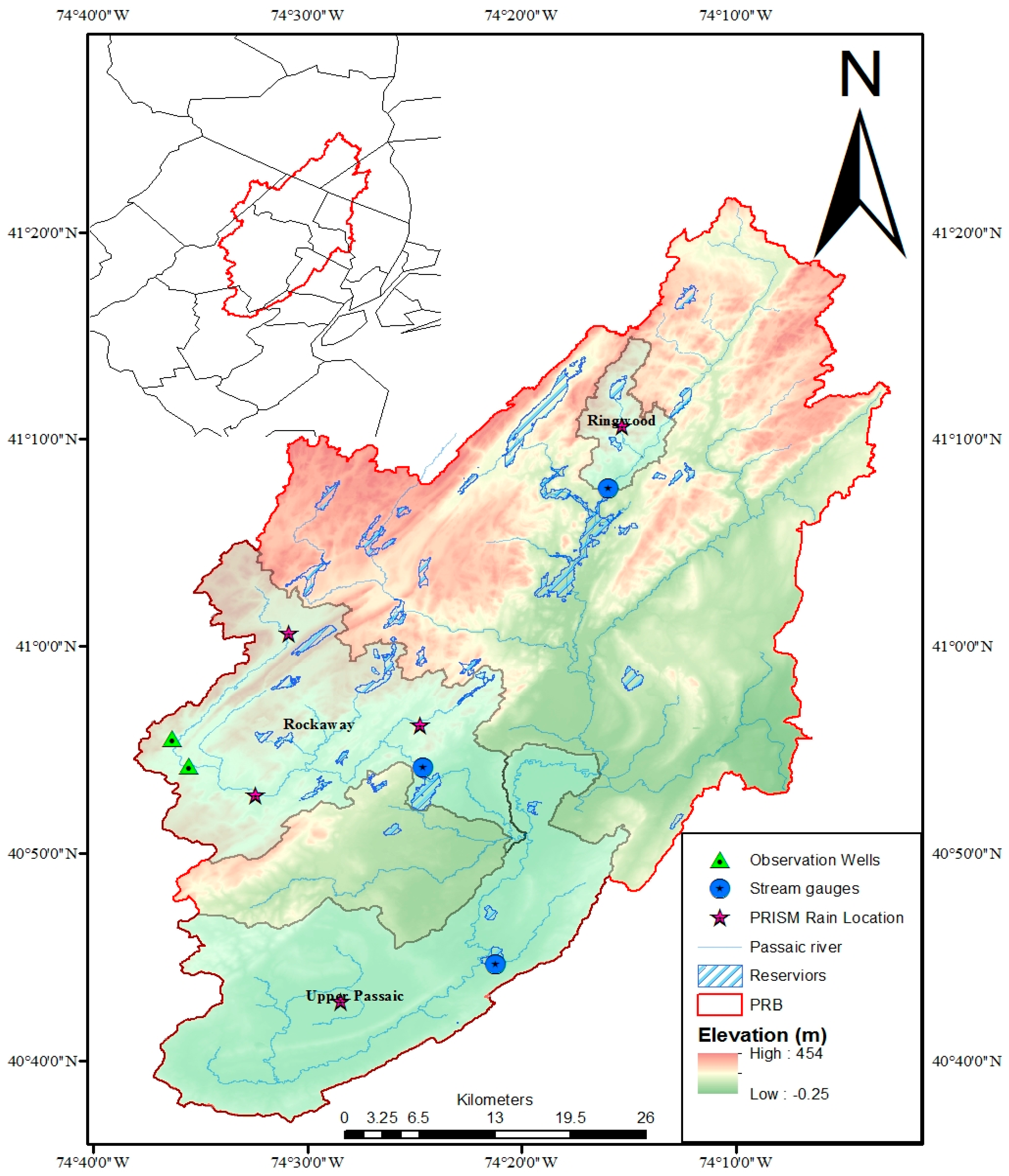
2.1. Study Area

The nontidal portion of the PRB is elliptical in shape, draining approximately 2135 square kilometers of Northern New Jersey (NJ) and Southern New York State (NY). It is bounded by longitude 74°1′1″ and 74°39′16″ W and latitude 40°35′23″ and 41°23′37″ N, intersecting six (6) counties in NJ, two (2) in NY (Figure 1). The entire basin stretches across three (3) Watershed Management Areas (WMA-03-04-06) with seven major tributaries: Whippany River, Rockaway River, Pompton River, Pequannock River, Wanaque River, Ramapo River, and Saddle River. Physiographically, the basin can be divided into three main regions: the series of parallel ridges that trend northeast/southwest forming the Highlands; the Central Basin, comprising large areas of swamps and meadows; and the roughly flat Lower Valley. Winding through seven counties and 45 municipalities, the Passaic River originates from near the Borough of Mendham (Morris County), and finally empties into the Newark Bay. The nontidal part of the river is regulated by 10 major reservoirs (Canister, Greenwood lake, Clinton, Oak Ridge, Charlotte-burg, Echo lake, Split Rock, Monksville, Wanaque, and Boonton) to provide flood control and water supply, among other things, to surrounding municipalities. Aggregated reservoir storage in the basin is about 68,533 million gallons (MG). Of the reservoirs, Wanaque reservoir is the largest, with storage capacity of 29,630 MG (43%) of the basin total (New Jersey Water Science Center, 2018; Survey, 1964, 1970; Wells, 1960). A summary of the hydrometeorological conditions in the basin is given in

Table 1. Basic hydroclimatic information in the Passaic River Basin.

	Drainage Area (sqkm)	Area (% of PRB)	Annual Flow (m3s)	Temperature (°C)	Precipitation (mm)
			Mean (Min–Max)
PRB	2135	-	402,088 (30,968–958,992)	10.59	1281
RA	300.4	14.07	2513 (611–4037)	9.52	1296
RW	46.4	2.17	337 (122–721)	9.74	1298
UP	356.3	16.67	1916 (344–2977)	11.11	1269

PRB (1983–2021 WY); RA (1971–2010 WY); RW (1986–2021 WY); UP (1971–2010 WY).

. Mean annual flow at the outlet of the basin is estimated at 402,088 m³/s for the 1983–2021 period. On average, the Rockaway river (RA) contributes about 0.62 percent of flow to the Passaic river. The study basin lies within the modified continental climate zone, characterized by hot summer and cold winter (Paulson, 1991). Moving from north to south in New Jersey, the modified climate zone comprises five (5) main divisions: North, Central, Southwest, Pine Barrens, and Coastal zones with PRB located in the North and Central climate zones. For the period 1981–2010, mean annual precipitation of 1281 mm (50.4 in) occurred over the PRB with higher values (1298 mm or 51.1 in) in the Ringwood catchment and the lower values (1269 mm or 49.96 in) in the Upper Passaic (UP) catchment. Mean temperature for same period in the study basin is calculated as 10.59 °C. Colder temperatures are observed over the RW and RA catchments whereas hotter temperatures occur in the UP area. Throughout the PRB, mean annual actual evapotranspiration is estimated to be approximately 793 mm or 31.2 in [46].

2.2. Hydrometeorological Data

For this study, the widely used gridded observations from Parameter-elevation Regression on Independent Slopes Model (PRISM, Oregon State University, http://prism.oregonstate.edu (accessed on 19 September 2022)) provided meteorological data. Flow data for the Rockaway and Upper Passaic subcatchments were obtained from records of reconstructed streamflow by [47] whereas data for the Ringwood catchment were sourced from the United States Geological Survey (USGS) water data website (USGS, https://waterdata.usgs.gov/nwis/ (accessed on 25 November 2022)).

The data used in this study spanned the periods 1979–2021 and 1981–2021 water years (WY) for the trend analysis and hydrological modelling, respectively. Missing flow data, when present, were handled based on streamflow outputs from a duly calibrated and validated hydrological model of the subcatchment [Ringwood, correlation coefficient: 0.85 and Nash–Sutcliffe: 0.71]. In all, seven (7) hydrometeorological variables (i.e., flow, m³/year, precipitation [precip, mm/year], minimum temperature [Tmin, °C], mean temperature [Tmean, °C], maximum temperature [Tmax, °C], number of days with precipitation greater that 10 mm [R10, day], and consecutive dry days [CDD, day]) for the three (3) studied subcatchments were processed and aggregated into annual time scales for the trend analysis.

2.3. Land-Use, Soil and Elevation Data

In hydrological processes, the combined effect of land cover, soil, elevation, and other catchment characteristics are reflected in the flow dynamics of river systems in a basin. The 2011 Land cover data were available from the National Land Cover Dataset (NLCD) [https://www.mrlc.gov/viewer/ (accessed on 13 July 2022)], and simplified into six (6) dominant land cover/vegetation classes (i.e., developed, forest, agricultural, wetlands, bare land, and water). Soil information was accessed using the United States Department of Agriculture (USDA) soil data viewer software [version 6.2]. The topography of the PRB was defined by a digital elevation model (DEM) extracted from the USGS database at 10 m spatial resolution (https://apps.nationalmap.gov/downloader/ (accessed on 15 May 2020)).

3. Methods

In line with the objectives of the study, two major tasks were carried out: 1) the analysis of hydroclimatic trends via the discrete wavelet transform (DWT) approach; and 2) the development of a hydrological model to assess the impacts of recent climate changes on water balance terms (i.e., precipitation, evapotranspiration, and streamflow). The hydroclimatic trend detection was conducted for seven (7) indicator variables in three (3) subcatchments because of their physiographically distinct locations. The hydrological modeling study was, however, conducted for only the Rockaway sub-basin given its relatively large size, largely representative characteristics to the PRB, and available groundwater data. Summary of the steps involved in our analyses are outlined below and described in more detail in the forthcoming sub-sections:

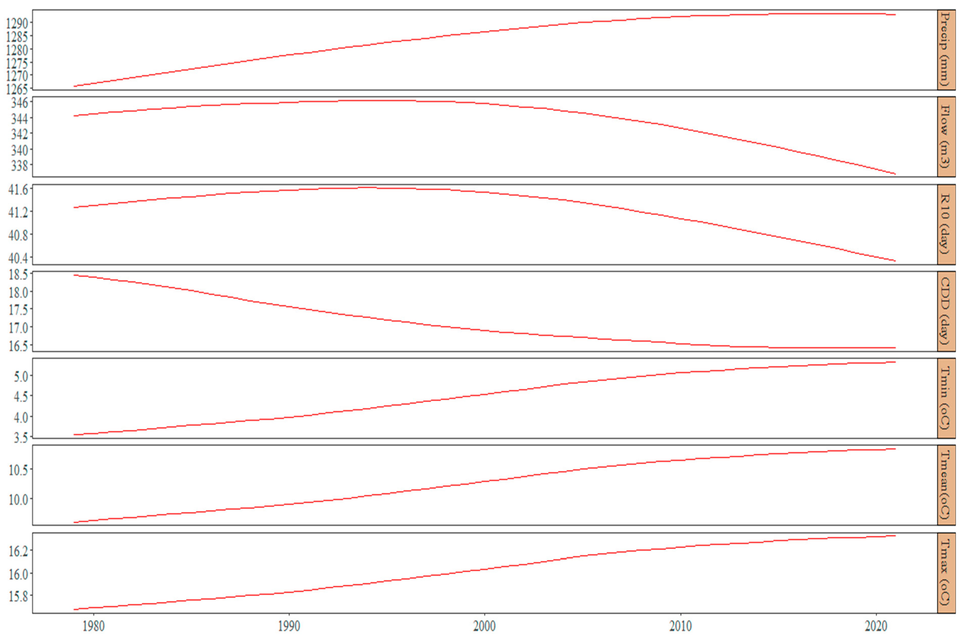
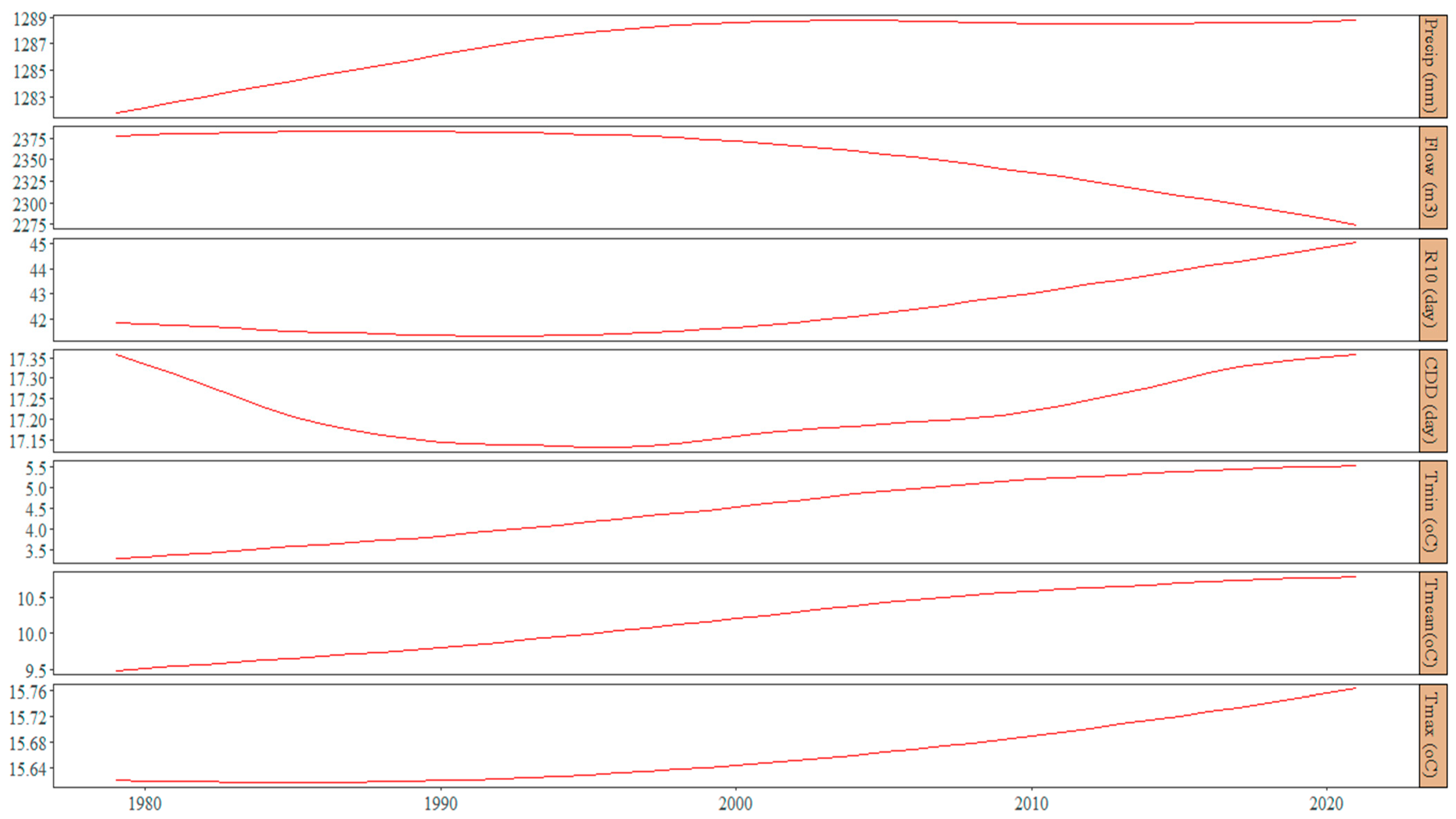
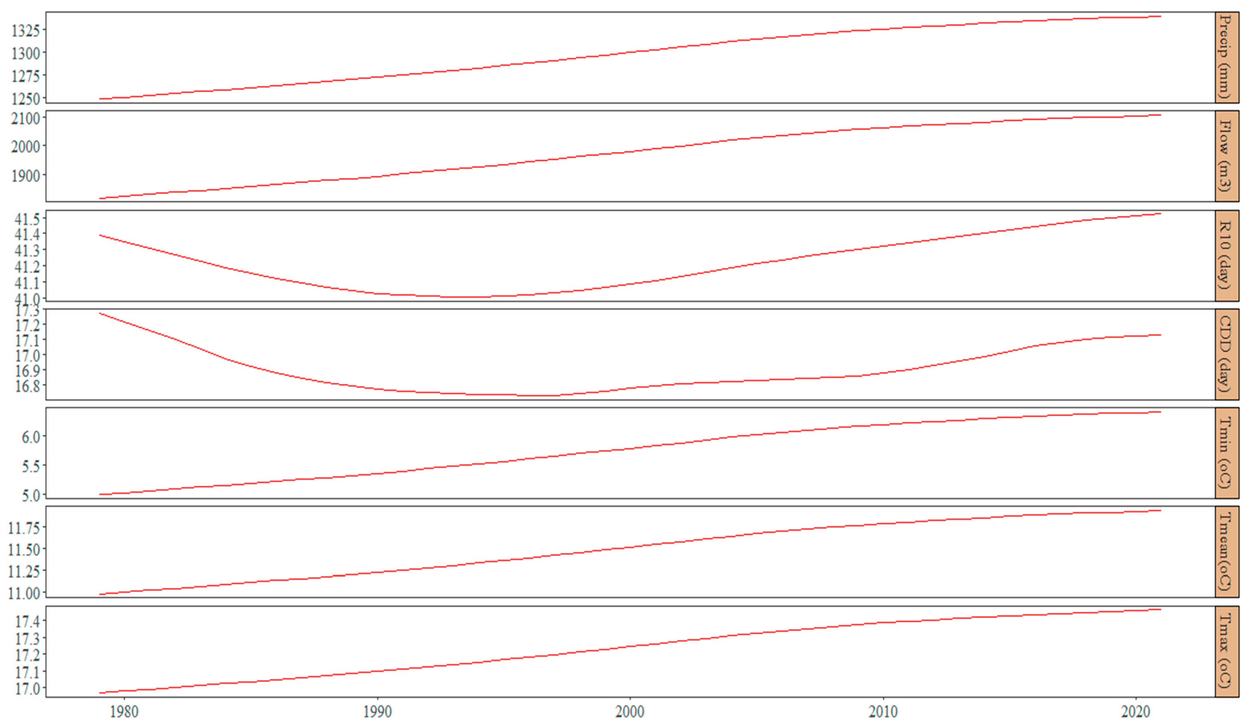
• Seven (7) different hydroclimatic indicator variables used in the trend analysis were derived from temperature, precipitation, and streamflow data series obtained for each subcatchment. They were mean annual Tmin, Tmean, Tmax, Precip, Flow, R10, and CDD spanning the period 1979–2021.
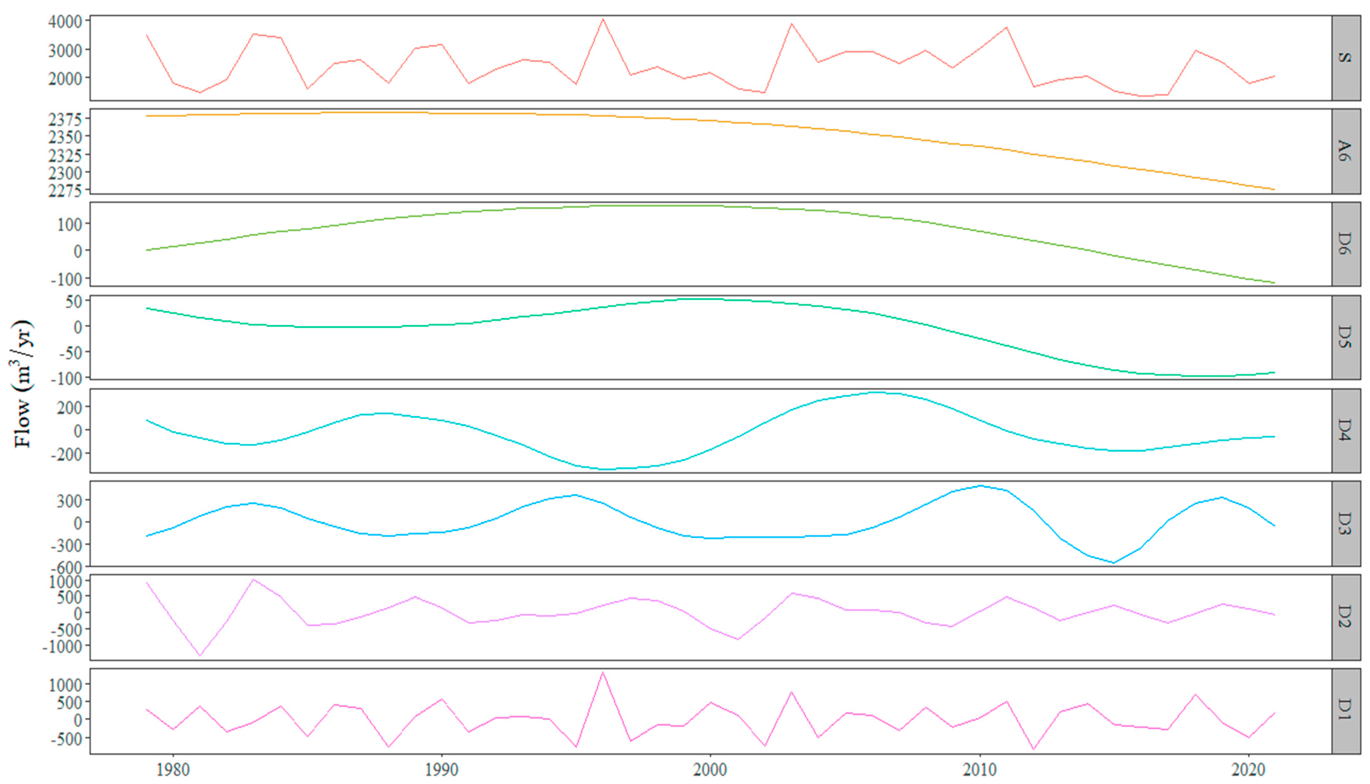
• Each time series was decomposed via the DWT, having selected the Daubechies (db) wavelet, deemed an appropriate mother wavelet in our study context, to split the series into their high frequency detailed (D) and low frequency approximate (A) components.
• The MK Z-values of the original signal and the approximation of each Daubechies (db) wavelet form starting from db4–db10 (e.g., [48]) were computed to determine the wavelet form that gives MK Z-value closer to that of the original signal. This was the optimal trend from the approximation components of each analyzed time series.
• Having selected the optimal monotonic trend, an MK test was subsequently applied to determine the statistical significance of the DWT-based trend.
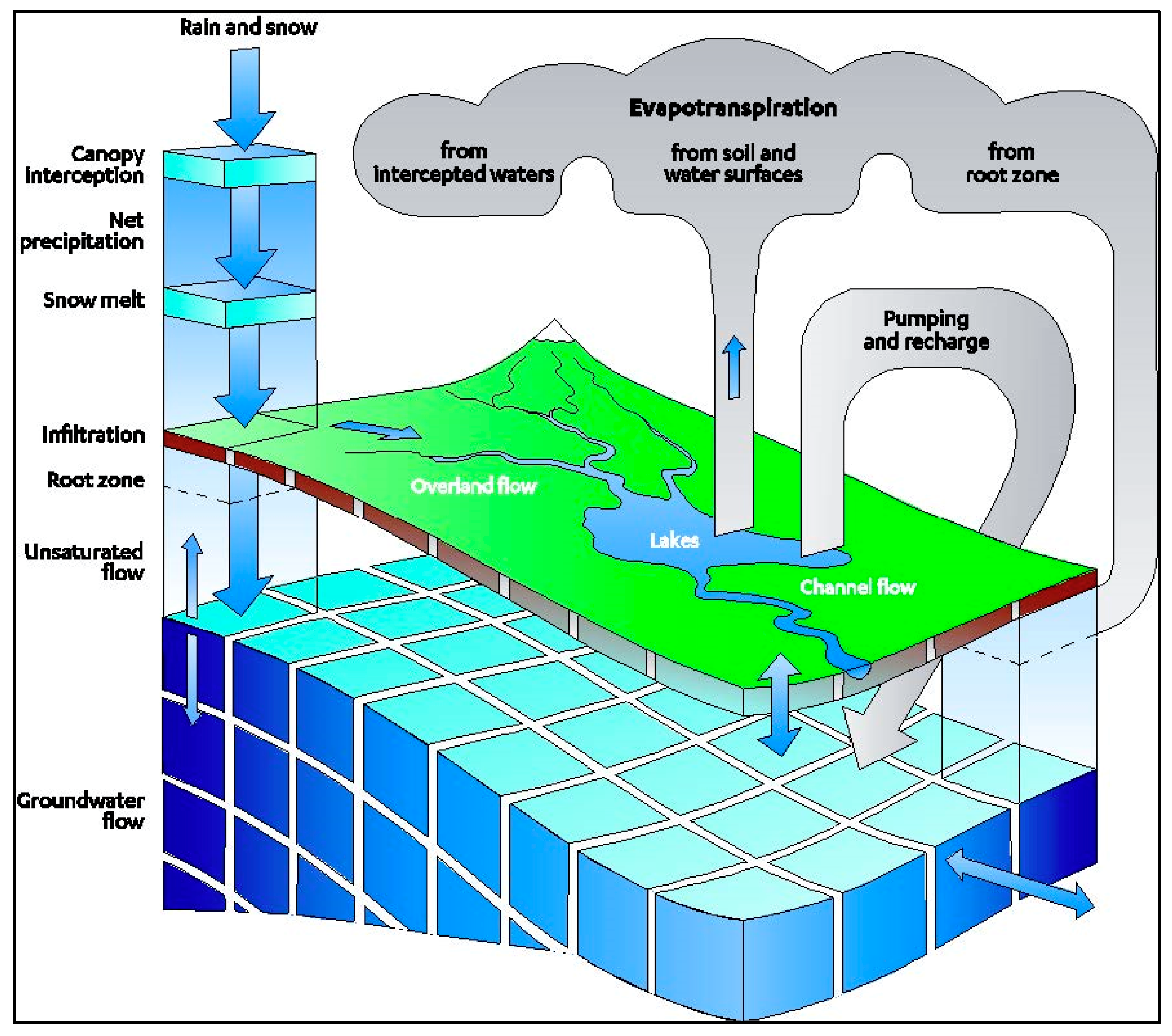
• A hydrological model for the Rockaway subbasin was developed, calibrated, and validated, and the performance of the model against the observed streamflow and groundwater data was evaluated using standard statistical criterion. The water balance module was run to obtain outputs of water-balance components for the impacts assessment.
• Change point analysis was carried out to divide data into the naturalized or baseline periods, where minimum effects of human activity on streamflow is expected and impacted periods. Subsequently, a climate elasticity exercise was undertaken to explore sensitivities of climate variables to streamflow and corresponding contributions in the Rockaway sub-basin.

3.1. Discrete Wavelet Transform

Wavelet transform (WT) is a mathematical tool that uses wave functions known as wavelets—akin to the sine and cosine functions in Fourier transforms (FT), to convert signals or time-series data into different frequency components. WT rides on the fundamental concept of Fourier transform, which operates on the idea that any function can be decomposed into a sum of pure waves with different frequencies. Therefore, the frequency domain represents the relative contributions of each frequency that comprises the function. The major limitation with FT is that knowledge about frequency is accessed at the expense of the temporal dynamics (i.e., there is no clue as to when certain frequencies begin or end). As a result, wavelets come into play to resolve this inherent trade-off of information between frequency and time in the FT [49]. Through the application of wavelet transform, an optimal frequency–time balance is attained. The key feature about wavelets is that the wave-like oscillations are short-lived and localized in time. It is worth noting that a wavelet is not just a function, but a whole family of functions which all satisfy certain requirements. The popular family of functions include Daubechies, Coiflet, Symlet, Haar, Morlet, Gaussian, Shannon, Meyer, and Mexican Hat; each one of these is tuned for specific applications. In general, to be considered a proper wavelet, a function must satisfy two main constraints: (1) the admissibility condition of having a zero mean, and (2) the finite energy condition of having a limited duration, from which a function attains its localized nature in time. In short, wavelet analysis is a completely flexible windowing technique that allows a function to change over time based on the shape and compactness of the time-series signal [50]. By this very nature, different modes of variability that varies in time can be extracted in the WT process, allowing the time-frequency characteristics of any kind of signal to be analyzed (Wei et al., 2012). Recent years have seen a wide range of studies using WT, especially to analyze hydrometeorological time-series (e.g., [29,30,51,52,53,54,55]). While the vast majority of these studies focused on trends, others emphasized the dominant periodic time scale responsible for the trends.

In the WT process, as a mother wavelet moves across the signal, several coefficients are generated according to the similarity between the signal and the mother wavelet at any specific scale. Generally, WT is divided into two main types, the continuous wavelet transform (CWT) and the discrete wavelet transform (DWT). The continuous type can generate quite numerous and often redundant coefficients at every resolution level, making its application and interpretation more complex and uncertain. The DWT is, however, considered a more effective approach, having the ability to overcome the data redundancy issue by simplifying the transformation process based on the dyadic (power of 2) scale [56]. Given a suitable wavelet family and decomposition level, the DWT decomposes a series into several sub-series during the transformation process (Whitcher et al., 2002). Following Equation (1) below (reader is referred to [56] for details), the coefficients of DWT can be calculated:

$$W_{\phi }\left(a,b\right)=\frac{1}{{\left(2\right)}^{a/2}}{{\displaystyle \sum }}_{t=0}^{N-1}X\left(t\right)\phi \left(\frac{t}{2^a}-b\right)$$

(1)

where $2^a$ denotes the dyadic scale of the DWT. Note that the resulting detail and approximation coefficients from the decomposition are merely intermediate coefficients, and has to be reconstructed, first to their approximation and detail components and then to the original signal. This readjustment to the original one-dimensional signal ensures that each component has the same length as the original signal, thereby enabling proper investigations of their contribution to the signal [57,58,59]. In a simplified form, the reconstruction of the detail and approximation components can be computed as:

$$S\left(t\right)=A_n\left(t\right)+{{\displaystyle \sum }}_{l=1}^n{D}_l\left(t\right)$$

(2)

where $S\left(t\right)$ is the original signal, and $A_n\left(t\right)$ is the approximation component at level $n$, and $D_l\left(t\right)$ is the details component at different levels (where $l$ = 1, 2, 3, …, $n$ denotes index for the levels). In MATLAB, computation of a perfect signal reconstruction is achieved using the Inverse Discrete Wavelet Transform (IDWT).

Although nearly all hydroclimatic processes are continuous in nature, their available time-series outputs are delivered in discrete formats (Wilks, 2011), making its use with DWT more appropriate than that of CWT. In the application of DWT, the original time-series signal is passed through low-pass and high-pass filters and emerge as Approximation (A) and Detail (D) components, respectively. While component D represents the small scale, high-frequency series, component A comprises the high scale, low-frequency series [34]. The decomposition process can continue iteratively, where component A from the first decomposition is further divided into new A and D components [33,49,54,60]. In this study, the Daubechies mother wavelet was chosen because of its characteristic orthogonality, and compact support, which are very important properties for localizing events in signal analysis, and deemed appropriate for hydrometeorological time-series [33,61].

Time-Series Decomposition via DWT

In our wavelet analysis, the one-dimensional flow signal (data series) and each of the temperature and precipitation indicator variables served as inputs to the multi-level 1-D wavelet decomposition function in the MATLAB Wavelet Toolbox (MATLAB version R2021a). With the db wavelet family as the mother wavelet, the operation produced a wavelet transform of each input time-series signal at all dyadic scales. Three main parameters were taken into account during the DWT process [33]: (1) the appropriate type of db wavelet; (2) a suitable signal border extension method; and (3) the most appropriate number of decomposition levels. First, several forms of db wavelet (e.g., db1–db10) exist, and the appropriate type must be selected for the decomposition process [62]. As suggested by [33], a useful method in selecting the appropriate db wavelet type is to calculate the relative error (R_E) between the MK Z-values of the original signal and that of the approximation (A) of the last decomposition level. R_E is computed as follows:

$$R_E=\frac{\left|Z_a-Z_o\right|}{\left|Z_0\right|}$$

(3)

where $Z_a$ and $Z_o$ are the MK Z-values of the approximation of the last decomposition level and the original dataset, respectively. For each indicator variable and study catchment, the appropriate db wavelet was selected to minimize $R_E$. Because trends are supposed to be gradual and slowly changing process, smoother db wavelets (i.e., db4–db10), considered as better in detecting time varying behavior over the long term [33,63], was used in the selection of the appropriate db wavelet in the study (

Table 2. Daubechies (db) wavelet type, minimum relative error (RE), Mann–Kendal test, and Sen’s slope (SS) for each metric in each subcatchment (* denotes significant at p = 0.05).

Subcatchment	Parameter	Metrics
		Precip	Flow	R10	CDD	Tmin	Tmean	Tmax
Ringwood	Wavelets	db7	db6	db8	db5	db4	db4	db4
	RE	3.75	0.03	4.86	5.72	3.93	4.48	13.46
	MKSL	871 *	−457 *	−457 *	−877 *	903 *	903 *	903 *
	SS	0.723	−0.165	−0.024	−0.051	0.047	0.033	0.018
Rockaway	Wavelets	db5	db6	db8	db4	db4	db4	db10
	RE	7.29	4.18	2.91	3.02	4.43	4.29	10.33
	MKSL	635 *	−745 *	577 *	293 *	903 *	903 *	831 *
	SS	0.129	−2.406	0.083	0.0042	0.059	0.035	0.0034
Upper Passaic	Wavelets	db4	db4	db7	db4	db4	db4	db4
	RE	7.49	6.32	67.10	7.79	3.21	3.79	6.86
	MKSL	903 *	903 *	433 *	213 *	903 *	903 *	903 *
	SS	2.401	7.712	0.0134	0.0062	0.0375	0.0253	0.013

). Second, border extension is an important consideration due to the issue of border distortions in the DWT process, arising because of the finite length of the signal. Thus, the decomposition process cannot occur outside the two limits (i.e., the start and end points) of a signal as there is no available information beyond the ends [64]. As suggested by [64], three different border extension methods are employed to address the issue: zero-padding, symmetrization, and periodic padding. In our analysis, symmetrization—which is the default mode in MATLAB, was used. It assumes that signals beyond the original support can be retrieved by symmetric boundary replication [54]. Finally, the relevant number of decomposition level must be determined in order to avoid unnecessary levels of data decomposition especially, for larger datasets (see [33,54]). This will, however, depend on the length of data points as well as the type of mother wavelet used. According to [65], the maximum number of decomposition level, $L$, can be calculated from Equation (4) below.

$$L=\frac{Log\left(\frac{n}{2v-1}\right)}{Log\left(2\right)}$$

(4)

where $n$ is the number or length of data points in the time series and $v$ is the number of vanishing moment of a db wavelet [34]. In MATLAB, the number of vanishing moments ($v$) is equal to the db wavelet type number (i.e., 1–10). Note that the number of data points ($n$) in a time series is not exactly in a dyadic format (as in the case of this study, 43 data points). Thus, the DWT computation in MATLAB is carried out using the nearest upper dyadic arrangement. Therefore, the maximum decomposition level based on our data points was calculated to be 6 in the study. Additionally, because data decomposition via DWT assumes a dyadic format, each of the decomposed component represents a different period of integer powers of two from the lowest scale. Therefore, D1, D2, and D3, respectively, represents 2-, 4-, and 8-unit periodic component, in that order, according to the time scale (e.g., seasonal, monthly, annual) used in the analysis. For example, D2 will represents a 4-year or 4-month intervals in an annual or monthly data series, respectively, but 12-month intervals for a seasonal data series since its time step is 3 months.

3.2. Trend and Change-Point Detection Tests

In this study, the Mann–Kendall (MK) test [26,35,66,67,68] was used to determine the statistical significance of the DWT-based trend [48]. It is probably the most widely used nonparametric statistical test for monotonic trend evaluation [69]; and well noted for its simplicity, robustness, and resilience to missing values in a data series [63]. One key issue that may arise when using the MK test is the presence of serial correlation or autocorrelation, very common in precipitation and streamflow data [56]. It occurs when a variable and a lagged version of itself is observed to be correlated between two successive time intervals. If the lag-1 autocorrelation in a time series is found to be significant, the modified MK test must be used [70]. Although autocorrelation issues are not common in annual data series, we applied the modified version of the MK test in this study where significant lag-1 autocorrelation was detected in our data series.

Furthermore, a change-point analysis was performed to identify the most likely year(s) in our streamflow data where significant changes could occur [71,72]. This was key in our hydrological impacts analysis where we needed to explore naturalized periods when stream flow experienced little or no disturbance as well as impacted periods. Various change-point methods exist, including the sequential Mann–Kendal test [73], Pettit’s test [74], the cumulative sum (CUSUM) test [75], and the Worsley Likelihood Ratio Test [76]. Using the R packages changepoint and ecp [77], the distribution free CUSUM test [78] and the complementary Permutation test [79] were used because they revealed similar break-point years in our streamflow time-series. These methods detect significant changes in the mean or distribution of a time series when the exact times of the changes are not known. For a detailed description of these methods, we refer the reader to the relevant literature cited.

3.3. Hydrological Model Development for the Rockaway River Basin

In the present study, the numerical code used for our hydrological assessment studies is MIKE SHE [80]. MIKE SHE is an integrated, fully distributed, physically based hydrological modeling system [81,82], that simulates all the major hydrologic process in the land phase of the hydrological cycle including evapotranspiration, overland flow, unsaturated flow, saturated flow, and streamflow (Figure 2). It uses the hydrodynamic model MIKE 11/MIKE Hydro to simulate channel flow and lakes (using flood code) in one dimension. For a detailed description on the development and modelling structure of the MIKE SHE hydrologic model the reader is referred to the MIKE Zero user manual by [81].

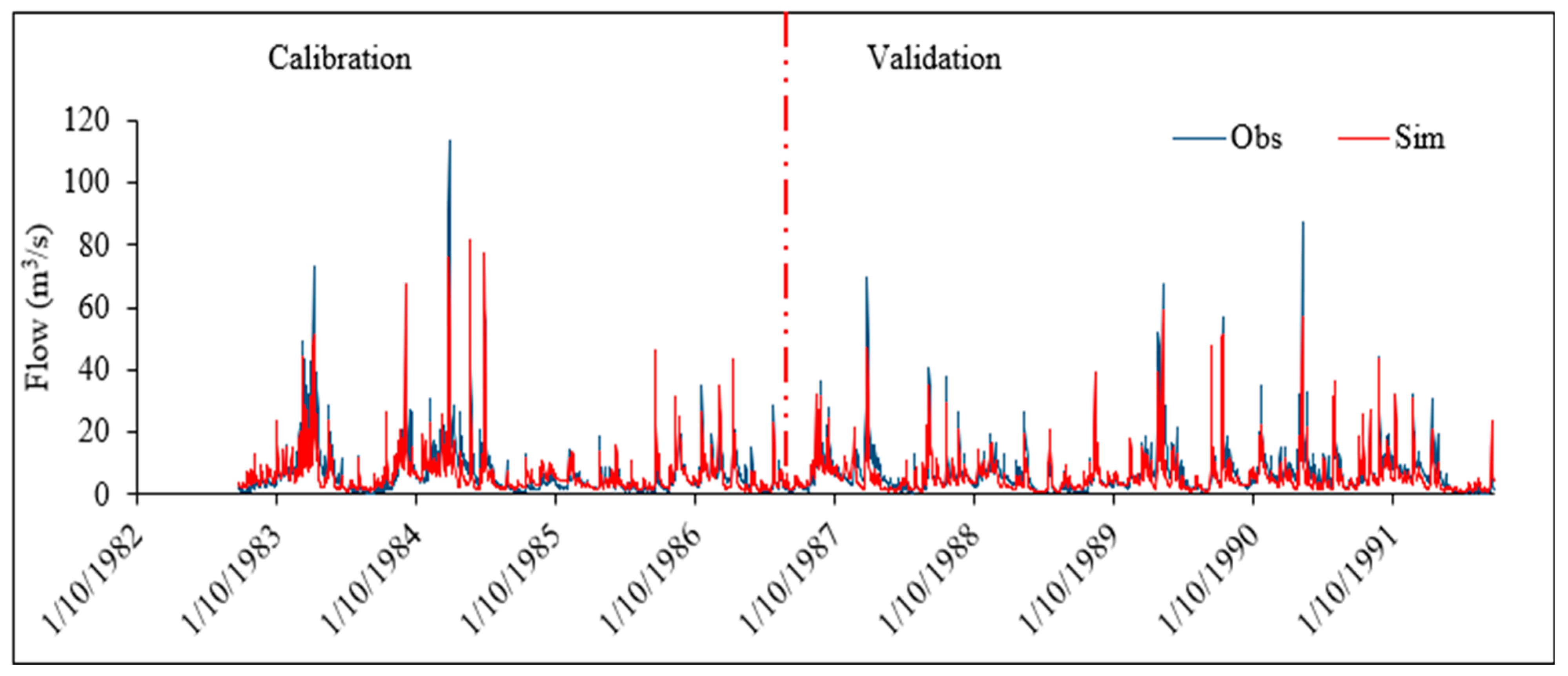
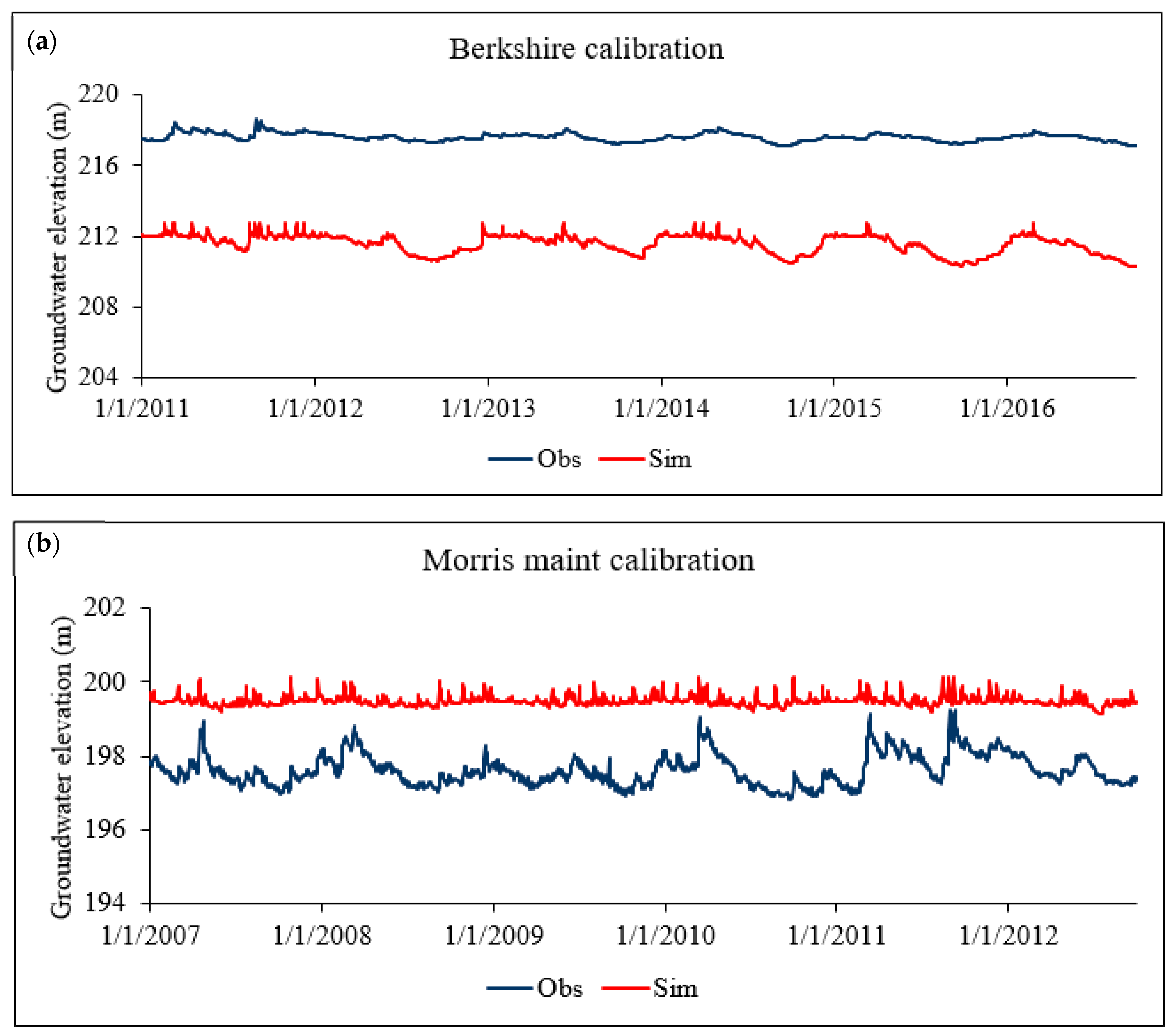
Model Calibration and Validation

A distributed hydrologic model such as MIKE SHE typically requires large number of model parameters to be assigned. Although these parameters have a clear physical meaning and can be defined explicitly from field measurements, ref. [84] suggested that the number of parameters subject to calibration should be as small as possible. For this study, initial values as well as ranges of primary parameters from field data, the published literature, and prior modelling experience guided the calibration process. The manual “trial and error” procedure was first applied, which involved perturbing one parameter while keeping all other parameters unchanged. This was carried out repeatedly within a reasonable range of values for a series of model runs until a favorable agreement between measured and simulated flow and groundwater level was achieved. Following the manual approach, an automatic calibration was conducted. Finally, validation was carried out to ensure that model parameters derived from calibration were generally valid.

Prior to the model calibration, change point analysis was performed on the streamflow data for the time span of 1981–2022 to find likely break-point year(s). Accordingly, the data were divided into baseline periods (1982–1991, 1992–2001, and 1982–2001) and impacted periods (2002–2011 and 2012–2021), as mentioned earlier. The calibration and validation of the model was carried out within the baseline period for 1982–1986 and 1986–1991, respectively. Typically, the simulation period includes the first few months of warm-up period to stabilize the model; as well as the calibration and validation periods. The adequacy of the model was evaluated based on four standard statistical criteria used in MIKE SHE: mean error (ME), root mean square error (RMSE), correlation coefficient (R), and the widely used Nash–Sutcliffe coefficient (NSE). These indicators detect system errors and the goodness of fit between simulated and observed monitoring observations in the form:

$$M{E}_i=\frac{{{\displaystyle \sum }}_t\left(Ob{s}_{i,t}-Cal{c}_{i,t}\right)}{n}$$

(5)

$$RMSE=\frac{\sqrt{{{\displaystyle \sum }}_t{\left(Ob{s}_{i,t}-Cal{c}_{i,t}\right)}^2}}{n}$$

(6)

$$R=\sqrt{\frac{{{\displaystyle \sum }}_t{\left(Cal{c}_{i,t}-{\overline{Obs}}_i\right)}^2}{{{\displaystyle \sum }}_t{\left(Ob{s}_{i,t}-{\overline{Obs}}_i\right)}^2}}$$

(7)

$$NSE=1-\frac{{{\displaystyle \sum }}_t{\left(Ob{s}_{i,t}-Cal{c}_{i,t}\right)}^2}{{{\displaystyle \sum }}_t{\left(Ob{s}_{i,t}-{\overline{Obs}}_i\right)}^2}$$

(8)

where t is the simulation time in day; n is the total simulation days; i is the calibration point i; Obs_i,t is the observed daily discharge at location i at day t; $\overline{Ob{s}_i}$ is the mean of the observed discharge at location i for the simulation period, and Calc_i,t is the simulated discharge at location i at day t.

3.4. Hydrological Impacts Assessment

After successfully calibrating and validating the hydrologic model for the period (1982–1991) considered to be within the naturalized undisturbed periods, the model was run with climatic inputs to simulate discharge for both the naturalized periods and the impacted periods identified by the change point analysis. In all, discharge for five (5) different periods were simulated, and a water balance output obtained for precipitation (P), streamflow (Q), and actual evapotranspiration (ET). Further, we assessed the hydrological impacts by computing changes between the baseline periods and impacted periods for the water balance components. Finally, the concept of elasticity as proposed by [85] was employed to evaluate the sensitivities of streamflow to changes in climate. According to this concept, climate elasticity of streamflow is the proportional change in streamflow divided by the proportional change in a climate variable. For instance, the precipitation elasticity of streamflow is defined as:

$${\epsilon }_p=\frac{dQ/Q}{dP/P}=\frac{dQ}{dP}·\frac{P}{Q}$$

(9)

Likewise, the actual evapotranspiration elasticity of streamflow is:

$${\epsilon }_{ET}=\frac{dQ/Q}{dET/ET}=\frac{dQ}{dET}·\frac{ET}{Q}$$

(10)

In applying Equations (9) and (10) to the water balance outputs obtained for the Rockaway catchment model, the relative contributions of precipitation and actual ET changes to streamflow changes can be quantified. Over the long term, the water balance model can be expressed as [86]:

$$\overline{Q}=\overline{P}-\overline{ET}$$

(11)

where $\overline{Q}$, $\overline{P}$, and $\overline{ET}$ denote long term mean values. In Equation (11), there is an implicit assumption that groundwater flow into and out of the Rockaway subcatchment cancels out and storage change over the long term is negligible.

For a largely undisturbed catchment, the changes in streamflow between two periods ($dQ$) based on Equation (11) can be estimated as:

$$dQ=d{Q}_P+d{Q}_{ET}$$

(12)

with $d{Q}_P$ and $d{Q}_{ET}$ denoting the contribution to streamflow from precipitation and actual ET, respectively. Combining Equations (9), (10) and (12), $dQ$ can be rewritten as:

$$dQ=d{Q}_P+d{Q}_{ET}=\left({\epsilon }_{P·dP/P}+ {\epsilon }_{ET·dET/ET}\right)Q$$

(13)

where $dP$ and $dET$ are changes in precipitation and actual evapotranspiration between two periods. ${\epsilon }_p$ and ${\epsilon }_{ET}$ are precipitation elasticity and actual evapotranspiration elasticity of streamflow, respectively. According to [87], a 1% change in P or ET triggers an ${\epsilon }_p$ or ${\epsilon }_{ET}$ percent change in Q.

Note that flow data used in this analysis form part of the reconstructed streamflow records by [47] for selected watersheds in the PRB, and therefore the Rockaway subcatchment is assumed to be largely undisturbed for the purpose of this study. Being mindful of the fact that climate elasticity to streamflow varies depending on the location and reference period [88], we explored the sensitivities of flow relative to different baseline periods. Thus, Equation (13) was set up for the two impacted periods (2002–2011 and 2012–2021) relative to three baseline periods (i.e., 1982–1991, 1992–2001, and 1982–2001). The values of ${\epsilon }_p$ and ${\epsilon }_{ET}$ were then computed simultaneously from two equations to obtain the contributions of P and ET changes to streamflow change in the Rockaway subbasin.

4. Results and Discussion

4.1. Decomposition of Time-Series Data via DWT

According to Equation (3), the types of db mother wavelet that produced the optimal parameters for the decomposition process for each dataset are presented in Table 2. Figure 3 illustrates an example of the decomposition results for the flow data in the Rockaway subcatchment. The original time series or signal (S) can be reconstructed by summation of all the detailed components (D1–D6) and the approximation component of the last decomposition level (A6). It can be seen that at higher decomposition levels, the frequency of the D components decreases. The last decomposition level of the A component (A6) shows the trend of streamflow in the Rockaway catchment. On a dyadic scale, D1 depicts the time series of a 2-year mode, D2 shows a 4-year mode, D3 is in an 8-year mode, D4, a 16-year mode, D5 corresponds to a 32-year mode, and 64-year mode for D6. These modes are the time scales at which those cycles are revealed, implying that for a dataset spanning a period of 42 years, the trend as revealed by the DWT for stream flow in the Rockaway catchment could only emerge over a 64-year cycle. It was thus impossible to see this trend just by applying the MK trend test on the raw dataset. The same process was replicated in all three subcatchments for each hydroclimatic indicator variable, as depicted by Figure 4, Figure 5 and Figure 6. At a confidence level of 95% (i.e., p-value = 0.05), MK statistics were subsequently applied to the decomposed times series.

4.1.1. DWT Trend Analysis of Hydroclimatic Indicators

Results from the trend analysis using the discrete wavelet transform for Precip, Flow, R10, CDD, Tmin, Tmean, and Tmax from the Ringwood, Rockaway, and Upper Passaic catchments are shown in Figure 4, Figure 5 and Figure 6. Mann–Kendall statistics (i.e., significant level (SL) and Sen’s slope (SS)) applied on the DWT trend results are also summarized in Table 2. The positive and negative MK values indicate significantly increasing and decreasing trends, respectively, and the magnitude of the trends is described by the SS values. All the analyzed hydroclimatic signals were significant at p = 0.05, identified by the asterisk.

4.1.2. Hydroclimatic Trends in the Ringwood, Rockaway, and Upper Passaic Subcatchments

DWT trend results for all hydroclimatic variables in the Ringwood subcatchment are shown in Figure 4. Precipitation shows a significant increasing signal at a rate of 0.723 mm/year. However, this increase does not reflect in the streamflow trend in the Ringwood subcatchment. Flow is rather showing a significant downward trend beginning from 1996 through to 2021 at a rate of 0.165 m³yr⁻¹. It does appear that the downward trend observed for streamflow largely tracks with heavy precipitation (R10) rather than mean precipitation, and corroborated by the decreasing trend in consecutive dry days (CDD). The observed significantly increasing trend in minimum, mean, and maximum temperatures suggest that temperature drives the flow dynamics in the Ringwood subcatchment with minimum temperature having the highest magnitude at 0.047 °Cyr⁻¹ and maximum temperature having the least at 0.018 °Cyr⁻¹.

Long-term trends in hydroclimatic indicator variables in the Rockaway catchment are illustrated in Figure 5. Similar to the Ringwood subcatchment, precipitation and streamflow are trending in opposite directions. As precipitation trends upward, flow is trending downward at rates of 0.129 mmyr⁻¹ and 2.406 cmyr⁻¹, respectively. Quite interestingly, a significantly upward trend is observed for heavy precipitation, in line with mean precipitation, yet these increases do not reflect in the observed flow trend. Given that consecutive dry days show a significantly increasing trend in tandem with minimum, mean, and maximum temperatures, there is a likelihood that precipitation is overwhelmed by relatively high temperatures in the Rockaway subcatchment, thereby translating in the observed downward trend in streamflow.

Figure 6 shows the hydroclimatic trends in indicator variables for the Upper Passaic subcatchment. All the metrics showed significantly increasing trends over the period. The observed upward trend in mean and heavy precipitation in the same direction as flow and temperatures indicate that the hydrology of the Upper Passaic subcatchment is largely driven by precipitation rather than temperature. Precipitation and flow are increasing at a rate of 2.401 mmyr⁻¹ and 7.712 cmyr⁻¹, respectively. In the case of temperature, the rate is higher in the minimum temperature (0.038 °Cyr⁻¹), followed by the mean temperature (0.025 °Cyr⁻¹) and maximum temperature (0.013 °Cyr⁻¹) (Table 2).

4.1.3. Comparison of Hydroclimatic Trends by Catchment

Trending from north to south of the PRB, the results suggest that hydroclimatic indicator variables are spatially nonuniform in terms of magnitude and direction. Over the analyzed period (1979–2021), precipitation is observed to show increasing signals in all subcatchments. Relatively, the rate of change is observed to be rapid in the Upper Passaic subcatchment at 2.401 mmyr⁻¹ and smooth in the Rockaway subcatchment at 0.129 mmyr⁻¹. Likewise, temperatures also show significantly upward trends in all subcatchments, with mean temperature displaying the highest rate of change in the Rockaway subcatchment, followed by Ringwood, and Upper Passaic subcatchments. The observed long-term increasing trend in precipitation and temperature in the PRB is indicative of a changing climate in the basin, consistent with the dominant trends in the broader Northeast United States region (e.g., [89,90]). In terms of extremes, precipitation intensity (R10) and consecutive dry days (CDD) point towards an upward trend from north to south in the PRB, beginning from Ringwood subcatchment with a decreasing signal to increases in the Rockaway and Upper Passaic subcatchments. This observed increasing trend is also consistent with patterns in rainfall intensity in the Northeast (e.g., [91,92]), and provides further evidence to the linkage between extreme weather events and climate change.

In the case of streamflow, the results suggest that flow patterns appear to be influenced both by surface characteristics and climate in the PRB. Although trends in precipitation and temperature are observed to increase throughout the basin, the dynamics on streamflow is different, with downward trends observed in the Ringwood and Rockaway subcatchments and an upward trend seen in the Upper Passaic subcatchment. Given that Ringwood and Rockaway subcatchments lie in the mountainous heavily forested Highlands region as against the Upper Passaic in the densely populated, highly industrialized urban belt, the observed trends are not surprising. With regards to attributing causes of streamflow changes in the PRB, the sections that follow, involving the hydrological modeling study using the Rockaway subbasin as a case study, is expected to provide sufficient clues on the driving mechanism behind the flow dynamics in the study basin.

4.2. Change Point Analysis and Calibration and Validation of MIKE SHE Model

Change Point Detection

For the purpose of the hydrological impact assessment, change point detection was carried out to determine approximate years of abrupt changes in hydroclimatic time-series.

As presented in

Table 3. Estimated break point years in precipitation and streamflow in the Rockaway subcatchment (α = 0.05).

	Cumulative Sum Test	Permutation Test
Variables	Break Point	Break Point
Precipitation	1980	1979
	1990	1991
	2002	2003
	2011	2012
Streamflow	1980	1979
	1990	1991
	2002	2003
	2011	2012

, precipitation and streamflow time-series were explored in the Rockaway subcatchment using the CUSUM test as well as the permutation test, and were significant at α = 0.05. Given that river flow in the PRB is largely regulated, the similarities as revealed by the break point years for both precipitation and streamflow seem to corroborate the findings by [93] that climate change signals are apparent in both regulated and natural river systems. Following from this, the causes of streamflow were explored by examining outputs of water balance terms from the hydrological model developed for the Rockaway subcatchment. Accordingly, we performed decadal changes in water balance terms in line with the break point years given in Table 3. Over the study period (1979–2021), decades 1 and 2 spanned the periods 1982–1991 and 1992–2001, respectively, representing baseline periods 1 (BLP I) and 2 (BLP II). The overall period from 1982–2001 was also considered, denoting baseline period 3 (BLP III). For the impacted periods, 2002–2011, and 2012–2021, respectively, represents decades 3 (D III) and 4 (D IV).

4.3. Calibration and Validation of Rockaway Model

The Rockaway model was calibrated using both streamflow and groundwater level data. The full model simulation spanned the period 1981–1991 for streamflow and 2005–2016 for groundwater flow. Observed streamflow was calibrated and validated at the outlet of the Rockaway catchment along with two (2) groundwater observation wells (located in the catchment. These two wells are approximately 2.6 km apart with Berkshire Valley well having elevation of 222 m and that of Morris Maint well, 203.4 m. As shown in

Table 4. Performance criterion of calibrated and validated MIKE SHE model at the Rockaway subcatchment.

		Streamflow			Groundwater
Statistics		Calibration	Validation	Full Simulation	Berkshire Obs Well	Morris Obs Well
		1982–1986	1987–1991	1982–1991	2011–2016	2007–2012
Correlation coefficient (R)		0.85	0.87	0.85	0.83	0.28
Nash efficiency (R2)		0.72	0.71	0.72	-	-
ME		0.57	1.34	0.96	6.01	−1.86
RMSE		4.78	3.89	0.85	6.07	1.91

and Figure 7, the performance of the model was assessed using a combination of statistical indicators and graphical representation, respectively. Generally, the model can be said to have captured the evolution of the observed flow sufficiently well, with few mismatches in peak flows likely due to the gridded structure of the forcing data. Rising limbs of hydrographs and baseflow were also reasonably simulated. The resulting correlation coefficient (R), Nash–Sutcliffe (NSE), mean error (ME), and RMSE values for both calibration and validation periods are shown in Table 4. In respect of coefficient (R), Nash–Sutcliffe (NSE), the performance of the Rockaway model can be judged according to the general performance ratings as recommended by [94] (

Table 5. General range of model performance statistics [94].

Performance Indicator	Excellent	Good	Fair	Poor
Nash-coefficient (NSE)	>0.85	0.65–0.85	0.5–0.65	<0.5
Correlation coefficient (R)	>0.95	0.85–0.95	0.85–0.75	<0.75

).

In the groundwater level simulation, the transient dynamics of water level were satisfactorily simulated for the Berkshire Valley well, but poor in the Morris Maint well (Figure 8). Aside from possible errors from the DEM, the observed bias could be linked to boundary conditions at the border that favored the Berkshire Valley well more than the Morris Maint well. Although individual biases such as this are inevitable, the multiple mode of calibration (i.e., using both streamflow and groundwater data) in this study allows for simultaneous optimization of model parameters to ensure proper balance between the two solutions (i.e., simulated hydrograph and groundwater level dynamics). Thus, in general, the MIKE SHE performed reasonably well in capturing the observed streamflow and groundwater levels in the Rockaway subcatchment. On the basis of these results, we explore and quantify the possible mechanisms behind the observed streamflow changes in the sub-basin.

Relative to the three different naturalized and baseline periods (i.e., 1982–1991, 1992–2001, and 1982–2001), decadal changes in hydrometeorological variables were computed from the impacted periods (i.e., 2002–2011 and 2012–2021) (

Table 6. Mean annual changes in climatic and streamflow variables of the Rockaway subbasin for the baseline (BLP) and impacted periods (D).

Period	Tmin (°C)	Tmean (°C)	Tmax (°C)	Precip (mm)	Evapo (mm)	Flow (m3)
BLP I: 1982~1991	2.76	9.27	15.78	1306	805	2244
BLP II: 1992~2001	2.99	9.40	15.82	1208	777	1898
BLP III: 1982~2001	2.87	9.34	15.80	1257	791	2071
D III: 2002~2011	4.31	10.09	15.89	1427	826	2277
D IV: 2012~2021	5.24	10.56	15.88	1282	837	1947
D III minus BLP I	1.55	0.82	0.11	9.29%	2.58%	1.46%
D IV minus BLP I	2.49	1.29	0.11	−1.83%	3.98%	−13.22%
D III minus BLP II	1.32	0.69	0.07	18.13%	6.25%	19.94%
D IV minus BLP II	2.25	1.16	0.07	6.11%	7.71%	2.59%
D III minus BLP III	1.44	0.75	0.09	13.54%	4.38%	9.93%
D IV minus BLP III	2.37	1.23	0.09	1.99%	5.81%	−5.97%

).

4.3.1. Hydroclimatic Response to Changes Relative to 1982–1991 Baseline, BLP I

Decadal changes (i.e., 2002–2011 and 2012–2021) in Tmin, Tmean, and Tmax for the impacted periods relative to the reference showed increase in both decades, with the recent decade (D IV) being the warmest (Table 6). Compared to mean and maximum temperatures, minimum temperature is observed to have a higher increasing rate (2.49 °C/decade), and is indicative of a rapidly warming climate in the basin. Along with the increasing temperatures, actual ET is also observed to increase in both decades (2.58% and 3.98% for D III and D IV resp.). However, precipitation is observed to increase in D III but decreased in D IV. This decrease in precipitation, though marginal, suggests that the recent decade (D IV) experienced meteorological stressed conditions with respect to the baseline and as compared to D III. Typically, evapotranspiration is limited in such water stress conditions, and is therefore expected to decline in D IV. However, a decreased precipitation not resulting in a decreased ET for D IV suggests that the rapid warming observed in the area somewhat played a key role in the increased actual evapotranspiration. This partly explains why streamflow declined disproportionately in the recent decade.

4.3.2. Decadal Changes in Hydrometeorological Variables

At a glance, the observed increase in precipitation in D III by 9.29% resulting in an increase in flow by 1.46%, and a decrease in precipitation in D IV by 1.83% leading to a decrease in streamflow by 13.22% may lead one to conclude that precipitation is the main climatic factor for streamflow changes in the basin. However, recourse to the elasticity of climate variables to streamflow in the basin will lead to a different conclusion. In

Table 7. Annual streamflow elasticities and contribution of precipitation and actual ET to streamflow changes for respective baseline periods.

		Elasticity (ε)
Period	Contribution to Q Change	Precip	Evapo	Equation
I: 2002~2011
		0.96	−2.88
	relative to BLP I	100%	~	$9.29{\epsilon }_p+2.58{\epsilon }_E=1.46$
		1.35	−0.74
	relative to BLP II	100%	~	$18.13{\epsilon }_p+6.25{\epsilon }_E=19.94$
		1.19	−1.44	~
	relative to BLP III	55%	−30%	$13.54{\epsilon }_p+4.38{\epsilon }_E=9.93$
II: 2012~2021
		0.96	−2.88
	relative to BLP I	13.28%	86.62%	$1.83{\epsilon }_p-3.98{\epsilon }_E=13.22$
		1.35	−0.74
	relative to BLP II	100	~	$6.11{\epsilon }_p+7.71{\epsilon }_E=2.59$
		1.19	−1.44
	relative to BLP III	~	100%	$1.99{\epsilon }_p+5.81{\epsilon }_E=-5.97$

, we find that elasticities of precipitation and actual ET are 0.96 and −2.88, respectively. This suggests that a 10% increase in precipitation results in a 9.6% increase in streamflow, while a 10% increase in actual ET leads to a 28.8% decrease in streamflow. Thus generally, streamflow is less sensitive to precipitation for the reference period. These elasticities also explain the relatively modest (1.46%) increase in streamflow for the 9.29% increase in precipitation in D III, and likewise the 13.22% decrease in flow for an only 1.83% decrease in precipitation in D IV with respect to the 1982–1991 baseline period. Thus, it can be concluded from the above results that actual evapotranspiration is the main climatic factor responsible for streamflow dynamics in the Rockaway sub-basin for this reference period. Although this conclusion holds true, in respect of the actual contribution to the observed streamflow changes for D III, precipitation was entirely responsible with 100% contribution. This means that the amount of precipitation was more than sufficient to satisfy evaporative demands, with the left over going into streamflow generation. For D IV, the impact of actual ET sensitivity to streamflow was largely felt. Such that, while actual ET contributed to approximately 87% of streamflow, precipitation contributed only 13%.

4.3.3. Hydroclimatic Response to Changes Relative to 1992–2001 Baseline, BLP II

Relative to the 1992–2001 reference period, all temperature variables in the basin saw increases consistent with global trends [44,95], with minimum temperature showing the largest increase in D IV (2.25 °C/decade). Unsurprisingly, actual ET followed along with temperature, with increases of 6.25% and 7.71% for D III and IV, respectively. However, these increases were overwhelmed by the respective 18.13% and 6.11% increase in precipitation, leading to a rise in streamflow by 19.94% and 2.59% for D III and IV, respectively (Table 6). Here D III, having precipitation increase by 18.13% can be considered as a meteorologically wet decade compared to D IV and relative to the baseline period. While water limits ET values in dry conditions, energy limits ET values in wet conditions [96,97]. Similarly, actual evapotranspiration in D III was largely energy-limited, leading to a considerable streamflow generation by 19.94%.

In terms of sensitivity to streamflow, Table 7 shows that streamflow elasticity to precipitation is 1.35, indicating that a 10% rise in mean annual precipitation results in a 13.5% increase in streamflow. On the other hand, streamflow elasticity to actual ET is −0.74, which suggests a 7.4% decline in streamflow for a 10% increase in actual ET. This indicates that streamflow is more sensitive to precipitation than actual ET for this reference period and that evaporative demand was overcome by the relative increases in precipitation for D III and IV. As such, the observed increases in streamflow for both decades can be entirely attributed to precipitation as revealed in Table 7.

4.3.4. Hydroclimatic Response to Changes Relative to 1982–2001 Baseline, BLP III

Minimum, mean, and maximum temperatures showed increases in both decades (D III and D IV) relative to the baseline (Table 6). With the recent decade being the warmest in the basin, minimum temperature is observed to have the highest increasing rate (2.37 °C/decade), followed by mean temperature (1.23 °C/decade), and then maximum temperature (0.09 °C/decade). Similarly, precipitation was observed to increase in both decades, with the largest increase in D III, having 170 mm (13.54%) more than in the baseline period. Consistent with temperature, actual evapotranspiration was observed to increase in both decades compared to the baseline. Although the results in Table 6 show that both precipitation and evapotranspiration are increasing for all decades relative to the baseline, they induced varied signal and strength in streamflow. Whereas precipitation was the dominant contributor to streamflow in D III (55%) leading to an increased flow, actual ET entirely overwhelmed precipitation in D IV causing a decrease in flow. The reason for this is that in D III, water was sufficient, and energy becomes the more important control of evapotranspiration whereas in D IV, water was limited, and evapotranspiration, largely driven by energy, went into further decreasing streamflow (−5.97%).

This is confirmed by sensitivity results in Table 7. It reveals that, elasticity of streamflow in relation to precipitation (${\epsilon }_p$) and actual ET (${\epsilon }_{ET}$) for the Rockaway sub-basin are 1.19 and −1.44, respectively. This indicates that 10% increase in precipitation results in 11.9% increase in streamflow while 10% increase in actual ET would lead to 14.4% decrease in streamflow. Thus, annual streamflow was generally more sensitive to the change in actual ET than the change in precipitation, although in D III, precipitation contributed 55% to streamflow changes whereas evapotranspiration contributed 30%.

5. Summary and Conclusions

At a time when the climate change problem has evolved into a crisis, the piece-meal approach to carrying out hydrological impact analysis at a single study location may no longer suffice. At best, a comprehensive study that combines the detection and analysis of trends along with hydrological modelling study will provide important foundations for understanding the hydroclimatic patterns in an area and the driving mechanisms behind these trends in the wake of a changing climate. In this study, we used long-term meteorological and hydrologic observations to identify trends in hydroclimatic indicator variables in the PRB. We also modelled streamflow and groundwater elevation using the Rockaway sub-basin as a case study to understand the impacts of recent climate changes to streamflow in the study basin. Recognizing that hydroclimatic variables, by their nature, are nonmonotonic, we employed the wavelet transform—an advanced trend analysis tool—as against the frequently used MK trend test, to detect and identify patterns in hydroclimatic variables in the PRB. Rather than using the MK trend test directly on the raw data whose results tend to be largely statistically insignificant in respect of precipitation data, for instance, the wavelet transform approach was applied to identify the hidden monotonic trends in the characteristically noisy hydroclimatic time-series. For the hydrological impact assessments, the physically based distributed MIKE SHE hydrologic model provided the platform to successfully simulate the hydrologic conditions of the Rockaway catchment. Based on the model’s water balance outputs, the impacts of recent climate were assessed from changes in naturalized or baseline periods against impacted periods. Further analysis was carried out using climate elasticities to determine the sensitivities and contributions of climatic variables to streamflow changes in the sub-basin to three different baseline conditions. By this, we demonstrated that the time perspective or baseline condition used to assess climate change impacts can also substantially influence results.

Major sources of uncertainty in this study may be that which pertains to hydrological modelling such as input, output, structural, and parametric uncertainties [98,99]. Because streamflow observations used in calibrating and validating the MIKE SHE hydrological model was based on reconstructed data, it is likely that errors emanating from the methods and data used in estimating daily reconstructed streamflow for the Rockaway catchment (refer to [47]) may be propagated in this study. Howbeit, conscious effort was made in minimizing uncertainties in our analyses first by the use of multiple objective function (i.e., observed streamflow and groundwater-level data) that allowed for simultaneous optimization of model parameters. The model’s ability to reasonably simulate both surface and subsurface flows as evidenced in the satisfactory performance criterion give credence to the findings in the study. In addition, one uncertainty that has almost been universally overlooked in climate impact studies is the choice of baseline condition. In our study, we assessed the hydrologic response to changes in climate using three different baseline climates against two recent future periods (i.e., 2002–2011, 2012–2021). We found that the choice of baseline condition constitutes an important source of uncertainty in the sensitivities of streamflow to precipitation and evapotranspiration changes and should routinely be considered in any climate impact assessment. Against this background, we present the key findings from our results below:

(1)

Over the period 1979–2021, minimum, mean, and maximum temperatures showed significantly upward trend in all studied subcatchments of the PRB with minimum temperature having the highest rate of change at 0.059 °Cyr⁻¹ in the Rockaway sub-basin. In contrast, maximum temperatures experienced the slowest rate of change at 0.0034 °Cyr⁻¹. Across the PRB, the rate of change in mean temperature ranges from 0.025–0.035 °Cyr⁻¹.

(2)

Overall, precipitation showed a significant increasing signal in all analyzed sub-basins with the fastest rate of 0.72 mm/yr in the Ringwood catchment and the slowest rate at 0.13 mm/yr in the Rockaway catchment. This observed long-term increasing trend in precipitation and temperature in the PRB is indicative of a changing climate, consistent with the dominant trends in the broader Northeastern region. Spatially, trends in both precipitation intensity (R10) and consecutive dry days (CDD) were observed to decrease in the uppermost portion of the PRB at the Ringwood catchment but increases towards the south in the Rockaway and Upper Passaic sub-basins. This pattern is also dominant in the wider Northeast, and provide further evidence of the connection between extreme weather events and climate change.

(3)

In two out of the three analyzed sub-basins, streamflow displayed significantly downward trends with an increasing trend in the Upper Passaic subcatchment. This is in spite of the increasing trends in both precipitation and temperature in all the three subcatchments. Although it is well established that precipitation amounts and intensity directly affect streamflow [100], the present results rather show that an increase in precipitation does not always lead to an increase in streamflow. From a hydrological modeling standpoint, attempt was therefore made to examine the causes of streamflow in the PRB using the Rockaway subcatchment as a case study.

(4)

Decadal changes in climate revealed that the recent decade (2012–2021) was both the warmest and driest period relative to all baseline periods, and compared with the 2001–2011 decade. It showed a mean temperature increase ranging from 1.16 °C in BLP II and 1.29 °C in BLP I. Being the driest period, the recent decade also showed precipitation changing from −1.83% to 6.11% relative to the 1982–1991 and 1992–2001 baselines, respectively. In contrast, the wettest decade was 2002–2011 relative to all baseline periods with precipitation increase ranging from 9.29% in the 1982–1991 baseline to 18.13% in the 1992–2001 baseline.

(5)

Relative to the overall baseline period (BLP III), the warmest and the driest decade (2012–2021), having a mean temperature increase of 1.23 °C induced an actual evapotranspiration increase of 5.81% and a marginal precipitation increase of 1.99%, resulting in a 5.97% decrease in streamflow. Similarly, the wettest decade (2002–2011), with mean temperature increase of 0.75 °C relative to the overall baseline period (BPL III), induced an actual evapotranspiration increase of 4.38% and a precipitation of 13.54%, which resulted in a streamflow increase of 9.93%.

(6)

Across the three baseline periods, we found that precipitation elasticity to streamflow ranged from 0.96 to 1.35 suggesting that a 10% rise in precipitation will result in between 9.6% to 13.5% increase in streamflow in the study basin. Similarly, evapotranspiration elasticity to streamflow ranged from −2.88 to −0.74 indicating that, a 10% increase in actual ET will lead to between 28.8% to 7.4% decrease in streamflow. The relatively pronounced negative ET elasticity value also reflects the effect of warming climate in the basin. Generally, as temperature increases, ET increases and streamflow decreases. With streamflow showing high sensitivity to actual ET increases more than precipitation, it is safe to conclude that, to a large extent, actual evapotranspiration is more important in the flow dynamics of the PRB in the wake of a warming climate.

(7)

The general observation therefore is that in decades where water is available, energy limits actual evapotranspiration which makes streamflow more sensitive to precipitation increase. However, in meteorologically stressed or dry decades, water limits actual ET thereby making streamflow more sensitive to increases in actual evapotranspiration.

The application of discrete wavelet-transform analysis and process-based hydrological modeling in this study adequately captured the hydroclimatic signatures as well as hydrologic response to climate change in the PRB. A broader study in the future that incorporates how hydrologic sensitivities vary spatially across the PRB will help in further minimizing the uncertainties in climate impact assessments for the basin.

References

1. Pumo, D.; Francipane, A.; Cannarozzo, M.; Antinoro, C.; Valerio Noto, L. Monthly Hydrological Indicators to Assess Possible Alterations on Rivers’ Flow Regime. Water Resour. Manag. 2018, 32, 3687–3706. [Google Scholar] [CrossRef]
2. Naderi, M.; Sheikh, V.; Bahrehmand, A.; Komaki, C.B.; Ghangermeh, A. Analysis of River Flow Regime Changes Using the Indicators of Hydrologic Alteration (Case Study: Hableroud Watershed). Water Soil. Manag. Model. 2023, 3, 1–19. [Google Scholar] [CrossRef]
3. Rasouli, K.; Scharold, K.; Mahmood, T.H.; Glenn, N.F.; Marks, D. Linking Hydrological Variations at Local Scales to Regional Climate Teleconnection Patterns. Hydrol. Process 2020, 34, 5624–5641. [Google Scholar] [CrossRef]
4. Khan, F.; Ali, S.; Mayer, C.; Ullah, H.; Muhammad, S. Climate Change and Spatio-Temporal Trend Analysis of Climate Extremes in the Homogeneous Climatic Zones of Pakistan during 1962–2019. PLoS ONE 2022, 17, e0271626. [Google Scholar] [CrossRef]
5. Rahaman, M.H.; Saha, T.K.; Masroor, M.; Roshani; Sajjad, H. Trend Analysis and Forecasting of Meteorological Variables in the Lower Thoubal River Watershed, India Using Non-Parametrical Approach and Machine Learning Models. Model. Earth Syst. Environ. 2024, 10, 551–577. [Google Scholar] [CrossRef]
6. Banda, V.D.; Dzwairo, R.B.; Singh, S.K.; Kanyerere, T. Trend Analysis of Selected Hydro-Meteorological Variables for the Rietspruit Sub-Basin, South Africa. J. Water Clim. Change 2021, 12, 3099–3123. [Google Scholar] [CrossRef]
7. Salaudeen, A.R.; Shahid, S.; Ismail, A.; Adeogun, B.K.; Ajibike, M.A.; Bello, A.A.D.; Salau, O.B.E. Adaptation Measures under the Impacts of Climate and Land-Use/Land-Cover Changes Using HSPF Model Simulation: Application to Gongola River Basin, Nigeria. Sci. Total Environ. 2023, 858, 159874. [Google Scholar] [CrossRef]
8. Banda, V.D.; Dzwairo, R.B.; Singh, S.K.; Kanyerere, T. Hydrological Modelling and Climate Adaptation under Changing Climate: A Review with a Focus in Sub-Saharan Africa. Water 2022, 14, 4031. [Google Scholar] [CrossRef]
9. Wang, N.; Yang, J.; Zhang, Z.; Xiao, Y.; Wang, H.; He, J.; Yi, L. Analysis of Detailed Lake Variations and Associated Hydrologic Driving Factors in a Semi-Arid Ungauged Closed Watershed. Sustainability 2023, 15, 6535. [Google Scholar] [CrossRef]
10. Mahmood, R.; Jia, S.; Zhu, W. Analysis of Climate Variability, Trends, and Prediction in the Most Active Parts of the Lake Chad Basin, Africa. Sci. Rep. 2019, 9, 6317 . [Google Scholar] [CrossRef]
11. Gadedjisso-Tossou, A.; Adjegan, K.I.I.; Kablan, A.K.M. Rainfall and Temperature Trend Analysis by Mann–Kendall Test and Significance for Rainfed Cereal Yields in Northern Togo. Sci 2021, 3, 17. [Google Scholar] [CrossRef]
12. Cai, Y.; Zhang, F.; Gao, G.; Jim, C.Y.; Leong Tan, M.; Shi, J.; Wang, W.; Zhao, Q. Spatio-Temporal Variability and Trend of Blue-Green Water Resources in the Kaidu River Basin, an Arid Region of China. J. Hydrol. Reg. Stud. 2024, 51, 101640. [Google Scholar] [CrossRef]
13. Sanson, A.V.; Van Hoorn, J.; Burke, S.E.L. Responding to the Impacts of the Climate Crisis on Children and Youth. Child. Dev. Perspect. 2019, 13, 201–207. [Google Scholar] [CrossRef]
14. Ojala, M.; Cunsolo, A.; Ogunbode, C.A.; Middleton, J. Anxiety, Worry, and Grief in a Time of Environmental and Climate Crisis: A Narrative Review. Annu. Rev. Environ. Resour. 2021, 46, 35–58. [Google Scholar] [CrossRef]
15. Campbell, J.L.; Driscoll, C.T.; Pourmokhtarian, A.; Hayhoe, K. Streamflow Responses to Past and Projected Future Changes in Climate at the Hubbard Brook Experimental Forest, New Hampshire, United States. Water Resour. Res. 2011, 47, 2514. [Google Scholar] [CrossRef]
16. Sharma, S.; Swayne, D.A.; Obimbo, C. Trend Analysis and Change Point Techniques: A Survey. Energy Ecol. Environ. 2016, 1, 123–130. [Google Scholar] [CrossRef]
17. Meng, F.; Su, F.; Yang, D.; Tong, K.; Hao, Z. Impacts of Recent Climate Change on the Hydrology in the Source Region of the Yellow River Basin. J. Hydrol. Reg. Stud. 2016, 6, 66–81. [Google Scholar] [CrossRef]
18. Suhaila, J.; Yusop, Z. Trend Analysis and Change Point Detection of Annual and Seasonal Temperature Series in Peninsular Malaysia. Meteorol. Atmos. Phys. 2018, 130, 565–581. [Google Scholar] [CrossRef]
19. Citakoglu, H.; Minarecioglu, N. Trend Analysis and Change Point Determination for Hydro-Meteorological and Groundwater Data of Kizilirmak Basin. Theor. Appl. Clim. 2021, 145, 1275–1292. [Google Scholar] [CrossRef]
20. Tekleab, S.; Mohamed, Y.; Uhlenbrook, S. Hydro-Climatic Trends in the Abay/Upper Blue Nile Basin, Ethiopia. Phys. Chem. Earth 2013, 61–62, 32–42. [Google Scholar] [CrossRef]
21. Ahmad, I.; Tang, D.; Wang, T.; Wang, M.; Wagan, B. Precipitation Trends over Time Using Mann-Kendall and Spearman’s Rho Tests in Swat River Basin, Pakistan. Adv. Meteorol. 2015, 2015. [Google Scholar] [CrossRef]
22. Alhaji, U.U.; Yusuf, A.S.; Edet, C.O.; Oche, C.O.; Agbo, E.P. Trend Analysis of Temperature in Gombe State Using Mann Kendall Trend Test. J. Phys. Conf. Ser. 2018, 1734, 012016. [Google Scholar] [CrossRef]
23. Basarir, A.; Arman, H.; Hussein, S.; Murad, A.; Aldahan, A.; Al-Abri, M.A. Trend Detection in Annual Temperature and Precipitation Using Mann–Kendall Test—a Case Study to Assess Climate Change in Abu Dhabi, United Arab Emirates. Lect. Notes Civ. Eng. 2018, 7, 3–12. [Google Scholar]
24. Bezerra, J.; Júnior, C.; Lucena, R.L. Analysis of Precipitation Using Mann-Kendall and Kruskal-Wallis Non-Parametric Tests. Mercator 2020, 19, 1. [Google Scholar] [CrossRef]
25. Seenu, P.Z.; Jayakumar, K.V. Comparative Study of Innovative Trend Analysis Technique with Mann-Kendall Tests for Extreme Rainfall. Arab. J. Geosci. 2021, 14, 1–15. [Google Scholar]
26. Sa’adi, Z.; Shahid, S.; Ismail, T.; Chung, E.S.; Wang, X.J. Trend Analysis of the Variations of Ambient Temperature Using Mann-Kendall Test and Sen’s Estimate in Calabar, Southern Nigeria. Meteorol. Atmos. Phys. 2019, 131, 263–277. [Google Scholar] [CrossRef]
27. Fatichi, S.; Barbosa, S.M.; Caporali, E.; Silva, M.E. Deterministic versus Stochastic Trends: Detection and Challenges. J. Geophys. Res. Atmos. 2009, 114, 1–11. [Google Scholar] [CrossRef]
28. Lutgens, F.K.; Tarbuck, E.J. The Atmosphere: An Introduction to Meteorology; Prentice Hall: Kent, OH, USA, 2010; p. 508. [Google Scholar]
29. Sang, Y.F.; Sun, F.; Singh, V.P.; Xie, P.; Sun, J. A Discrete Wavelet Spectrum Approach for Identifying Non-Monotonic Trends in Hydroclimate Data. Hydrol. Earth Syst. Sci. 2018, 22, 757–766. [Google Scholar] [CrossRef]
30. Araghi, A.; Mousavi Baygi, M.; Adamowski, J.; Malard, J.; Nalley, D.; Hasheminia, S.M. Using Wavelet Transforms to Estimate Surface Temperature Trends and Dominant Periodicities in Iran Based on Gridded Reanalysis Data. Atmos. Res. 2015, 155, 52–72. [Google Scholar] [CrossRef]
31. Hernandez, E.; Weiss, G. A First Course on Wavelets; CRC Press: Boca Raton, FL, USA, 1996; ISBN 9780367802349. [Google Scholar]
32. Kirchgässner, G.; Wolters, J. Introduction to Modern Time Series Analysis; Springer: Berlin/Heidelberg, Germany, 2007; ISBN 9783540732907. [Google Scholar]
33. Nalley, D.; Adamowski, J.; Khalil, B. Using Discrete Wavelet Transforms to Analyze Trends in Streamflow and Precipitation in Quebec and Ontario (1954–2008). J. Hydrol. 2012, 475, 204–228. [Google Scholar] [CrossRef]
34. Abebe, S.A.; Qin, T.; Zhang, X.; Yan, D. Wavelet Transform-Based Trend Analysis of Streamflow and Precipitation in Upper Blue Nile River Basin. Reg. Stud. 2022, 44, 2214–5818. [Google Scholar] [CrossRef]
35. Nourani, V.; Danandeh Mehr, A.; Azad, N. Trend Analysis of Hydroclimatological Variables in Urmia Lake Basin Using Hybrid Wavelet Mann-Kendall and Şen Tests. Environ. Earth Sci. 2018, 77, 207. [Google Scholar] [CrossRef]
36. Das, J.; Mandal, T.; Sakiur Rahman, A.T.M.; Saha, P. Spatio-Temporal Characterization of Rainfall in Bangladesh: An Innovative Trend and Discrete Wavelet Transformation Approaches. Theor. Appl. Clim. 2021, 143, 1557–1579. [Google Scholar] [CrossRef]
37. Wu, X.; Zhou, J.; Yu, H.; Liu, D.; Xie, K.; Chen, Y.; Hu, J.; Sun, H.; Xing, F. The Development of a Hybrid Wavelet-ARIMA-LSTM Model for Precipitation Amounts and Drought Analysis. Atmosphere 2021, 12, 74. [Google Scholar] [CrossRef]
38. Karbasi, M.; Jamei, M.; Malik, A.; Kisi, O.; Yaseen, Z.M. Multi-Steps Drought Forecasting in Arid and Humid Climate Environments: Development of Integrative Machine Learning Model. Agric. Water Manag. 2023, 281, 108210. [Google Scholar] [CrossRef]
39. Labat, D. Recent Advances in Wavelet Analyses: Part 1. A Review of Concepts. J. Hydrol. 2005, 314, 275–288. [Google Scholar] [CrossRef]
40. Gardner, R.H.; Urban, D.L. Model Validation and Testing: Past Lessons, Present Concerns, Future Prospects. Models Ecosyst. Sci. 2021, 184–203. [Google Scholar] [CrossRef]
41. Kucharik, C.J.; Barford, C.C.; Maayar, M.E.; Wofsy, S.C.; Monson, R.K.; Baldocchi, D.D. A Multiyear Evaluation of a Dynamic Global Vegetation Model at Three AmeriFlux Forest Sites: Vegetation Structure, Phenology, Soil Temperature, and CO2 and H2O Vapor Exchange. Ecol. Model. 2006, 196, 1–31. [Google Scholar] [CrossRef]
42. Brydon, N.F. The Passaic River: Past, Present, Future; Rutgers Univ Press: New Brunswick, NJ, USA, 1974; ISBN 9780813507705. [Google Scholar]
43. Karmalkar, A.V.; Bradley, R.S. Consequences of Global Warming of 1.5 °C and 2 °C for Regional Temperature and Precipitation Changes in the Contiguous United States. PLoS ONE 2017, 12, e0168697. [Google Scholar] [CrossRef]
44. USGCRP. Fourth National Climate Assessment; USGCRP: Washington, DC, USA, 2018. [Google Scholar]
45. Campbell, J.L.; Ollinger, S.V.; Flerchinger, G.N.; Wicklein, H.; Hayhoe, K.; Bailey, A.S. Past and Projected Future Changes in Snowpack and Soil Frost at the Hubbard Brook Experimental Forest, New Hampshire, USA. Hydrol. Process 2010, 24, 2465–2480. [Google Scholar] [CrossRef]
46. Oteng Mensah, F.; Alo, C.A. Modeling Monthly Actual Evapotranspiration: An Application of Geographically Weighted Regression Technique in the Passaic River Basin. J. Water Clim. Change 2023, 14, 17–37. [Google Scholar] [CrossRef]
47. Hickman, R.E.; McHugh, A.R. Methods Used to Reconstruct Historical Daily Streamflows in Northern New Jersey and Southeastern New York, Water Years 1922–2010; US Geological Survey: Reston, VA, USA, 2018. [Google Scholar]
48. Adarsh, S.; Janga Reddy, M. Trend Analysis of Rainfall in Four Meteorological Subdivisions of Southern India Using Nonparametric Methods and Discrete Wavelet Transforms. Int. J. Climatol. 2015, 35, 1107–1124. [Google Scholar] [CrossRef]
49. Li, M.; Xia, J.; Chen, Z.; Meng, D.; Xu, C. Variation Analysis of Precipitation during Past 286 Years in Beijing Area, China, Using Non-Parametric Test and Wavelet Analysis. Hydrol. Process 2013, 27, 2934–2943. [Google Scholar] [CrossRef]
50. Daubechies, I. The Wavelet Transform, Time-Frequency Localization and Signal Analysis. IEEE Trans. Inf. Theory 1990, 36, 961–1005. [Google Scholar] [CrossRef]
51. Adamowski, J.; Chan, H.F. A Wavelet Neural Network Conjunction Model for Groundwater Level Forecasting. J. Hydrol. 2011, 407, 28–40. [Google Scholar] [CrossRef]
52. Adamowski, J.F. Development of a Short-Term River Flood Forecasting Method for Snowmelt Driven Floods Based on Wavelet and Cross-Wavelet Analysis. J. Hydrol. 2008, 353, 247–266. [Google Scholar] [CrossRef]
53. Chellali, F.; Khellaf, A.; Belouchrani, A. Wavelet Spectral Analysis of the Temperature and Wind Speed Data at Adrar, Algeria. Renew. Energy 2010, 35, 1214–1219. [Google Scholar] [CrossRef]
54. Nalley, D.; Adamowski, J.; Khalil, B.; Ozga-Zielinski, B. Trend Detection in Surface Air Temperature in Ontario and Quebec, Canada during 1967-2006 Using the Discrete Wavelet Transform. Atmos. Res. 2013, 132–133, 375–398. [Google Scholar] [CrossRef]
55. Partal, T.; Kahya, E. Trend Analysis in Turkish Precipitation Data. Hydrol. Process 2006, 20, 2011–2026. [Google Scholar] [CrossRef]
56. Partal, T.; Küçük, M. Long-Term Trend Analysis Using Discrete Wavelet Components of Annual Precipitations Measurements in Marmara Region (Turkey). Phys. Chem. Earth 2006, 31, 1189–1200. [Google Scholar] [CrossRef]
57. Dong, X.; Nyren, P.; Patton, B.; Nyren, A.; Richardson, J.; Maresca, T. Wavelets for Agriculture and Biology: A Tutorial with Applications and Outlook. Bioscience 2008, 58, 445–453. [Google Scholar] [CrossRef]
58. Roushangar, K.; Alizadeh, F. Identifying Complexity of Annual Precipitation Variation in Iran during 1960-2010 Based on Information Theory and Discrete Wavelet Transform. Stoch. Environ. Res. Risk Assess. 2018, 32, 1205–1223. [Google Scholar] [CrossRef]
59. Wu, D.Q.; Tan, J.; Guo, F.; Li, H.; Chen, S.; Jiang, S. Multi-Scale Identification of Urban Landscape Structure Based on Two-Dimensional Wavelet Analysis: The Case of Metropolitan Beijing, China. Ecol. Complex. 2020, 43, 100832. [Google Scholar] [CrossRef]
60. Turgay, P. Wavelet Transform-Based Analysis of Periodicities and Trends of Sakarya Basin (Turkey) Streamflow Data. River Res. Appl. 2010, 26, 695–711. [Google Scholar] [CrossRef]
61. Venkata Ramana, R.; Krishna, B.; Kumar, S.R.; Pandey, N.G. Monthly Rainfall Prediction Using Wavelet Neural Network Analysis. Water Resour. Manag. 2013, 27, 3697–3711. [Google Scholar] [CrossRef]
62. Vonesch, C.; Blu, T.; Unser, M. Generalized Daubechies Wavelet Families. IEEE Trans. Signal Process. 2007, 55, 4415–4429. [Google Scholar] [CrossRef]
63. Adamowski, K.; Prokoph, A.; Adamowski, J. Development of a New Method of Wavelet Aided Trend Detection and Estimation. Hydrol. Process 2009, 23, 2686–2696. [Google Scholar] [CrossRef]
64. Su, H.U.; Quan, L.I.U.; Jingsong, L.I. Alleviating Border Effects in Wavelet Transforms for Nonlinear Time-Varying Signal Analysis. Adv. Electr. Comput. Eng. 2011, 11, 55–60. [Google Scholar] [CrossRef]
65. de Artigas, M.Z.; Elias, A.G.; de Campra, P.F. Discrete Wavelet Analysis to Assess Long-Term Trends in Geomagnetic Activity. Phys. Chem. Earth 2006, 31, 77–80. [Google Scholar] [CrossRef]
66. Kendall, M.G. Rank Correlation Methods. In Public Program Analysis; Springer: Berlin/Heidelberg, Germany, 1948. [Google Scholar]
67. Liu, Z.; Menzel, L. Identifying Long-Term Variations in Vegetation and Climatic Variables and Their Scale-Dependent Relationships: A Case Study in Southwest Germany. Glob. Planet. Change 2016, 147, 54–66. [Google Scholar] [CrossRef]
68. Mann, H.B. Nonparametric Tests Against Trend. Econometrica 1945, 13, 245. [Google Scholar] [CrossRef]
69. Mcbean, E.; Motiee, H. Assessment of Impacts of Climate Change on Water Resources ? A Case Study of the Great Lakes of North America. Hydrol. Earth Syst. Sci. Discuss. 2006, 3, 3183–3209. [Google Scholar]
70. Hamed, K.H.; Ramachandra Rao, A. A Modified Mann-Kendall Trend Test for Autocorrelated Data. J. Hydrol. 1998, 204, 182–196. [Google Scholar] [CrossRef]
71. Gao, P.; Zhang, X.; Mu, X.; Wang, F.; Li, R.; Zhang, X. Analyses Des Tendances et Des Points de Changement Dans Les Débits d’eau et de Sédiments Du Fleuve Jaune de 1950 à 2005. Hydrol. Sci. J. 2010, 55, 275–285. [Google Scholar] [CrossRef]
72. Guo, L.P.; Yu, Q.; Gao, P.; Nie, X.F.; Liao, K.T.; Chen, X.L.; Hu, J.M.; Mu, X.M. Trend and Change-Point Analysis of Streamflow and Sediment Discharge of the Gongshui River in China during the Last 60 Years. Water 2018, 10, 1273. [Google Scholar] [CrossRef]
73. Sneyers, R. On the Statistical Analysis of Series of Observations; Secretariat of the World Meteorological Organization: Geneva, Switzerland, 1990; ISBN 9789263104151. [Google Scholar]
74. Pettitt, A.N. A Non-Parametric Approach to the Change-Point Problem. Appl. Stat. 1979, 28, 126. [Google Scholar] [CrossRef]
75. Inclán, C.; Tiao, G.C. Use of Cumulative Sums of Squares for Retrospective Detection of Changes of Variance. J. Am. Stat. Assoc. 1994, 89, 913–923. [Google Scholar] [CrossRef]
76. Worsley, K.J. On the Likelihood Ratio Test for a Shift in Location of Normal Populations. J. Am. Stat. Assoc. 1979, 74, 365–367. [Google Scholar] [CrossRef]
77. R Core Team. R: A Language and Environment for Statistical Computing; R Foundation for Statistical Computing: Vienna, Austria, 2020. [Google Scholar]
78. Csörgö, M.; Horváth, L. Limit Theorems in Change-Point Analysis; Wiley: Hoboken, NJ, USA, 1997; ISBN 978-0-471-95522-1. [Google Scholar]
79. Matteson, D.S.; James, N.A. A Nonparametric Approach for Multiple Change Point Analysis of Multivariate Data. J. Am. Stat. Assoc. 2014, 109, 334–345. [Google Scholar] [CrossRef]
80. Abbott, M.B.; Bathurst, J.C.; Cunge, J.A.; O’Connell, P.E.; Rasmussen, J. An Introduction to the European Hydrological System—Systeme Hydrologique Europeen, “SHE”, 1: History and Philosophy of a Physically-Based, Distributed Modelling System. J. Hydrol. 1986, 87, 45–59. [Google Scholar] [CrossRef]
81. DHI Mike Zero User’s Guide; MIKE By DHI: Harsholm, Denmark, 2017.
82. Refsgaard, J.C. Parameterisation, Calibration and Validation of Distributed Hydrological Models. J. Hydrol. 1997, 198, 69–97. [Google Scholar] [CrossRef]
83. Butts, M.; von Christierson, B.; Mackay, C.; Machés, D.M.; van Kalken, T.; Rasmussen, M.L. Simulating Flood Behaviour Using an Integrated Surface Water-Groundwater Model; DHI: Hoersholm, Denmark, 2015; Volume 16. [Google Scholar]
84. Singh, V.P. (Ed.) Computer Models of Watershed Hydrology; Water Resources Publications: Sacramento, CA, USA, 1995; p. 1130. [Google Scholar]
85. Schaake, J.; Waggoner, P. From Climate to Flow. In Climate Change and US Water Resources; John Wiley and Sons Inc.: New York, NY, USA, 1990. [Google Scholar]
86. Ma, N.; Szilagyi, J. The CR of Evaporation: A Calibration-Free Diagnostic and Benchmarking Tool for Large-Scale Terrestrial Evapotranspiration Modeling. Water Resour. Res. 2019, 55, 7246–7274. [Google Scholar] [CrossRef]
87. Tang, Y.; Tang, Q.; Tian, F.; Zhang, Z.; Liu, G. Responses of Natural Runoff to Recent Climatic Variations in the Yellow River Basin, China. Hydrol. Earth Syst. Sci. 2013, 17, 4471–4480. [Google Scholar] [CrossRef]
88. Vano, J.A.; Das, T.; Lettenmaier, D.P. Hydrologic Sensitivities of Colorado River Runoff to Changes in Precipitation and Temperature. J. Hydrometeorol. 2012, 13, 932–949. [Google Scholar] [CrossRef]
89. Hayhoe, K.; Wake, C.P.; Huntington, T.G.; Luo, L.; Schwartz, M.D.; Sheffield, J.; Wood, E.; Anderson, B.; Bradbury, J.; DeGaetano, A.; et al. Past and Future Changes in Climate and Hydrological Indicators in the US Northeast. Clim. Dyn. 2007, 28, 381–407. [Google Scholar] [CrossRef]
90. Lynch, C.; Seth, A.; Thibeault, J. Recent and Projected Annual Cycles of Temperature and Precipitation in the Northeast United States from CMIP5. J. Clim. 2016, 29, 347–365. [Google Scholar] [CrossRef]
91. Hoerling, M.; Eischeid, J.; Perlwitz, J.; Quan, X.W.; Wolter, K.; Cheng, L. Characterizing Recent Trends in U.S. Heavy Precipitation. J. Clim. 2016, 29, 2313–2332. [Google Scholar] [CrossRef]
92. Thibeault, J.M.; Seth, A. Changing Climate Extremes in the Northeast United States: Observations and Projections from CMIP5. Clim. Change 2014, 127, 273–287. [Google Scholar] [CrossRef]
93. Ficklin, D.L.; Robeson, S.M.; Knouft, J.H. Impacts of Recent Climate Change on Trends in Baseflow and Stormflow in United States Watersheds. Geophys. Res. Lett. 2016, 43, 5079–5088. [Google Scholar] [CrossRef]
94. Moriasi, D.N.; Arnold, J.G.; Van Liew, M.W.; Bingner, R.L.; Harmel, R.D.; Veith, T.L. Model evaluation guidelines for systematic quantification of accuracy in watershed simulations. Trans. ASABE 2007, 50, 885–900. [Google Scholar] [CrossRef]
95. Hansen, J.; Sato, M.; Ruedy, R.; Lo, K.; Lea, D.W.; Medina-Elizade, M. Global Temperature Change. Proc. Natl. Acad. Sci. USA 2006, 103, 14288–14293. [Google Scholar] [CrossRef] [PubMed]
96. Ajjur, S.B.; Al-Ghamdi, S.G. Evapotranspiration and Water Availability Response to Climate Change in the Middle East and North Africa. Clim. Change 2021, 166, 28. [Google Scholar] [CrossRef]
97. Donohue, R.J.; Roderick, M.L.; McVicar, T.R. Roots, Storms and Soil Pores: Incorporating Key Ecohydrological Processes into Budyko’s Hydrological Model. J. Hydrol. 2012, 436–437, 35–50. [Google Scholar] [CrossRef]
98. Ma, L.; He, C.; Bian, H.; Sheng, L. MIKE SHE Modeling of Ecohydrological Processes: Merits, Applications, and Challenges. Ecol. Eng. 2016, 96, 137–149. [Google Scholar] [CrossRef]
99. Renard, B.; Kavetski, D.; Kuczera, G.; Thyer, M.; Franks, S.W. Understanding Predictive Uncertainty in Hydrologic Modeling: The Challenge of Identifying Input and Structural Errors. Water Resour. Res. 2010, 46, 1–22. [Google Scholar] [CrossRef]
100. Lan, Y.; Zhao, G.; Zhang, Y.; Wen, J.; Liu, J.; Hu, X. Response of Runoff in the Source Region of the Yellow River to Climate Warming. Quat. Int. 2010, 226, 60–65. [Google Scholar] [CrossRef]
Figure 1. Location map of the study area showing available hydrometeorological stations.
Hydrology 11 00043 g001
Figure 2. Hydrologic processes simulated by MIKE SHE [83].
Hydrology 11 00043 g002
Figure 3. Annual streamflow time-series of the original dataset and its decomposed components via DWT (level 6) for the Rockaway subcatchment.
Hydrology 11 00043 g003
Figure 4. Trends in precipitation, flow, and temperature variables for the Ringwood subcatchment from 1979–2021. Units of flow is in m3/year, precip in mm/year], Tmin, Tmean, and Tmax in °C, and R10, CDD in days.
Hydrology 11 00043 g004
Figure 5. Observed trends in precipitation, flow, and temperature indicator variables for the Rockaway subcatchment from 1979–2021. Units of flow is in m3/year, precip in mm/year], Tmin, Tmean, and Tmax in °C, and R10, CDD in days.
Hydrology 11 00043 g005
Figure 6. Observed trends in precipitation, flow, and temperature indicator variables in the Upper Passaic subcatchment from 1979–2021. Units of flow is in m3/year, precip in mm/year], Tmin, Tmean, and Tmax in °C, and R10, CDD in days.
Hydrology 11 00043 g006
Figure 7. Simulated and observed daily streamflow at the Rockaway subcatchment for the calibration (1982–1986), validation (1986–1991), and the full simulation (1981–1991).
Hydrology 11 00043 g007
Figure 8. Simulated groundwater level dynamics at (a) Berkshire valley and (b) Morris Maint well locations in the Rockaway subcatchment.
Hydrology 11 00043 g008