Utilizing Hybrid Machine Learning Techniques and Gridded Precipitation Data for Advanced Discharge Simulation in Under-Monitored River Basins

Abstract

This study addresses the challenge of utilizing incomplete long-term discharge data when using gridded precipitation datasets and data-driven modeling in Iran’s Karkheh basin. The Multilayer Perceptron Neural Network (MLPNN), a rainfall-runoff (R-R) model, was applied, leveraging precipitation data from the Asian Precipitation—Highly Resolved Observational Data Integration Toward Evaluation (APHRODITE), Global Precipitation Climatology Center (GPCC), and Climatic Research Unit (CRU). The MLPNN was trained using the Levenberg–Marquardt algorithm and optimized with the Non-dominated Sorting Genetic Algorithm-II (NSGA-II). Input data were pre-processed through principal component analysis (PCA) and singular value decomposition (SVD). This study explored two scenarios: Scenario 1 (S1) used in situ data for calibration and gridded dataset data for testing, while Scenario 2 (S2) involved separate calibrations and tests for each dataset. The findings reveal that APHRODITE outperformed in S1, with all datasets showing improved results in S2. The best results were achieved with hybrid applications of the S2-PCA-NSGA-II for APHRODITE and S2-SVD-NSGA-II for GPCC and CRU. This study concludes that gridded precipitation datasets, when properly calibrated, significantly enhance runoff simulation accuracy, highlighting the importance of bias correction in rainfall-runoff modeling. It is important to emphasize that this modeling approach may not be suitable in situations where a catchment is undergoing significant changes, whether due to development interventions or the impacts of anthropogenic climate change. This limitation highlights the need for dynamic modeling approaches that can adapt to changing catchment conditions.

1. Introduction

Rainfall-runoff (R-R) modeling, one of the major aspects of hydrological studies, uses conceptual and data-driven models to depict and predict the amounts and patterns of rainfall runoff. Most conceptual models require soil moisture data, land use information, physical characteristics of the basin, etc. In developing countries, the use of conceptual models is constrained due to the unavailability of data. However, in these circumstances, data-driven models, which are accepted as replacements for conceptual models [1], can allow the use of R-R modeling in these regions. Data-driven models extract the relation-ship between the input and output data using data mining techniques, which allow them to overcome some of the limitations of conceptual models in the mentioned area. In addition, the relative ease of use of data-driven models has caused these models to be more appropriate options in these areas.

Artificial Neural Networks (ANNs) are the most widely used type of data-driven model in hydrological and water-resource research. ANNs have been shown to perform accurately in various fields of water resources. Streamflow forecasting [2,3,4,5,6,7,8], prediction of groundwater levels [9,10,11,12,13,14], drought forecasting [15,16,17], flood forecasting [18,19,20,21], sediment estimation [22,23,24,25,26], and evaporation modeling [27,28,29] are the most common uses of ANNs in hydrology. Numerous studies utilize Artificial Neural Networks (ANNs) for rainfall-runoff (R-R) modeling. For instance, ref. [30] applied ANN techniques to model the R-R process in India’s Kolar basin. Similarly, ref. [31] investigated and compared data-driven methods, including ANNs, with traditional conceptual models for simulating the R-R process in the Krishna basin, also located in India. They used the Nedbor-Afstromnings Model (NAM) as a conceptual model and an ANN as a data-driven model. The results showed that the ANN performed better than the NAM. Ref. [32] applied a Multilayer Perceptron Neural Network (MLPNN) and Radial Basis Function Neural Network (RBFNN) to simulate the R-R process in the Brosna basin in Ireland. Their results indicated that both neural networks performed well. Ref. [33] assessed the performances of machine learning (ML) methods such as long short-term memory (LSTM) and ANNs in daily and monthly rainfall-runoff prediction. They tested hydrological hysteresis as a vital parameter in runoff modeling. They also concluded that LSTM is the optimal choice for accurately simulating daily runoff, whereas ANNs are better suited for monthly modeling, offering reduced uncertainty and a more straightforward process.

Although data-driven models reduce the amount of input information required for rainfall-runoff (R-R) modeling and can be developed based solely on precipitation and discharge data, even these minimal datasets are either limited or unavailable in some areas. Incomplete long-term discharge data significantly hinder hydrological modeling, especially in areas lacking sufficient monitoring infrastructure. This problem stems from various factors such as equipment failure, debris, ice blockages, and human error, leading to data gaps that affect the accuracy of runoff and hydrological parameter estimations. To overcome these challenges, Artificial Neural Networks (ANNs) and global datasets like the Climatic Research Unit (CRU) Time Series, Global Precipitation Climatology Center (GPCC) data, and Asian Precipitation—Highly Resolved Observational Data Integration Toward Evaluation (APHRODITE) dataset are utilized. ANNs leverage limited input data to predict runoff, effectively filling in missing discharge data, while global datasets provide essential rainfall information for areas without direct measurements. These solutions enhance the precision and efficiency of hydrological studies in data-scarce regions [34]. In recent years, the development of global datasets [35], which have satisfied the minimum needs for rainfall information for R-R modeling, has resulted in these datasets becoming available to researchers. Gridded precipitation datasets can be divided into three general categories: gauge-based (e.g., the Climatic Research Unit (CRU) Time Series; Global Precipitation Climatology Center (GPCC) data, and Asian Precipitation—Highly Resolved Observational Data Integration Toward Evaluation (APHRODITE) dataset); satellite-based (e.g., CPC Merged Analysis of Precipitation (CMAP)), and merged satellite-gauge products (e.g., the Global Precipitation Climatology Project (GPCP) and Tropical Rainfall Measuring Mission (TRMM) 3b42) (www.climatedataguide.ucar.edu (accessed on 10 February 2024)). These data have been used to examine phenomena such as drought [36,37,38,39,40], flood [41,42,43], runoff modeling [44,45,46,47,48], and other scopes of hydrology and water resources [49,50,51,52,53,54,55].

The results of research on the accuracy and efficiency of the information differ in various regions. Therefore, it is implausible that any dataset can be introduced as the single most appropriate one. Ref. [56] used APHRODITE and National Centers for Environmental Prediction (NCEP) rainfall data to simulate rainfall-runoff in the Amur River in Mongolia. The results showed that APHRODITE performed more accurately. Ref. [45] evaluated gridded precipitation datasets to simulate runoff in the Dak Bla basin in Vietnam. The Soil and Water Assessment Tool (SWAT) model was employed for R-R modeling in the aforementioned research, and rainfall data which were derived from various datasets, such as APHRODITE, GPCP, TRMM, and Precipitation Estimation from Re-motely Sensed Information using Artificial Neural Networks (PERSIANN), were applied. The results showed that APHRODITE and GPCP possessed advantages in runoff simulation. Ref. [57] assessed the precision of the GPCC, APHRODITE, Modern-era Retrospective Analysis for Research and Applications (MERRA), and Global Land Data Assimilation System (GLDAS) datasets to monitor drought in Iran. The results showed that GPCC and APHRODITE performed better than the two other two datasets (GLDAS and MERRA, which were generated from model-running). Ref. [58] evaluated how well different sets of gridded precipitation data performed in modeling rainfall-runoff and flood inundation in the Mekong River Basin. The Mekong River Basin spans several countries including China, Lao PDR, Myanmar, Thailand, Cambodia, and Vietnam. First and foremost, the performance of the Rainfall-Runoff-Inundation (RRI) model in this basin was assessed by examining the measured rainfall data. The APHRODITE, GPCC, PERSIANN, Global Satellite Mapping of Precipitation (GSMaP), and TRMM datasets were used as inputs to the calibrated model. The findings from the river discharge simulations showed that the TRMM, GPCC, and APHRODITE datasets demonstrated superior performance compared to the other datasets.

The use of gridded precipitation datasets for simulating discharge and filling in missing data gaps has not been extensively explored. Among the limited studies available, most focus on assessing the quality and accuracy of these precipitation datasets. Studies have shown that the accuracy of these datasets differs from one region to another. Therefore, it is not feasible to apply the findings universally across different areas. Furthermore, the low and inadequate distribution of rain gauges and hydrometric stations in developing countries such as Iran, and whether researchers have easy, quick, and free access to gridded precipitation datasets (in case of successful application in hydrological studies), can play an important role in providing the necessary information to carry out studies in these areas. Therefore, this research evaluates the use of these data as a substitute for in situ data when simulating discharge. For this purpose, R-R modeling was employed by using precipitation data derived from the CRU TS, GPCC, and APHRODITE datasets for the Karkheh basin, Iran. Data-driven models are widely recognized for their use in rainfall-runoff (R-R) modeling, especially in regions with limited geographical and geomorphological information. Therefore, modeling was conducted with the help of the MLPNN. The MLPNN was trained using the Levenberg–Marquardt (LM) algorithm and the Non-dominated Sorting Genetic Algorithm-II (NSGA-II). Unlike LM, a single-objective optimization algorithm, the NSGA-II is a multi-objective optimization algorithm. Hence, the NSGA-II can create a balance between training and validation datasets for the development of a robust model. Also, pre-processing was performed using principal component analysis (PCA) and singular value decomposition (SVD). Accordingly, various training algorithms and pre-processing methods were compared. So, the main objective of this study was to figure out if there is any way to achieve long-term simulation of runoff in poorly gauged areas using the minimum available information. The procedures are described in the following sections.

2. Materials and Methods

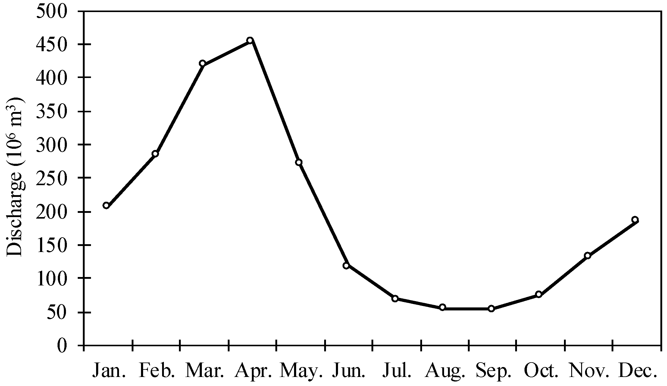
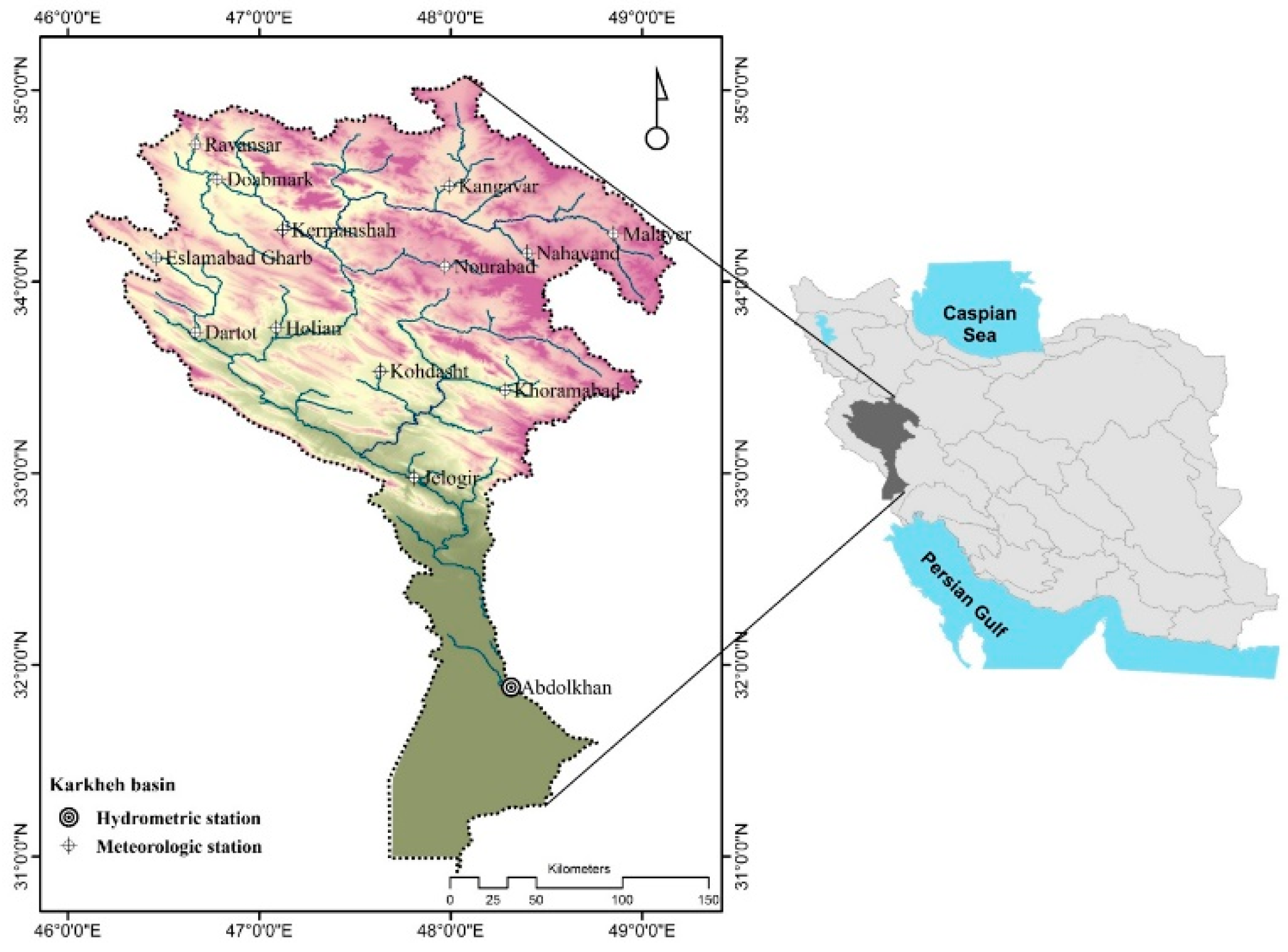
2.1. Case Study

The Karkheh basin covers 50,000 square kilometers in southwest Iran, at 30°58′ to 34°56′ N latitude and 46°06′ to 49°10′ E longitude. The Karkheh River is the main drainage of this catchment, which is composed of two main branches: Semireh and Kashkan. The output of this basin is measured at the Abdolkhan hydrometric station in the south of the watershed. Figure 1 depicts the distribution of monthly discharge at this station. In this research, discharge was simulated in monthly time steps for a period of 34 years (1967–2000) at the Abdolkhan station. It should be noted that after 2000, some water resource projects were developed in the basin, which significantly reduced river discharge downstream of the basin. So, due to the fact that the runoff was strongly affected by the anthropogenic alteration after 2000, we used the data collected prior to the year 2000. Fourteen rain-gauge stations throughout the Karkheh basin (Figure 2) were used to conduct R-R modeling. The specifications of these stations are given in

Table 1. Rain-gauge specifications in the Karkheh basin.

Station Name	Latitude	Longitude	Average (mm)	Max. (mm)	Min. (mm)	SD † (mm)
Doabmark	46°47′	34°34′	488	777	210	133
Dartot	46°39′	33°33′	443	623	232	103
Holian	47°46′	33°46′	336	613	100	118
Jelogir	46°47′	32°58′	470	793	259	151
Nourabad	47°48′	34°05′	461	833	152	133
Ravansar	46°40′	34°43′	548	773	334	96
Kangavar	48°00′	34°30′	395	620	222	84
Kermanshah	47°07′	34°16′	475	859	259	124
Malayer	48°18′	34°15′	305	413	132	55
Nahavand	48°24′	34°09′	396	593	226	87
Eslamabad Gharb	46°48′	34°07′	500	699	258	88
Kohdasht	47°38′	33°32′	444	631	246	87
Khoramabad	48°17′	48°26′	520	806	275	134
Abdolkhan	48°22′	31°49′	229	434	92	78

^† Standard deviation.

. The Ravansar station had the maximum mean annual precipitation, at 548 mm, and Bostan had the lowest, at 208 mm. It should be mentioned that all the average values are climatological averages over the study period.

2.2. Databases

The CRU, GPCC, and APHRODITE precipitation data were used to implement R-R modeling in addition to the in situ information from 14 rain gauge stations and output discharge data during 1967–2000. From the 34 years of information, 14 data years were used for model training, 6 years for validation, and 14 for model testing.

2.2.1. APHRODITE

The APHRODITE project was started by the Research Institute for Humanity and Nature (RIHN) and the Meteorological Research Institute of Japan Meteorological Agency (MRI/JMA) in 2006. This database provides daily precipitation with 0.25° × 0.25° and 0.5° × 0.5° spatial resolutions. APHRODITE precipitation data are available from 1951 to 2007 for the Middle East. This study utilized the APHRODITE Middle East precipitation dataset V1101R1 at a 0.5° resolution for R-R modeling [59]. Precipitation data are available at http://www.chikyu.ac.jp/precip/ (accessed on 10 February 2024). It is worth mentioning that the temporal resolutions of the R-R modeling and APHRODITE precipitation are monthly and daily, respectively. Accordingly, the temporal resolutions of the APHRODITE data were converted to monthly values.

2.2.2. GPCC

The GPCC precipitation database was established in 1989 at the request of the World Meteorological Organization (WMO) and is managed by Deutscher Wetterdienst (DWD), Germany’s national meteorological agency. Monthly precipitation data are provided for users at 0.5° × 0.5°, 1° × 1°, and 2.5° × 2.5° spatial grid resolutions. This database offers a variety of rainfall data. In this study, reanalysis data (version 7) with a 0.5° × 0.5° resolution were used [60]. GPCC precipitation data were established from 75,000 ground rain gauges and are available from 1901 to 2013. These data are downloadable from http://www.esrl.noaa.gov/psd/data/gridded/data.gpcc.html (accessed on 10 February 2024).

2.2.3. CRU TS

CRU was founded at East Anglia University in England in 1972. This database provides various climatic information with different spatial resolutions for regions around the world. In this study, CRU TS 4.01 precipitation data were used [61]. These data are available for all parts of the world at a 0.5° × 0.5° spatial resolution and at a monthly temporal resolution from 1901 to 2016. CRU datasets are accessible from https://crudata.uea.ac.uk/cru/data/hrg/ (accessed on 10 February 2024).

2.3. Rainfall-Runoff Modeling

R-R modeling can be conducted with both data-driven and conceptual models. Using conceptual models requires a large amount of input information, and this is rarely suitable for developing countries. Therefore, in this study, the Multilayer Perceptron Neural Network (MLPNN), a data-driven model that many studies have proved effective (e.g., refs. [62,63]), was employed. The MLPNN with three layers can be a universal approximator [64]. The choice of the MLPNN as the rainfall-runoff (R-R) model in this study, particularly for handling incomplete discharge data, is grounded in its capability to approximate complex functions and adapt to diverse datasets. MLPNNs are distinguished by their ability to learn from input data and adapt to new, unseen data. This is especially beneficial in regions where the application of conceptual models is hindered by the scarcity of detailed input information. The inherent adaptability of MLPNNs renders them universal approximators, capable of modeling intricate relationships between inputs and outputs as commonly encountered in hydrological systems. However, the effectiveness of MLPNNs in such applications extends beyond their learning and adaptability traits. These models undergo a rigorous process that encompasses training, where the model learns the underlying patterns from a subset of the data; calibration, which involves adjusting the model parameters to align predictions closely with real-world observations; and testing, a critical phase where the model’s performance is evaluated on a separate dataset not used during the training. This testing phase is essential for assessing the model’s generalization capability, ensuring it can accurately predict outcomes in varied and unseen scenarios. Together, these steps ensure that MLPNNs can be effectively applied in R-R modeling, offering reliable predictions even in the face of incomplete discharge data and complex hydrological dynamics. The MLPNN was trained using a supervised learning algorithm based on the LM algorithm. The learning process was designed to minimize the following function [65]:

$$E=\frac{1}{L}{\displaystyle \sum _{l=1}^L(y_l-{\widehat{y}}_l}{)}^2$$

(1)

where L is the number of data, y_l is the lth observational output, and is the lth forecasted output. To calculate the $\widehat{y}$ in a three-layer network with m neurons in the hidden layer and n independent variables (number of inputs), Equation (2) was used:

$$\widehat{y}=f\left[{\displaystyle \sum _{j=1}^m{w}_j.g({\displaystyle \sum _{i=1}^n{w}_{ji}{x}_i+b_{j0})+b_o}}\right]$$

(2)

where w_j is the weight that connects the jth neuron in the hidden layer and the neuron of output layer, wji is the weight related to the relation between the ith input variable and jth neuron in the hidden layer, x_i is the ith independent variable, b_j0 is the bias of the jth neuron of hidden layer, b₀ is the bias related to the output neuron, g is the activation function for neuron of hidden layer, and f is the activation function for the output layer.

LM is a fast and powerful algorithm, but it is possible to become stuck in the local optimum in this approach [66,67]. Thus, many researchers have employed evolutionary algorithms (EAs) as an alternative to the LM algorithm (e.g., refs. [68,69]). Although EAs are safe from becoming stuck in the local optimum, they are prone to overfitting due to considering each item in the training information singly. For this reason, some researchers have employed an objective function of optimization algorithms as a weighted combination for training and validating neural network data (e.g., ref. [70]). However, determining the appropriate weights for training and validation is another challenge. In this study, the NSGA-II was used to train the ANN precisely and appropriately. The NSGA-II can consider training and validation data at the same time to determine the weights and biases of the neural network. As such, the resulting network will be safe from overfitting while being trapped in the local optimum.

In this study, two scenarios were considered for R-R modeling. In the first scenario, R-R modeling was calibrated based on in situ data, and gridded precipitation datasets were used in the testing phase. The distribution of the 14 rain gauge stations, which are predominantly located in high and mid–high elevations within the Karkheh basin, inherently aids in delineating the heterogeneity of precipitation areal distribution in these elevational bands. In the second phase, model calibration and testing were performed separately for each dataset. Before entering information into the MLPNN, PCA and SVD were performed as pre-processing measures to reduce the size of the data. Figure 3 shows a flowchart of the different R-R models. Altogether, eight models were developed, which are marked with colored rectangles. Therefore, eight different time series of discharge were simulated.

2.4. Non-Dominated Sorting Genetic Algorithm II (NSGA-II)

The NSGA-II is an evolutionary optimization algorithm that is used in multi-objective problems. This algorithm starts by generating a set of random solutions; the objective function value is then calculated for each solution, and the process of refining the solutions begins. At this step, the solutions are selected for crossover using the binary tournament operator based on two criteria: non-dominated sorting and crowding distance. The algorithm can be kept from becoming stuck in the local optimum by applying a mutation operator. The objective function values are calculated once again after the refining solutions are determined. This process is repeated until one of the stopping criteria is satisfied. In each generation, non-dominated solutions in objective space constitute a pareto front; any point on this front can be an optimal solution of the problem. (More information about the NSGA-II is available in [71]). In this research, the mean squared error (MSE) of the training and validation of the MLPNN were considered as two objective functions to determine the optimum values of the neural network weights and biases as follows:

$$Minimize =\left\{\begin{array}{l}MS{E}_{train}: f_1(w,b)=\frac{1}{C}{\displaystyle \sum _{c=1}^C{(f{\left[{\displaystyle \sum _{j=1}^m{w}_j.g({\displaystyle \sum _{i=1}^n{w}_{ji}{x}_i+b_{j0})+b_o}}\right]}_c-y_c)}^2}\\ MS{E}_{validation}: f_2(w,b)=\frac{1}{D}{\displaystyle \sum _{d=1}^D{(f{\left[{\displaystyle \sum _{j=1}^m{w}_j.g({\displaystyle \sum _{i=1}^n{w}_{ji}{x}_i+b_{j0})+b_o}}\right]}_d-y_d)}^2}\end{array}\right.$$

(3)

where w and b are the weight and bias of the neural network (decision variables of optimization problem), and C and D are the number of training and validation data points, respectively.

2.5. Data Pre-Processing

Since precipitation data from 14 stations were considered as the model input and a two-step delay was applied for the precipitation data, there were a total of 42 inputs into the R-R model, making it time consuming to run. Therefore, PCA and SVD were employed to reduce the data dimensions. Hence, three principal components (PCs) of these approaches were used as the model input to explain over 80% of the data variance. Since the rest of the PCs did not add significant information (all 39 components came to less than 20%), we only selected three PCs. These two methods are described below.

2.5.1. Principal Component Analysis

PCA is a data pre-processing method that aims to reduce the dimension of the problem. By using PCA, large numbers of correlated variables can be replaced with a limited number of new linearly uncorrelated variables called principal components (PCs). In mathematical terms, PCA is an orthogonal linear transformation that rotates the coordinate system so that the largest data variance is placed on the first coordinate axis, the second largest variance on the second axis, etc. Therefore, it can preserve initial information with a lower number of variables and finer accuracy. If the equation is a random vector with a certain non-negative covariance matrix and are eigenvalues of $\sum$. a₁, a₂, …, a_H are corresponding eigenvectors of ${\lambda }_1,{\lambda }_2,\dots ,{\lambda }_H$. Defined PC₁, PC₂, …, PC_H variables called PC listed below:

$$\begin{array}{l}P{C}_1=a_{11}{X}_1+a_{21}{X}_2+\dots +a_{H1}{X}_H\\ P{C}_2=a_{12}{X}_1+a_{22}{X}_2+\dots +a_{H2}{X}_H\\ \begin{array}{c}P{C}_3=a_{13}{X}_1+a_{23}{X}_2+\dots +a_{H3}{X}_H\\ ⋮\\ P{C}_H=a_{1H}{X}_1+a_{2H}{X}_2+\dots +a_{HH}{X}_H\end{array}\end{array}$$

(4)

PCH is called the Hth principal component. PCs are calculated in a way that PC₁ justifies the maxi-mum variance and PC₂ possesses the maximum variance that was not considered by PC₁; this process continues until the last component is reached.

2.5.2. Singular Value Decomposition

SVD considers not only the dependent variables but the independent ones as well in determining significant components. Therefore, SVD has to be applied on a covariance matrix obtained from multiplying independent variables by dependent variables. The SVD procedure converts the rectangular matrix into three matrices: orthogonal (U), diagonal (S), and transpose of an orthogonal matrix (V), which can be expressed mathematically as follows [72]:

$$A_{ke}=U_{kk}{S}_{ke}{V}_{ee}^T$$

(5)

where U and V are orthogonal matrices, U^TU = I and V^TV = I, and S is a pseudo-diagonal matrix with zero values as its entries. The columns of U and V are orthonormal eigenvectors of AA^T and A^TA, respectively [2]. In this study, SVD was applied to an R-R covariance matrix. For this purpose, the following covariance matrix was used:

$$Co{v}_{P\&Q}=\frac{1}{nm}\times \left(\begin{array}{l}{P}_{1,1} \cdots P_{1,nm}\\ ⋮ \ddots ⋮\\ P_{s,1} \cdots P_{s,nm}\end{array}\right)\times \left(\begin{array}{l}{Q}_1\\ ⋮\\ Q_{nm}\end{array}\right)$$

(6)

where $Co{v}_{P\&Q}$ is the R-R covariance matrix, nm is the number of months of study, P is the precipitation, and Q is the discharge. The main component of precipitation was calculated as follows:

$$P(z)=\left(\begin{array}{l}{P}_{1,1} \cdots P_{1,nm}\\ ⋮ \ddots ⋮\\ P_{s,1} \cdots P_{s,nm}\end{array}\right)\times U(:,z)$$

(7)

where z ranges from one to the number of significant modes in the maximum situation [73]. It should be mentioned that the above operation is performed on a set of calibration data and after the extraction of matrix U, the matrix can be used to test the model. It is possible to update matrix U by adding new discharge data gradually.

2.6. Evaluation Criteria

Three efficiency criteria were considered for judging the performance of precipitation databases and different models. The first criterion was correlation coefficients (CCs) with values between −1 and 1, where a value close to 1 represents direct correlation between two compared time series. The second criterion was root mean square error (RMSE), which is calculated from investigated data; its values range from 0 to positive infinity, with lower values indicating better performance. The last criterion is Bias, which is expressed as a percentage and represents the ratio of the model outputs to real values. Equations of these criteria are listed below [74,75]:

$$CC=\frac{{\displaystyle \sum _{l=1}^L(y_l-\overline{y})({\widehat{y}}_l-\overline{\widehat{y}})}}{\sqrt{{\displaystyle \sum _{l=1}^L{(y_l-\overline{y})}^2{\displaystyle \sum _{l=1}^L{({\widehat{y}}_l-\overline{\widehat{y}})}^2}}}}$$

(8)

$$RMSE=\sqrt{\frac{{\displaystyle \sum _{l=1}^L{(y_l-{\widehat{y}}_l)}^2}}{L}}$$

(9)

$$Bias=\frac{{\displaystyle \sum _{l=1}^L{\widehat{y}}_l-{\displaystyle \sum _{l=1}^L{y}_l}}}{{\displaystyle \sum _{l=1}^L{y}_i}}\times 100$$

(10)

In the above equations, y and $\widehat{y}$ are the observational data and the output data from the model, respectively.

3. Results and Discussion

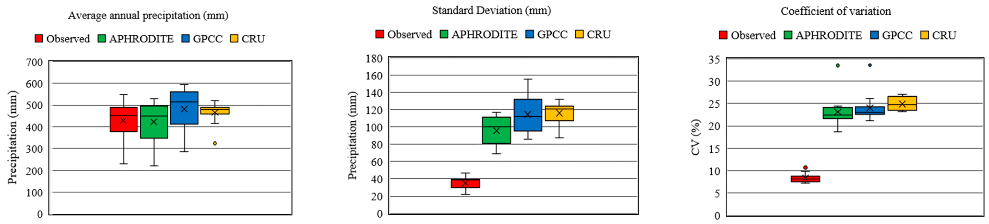
3.1. Evaluation of Precipitation Data

Although the main purpose of this study is to evaluate dataset information for R-R simulations, the performance of the model depends on the accuracy of the data input into the R-R model. Therefore, this section describes the brief assessment of the precipitation dataset. Figure 4 shows the observational precipitation regime alongside the precipitation regime from the datasets in the Karkheh basin. The APHRODITE data are closely aligned with the observational data. The GPCC data overestimate the observational precipitation by 19, 28, and 28 percent in January, March, and April, respectively. The CRU data overestimate the precipitation amount in most months; the biggest difference is in April, with a difference of 14 mm. These comparisons show that the datasets have distinguished the regimes of precipitation properly but possess bias in most months.

Table 2. Comparison criteria of precipitation datasets with observed precipitation.

Dataset	Annual Time Series			Monthly Time Series †
	Mean (mm)	SD (mm)	CV (%)	CC	RMSE (mm)	Bias (%)
Observed	429.17	76.63	17.86
APHRODITE	422.66	84.42	19.97	0.81	22.13	−1.52
GPCC	482.64	97.08	20.12	0.80	26.23	11.08
CRU	466.80	107.58	23.05	0.78	24.23	8.77

^† Compared with the observed precipitation.

shows each dataset’s statistical indicators and evaluation criteria in comparison with the observational data. On an annual scale, the APHRODITE data are close to the observational data, estimating annual mean precipitation with a 6.5 mm (−1.5%) disagreement. Other statistical properties, such as the standard deviation (SD) and coefficient of variation (CV), were close to the observational data as well. In terms of statistical indicators, the CRU data performed, on average, better than the GPCC data. These two databases overestimated the mean precipitation by approximately 44 and 53 mm, respectively, but GPCC performed better in terms of SD and CV. SD values from GPCC and CRU differed from the observational data by 21% and 29%, and the CV values varied by 2% and 5%, respectively. According to the efficiency criteria, CRU displayed better RMSE and Bias than GPCC, but GPCC gave a more satisfactory CC. Thus, in this basin, the APHRODITE dataset showed the best performance in terms of the efficiency criteria and statistical indicators for mean annual precipitation. The CRU and GPCC datasets performed almost identically; the minor differences between them can be seen in Table 2.

Average annual rainfall was examined based on a box-plot of the 14 investigated stations. According to Figure 5, APHRODITE was close to the observed values in terms of precipitation variation in the investigated stations; GPCC gave results higher than the observed data by almost the same amount. Meanwhile, the CRU chart included more differences than the other two, and out of range data were observed in this database. Although the databases have almost similar behaviors in respect of their standard deviations and coefficients of variation, all the databases are diverse from the observed data. The mean annual rainfall standard deviation in the 14 observational stations is 35 mm, and for APHRODITE, GPCC, and CRU it is 96, 114, and 116 mm, respectively. Likewise, the APHRODITE, GPCC, and CRU means of annual rainfall coefficients of variation are different from observed values by 15, 16, and 17 percent, respectively.

Because the output discharge simulation was based on the monthly scale in the Karkheh basin, this study assessed each dataset’s performance for each month separately. As shown in

Table 3. Monthly comparison criteria of precipitation datasets with observed precipitation.

Dataset		Mean (mm)	SD (mm)	CV (%)	CC	RMSE (mm)	Bias (%)		Mean (mm)	SD (mm)	CV (%)	CC	RMSE (mm)	Bias (%)
Observed	Jan.	63.83	15.62	24.47				Jul.	0.16	0.44	273.98
APHRODITE		65.06	26.51	40.75	0.79	16.87	1.92		0.82	1.55	187.96	0.79	1.38	416.15
GPCC		75.68	31.59	41.75	0.79	24.24	18.56		1.14	1.51	131.63	0.74	1.55	617.51
CRU		64.10	28.72	44.81	0.83	17.85	0.43		3.82	7.62	199.14	0.32	8.24	2299.73
Observed	Feb.	69.35	17.31	24.95				Aug.	0.06	0.11	189.66
APHRODITE		61.67	22.65	36.72	0.67	18.36	−11.07		0.36	0.68	190.58	0.26	0.72	493.77
GPCC		68.35	25.52	37.34	0.67	18.71	−1.44		0.52	1.00	191.43	0.33	1.06	764.65
CRU		59.99	26.42	44.05	0.74	19.94	−13.50		4.32	8.87	205.46	0.24	9.69	7064.96
Observed	Mar.	69.83	20.93	29.97				Sep.	5.50	4.33	78.76
APHRODITE		78.76	35.44	45.00	0.76	25.06	12.80		0.73	1.14	155.50	0.24	6.31	−86.64
GPCC		89.10	39.38	44.20	0.75	33.19	27.59		1.25	2.87	228.76	0.04	6.58	−77.19
CRU		82.51	37.08	44.94	0.78	27.18	18.16		2.74	5.54	202.20	0.30	6.44	−50.16
Observed	Apr.	49.23	19.45	39.50				Oct.	26.75	17.14	64.09
APHRODITE		54.75	29.11	53.17	0.88	15.86	11.23		20.04	22.99	114.70	−0.01	29.17	−25.06
GPCC		62.77	32.80	52.25	0.89	22.21	27.50		20.16	25.09	124.46	−0.01	30.78	−24.62
CRU		63.43	36.63	57.75	0.88	25.54	28.85		23.24	27.67	119.06	−0.01	32.44	−13.11
Observed	May.	25.40	17.31	68.12				Nov.	52.20	22.12	42.38
APHRODITE		25.90	19.79	76.40	0.80	11.77	1.95		51.49	44.71	86.83	0.06	47.89	−1.36
GPCC		27.24	22.73	83.46	0.75	14.82	7.21		62.64	51.32	81.92	0.05	55.05	20.00
CRU		36.52	28.98	79.35	0.80	21.33	43.76		51.06	40.13	78.60	−0.02	45.59	−2.19
Observed	Jun.	3.12	2.78	89.03				Dec.	63.74	15.31	24.02
APHRODITE		1.46	2.12	145.34	0.49	3.00	−53.21		61.61	29.85	48.45	0.06	32.28	−3.35
GPCC		2.13	3.03	142.65	0.52	2.98	−31.88		71.68	36.12	50.39	0.08	38.36	12.45
CRU		7.41	10.58	142.77	0.42	10.52	137.45		67.66	29.69	43.87	0.07	32.20	6.15

, in most cases, the statistical indicators and evaluation criteria were favorable for the datasets in months with higher amounts of rainfall. In contrast, they did not provide acceptable evaluation criteria values in low-rainfall months. In practical hydrological applications, the accuracy of these criteria reveals significant limitations. For instance, during August, the observed correlation between rainfall data and the values from the GPCC, APHRODITE, and CRU datasets was recorded to be 0.26, 0.33, and 0.24, respectively. Additionally, the Bias percentages for these datasets were notably high, with figures standing at 494%, 765%, and 7065%, indicating a substantial deviation from the observed values. These results illustrate an underperformance of the datasets, whereas the difference between the observed precipitation data and the three gridded datasets are only 0.30, 0.46, and 4.25 mm, respectively. Therefore, relying only on statistical indicators can lead to a better evaluation of the results, which are better during dry months, i.e., June to September. The best performances among the datasets are shown in Table 3 in terms of evaluation criteria and statistical indicators. Overall, APHRODITE fulfilled the objectives better than the two other databases.

3.2. Rainfall-Runoff Modeling

After assessing dataset precipitation, R-R modeling was implemented using the investigated datasets. As mentioned before, two scenarios, two pre-processing methods, and two training algorithms for the MLPNN were considered to conduct the R-R modeling. One of the key elements affecting the performance of the MLPNN was the number of hidden-layer neurons, which were calculated by trial and error. With each number of neurons in the range of 5 to 20, five runs were carried out from the MLPNN, and the average model performance was used as a benchmark to determine the appropriate number of neurons. After determining the optimal number of neurons, the MLPNN was run 50 times based on the LM training algorithms (under different scenarios and pre-processing methods); the best MLPNN performance was determined to be MLPNN-LM. The MLPNN training was also conducted using the NSGA-II. After optimizing the biases and weights of the various MLPNNs (under different scenarios and pre-processing methods), the NSGA-II algorithm was considered with 5000 generations and a population of 500 based on uniform mutation and a two-point crossover operator at the rates of 0.03–0.10 and 0.6–0.8, respectively. The ideal point from pareto was chosen such that the sum of the MSE distance of the training and validation values from the ideal value (which is equal to zero) became the minimum. In other words, a point in the pareto front was considered as the solution such that $\sqrt[ ]{MS{E}_{train}^2+MS{E}_{Validation}^2}$ was minimal; the weights and biases of the MLPNN were determined based on this solution.

Table 4. Criteria for evaluating the comparison between observed and simulated discharge using datasets and various methodologies. Cells highlighted in yellow indicate the best performance according to each criterion.

	Dataset	Pre-Processing	Training Algorithm	Train			Validation			Test			PCA	SVD	LM	NSGA-II	PCA	SVD	PCA	SVD
				CC	RMSE	Bias	CC	RMSE	Bias	CC	RMSE	Bias					LM	LM	NSGA-II	NSGA-II
Scenario 1	Observed	PCA	LM	0.90	90.73	2.73	0.86	65.21	−5.03	0.82	104.03	−3.44	6		4	2	4		2
		PCA	NSGA-II	0.90	88.02	−1.68	0.83	72.38	−7.25	0.80	110.27	−1.40
		SVD	LM	0.90	89.77	5.20	0.84	70.47	−4.96	0.81	104.10	−5.44		7	2	5		2		5
		SVD	NSGA-II	0.90	89.52	1.24	0.82	71.02	−10.09	0.82	100.07	0.29
	APHRODITE	PCA	LM							0.67	153.54	−4.93	0		0	0	0		0
		PCA	NSGA-II							0.65	166.40	−2.87
		SVD	LM							0.64	173.57	12.15		3	0	3		0		3
		SVD	NSGA-II							0.68	137.33	2.38
	GPCC	PCA	LM							0.66	166.60	−0.58	1		1	0	1		0
		PCA	NSGA-II							0.65	179.90	5.16
		SVD	LM							0.64	193.70	22.16		2	0	2		0		2
		SVD	NSGA-II							0.67	148.82	7.19
	CRU	PCA	LM							0.63	152.64	−13.60	1		1	0	1		0
		PCA	NSGA-II							0.61	165.95	−9.71
		SVD	LM							0.60	167.72	5.38		2	0	2		0		2
		SVD	NSGA-II							0.61	149.20	−1.32
Scenario 2	APHRODITE	PCA	LM	0.89	90.84	−4.49	0.78	85.45	−6.95	0.71	136.66	−0.15	7		3	4	3		4
		PCA	NSGA-II	0.90	89.59	−0.03	0.77	92.50	0.76	0.72	124.59	1.29
		SVD	LM	0.88	95.16	−2.17	0.77	83.57	−0.90	0.73	126.82	1.20		3	1	2		1		2
		SVD	NSGA-II	0.89	92.07	1.00	0.72	92.00	1.45	0.74	124.53	7.03
	GPCC	PCA	LM	0.90	86.83	2.13	0.76	87.84	−5.09	0.71	139.34	2.54	3		1	2	1		2
		PCA	NSGA-II	0.92	81.51	2.25	0.75	94.08	−1.69	0.72	125.74	−2.41
		SVD	LM	0.90	88.96	0.14	0.76	83.32	3.09	0.71	124.63	1.77		8	3	5		3		5
		SVD	NSGA-II	0.92	80.18	1.43	0.77	84.71	−2.31	0.72	129.44	−1.36
	CRU	PCA	LM	0.84	108.59	1.04	0.71	92.95	1.48	0.69	128.30	−6.30	2		1	1	1		1
		PCA	NSGA-II	0.85	107.43	−2.74	0.72	93.98	−4.00	0.71	125.88	−8.52
		SVD	LM	0.86	104.71	−1.28	0.72	92.10	−2.01	0.72	124.60	−7.49		8	3	5		3		5
		SVD	NSGA-II	0.87	99.97	−2.73	0.70	93.91	−0.41	0.71	124.56	−0.73
												SUM	20	33	20	33	11	9	9	24

gives the results of the R-R modeling under different conditions. In total, 16 different models were trained; 4 models related to the first scenario and 12 models to the second scenario. The contributions of each pre-processing method (PCA and SVD) and training algorithm (LM and the NSGA-II) were used to train six models. The results indicated that all three precipitation databases in the second scenario performed better than in the first scenario. This superiority was more evident in the case of GPCC and CRU. According to the reviewed results in the assessment of precipitation, it was expected that APHRODITE would perform better than GPCC and CRU in the first scenario due to the proximity of this dataset information to the observed data. In the second scenario, the various databases showed some disagreement with the observed precipitation. These differences, which often appear in Bias, may be troublesome in meteorology studies and need to be corrected; however, in R-R modeling using the MLPNN, Bias can be automatically corrected by establishing the relation between runoff and rainfall. This could be the reason for the better performance in the second scenario compared to the first one. Therefore, the use of datasets in the calibration phase is recommended. Additionally, it should be mentioned that a period was chosen for calibration in which no major anthropogenic changes took place. This selection was critical to ensuring the integrity of the model calibration, allowing for a more accurate representation of the natural rainfall-runoff processes devoid of significant human-induced alterations.

In Table 4, the column headed “superiority count” represents the summation of the superiority times of a pre-processing method (PCA or SVD), a training algorithm (LM or the NSGA-II), or a combination of them based on the three evaluation criteria of CC, RMSE, and Bias. Although in some cases the differences are very minor, in order to provide a quantitative criterion for assessing the models, the criteria were compared up to two decimal digits’ precision. In Table 4, the green cells show the best values for efficiency criteria in R-R modeling using the different datasets. For instance, in all cases the CC is equal to 0.90 based on the observed data in the training phase of the first scenarios, so all of them are marked in green. The RMSE of the first-scenario training phase has a minimum value of (88.02 × 10⁶ m³) using PCA pre-processing and the NSGA-II (S1-PCA-NSGA-II); thus, this value is highlighted in green as well. Accordingly, in comparing pre-processing methods, PCA and SVD performed 20- and 33-times better (considering all different scenarios), respectively. Therefore, it can be concluded that the SVD operation is superior to PCA in data pre-processing. In assessing the algorithms training, the NSGA-II had the best performance at 33-times better than the LM algorithm, compared to 20-times better for the LM algorithm. Combining SVD and the NSGA-II, with a superiority count of 24, yielded the highest number of advantages, followed by the combination of PCA and LM, which performed 11 times better and stands in the second rank.

Based on the results presented in Table 4, in most cases, the RMSE of the LM algorithm in the validation phase gave better results than the NSGA-II because the LM algorithm determines the best weights and biases of the MLPNN based on the MSE of validation. Since this optimization algorithm is mono-purpose, it cannot consider both training and validation together. Although the NSGA-II was slightly weaker than LM in RMSE, which was related to validation, it gave a better balance between validation and training. Overall, in these two aspects of the efficiency criteria it performed better than LM. Although it is possible to choose points with primary attention to validation or training data in the pareto front, the best situation is one in which a point is considered as the balance that satisfies both aspects. In this study, the point with the lowest value of $\sqrt[ ]{MS{E}_{train}^2+MS{E}_{Validation}^2}$ was considered to be ideal. According to the results, all the datasets performed better in the second scenario than in the first. In this regard, the APHRODITE database based on the S2-PCA-NSGA-II model, and also GPCC and CRU databases based on S2-SVD-NSGA-II for a total of three training steps, validation, and testing, gave the best results. R-R simulation with the observed precipitation data worked the best based on SVD-NSGA-II as well.

The distributions of the observed and simulated discharge related to the testing aspects of the various mentioned models are shown in Figure 6. Low-flow values were more accurately estimated than high-flow values. In the analysis of the first scenario within Figure 6, it is noted that there is a larger number of points above the line y = x compared to the second scenario. This observation is critical as it suggests an overestimation of runoff in the first scenario. The line y = x serves as a benchmark for perfect model performance, where the observed and simulated discharges match exactly. Therefore, points above this line indicate instances where the model predicted more runoff than was actually observed, highlighting potential areas for model adjustment or reevaluation. Conversely, the second scenario demonstrates a more balanced approach to runoff simulation, as evidenced by a more even distribution of points on both sides of the line y = x. This balance suggests that the models used in the second scenario provide a more accurate representation of runoff, possibly due to the utilization of various datasets that enhance model precision. Notably, the models S1-SVD-LM and S2-SVD-LM, when employing GPCC data, exhibited significant improvements in performance. This improvement indicates the value of selecting appropriate datasets for enhancing model accuracy, especially in complex hydrological simulations. Figure 7 represents the empirical cumulative distribution function (eCDf) of the observational discharge data alongside the simulated discharge according to the best results of each dataset for each month. This chart was drawn based on the calibration and testing data. The months with a high rate of discharge demonstrated proper functioning for the datasets as a whole. These performances are acceptable in the first five months and last month of year, which are of the greatest hydrological importance for the Karkheh basin. However, inconsistencies were present in the months with low discharge rates; the most significant conflict can be observed from June to September. Comparing the simulated discharge using dataset precipitation with that using observational precipitation data may be fairer rather than comparing it to the observed discharge. In this regard, few months can be found in Figure 7 in which the observed precipitation information has significant superiority to the results using the datasets in the discharge simulation. None of the datasets are absolutely paramount over entire months.

4. Conclusions

(1)

This study attempted to find an operational approach to simulate discharge or fill in the gaps that existed in discharge data over a poorly gauged basin. To this end, three gridded precipitation datasets (APHRODITE, GPCC, and CRU) were evaluated = on their accuracy in depicting hydrological behavior in the Karkheh basin in Iran during 1967–2000. The results can be presented in two parts.

(2)

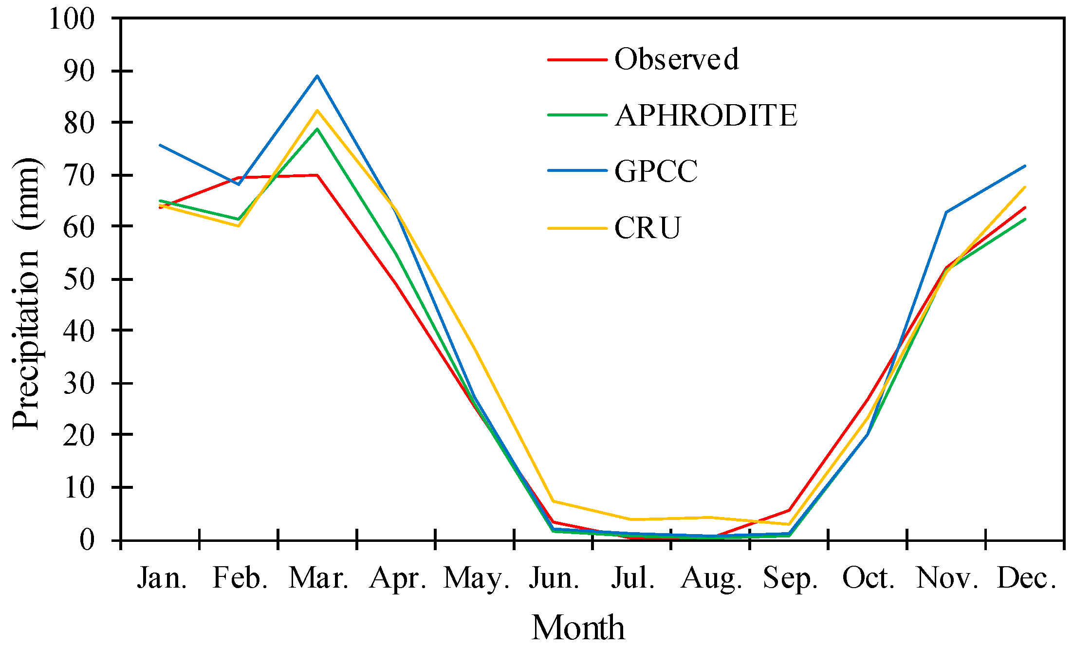
The first one is the comparison between in situ precipitation and girded datasets, and the second part is the assessment of R-R modeling results. The comparison of the precipitation datasets showed that APHRODITE outperformed the other datasets. For instance, on an annual scale, the average difference between APHRODITE precipitation and in situ data is 6.5 mm, while the values of this difference for the GPCC and CRU data are approximately equal to 53 and 44 mm, respectively. The findings align closely with those reported in references [56] and [45]. The analysis reveals that although the datasets accurately identify different patterns in precipitation, they exhibit biases in most months, and they possess bias in the majority of months.

(3)

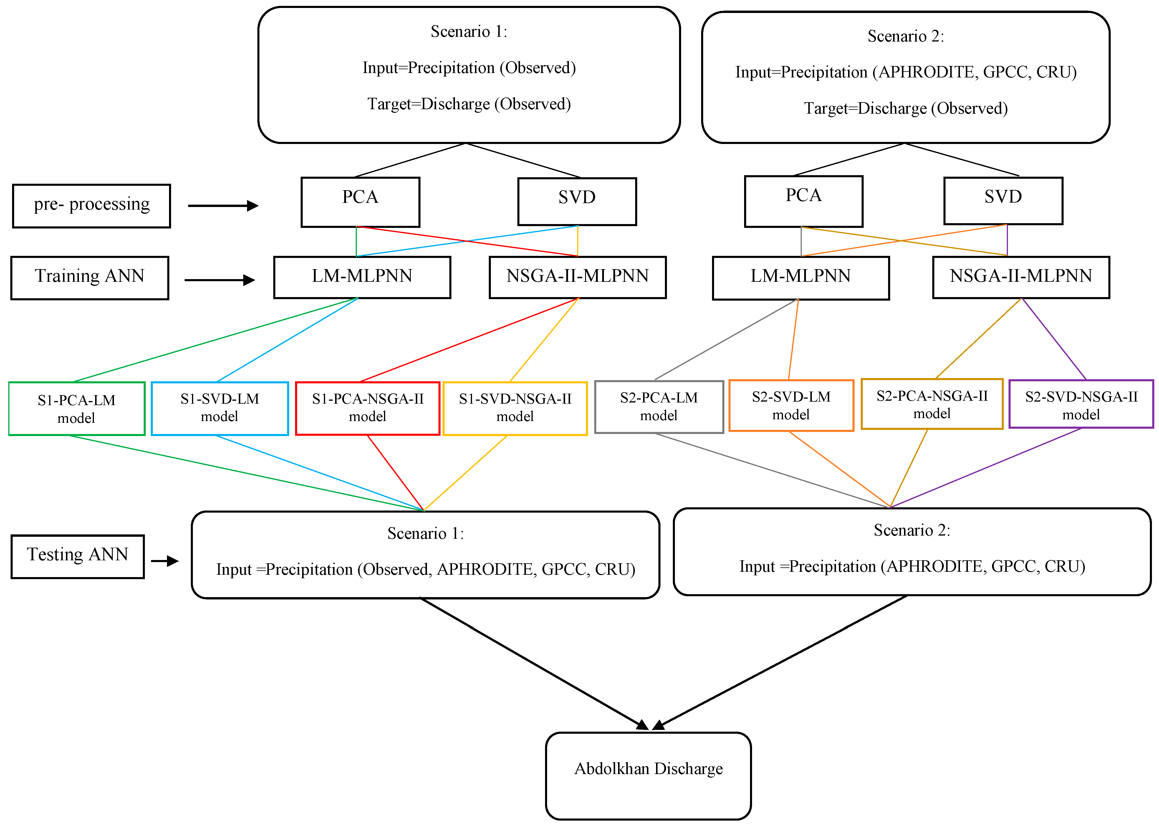
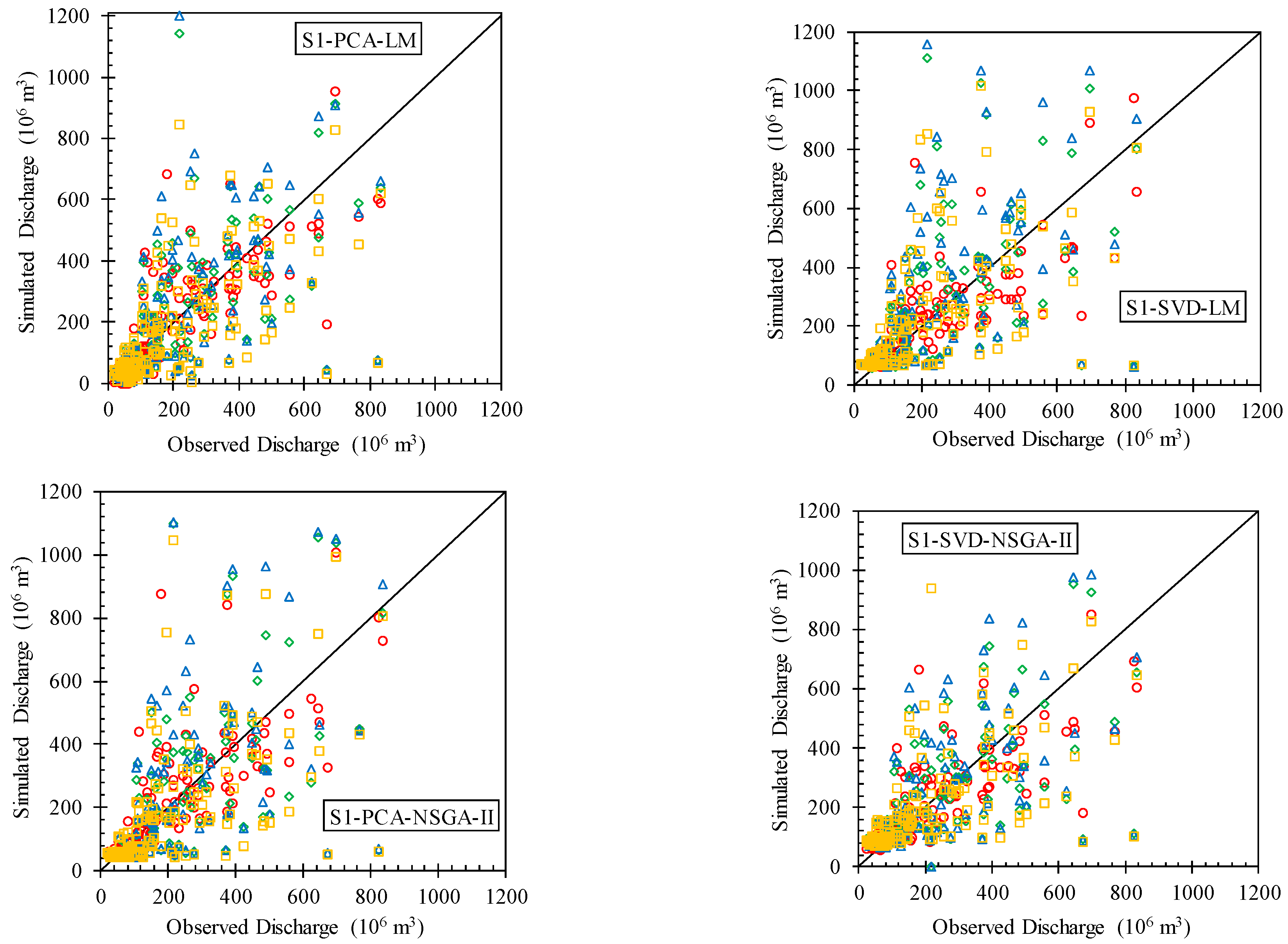
After comparing the precipitation data, the development of an R-R model was investigated to simulate the outflow of the Karkheh basin. The MLPNN was used in the R-R modeling. Due to the fact that the number of inputs of the R-R model was equal to 42, PCA and SVD were employed to reduce the dimensions of the datasets. In the next step, to train the model, with regard to being stuck in the local optimum of the LM algorithm, the NSGA-II was employed to determine network weights and biases, and its results were compared with LM. Two scenarios were chosen for model calibration: in the first scenario, the MLPNN was calibrated based on the observed precipitation, and it was examined based on observed and gridded precipitation; in the second scenario, the calibrating and testing of the model were performed separately for each dataset.

(4)

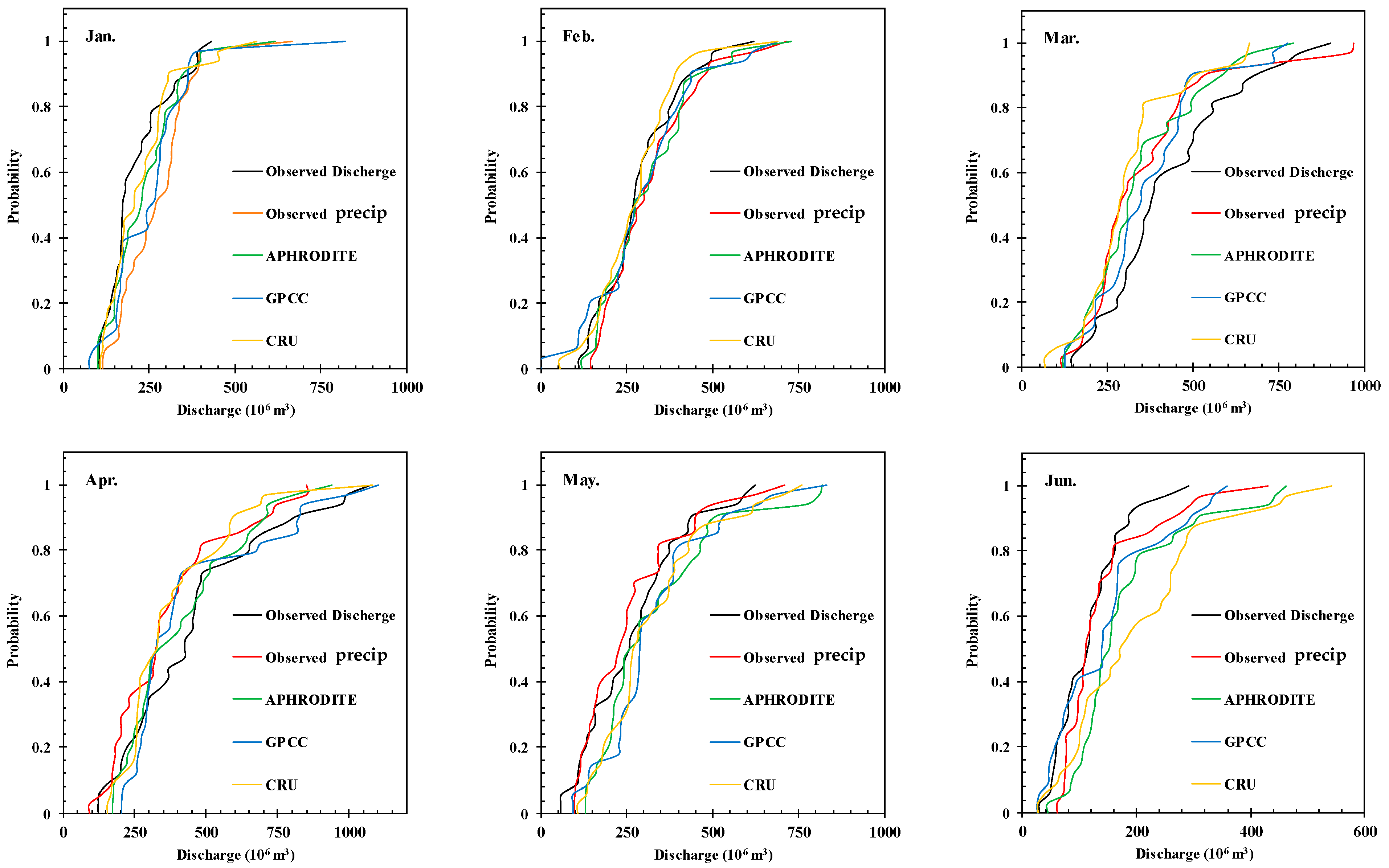
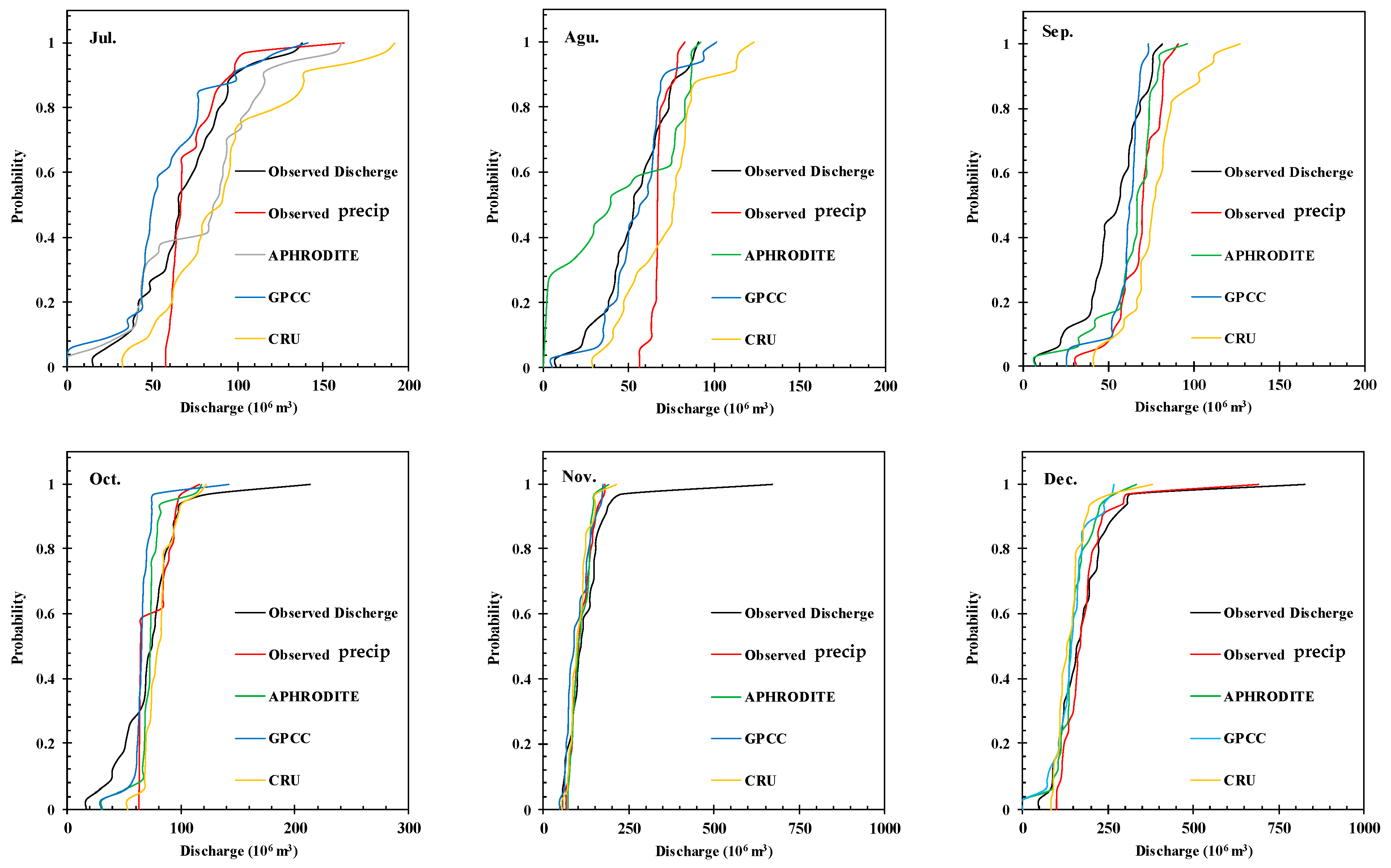
The R-R modeling results showed that the models were more efficient, and all three databases demonstrated appropriate performances in the second scenario. Because the main error in the gridded precipitation dataset is the bias error, it will disappear automatically when the model is calibrated using gridded precipitation datasets. The results were better for wet months than for dry months. Overall, the comparison between pre-processing methods indicated that SVD gave superior results to PCA. These results match well with the findings of [2]. Again, the NSGA-II operated better than LM in model training. To sum up, APHRODITE, based on the S2-PCA-NSGA-II model, and GPCC and CRU, based on the S2-SVD-NSGA-II model, had the best performances, and can be considered as alternatives for hydrological studies.

(5)

It should be indicated that the spatial resolution of APHRODITE is half that of the other two datasets, which can improve the accuracy of the modelling. Nevertheless, temporal resolutions of the datasets in this study are not important because all of the modeling process was performed at monthly scale. It is worth mentioning that GPCC and CRU have a reasonable lag time to updating their data while APHRODITE data are updated with a significant delay. This deficiency can be considered a weakness for APHRODITE data. So, before practical application, it is suggested that spatial–temporal resolution and the lag time of updating data should be considered in addition to the accuracy of the given datasets. Also, a combination of different datasets may improve R-R modeling performance. Hence, hybrid dataset development is suggested for future studies. Based on the results in poorly gauged basins, it is recommended that the same dataset be used to calibrate and test the model in order to perform R-R modeling. Thus, applying an existing model for discharge reconstruction or to fill the gap based on gridded precipitation may not achieve good accuracy. According to the results of this study, a well-trained ANN is very practical in hydrological applications and, therefore, the model’s calibration should be completed attentively. Future research should aim to overcome the limitations noted, particularly the variable performance of models in periods of low discharge rates. Recognizing these difficulties will steer further studies to enhance simulation precision in comparable hydrological scenarios, fostering a deeper insight into and utilization of discharge modeling methodologies. In conclusion, this study’s findings illuminate the path forward for hydrological modeling in data-scarce regions, advocating for a nuanced approach to dataset selection, model calibration, and optimization. By leveraging advanced computational techniques and a thorough understanding of dataset characteristics and limitations, researchers and practitioners can enhance the precision and reliability of hydrological models, thereby improving water resource management and planning outcomes in similar contexts worldwide.

References

1. ASCE Task Committee on Application of Artificial Neural Networks in Hydrology. Artificial Neural Networks in Hydrology. I: Preliminary Concepts. J. Hydrol. Eng. 2000, 5, 115–123. [Google Scholar] [CrossRef]
2. Chitsaz, N.; Azarnivand, A.; Araghinejad, S. Pre-processing of data-driven river flow forecasting models by singular value decomposition (SVD) technique. Hydrol. Sci. J. 2016, 61, 2164–2178. [Google Scholar] [CrossRef]
3. Yaseen, Z.M.; Fu, M.; Wang, C.; Mohtar, W.H.M.W.; Deo, R.C.; El-shafie, A. Application of the Hybrid Artificial Neural Network Coupled with Rolling Mechanism and Grey Model Algorithms for Streamflow Forecasting Over Multiple Time Horizons. Water Resour. Manag. 2018, 32, 1883–1899. [Google Scholar] [CrossRef]
4. Araghinejad, S.; Fayaz, N.; Hosseini-Moghari, S.-M. Development of a Hybrid Data Driven Model for Hydrological Estimation. Water Resour. Manag. 2018, 32, 3737–3750. [Google Scholar] [CrossRef]
5. Thakur, B.; Kalra, A.; Ahmad, S.; Lamb, K.W.; Lakshmi, V. Bringing statistical learning machines together for hydro-climatological predictions—Case study for Sacramento San joaquin River Basin, California. J. Hydrol. Reg. Stud. 2020, 27, 100651. [Google Scholar] [CrossRef]
6. Ghobadi, F.; Kang, D. Multi-Step Ahead Probabilistic Forecasting of Daily Streamflow Using Bayesian Deep Learning: A Multiple Case Study. Water 2022, 14, 3672. [Google Scholar] [CrossRef]
7. Tyson, C.; Longyang, Q.; Neilson, B.T.; Zeng, R.; Xu, T. Effects of meteorological forcing uncertainty on high-resolution snow modeling and streamflow prediction in a mountainous karst watershed. J. Hydrol. 2023, 619, 129304. [Google Scholar] [CrossRef]
8. Ebrahimi, E.; Shourian, M. A feature-based adaptive combiner for coupling meta-modelling techniques to increase accuracy of river flow prediction. Hydrol. Sci. J. 2022, 67, 2065–2081. [Google Scholar] [CrossRef]
9. Khalil, B.; Broda, S.; Adamowski, J.; Ozga-Zielinski, B.; Donohoe, A. Short-term forecasting of groundwater levels under conditions of mine-tailings recharge using wavelet ensemble neural network models. Hydrogeol. J. 2015, 23, 121–141. [Google Scholar] [CrossRef]
10. Naderianfar, M.; Piri, J.; Kisi, O. Pre-processing data to predict groundwater levels using the fuzzy standardized evapotranspiration and precipitation index (SEPI). Water Resour. Manag. 2017, 31, 4433–4448. [Google Scholar] [CrossRef]
11. Sahoo, S.; Russo, T.A.; Elliott, J.; Foster, I. Machine learning algorithms for modeling groundwater level changes in agricultural regions of the U.S. Water Resour. Res. 2017, 53, 3878–3895. [Google Scholar] [CrossRef]
12. Sattari, M.T.; Mirabbasi, R.; Sushab, R.S.; Abraham, J. Prediction of Groundwater Level in Ardebil Plain Using Support Vector Regression and M5 Tree Model. Groundwater 2018, 56, 636–646. [Google Scholar] [CrossRef] [PubMed]
13. Dadhich, A.P.; Goyal, R.; Dadhich, P.N. Assessment and Prediction of Groundwater using Geospatial and ANN Modeling. Water Resour. Manag. 2021, 35, 2879–2893. [Google Scholar] [CrossRef]
14. Navale, V.; Mhaske, S. Artificial Neural Network (ANN) and Adaptive Neuro-Fuzzy Inference System (ANFIS) model for Forecasting Groundwater Level in the Pravara River Basin, India. Model. Earth Syst. Environ. 2023, 9, 2663–2676. [Google Scholar] [CrossRef]
15. Mokhtarzad, M.; Eskandari, F.; Jamshidi Vanjani, N.; Arabasadi, A. Drought forecasting by ANN, ANFIS, and SVM and comparison of the models. Environ. Earth Sci. 2017, 76, 729. [Google Scholar] [CrossRef]
16. Khan, M.M.H.; Muhammad, N.S.; El-Shafie, A. Wavelet based hybrid ANN-ARIMA models for meteorological drought forecasting. J. Hydrol. 2020, 590, 125380. [Google Scholar] [CrossRef]
17. Alawsi, M.A.; Zubaidi, S.L.; Al-Bdairi, N.S.S.; Al-Ansari, N.; Hashim, K. Drought Forecasting: A Review and Assessment of the Hybrid Techniques and Data Pre-Processing. Hydrology 2022, 9, 115. [Google Scholar] [CrossRef]
18. Latt, Z.Z.; Wittenberg, H. Improving Flood Forecasting in a Developing Country: A Comparative Study of Stepwise Multiple Linear Regression and Artificial Neural Network. Water Resour. Manag. 2014, 28, 2109–2128. [Google Scholar] [CrossRef]
19. Alexander, A.A.; Thampi, S.G.; Chithra, N.R. Development of hybrid wavelet-ANN model for hourly flood stage forecasting. ISH J. Hydraul. Eng. 2018, 24, 266–274. [Google Scholar] [CrossRef]
20. Dtissibe, F.Y.; Ari, A.A.A.; Titouna, C.; Thiare, O.; Gueroui, A.M. Flood forecasting based on an artificial neural network scheme. Nat. Hazards 2020, 104, 1211–1237. [Google Scholar] [CrossRef]
21. Wang, G.; Yang, J.; Hu, Y.; Li, J.; Yin, Z. Application of a novel artificial neural network model in flood forecasting. Environ. Monit. Assess. 2022, 194, 125. [Google Scholar] [CrossRef] [PubMed]
22. Banihabib, M.E.; Emami, E. Geo-hydroclimatological-based estimation of sediment yield by the artificial neural network. Int. J. Water 2017, 11, 159–177. [Google Scholar] [CrossRef]
23. Zounemat-Kermani, M.; Mahdavi Meymand, A.; Ahmadipour, M. Estimating incipient motion velocity of bed sediments using different data-driven methods. Appl. Soft Comput. 2018, 69, 165–176. [Google Scholar] [CrossRef]
24. Banadkooki, F.B.; Ehteram, M.; Ahmed, A.N.; Teo, F.Y.; Ebrahimi, M.; Fai, C.M.; Huang, Y.F.; El-Shafie, A. Suspended sediment load prediction using artificial neural network and ant lion optimization algorithm. Environ. Sci. Pollut. Res. 2020, 27, 38094–38116. [Google Scholar] [CrossRef] [PubMed]
25. Yadav, A.; Hasan, M.K.; Joshi, D.; Kumar, V.; Aman, A.H.M.; Alhumyani, H.; Alzaidi, M.S.; Mishra, H. Optimized Scenario for Estimating Suspended Sediment Yield Using an Artificial Neural Network Coupled with a Genetic Algorithm. Water 2022, 14, 2815. [Google Scholar] [CrossRef]
26. Haghnazar, H.; Abbasi, Y.; Morovati, R.; Johannesson, K.H.; Somma, R.; Pourakbar, M.; Aghayani, E. Polycyclic aromatic hydrocarbons (PAHs) in the surficial sediments of the Abadan freshwater resources − Northwest of the Persian Gulf. J. Geochem. Explor. 2024, 258, 107390. [Google Scholar] [CrossRef]
27. Antonopoulos, V.Z.; Gianniou, S.K.; Antonopoulos, A.V. Artificial neural networks and empirical equations to estimate daily evaporation: Application to Lake Vegoritis, Greece. Hydrol. Sci. J. 2016, 61, 2590–2599. [Google Scholar] [CrossRef]
28. Nourani, V.; Sayyah-Fard, M.; Alami, M.T.; Sharghi, E. Data pre-processing effect on ANN-based prediction intervals construction of the evaporation process at different climate regions in Iran. J. Hydrol. 2020, 588, 125078. [Google Scholar] [CrossRef]
29. Arya Azar, N.; Kardan, N.; Ghordoyee Milan, S. Developing the artificial neural network–evolutionary algorithms hybrid models (ANN–EA) to predict the daily evaporation from dam reservoirs. Eng. Comput. 2023, 39, 1375–1393. [Google Scholar] [CrossRef]
30. Kasiviswanathan, K.S.; Cibin, R.; Sudheer, K.P.; Chaubey, I. Constructing prediction interval for artificial neural network rainfall runoff models based on ensemble simulations. J. Hydrol. 2013, 499, 275–288. [Google Scholar] [CrossRef]
31. Nayak, P.C.; Venkatesh, B.; Krishna, B.; Jain, S.K. Rainfall-runoff modeling using conceptual, data driven, and wavelet based computing approach. J. Hydrol. 2013, 493, 57–67. [Google Scholar] [CrossRef]
32. Shoaib, M.; Shamseldin, A.Y.; Melville, B.W. Comparative study of different wavelet based neural network models for rainfall–runoff modeling. J. Hydrol. 2014, 515, 47–58. [Google Scholar] [CrossRef]
33. Mao, G.; Wang, M.; Liu, J.; Wang, Z.; Wang, K.; Meng, Y.; Zhong, R.; Wang, H.; Li, Y. Comprehensive comparison of artificial neural networks and long short-term memory networks for rainfall-runoff simulation. Phys. Chem. Earth Parts ABC 2021, 123, 103026. [Google Scholar] [CrossRef]
34. Condon, L.E.; Kollet, S.; Bierkens, M.F.P.; Fogg, G.E.; Maxwell, R.M.; Hill, M.C.; Fransen, H.H.; Verhoef, A.; Van Loon, A.F.; Sulis, M.; et al. Global Groundwater Modeling and Monitoring: Opportunities and Challenges. Water Resour. Res. 2021, 57, e2020WR029500. [Google Scholar] [CrossRef]
35. Getirana, A.C.V.; Espinoza, J.C.V.; Ronchail, J.; Rotunno Filho, O.C. Assessment of different precipitation datasets and their impacts on the water balance of the Negro River basin. J. Hydrol. 2011, 404, 304–322. [Google Scholar] [CrossRef]
36. Shokoohi, A.; Morovati, R. Basinwide Comparison of RDI and SPI Within an IWRM Framework. Water Resour. Manag. 2015, 29, 2011–2026. [Google Scholar] [CrossRef]
37. Dikshit, A.; Pradhan, B.; Alamri, A.M. Temporal Hydrological Drought Index Forecasting for New South Wales, Australia Using Machine Learning Approaches. Atmosphere 2020, 11, 585. [Google Scholar] [CrossRef]
38. Yu, Y.; Wang, J.; Cheng, F.; Deng, H.; Chen, S. Drought monitoring in Yunnan Province based on a TRMM precipitation product. Nat. Hazards 2020, 104, 2369–2387. [Google Scholar] [CrossRef]
39. Hosseini, A.; Ghavidel, Y.; Mohammad Khorshiddoust, A.; Farajzadeh, M. Spatio-temporal analysis of dry and wet periods in Iran by using Global Precipitation Climatology Center-Drought Index (GPCC-DI). Theor. Appl. Climatol. 2021, 143, 1035–1045. [Google Scholar] [CrossRef]
40. Morsy, M.; Moursy, F.I.; Sayad, T.; Shaban, S. Climatological Study of SPEI Drought Index Using Observed and CRU Gridded Dataset over Ethiopia. Pure Appl. Geophys. 2022, 179, 3055–3073. [Google Scholar] [CrossRef]
41. Pan, T.-Y.; Yang, Y.-T.; Kuo, H.-C.; Tan, Y.-C.; Lai, J.-S.; Chang, T.-J.; Lee, C.-S.; Hsu, K.H. Improvement of watershed flood forecasting by typhoon rainfall climate model with an ANN-based southwest monsoon rainfall enhancement. J. Hydrol. 2013, 506, 90–100. [Google Scholar] [CrossRef]
42. Hounguè, N.R.; Ogbu, K.N.; Almoradie, A.D.S.; Evers, M. Evaluation of the performance of remotely sensed rainfall datasets for flood simulation in the transboundary Mono River catchment, Togo and Benin. J. Hydrol. Reg. Stud. 2021, 36, 100875. [Google Scholar] [CrossRef]
43. Try, S.; Tanaka, S.; Tanaka, K.; Sayama, T.; Khujanazarov, T.; Oeurng, C. Comparison of CMIP5 and CMIP6 GCM performance for flood projections in the Mekong River Basin. J. Hydrol. Reg. Stud. 2022, 40, 101035. [Google Scholar] [CrossRef]
44. Tahir, A.A.; Chevallier, P.; Arnaud, Y.; Neppel, L.; Ahmad, B. Modeling snowmelt-runoff under climate scenarios in the Hunza River basin, Karakoram Range, Northern Pakistan. J. Hydrol. 2011, 409, 104–117. [Google Scholar] [CrossRef]
45. Vu, M.T.; Raghavan, S.V.; Liong, S.Y. SWAT use of gridded observations for simulating runoff—A Vietnam river basin study. Hydrol. Earth Syst. Sci. 2012, 16, 2801–2811. [Google Scholar] [CrossRef]
46. Zhang, G.; Xie, H.; Yao, T.; Li, H.; Duan, S. Quantitative water resources assessment of Qinghai Lake basin using Snowmelt Runoff Model (SRM). J. Hydrol. 2014, 519, 976–987. [Google Scholar] [CrossRef]
47. Zubieta, R.; Getirana, A.; Espinoza, J.C.; Lavado, W. Impacts of satellite-based precipitation datasets on rainfall–runoff modeling of the Western Amazon basin of Peru and Ecuador. J. Hydrol. 2015, 528, 599–612. [Google Scholar] [CrossRef]
48. Xiong, J.; Yin, J.; Guo, S.; He, S.; Chen, J.; Abhishek. Annual runoff coefficient variation in a changing environment: A global perspective. Environ. Res. Lett. 2022, 17, 064006. [Google Scholar] [CrossRef]
49. Meng, J.; Li, L.; Hao, Z.; Wang, J.; Shao, Q. Suitability of TRMM satellite rainfall in driving a distributed hydrological model in the source region of Yellow River. J. Hydrol. 2014, 509, 320–332. [Google Scholar] [CrossRef]
50. Pombo, S.; De Oliveira, R.P. Evaluation of extreme precipitation estimates from TRMM in Angola. J. Hydrol. 2015, 523, 663–679. [Google Scholar] [CrossRef]
51. Schneider, U.; Finger, P.; Meyer-Christoffer, A.; Rustemeier, E.; Ziese, M.; Becker, A. Evaluating the Hydrological Cycle over Land Using the Newly-Corrected Precipitation Climatology from the Global Precipitation Climatology Centre (GPCC). Atmosphere 2017, 8, 52. [Google Scholar] [CrossRef]
52. Dos Santos, D.C.; Santos, C.A.G.; Brasil Neto, R.M.; Da Silva, R.M.; Dos Santos, C.A.C. Precipitation variability using GPCC data and its relationship with atmospheric teleconnections in Northeast Brazil. Clim. Dyn. 2023, 61, 5035–5048. [Google Scholar] [CrossRef]
53. Minaei, A.; Todeschini, S.; Sitzenfrei, R.; Creaco, E. Ensemble Evaluation and Member Selection of Regional Climate Models for Impact Models Assessment. Water 2022, 14, 3967. [Google Scholar] [CrossRef]
54. Bayazidy, M.; Maleki, M.; Khosravi, A.; Shadjou, A.M.; Wang, J.; Rustum, R.; Morovati, R. Assessing Riverbank Change Caused by Sand Mining and Waste Disposal Using Web-Based Volunteered Geographic Information. Water 2024, 16, 734. [Google Scholar] [CrossRef]
55. Hosseini-Moghari, S.-M.; Morovati, R.; Moghadas, M.; Araghinejad, S. Optimum Operation of Reservoir Using Two Evolutionary Algorithms: Imperialist Competitive Algorithm (ICA) and Cuckoo Optimization Algorithm (COA). Water Resour. Manag. 2015, 29, 3749–3769. [Google Scholar] [CrossRef]
56. Onishi, T.; Yoh, M.; Nagao, S.; Shibata, H. Improvement of Runoff Simulation of the Amur River. Glob. Environ. Res. 2011, 15, 173–182. [Google Scholar]
57. Katiraie-Boroujerdy, P.-S.; Nasrollahi, N.; Hsu, K.; Sorooshian, S. Quantifying the reliability of four global datasets for drought monitoring over a semiarid region. Theor. Appl. Climatol. 2016, 123, 387–398. [Google Scholar] [CrossRef]
58. Try, S.; Tanaka, S.; Tanaka, K.; Sayama, T.; Oeurng, C.; Uk, S.; Takara, K.; Hu, M.; Han, D. Comparison of gridded precipitation datasets for rainfall-runoff and inundation modeling in the Mekong River Basin. PLoS ONE 2020, 15, e0226814. [Google Scholar] [CrossRef] [PubMed]
59. Yatagai, A.; Kamiguchi, K.; Arakawa, O.; Hamada, A.; Yasutomi, N.; Kitoh, A. APHRODITE: Constructing a Long-Term Daily Gridded Precipitation Dataset for Asia Based on a Dense Network of Rain Gauges. Bull. Am. Meteorol. Soc. 2012, 93, 1401–1415. [Google Scholar] [CrossRef]
60. Schneider, U.; Becker, A.; Finger, P.; Meyer-Christoffer, A.; Ziese, M.; Rudolf, B. GPCC’s new land surface precipitation climatology based on quality-controlled in situ data and its role in quantifying the global water cycle. Theor. Appl. Climatol. 2014, 115, 15–40. [Google Scholar] [CrossRef]
61. Harris, I.; Jones, P.D.; Osborn, T.J.; Lister, D.H. Updated high-resolution grids of monthly climatic observations—The CRU TS3.10 Dataset: Updated high-resolution grids of monthly climatic observations. Int. J. Climatol. 2014, 34, 623–642. [Google Scholar] [CrossRef]
62. Kisi, O.; Shiri, J. River suspended sediment estimation by climatic variables implication: Comparative study among soft computing techniques. Comput. Geosci. 2012, 43, 73–82. [Google Scholar] [CrossRef]
63. Shiri, J.; Kisi, O.; Yoon, H.; Lee, K.-K.; Hossein Nazemi, A. Predicting groundwater level fluctuations with meteorological effect implications—A comparative study among soft computing techniques. Comput. Geosci. 2013, 56, 32–44. [Google Scholar] [CrossRef]
64. Hornik, K.; Stinchcombe, M.; White, H. Multilayer feedforward networks are universal approximators. Neural Netw. 1989, 2, 359–366. [Google Scholar] [CrossRef]
65. Araghinejad, S. Data-Driven Modeling: Using MATLAB® in Water Resources and Environmental Engineering; Springer: Dordrecht, The Netherlands, 2014; Volume 67, ISBN 978-94-007-7505-3. [Google Scholar]
66. Kumar, M.; Raghuwanshi, N.S.; Singh, R.; Wallender, W.W.; Pruitt, W.O. Estimating Evapotranspiration using Artificial Neural Network. J. Irrig. Drain. Eng. 2002, 128, 224–233. [Google Scholar] [CrossRef]
67. Sudheer, K.P.; Gosain, A.K.; Ramasastri, K.S. Estimating Actual Evapotranspiration from Limited Climatic Data Using Neural Computing Technique. J. Irrig. Drain. Eng. 2003, 129, 214–218. [Google Scholar] [CrossRef]
68. Kişi, Ö.; Tombul, M. Modeling monthly pan evaporations using fuzzy genetic approach. J. Hydrol. 2013, 477, 203–212. [Google Scholar] [CrossRef]
69. Bahrami, S.; Doulati Ardejani, F.; Baafi, E. Application of artificial neural network coupled with genetic algorithm and simulated annealing to solve groundwater inflow problem to an advancing open pit mine. J. Hydrol. 2016, 536, 471–484. [Google Scholar] [CrossRef]
70. Pham, A.-D.; Hoang, N.-D.; Nguyen, Q.-T. Predicting Compressive Strength of High-Performance Concrete Using Metaheuristic-Optimized Least Squares Support Vector Regression. J. Comput. Civ. Eng. 2016, 30, 06015002. [Google Scholar] [CrossRef]
71. Deb, K.; Pratap, A.; Agarwal, S.; Meyarivan, T. A fast and elitist multiobjective genetic algorithm: NSGA-II. IEEE Trans. Evol. Comput. 2002, 6, 182–197. [Google Scholar] [CrossRef]
72. Ottaviani, G.; Paoletti, R. A Geometric Perspective on the Singular Value Decomposition. arXiv 2015, arXiv:1503.07054. [Google Scholar] [CrossRef]
73. Meidani, E.; Araghinejad, S. Long-Lead Streamflow Forecasting in the Southwest of Iran by Sea Surface Temperature of the Mediterranean Sea. J. Hydrol. Eng. 2014, 19, 05014005. [Google Scholar] [CrossRef]
74. Legates, D.R.; McCabe, G.J. Evaluating the use of “goodness-of-fit” Measures in hydrologic and hydroclimatic model validation. Water Resour. Res. 1999, 35, 233–241. [Google Scholar] [CrossRef]
75. Krause, P.; Boyle, D.P.; Bäse, F. Comparison of different efficiency criteria for hydrological model assessment. Adv. Geosci. 2005, 5, 89–97. [Google Scholar] [CrossRef]
Figure 1. Monthly distribution of discharge at Abdolkhan station between 1967 and 2000.
Hydrology 11 00048 g001
Figure 2. Map of the study area and locations of precipitation stations and discharge stations, with elevation depicted by a gradient from red (higher elevation) to green (lower elevation).
Hydrology 11 00048 g002
Figure 3. Flowchart of different rainfall-runoff models. Level 1: different scenarios; level 2: pre-processing methods; level 3: training algorithms; level 4: different trained models; level 5: testing trained models based on different scenarios; level 6: forecast results.
Hydrology 11 00048 g003
Figure 4. Spatial average of monthly mean precipitation depth in the Karkheh Basin (1967–2000) based on observed and gridded precipitation datasets.
Hydrology 11 00048 g004
Figure 5. Box-plot for average, SD, and CV of annual rainfall in 14 stations between 1967 and 2000 based on observed and gridded precipitation datasets.
Hydrology 11 00048 g005
Figure 6. Scatter plot of observed vs. simulated discharge under different scenarios, pre-processing methods, and training algorithms for the testing phase (black line is y = x, red, green, blue, and orange points are simulated discharge using observed, APHRODITE, GPCC, and CRU precipitation vs. observed discharge).
Hydrology 11 00048 g006aHydrology 11 00048 g006b
Figure 7. eCDf monthly observed and simulated discharge for the best performance of each dataset in different situations (black line relevant to observed discharge, red, green, blue, and orange lines relevant to simulated discharge using observed, APHRODITE, GPCC and CRU precipitation, respectively).
Hydrology 11 00048 g007aHydrology 11 00048 g007b