Article

A Spatiotemporal Assessment of the Precipitation Variability and Pattern and an Evaluation of the Predictive Reliability of Global Climate Models over Bihar

Department of Civil and Environmental Engineering, Indian Institute of Technology, Patna 801106, India
*
Author to whom correspondence should be addressed.
Submission received: 22 February 2024 / Revised: 2 April 2024 / Accepted: 5 April 2024 / Published: 8 April 2024

Abstract

:
Climate change is significantly altering precipitation patterns, leading to spatiotemporal changes throughout the world. In particular, the increased frequency and intensity of extreme weather events, leading to heavy rainfall, floods, and droughts, have been a cause of concern. A comprehensive understanding of these changes in precipitation patterns on a regional scale is essential to enhance resilience against the adverse effects of climate change. The present study, focused on the state of Bihar in India, uses a long-term (1901–2020) gridded precipitation dataset to analyze the effect of climate change. Change point detection tests divide the time series into two epochs: 1901–1960 and 1961–2020, with 1960 as the change point year. Modified Mann–Kendall (MMK) and Sen’s slope estimator tests are used to identify trends in seasonal and annual time scales, while Centroidal Day (CD) analysis is performed to determine changes in temporal patterns of rainfall. The results show significant variability in seasonal rainfall, with the nature of pre-monsoon and post-monsoon observed to have flipped in second epoch. The daily rainfall intensity during the monsoon season has increased considerably, particularly in north Bihar, while the extreme rainfall has increased by 60.6 mm/day in the second epoch. The surface runoff increased by approximately 13.43% from 2001 to 2020. Further, 13 Global Climate Models (GCMs) evaluate future scenarios based on Shared Socioeconomic Pathways (SSP) 370 and SSP585. The suitability analysis of these GCMs, based on probability density function (PDF), monthly mean absolute error (MAE), root mean square error (RMSE) and percentage bias (P-Bias), suggests that EC-Earth3-Veg-LR, MIROC6, and MPI-ESM1-2-LR are the three best GCMs representative of rainfall in Bihar. A Bayesian model-averaged (BMA) multi-model ensemble reflects the variability expected in the future with the least uncertainty. The present study’s findings clarify the current state of variability, patterns and trends in precipitation, while suggesting the most appropriate GCMs for better decision-making and preparedness.

1. Introduction

Rainfall is a crucial component of the Earth’s hydrological cycle, which describes water’s continuous movement and transformation between the atmosphere, oceans, land, and living organisms [1]. Alterations to rainfall patterns because of climate change can significantly impact water resources, ecosystems, agriculture, and human societies [2,3]. Spatio-temporal variations in rainfall patterns can lead to changes in intensity, frequency, and duration of precipitation [4], while further affecting stream flow patterns, soil moisture, water availability, and increasing the risk of droughts and floods. In the Indian context, various authors have reported spatiotemporal variations in precipitation patterns across India [5,6]. The pre-monsoon rain has been reported to have increased, with the dry spells having increased all over the country [7]. A negative or decreasing trend in annual rainfall is observed [8], but the heavy rainfall days show a non-significant increase [9]. The frequency of daily rainfall with an intensity greater than 150 mm/day has increased by about 75% [10,11]. An increase in the frequency of localized heavy precipitation has been reported [11]. Interestingly, a weakening of the southwest monsoon [11,12,13] around the 1950s has also been observed, which can be attributed to the increase in global surface temperature in two periods, namely 1910–1946 and 1976 onwards [14].
For the state of Bihar, a significant decreasing trend in annual and monsoon rainfall has been reported in the post-1960 period, which is in contrast to the increasing trend observed in the pre-1960 period [15,16,17,18]. The pre-monsoon rainfall also shifted in nature before and after the reported change point of 1960 [10,15,17]. An increase in negative (drought-like) events is evident, with 19 negative (0 positive) extreme events reported from 1957–2002, compared to 5 negative (17 positive) events from 1901–1956. An increase in dry events may prompt more drought events in the future [17], as the state lacks an efficient water resource management plan for sustainable agriculture [19,20]. The monsoonal and annual dry days range from 72–76 and 280–289, respectively, with a significant increasing trend observed in the number of dry days across the state [15]. A significant increasing trend in pre-monsoon rainfall and an increase in monsoonal rainfall intensity, especially over urban areas in Patna district, has increased flood risk in cities [21]. An increase in annual rainfall and rainfall intensity has been observed over the Kosi river catchment [22]. A significant decreasing trend in total rainfall is seen for 1983–2016, which might amplify Bihar’s water-related issues [18].
Analyzing the daily rainfall pattern reveals an increase in daily rainfall intensity throughout the state [15,20], potentially raising the risk of floods, particularly urban floods, and further impacting groundwater recharge negatively. Bihar is India’s worst state, affected by the hydrological extremes of flood and drought. Densely populated districts like Patna, Muzaffarpur and Bhagalpur have been classified as susceptible to very high flood risk [23]. The Indian flood inventory [24] has recorded a total of 136 flood events in Bihar. As per the flood archives, these floods have displaced more than 75 million people. The years of 2007 and 2016 saw a record eight and nine different flood events, respectively. These floods have led to massive loss of life, livestock, croplands, and property throughout the state. Several authors [25,26,27,28] have reported extreme rainfall during the monsoon season to be the primary cause of floods. Reports indicate that droughts primarily impact the southern regions of Bihar, resulting in significant crop losses and frequently leading to prolonged periods of low flow [29,30].
It is critical to understand and adjust to changing precipitation patterns for sustainable water resource management, and to enhance communities’ capacity to become resilient to extreme weather events [16], specifically in a state like Bihar, where hydrometeorological extremes are on the rise. Cultivated lands heavily depend on rainfall, primarily the southwest monsoon [31], with rain-fed agriculture significantly contributing to irrigation in Bihar [32]. Erratic and low annual rainfall results in water deficits across all seasons in South Bihar, heightening climate variability-induced vulnerability in the region [33]. The variations in precipitation pattern in the area [26] have implications for cropping systems in the state, especially the Kharif crops, as the magnitude and pattern of variation might impact soil water storage, crop evaporation, surface runoff, crop water requirement, growth periods and crop yield [20]. Climate change impacts and flood damage are responsible for migration from north Bihar [34].
Hence, research on climate change and precipitation, and their subsequent impacts assessed through Global Climate Models (GCMs), is imperative in predicting future climate conditions and regional climate feedback, as well as informing policy and decision-making. The latest Coupled Model Intercomparison Project (CMIP6) GCMs incorporate Shared Socioeconomic Pathways (SSP) based on the Intergovernmental Panel on Climate Change (IPCC) Sixth Assessment Report (AR6). Future projections using 20 GCMs from the CMIP5 framework predict a 0–25% increase in annual rainfall in central and east Bihar by the end of the 21st century [35]. A significant increasing trend in rainfall is projected for the state using the Representative Concentration Pathway (RCP) 2.6, RCP 6.0, and RCP 8.5 scenarios for the duration 2020–2059 [36]. The projected increase in rainfall, almost 12% by 2050, demonstrates strong spatial and temporal variations under RCP 4.5 and RCP 8.5 [20]. Variations in the rainfall pattern from 2011–2100 using four GCMs are anticipated to affect cropland suitability for rice and wheat [37]. Analysis through three CMIP5 models indicates a potential impact on drought conditions in the region [26]. However, there is lack of existing studies for Bihar based on CMIP6 models to analyze precipitation. Further, none of the studies have attempted to identify the statistically best-performing GCM for the region.
We have undertaken this study because there is a dearth of thorough research on rainfall analysis and CMIP6 models in the water-sensitive region of Bihar. The present study has specific objectives. The first is to investigate the annual and seasonal rainfall shifts and trends across the study area. Second, to identify changes in the spatiotemporal pattern of precipitation and the frequency and intensity of extreme events. Third, to identify the three best GCMs for the region and assess the future scenario using a multi-model ensemble.
The sections in this article are organized as follows, with the introduction outlining the research gaps and the study’s objectives. The “Study area, Materials, and Methods” section describes region of interest, the data, and the analysis involved. The results are presented in the “Results” section, followed by the “Discussion” section. Finally, the concluding statements are presented in the “Conclusions” section.

2. Study Area, Materials, and Methods
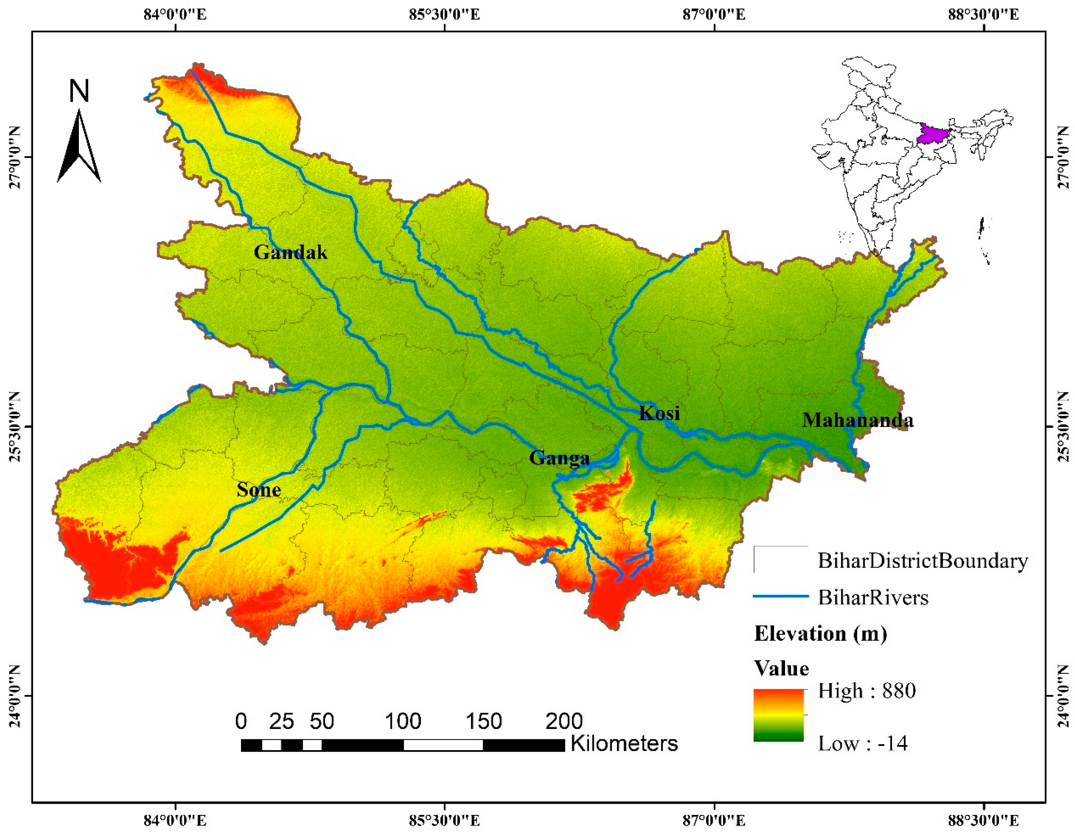
2.1. Study Area

Bihar, the 3rd most populous state in eastern India, with a population of over 120 million, has been taken up as the area of interest (Figure 1). The state is divided into 37 districts for administrative purposes. Bihar lies between 24°37′58″ N to 27°33′86″ N latitude and between 83°21′47″ E to 88°19′41″ E longitude. The Ganges River bifurcates the landlocked state, flowing from west to east. The states of Uttar Pradesh, West Bengal, and Jharkhand are in the west, east, and south, respectively, and the country of Nepal is in the north, which surrounds the state of Bihar. The state’s topography is relatively flat, with the climatic conditions remaining hot and humid for most of the year, as the state falls in the subtropical and temperate zone. The region has four seasons, namely the cold weather season (December to February), hot weather season (March to May), southwest monsoon (June to September), and retreating southwest monsoon (October to November). The state’s economy is primarily agriculture-driven, with rice being the primary crop. Bihar is the most flood-prone state in India [38], particularly in the northern parts, where the Kosi River is infamously dubbed as the ‘Sorrow of Bihar’. In contrast, the southern parts of Bihar are drought-prone [29]. The composite water index [19] depicts the state’s poorest performance in achieving the sustainable development goals (SDGs) [39].

2.2. Precipitation Data

Global climate change significantly impacts precipitation, making it a crucial parameter for analysis. The India Meteorological Department Gridded Precipitation (IMDGP) data (0.25° × 0.25°) at all the one hundred thirty-three grids in the study area, was obtained (https://www.imdpune.gov.in (accessed on 1 March 2022)) for the years 1901–2020 [40]. The data was prepared by interpolating the rainfall data from 6955 stations across India [40]; hence, there is no missing value. Preprocessing is performed in the Python programming environment to prepare a time series for each grid point. The trend tests were performed using the Pymannkendall library. The topo-to-raster interpolation technique is used to interpolate hydrologically correct raster surfaces from the results in ArcGIS 10.4.

2.3. Global Climate Models

Global climate models (GCMs) are an essential tool for analyzing scenario-based precipitation variability patterns, which is essential for planning water resource management, agricultural practice, and flood risk assessment. Thirteen global climate models from the latest Coupled Model Intercomparison Project Phase 6 (CMIP6) are used in the present study (https://cds.climate.copernicus.eu (accessed on 21 December 2023)). The present analysis utilizes the CMIP6s first ensemble member r1i1l1f1 and the historical, SSP370, and SSP585 scenarios. The GCMs are chosen such that all the historical and future scenario data are available for the study area. Information about the GCMs (model name and spatial resolution) chosen for this study is provided in Table 1. The data from GCMs is processed in a Python programming environment using the xarray library. This library is robust in dealing with the Network Common Data Format (netCDF), which is essentially multi-dimensional arrays commonly used as climate model output format. The GCMs are checked for consistency with the Gregorian calendar to ensure that leap days are considered during preprocessing.

2.4. Shared Socioeconomic Pathways

The Shared Socioeconomic Pathways (SSP) [41]) have replaced the Representative Concentration Pathways (RCP) scenarios within the CMIP6 framework. Unlike their predecessors, the RCP, the SSP scenarios integrate socioeconomic factors into climate projections and align with specific radiative forcing levels for 2100. The five SSPs provide distinct narratives that span a wide range of possible future developments, with SSP1 assuming a sustainable path and SSP5 assuming a world heavily reliant on fossil fuels and high greenhouse gas emissions. In the present study, SSP370 and SSP585 have been considered for analysis, which depict futures with less emphasis on environmental sustainability. The scenarios are chosen as they represent the trajectory of developing countries like India, which are in a phase of significant economic transformation and often rely on fossil fuels for growth. SSP370 is a scenario of high challenges to mitigation and medium challenges to adaptation, with a radiative forcing of 7.0 W/m2 by the end of the century. At the same time, SSP585 represents a future with very high greenhouse gas emissions, characterized by a heavy reliance on fossil fuels.

2.5. Methodology

The methods used in the study are presented in this section. Locally weighted scatterplot smoothing (LOWESS) was applied to the IMDGP dataset for the initial detection of trends in the long-term dataset. A smooth curve is fitted through the dataset using weighted regression in this method. Based on further change point detection tests, the time series is split into two epochs, and the Modified Mann–Kendall trend test is performed for trend analysis. Centroidal day analysis is performed to assess the temporal pattern of rainfall, while multivariate clustering is performed to analyze spatiotemporal variations in the region. All the GCMs are downscaled to the IMDGP spatial resolution (0.25° × 0.25°) using bilinear interpolation, which transforms all GCMs into finer data through interpolation from the four adjoining grid points and compared using probability density function (PDF) curves. The methods applied in this study are discussed further as follows.

2.5.1. Centroidal Day (CD)

Climate variations may cause a redistribution of rainfall throughout the year, resulting in temporal shifts. C D (Equation (1)) investigates such temporal shifts in annual (CDann) and monsoonal (CDmon) rainfall. C D may be considered the mean day for the annual or monsoonal rainfall over the entire year.
C D = i = 1 365 i × r i i = 1 365 r i
Here, ri is the daily rainfall on the ith day of the year or the monsoon season. CDs are calculated starting from 1 January every year. Equation (2) gives the shift in C D .
Shift   in   C D = length   of   time   series   ×   slope   of   C D   trend line

2.5.2. Modified Mann–Kendall Trend Test and Sen’s Slope Estimator

Non-parametric approaches, namely Modified Mann–Kendall (MMK) and Sen’s slope estimator, were carried out at a 5% significance level (α) to identify trends and slope in the datasets. The Mann–Kendall (MK) test does not depend on the distribution of the dataset while detecting monotonic trends. The test also has low sensitivity to abrupt changes in inhomogeneous datasets. A positive (negative) value of the normalized test statistic Z s indicates an increasing (decreasing) trend. The null hypothesis that no significant trend exists in the dataset is rejected if │ZS│ > 1.96. However, autocorrelated time series datasets need to be corrected for autocorrelation [42] between the rank of the observations ρ k . The magnitude of the identified trend is estimated using the non-parametric method of Sen’s slope estimator [43]. A detailed description of the equations is given in the Supplementary Materials.

2.5.3. Extreme Event Analysis

The maximum rainfall values at all the IMDGP points for each year are computed for extreme event analysis. The spatial average of these maximum values for a particular year gives the average maximum rainfall for the two epochs. Let R i j be the rainfall at the i t h grid during the j t h year. Then,
M j = m a x   R 1 j , R 2 j , , R N j
where M j is the maximum rainfall recorded in the j t h year across all the N grid points. Hence, the average maximum yearly rainfall M ¯ and the overall maximum rainfall M m a x for a total of Y years can be given by
M ¯ = 1 Y j = 1 Y M j
M m a x = m a x M 1 , M 2 , , M Y

2.5.4. Bayesian Model Averaging

A multi-model ensemble predicts future scenarios using Bayesian Model Averaging (BMA). Root Mean Square Error (RMSE) and Percentage Bias (P-bias) are utilized as the performance metrics for each GCM. The metrics are integrated into the BMA to calculate weights for each model, reflecting their relative performance. The metrics are first normalized for consistency (Equation (6)), then combined to create a combined performance metric (Equation (7)) by taking the average of the normalized values of RMSE and P-bias for each model.
N o r m a l i z e d   M e t r i c i = 1 M e t r i c i min M e t r i c + 1
C o m b i n e d   M e t r i c i = N o r m a l i z e d   R M S E i + N o r m a l i z e d   P b i a s i 2
The combined metric calculates the BMA weights (Equation (8)). The weight for each model is computed by dividing its combined metric by the sum of the combined metrics for all the models. The weights are finally applied to each model to create the weighted ensemble average for BMA (Equation (9)).
W e i g h t i = C o m b i n e d   M e t r i c i j = 1 n C o m b i n e d   M e t r i c j
E n s e m b l e   B M A = i = 1 n W e i g h t i × D a t a i

3. Results

3.1. Change Point Detection

Pettitt, SNHT, and Buishand range tests are carried out at a 5% significance level to detect abrupt change points in the long-term rainfall time series at all the IMDGP points. We took the year 1960 as the change point based on the results of these tests. LOWESS curves for different seasons and their variation pre- and post-1960 are shown in Figure 2. The results show marked shifts, especially during the pre-monsoon and post-monsoon seasons, suggesting that the rainfall had no monotonous trend; instead, there was some shift/change in the nature of the trend. Furthermore, the findings are in coherence with other studies related to change points [11,17,18] for the study area. Based on the identified change point, the time series is split into two epochs, first half (1901–1960) and the second half (1961–2020) for further analysis.

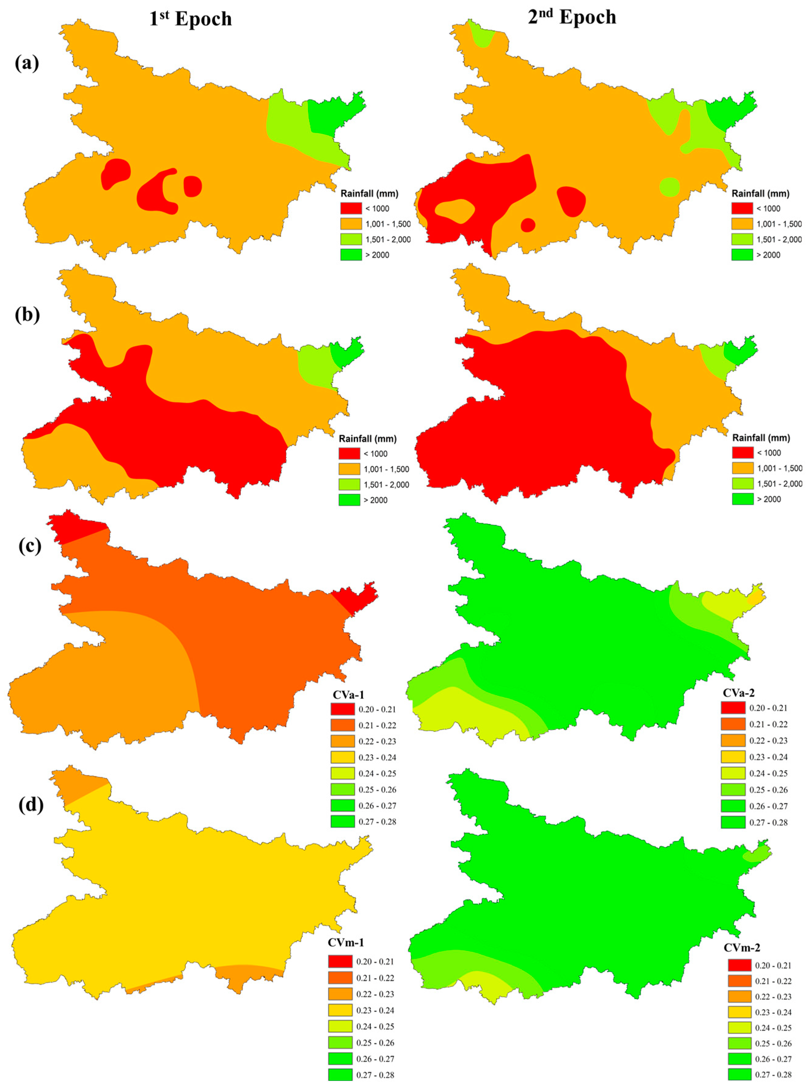
3.2. Overview of Rainfall in the Two Epochs

Figure 3a and Figure 3b, respectively, show the state’s annual and monsoonal spatial rainfall distribution. The northeastern parts of Bihar have the highest annual rainfall values (>2000 mm), while the rest of the area experiences an average annual rainfall of 1250 mm. Since monsoon months predominantly bring rainfall to the area, they also show a similar spatial trend in rainfall. Regions with low mean annual and monsoonal rainfall (<1000 mm) have expanded significantly in the second epoch, especially in the southwestern regions. The variability of annual and monsoonal rainfall is determined by the coefficient of variation (CV) (Figure 3a,b). There is a stark contrast in the variability between the first and second epochs, where the second epoch is predominated by higher values of CV that are absent in the first epoch. The annual and monsoonal variability seems to have increased by approximately 10% in all the districts in the second epoch. The districts of Patna, Vaishali, Samastipur, Darbhanga, Muzaffarpur, Sitamarhi, and Madhubani show more than 40% variability.

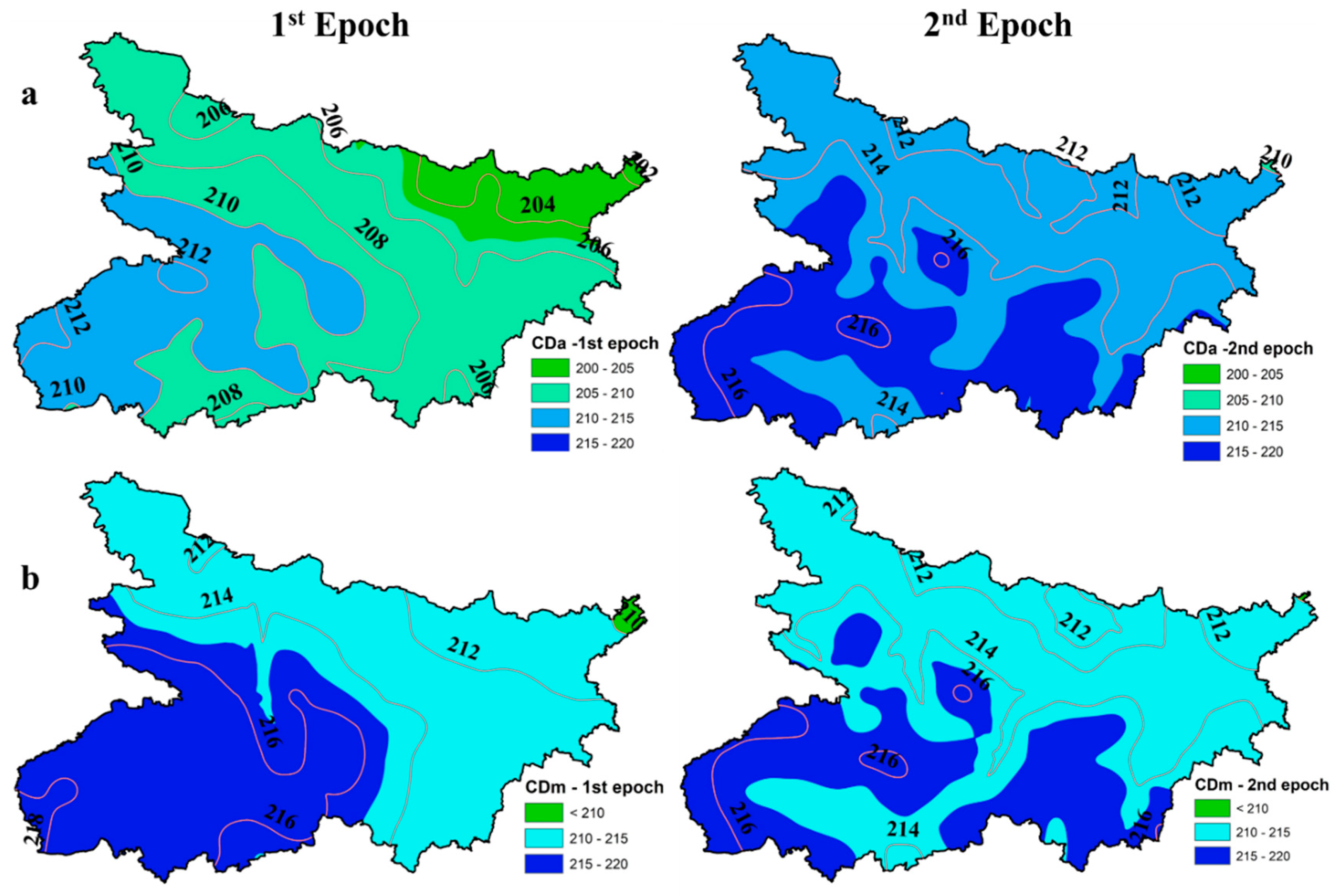
3.3. Shift in Annual and Monsoonal Rainfall

Figure 4 displays the annual (CDann) and the monsoonal (CDmon) shifts in rainfall. The results show definite shifts in the CDann values in the second half. The total rainfall can be assumed to have entered the state from the northeastern corner at around 201–203 days, and then progressed westwards in the first half. However, in the second half, the CDann values start at around 209–211 days, shifting on average by around 8–10 days. The nature of annual rainfall has completely changed between the two epochs. The contours appear to have increased values in the southward direction in the second half, as opposed to the earlier westward direction. Given the similar nature of annual and monsoonal rainfall, a correlation test between CDann and CDmon is carried out. The results show a stronger correlation between the two in recent years, particularly in the southern parts of the state, compared to the northern parts.

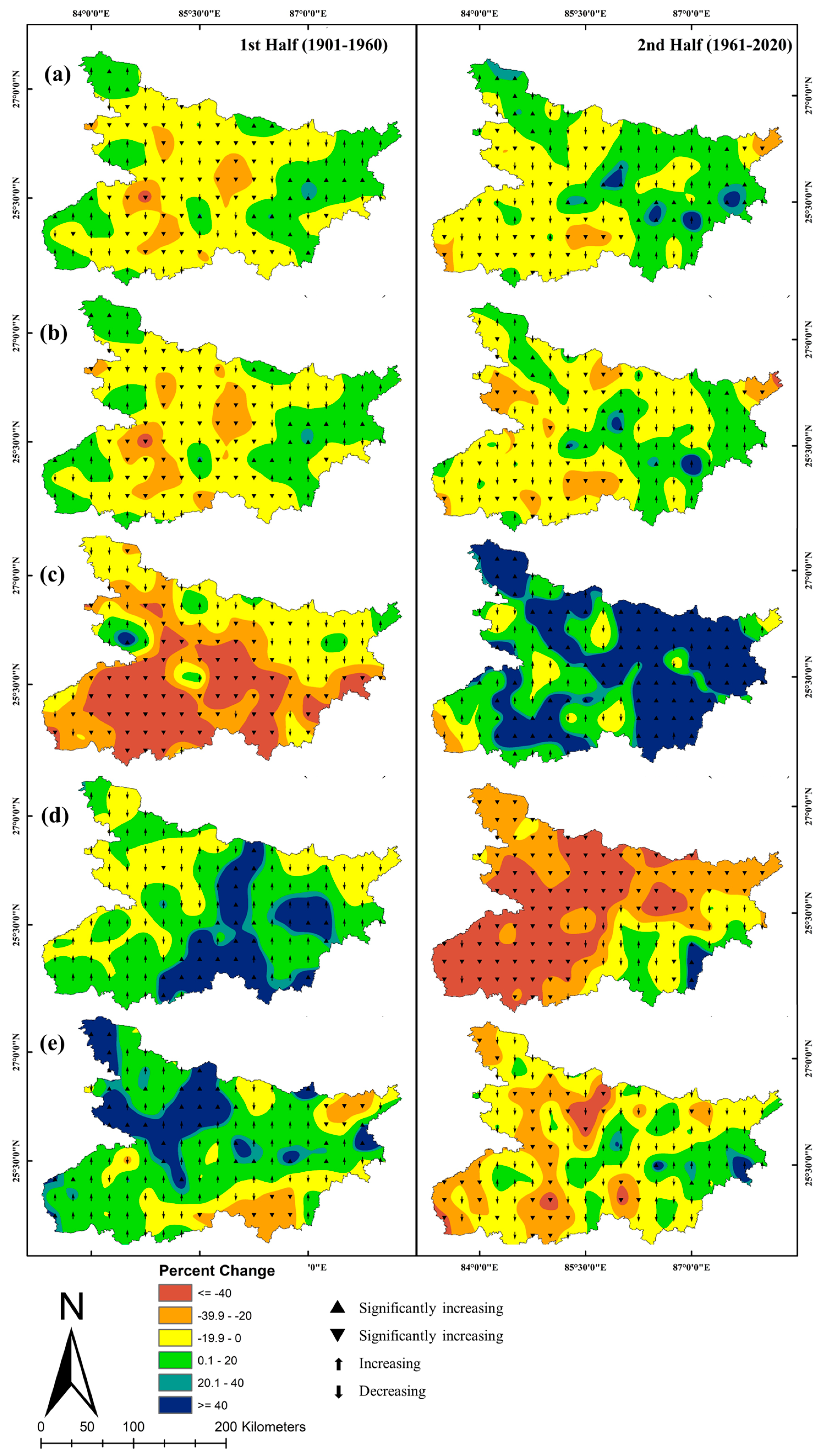
3.4. Trends in Annual and Seasonal Rainfall

The MMK test assesses the spatio-temporal trends for the annual and seasonal rainfall, and Figure 5 displays the percentage variability. Comparing the temporal variation in rainfall pre– and post–1960, a 4.4% increase in variability is seen for annual rainfall for the entire state. In total, 25 of the 37 districts in the state showed an increase in mean annual rainfall variability as compared to 19 for the mean monsoon rainfall. A significant decreasing trend is seen at 30 IMDGP points in the second epoch, compared to 51 in the first. A similar trend is observed for the monsoon rainfall, where 59 IMDGP points have a significant decreasing trend in the first epoch, compared to 31 in the second epoch. The eastern part of the state shows positive variability compared to the western regions.
Interestingly, the absolute variability of monsoon rainfall of approximately 5% is less than the annual average rainfall. In the second epoch, the pre-monsoon rainfall showed a 58.6% increase in temporal variability, with all districts showing significant changes. Notably, Khagaria and Munger have more than 100% variability. We observe a trend where the variability shifts from negative in the first epoch to positive in the second. However, all districts observe a change of –46.35% in the mean post-monsoon rainfall, indicating the opposite trend in variability. The mean winter rainfall shows mixed variability across all the districts. The northeastern corner of the state, occupied by the Kishanganj district, exhibits the least variability in rainfalls.

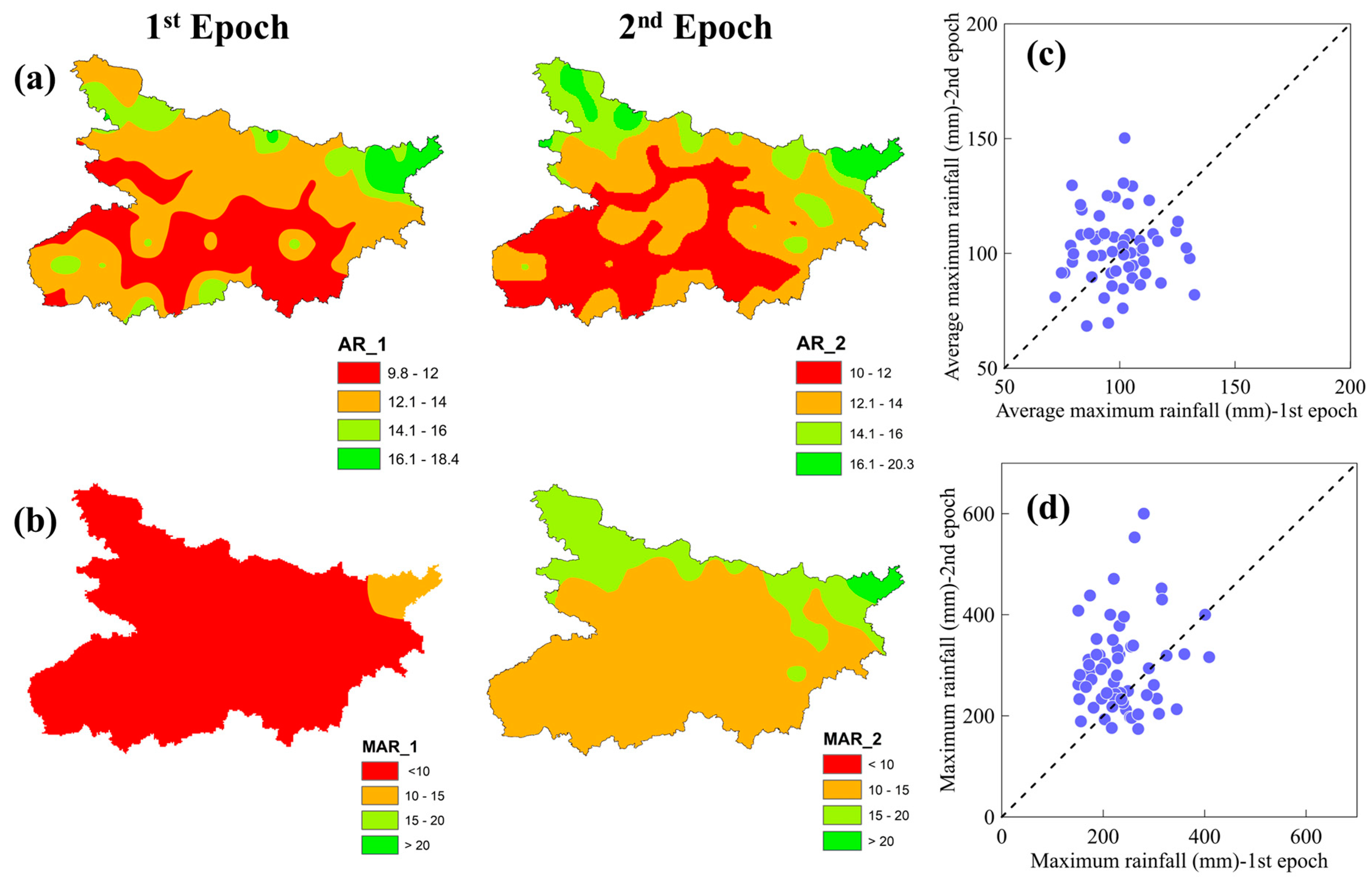
3.5. Trends in Extreme Rainfall Events and Rainfall Intensity

The MMK test is carried out to assess trends in the maximum one-day (1D), three-day (3D) and five-day (5D) rainfall. The results show a significantly increasing trend at twenty-three IMDGP points along the northeastern parts of the state, while the southwestern part recorded a significantly decreasing trend at twenty-three IMDGP points. A similar trend is observed for the 3D maximum rainfall. However, for the 5D maximum rainfall, a significant decreasing trend is observed at fifty-one IMDGP points, almost 40% of the total IMDGP points in the study area. The district of Bhagalpur, classified as prone to very high flood risk, shows the maximum increase in 1D (24.73%), 3D (23.57%), and 5D (21.69%) rainfall variability.
The annual and monsoonal daily mean rainfall intensity is computed because the extreme rainfall analysis does not reveal changes in rainfall intensity. The total rainfall, when divided by the number of wet days (rainfall ≠ 0), gives the daily rainfall intensity. We observe a significant increase (almost 20 days) in the number of annual dry days (rainfall = 0) for Gaya, Aurangabad, Darbhanga, Muzaffarpur, and Begusarai, while the monsoonal dry days have increased by approximately ten days for almost all the districts in the state in the second epoch. The southwestern parts show the most prominent increase in dry days, exhibiting a clear westward pattern. Comparing the annual rainfall intensity (AR) (Figure 6a), an increase in higher intensity (rainfall > 20 mm/day) areas is seen in north Bihar in the second epoch, while south Bihar is characterized by low intensity (rainfall < 10 mm/day) areas. However, changes in monsoonal rainfall intensity (MAR) (Figure 6b) are quite significant, with the entire rainfall characteristics observed to have changed. Almost the entire state shows a 50–75% increase in monsoonal rainfall intensity, which is consistent with the increase in the number of dry days. In particular, the northern districts of Bihar Paschim Champaran, Purba Champaran, Sitamarhi, Supaul, Araria, Kishanganj, and parts of Bhagalpur show an increase of more than 100%. Interestingly, although the average maximum precipitation (Figure 6c) for all the IMDGP points has increased by only 3 mm/day in the second epoch, the intensity and frequency of extreme rainfall events (Figure 6d) in the second epoch is considerably higher. Overall, a 60.6 mm/day (25.59%) increase in extreme rainfall is seen across the state.

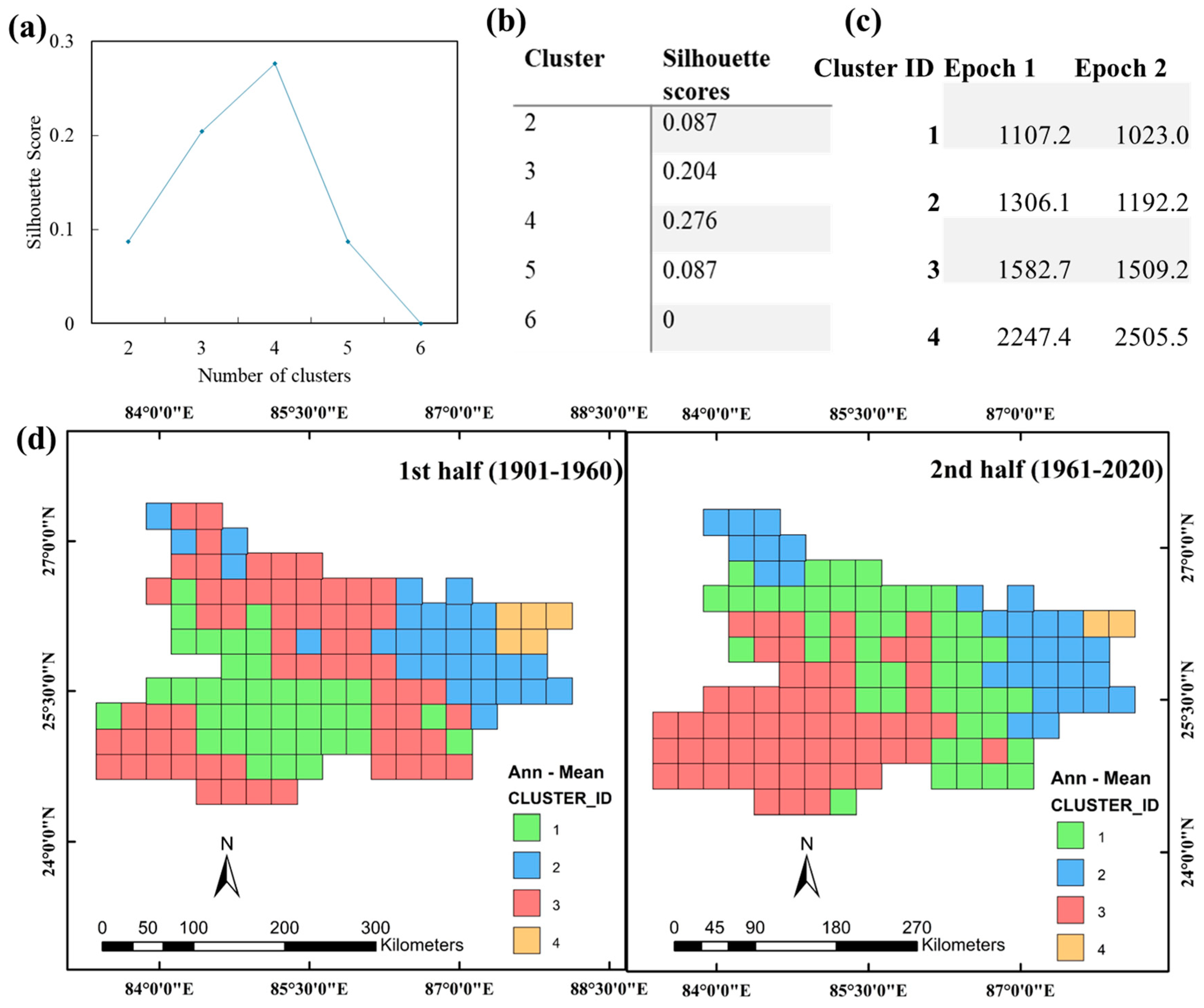
3.6. Changes in Regions with Homogeneous Rainfall

The precipitation pattern has changed across Bihar in the second epoch. Hence, a multivariate clustering approach brings out homogeneous precipitation regions using the mean annual rainfall for the two epochs. For clustering, the optimal number of clusters is determined by the silhouette score, a metric to estimate the goodness of the clustering technique. The optimal number of clusters corresponds to the silhouette score’s highest value. The analysis revealed the optimal number of clusters as four, corresponding to a silhouette score of 0.276 (Figure 7a,b). The results (Figure 7d) show that northeastern regions fall under similar clusters for the two epochs, with an approximate increase of 250 mm in mean annual rainfall (Figure 7c); however, moving westwards, the homogeneity patterns appear to have been altered in the second epoch. Cluster 3 appears to have shifted westwards in the second epoch, giving way to Cluster 1, thereby homogenizing the areas under Cluster 3. The low rainfall cluster 1 region shows a decrease in mean annual rainfall of almost 84 mm.

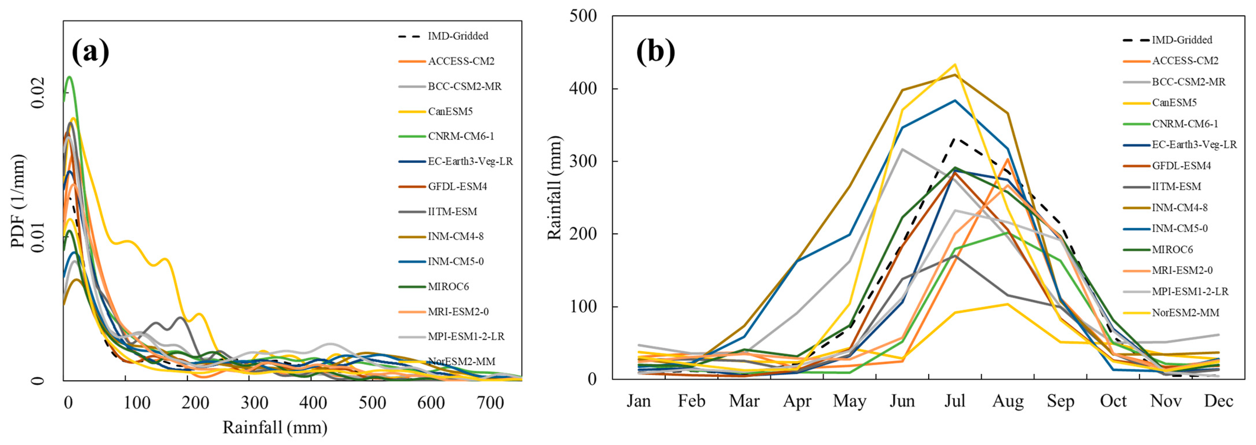
3.7. Comparison of GCMs with IMD Precipitation

Thirteen different GCMs are assessed in the present study to encompass a wide range of climate sensitivities, focusing on the relatively extreme SSP370 and the extreme SSP585 scenarios. Before forecasting future scenarios, it is imperative to understand the performance of GCMs compared to IMDGP. A baseline period of 1985–2014 is selected for assessing the performance of GCMs. The mean absolute error (MAE), probability density function (PDF), root mean square error (RMSE), and percentage bias (P-bias) analyze the comparison of the mean monthly precipitation of GCMs with the observed IMDGP dataset. PDF analysis suggests BCC-CSM2-MR, INM-CM4-8, INM-CM5-0, MIROC6, and NorESM2-MM tend to overestimate the precipitation, indicating that they predict higher rainfall more frequently. BCC-CSM2-MR, CanESM5, CNRM-CM6-1, EC-Earth-Veg-LR, GFDL-ESM4, IITM-ESM, MRI-ESM2-0, and MPI-ESM1-2-LR tend to underestimate rainfall, as evident by the left shift of the PDF curve compared to the IMD dataset. ACCESS-CM2 has a strong right skewness, which means it is better at predicting heavy rain events than BCC-CSM2-MR, CESM2, INM-CM4-8, and NorESM2-MM, which are also right-skewed.
MIROC6 and EC-Earth3-Veg-LR provide the best results, indicating that they closely follow the observed data in average conditions, but slightly overpredict the extreme rainfall values, as indicated by the peak and spread of the PDF curve.
The standard deviation for IMDGP is found to be 127.11. The values of standard deviation for GCMs (Table 2) ranges from 46.91 for CanESM5 to 160.07 for NorESM-MM indicating the uncertainty and model sensitivity. It is, hence, imperative to make future predictions after carefully selecting best performing models using statistical metric. Furthermore, we compute MAE, RMSE, and P-bias (Table 2) to evaluate the performance of GCMs in predicting average monthly rainfall values (Figure 8b). Standard deviation quantifies the uncertainty in model output. RMSE indicates the model’s accuracy, with lower values indicating better performance. P-bias measures the average tendency of the models to be larger or smaller than the observed data, with values closer to zero representing more accurate model bias.
EC-Earth3-Veg-LR, GFDL-ESM4, MIROC6, and MPI-ESM1-2-LR have the lowest MAE values of 46.11, 53.12, 52.20, and 47.78, respectively, suggesting closer agreement with the IMDGP data. CanESM5 has relatively high MAE (83.74) and RMSE (130.93), suggesting less accuracy in rainfall predictions. INM-CM4-8 and INM-CM5-0 have a significant positive P-bias, 60.78 and 38.07, respectively, indicating an overestimation of rainfall. CanESM5 (−55.05) and IIT-ESM (−41.86), on the other hand, underestimate rainfall, as evident by their low P-bias values.
ACCESS-CM2, BCC-CSM2-MR, CanESM5, IITM-ESM, INM-CM4-8, and INM-CM5-0 exhibit comparatively higher RMSE and P-Bias values compared to other GCMs. EC-Earth3-Veg-LR has the lowest RMSE (73.74), suggesting that its predictions are closest to the observed values and a relatively low P-bias (−14.97). NorESM2-MM has the second lowest P-bias (12.64), but has a higher RMSE value (113.34). MIROC6 shows a good balance between the RMSE (79.74) and P-bias (4.51), indicating minimal bias in the predictions. MPI-ESM1-2-LR has a slightly high negative P-bias (−23.58), but a low RMSE (78.52). The low bias of the EC-Earth3-Veg-LR, MIROC6, and MPI-ESM1-2-LR compared to others indicates their robustness in accurately simulating rainfall patterns across the different months. To make reliable climate predictions, a multi-model ensemble of the three models, EC-Earth-Veg-LR, MIROC6, and MPI-ESM1-2-LR, is performed using Bayesian model averaging (BMA), as explained in Section 2.5.4.

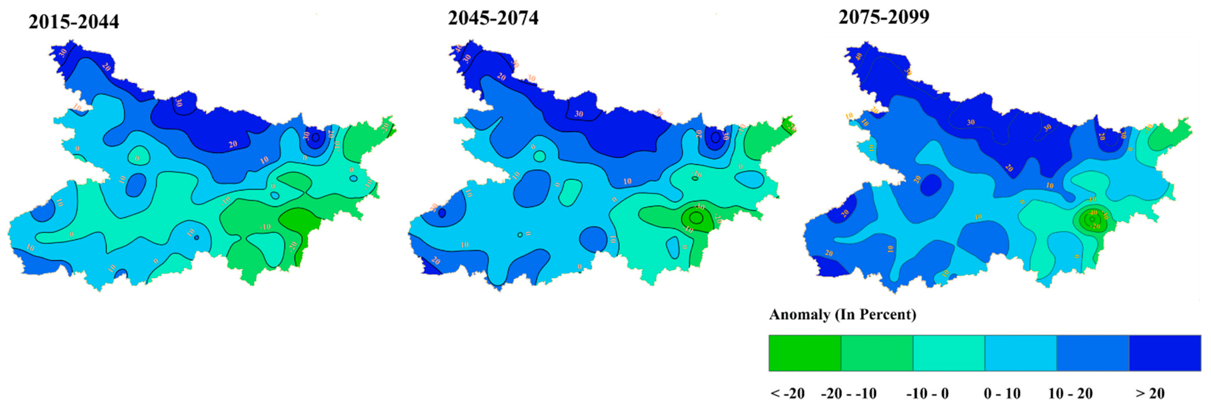
3.8. Bayesian Multi-Model Ensemble for Future Prediction

Figure 9 and Figure 10 show the mean annual precipitation in form of anomaly for the duration of 2015–2045, 2046–2075, and 2076–2099 for the multi model ensemble for the three models, EC-Earth3-Veg-LR, MIROC6, and MPI-ESM1-2-LR, using BMA under the SSP370 and SSP585 scenarios, respectively. We observe a general increase in rainfall across the state compared to the current trends, as shown by Figure 9. Interestingly, a low average annual rainfall (<750 mm) region in southwestern Bihar is seen for the duration of 2015–2045 for SSP370, as evident by the negative anomaly (Figure 9). For the subsequent duration, the region will, however, have a positive anomaly, except for the region over the Bhagalpur district (central-east), which is expected to have a negative anomaly. Regions in northern Bihar will continue to have a higher rainfall anomaly (>20%) under SSP370 and SSP585 scenarios, as evident by positive anomalies. The region of these positive anomalies will expand with the progress of time, with significant increase seen for SSP585 (Figure 10). The increase in region of very high anomaly (>30%) in both north and south Bihar is prominent for SSP585. However, even for SSP585, the central eastern and central western parts of Bihar show a negative rainfall anomaly (<−10%).

4. Discussion

Statistical analysis of rainfall in Bihar reveals substantial changes in spatiotemporal rainfall characteristics. Change point detection tests divide the time series into two epochs. The identification of 1960 as the change point year underlines the importance of historical climate data in understanding the regional impacts of global climate change. The analysis reveals a stark contrast between the precipitation patterns and seasonality of the first and second epochs. The second epoch is characterized by higher spatiotemporal variability, shifts in rainfall patterns, and an increase in the intensity and frequency of extreme events. For instance, the southwestern regions receive relatively low rainfall (<1000 mm), and this region of relatively low rainfall has expanded significantly (by almost 14 times) in the last 30 years compared to earlier years. The changes in rainfall patterns can explain why it is now one of the most drought-prone regions in the state [29]. Similarly, the increase in intense precipitation events by 25.6% has led to severe flooding in the state almost every year, calling for measures to enhance infrastructure resilience and disaster preparedness. In contrast, the high correlation values between CDann and CDmon indicate the dominance of monsoons as the source of rainfall and the diminishing contribution of rainfall from other seasons in southern Bihar. Consequently, strong reliance on monsoons for rainfall and the decreasing trends of annual rainfall have increased the drought risk in these regions. This is supported by the findings of rainfall intensity, where an increase in higher intensity rainfall (rainfall > 20 mm/day) areas is seen in north Bihar, while south Bihar sees an increase in low intensity (rainfall < 10 mm/day) rainfall areas.
Intense rainfall events and declining rainfall in southwestern Bihar could reduce water availability and drought-like conditions. This is a serious cause for concern as the drought-prone south primarily relies on rainfall for agriculture. Agriculture is a significant part of Bihar’s economy, contributing 26.51% to the state GDP [44] and supporting almost 90% of the population, directly or indirectly. These variabilities have put Bihar in a unique place, i.e., it can experience floods and drought at the same time, and despite being home to massive river systems, the state ranks worst in water resource management. The stark contrast in rainfall variability between the two epochs underscores the accelerating impact of climate change over time, and emphasizes the regional manifestation of the global climate phenomenon.
To further understand the implications of precipitation variability on hydrological components, alterations in water storage, surface runoff depth, and evapotranspiration are analyzed. The National Resources Soil Conservation-Curve Number (NRSC-CN) model is used to estimate total runoff across the state from 2001 to 2020. The equivalent water thickness from Gravity Recovery and Climate Experiment’s (GRACE) monthly mass grids is used to obtain water storage data for 2002–2017. Further, the MOD16A2.006 Terra Net Evapotranspiration (ET) 8-Day Global data at 500 m spatial resolution are used for ET estimation.
An approximately 60 mm (13.43%) increase in average runoff in Bihar is seen from 2001 to 2020 (Figure 11), during which the annual rainfall mainly decreases. Such a trend can be explained by the rapid urbanization and increase in agricultural lands; land use features that result in higher runoff as compared to vegetation and forest. Coupling the increase in surface runoff with the increase in rainfall intensity, especially along the northern parts of Bihar, would lead to more significant flood risks. In 2019, severe flooding inundated more than 35% of the districts of Patna and Bhagalpur. A decrease of 242.3 mm in water storage is seen during the 2002–2017 period, which correlates strongly (0.56) with annual rainfall during that period. NITI Aayog’s composite water index study ranked the state last due to its failure to achieve sustainable development goals (SDGs), poor management of river basins, and lack of regulation over water exploitation.
Further observations reveal a 118.86 mm decrease in ET, an essential component of the hydrological cycle. Water availability (mainly precipitation) controls ET over the region, with annual precipitation and ET weakly correlated by a value of 0.28. The analysis reveals the sensitive state of rainfall in Bihar and the need to pave the way for more robust water resource management in the region.
Consequently, analyzing GCMs, especially the extreme scenarios of SSP370 and SSP585, is critical to planning adequate water management policies for the future. The extreme scenarios are chosen, as they represent the upper bounds of plausible future pathways of a developing region like Bihar. The minimal difference in minimum values across the thirteen GCMs analyzed using PDF suggests that most models can capture low precipitation events similarly to the IMD-gridded dataset. However, EC-Earth3-Veg-LR, INM-CM4-8, INM-CM5-0, MIROC-ES2L, and MPI-ESM1-2-LR cannot capture the extremes well. EC-Earth3-Veg-LR, MIROC6, and MPI-ESM1-2-LR are the best-performing models for the region, as indicated by the low MAE, RMSE, and P-Bias values. A Bayesian multi-model ensemble for these three GCMs is prepared to capture a broader range of possible outcomes and reduce uncertainty. The rainfall anomaly derived from the multi-model ensemble predicts increased precipitation in the flood-prone northern region for both SSP370 and SSP585 scenarios, indicating a likely increase in flood risk in the sensitive region. The region under a very high rainfall anomaly (>30%) will increase in area for SSP585 in both south and north Bihar. For SSP370, the increase in regions of low annual rainfall in the drought-prone south and southwest of Bihar for 2015–2045 might increase the agricultural drought risk.
Overall, the significant findings of the study can be elucidated as:
  • An evident change in precipitation trend was observed around the year 1960. There is a clear shift in the trend of southwest monsoons over the region, as evidenced by the rainfall variability during the different seasons pre- and post-1960. The nature of the pre-monsoon and post-monsoon seasons has flipped over the area in recent years.
  • The nature of annual rainfall has completely changed between the two epochs, as evident by CDann.
  • An increase in dry days has increased in monsoonal rainfall intensity. The frequency and intensity of extreme rainfall increased in the second epoch. Overall, the state experienced an increase in extreme rainfall of 60.6 mm/day (25.59%). Further, an increase in higher intensity (rainfall > 20 mm/day) areas is seen in north Bihar, while south Bihar sees an increase in low intensity (rainfall < 10 mm/day) areas.
  • There is a marked variability in the state as one goes from east to west in terms of homogeneity (defined by clusters) and hydrological extremes as one goes from north to south. This leaves Bihar in a unique position, with an imminent need to combat the climate variability-induced risk to water resources for sustainable development.
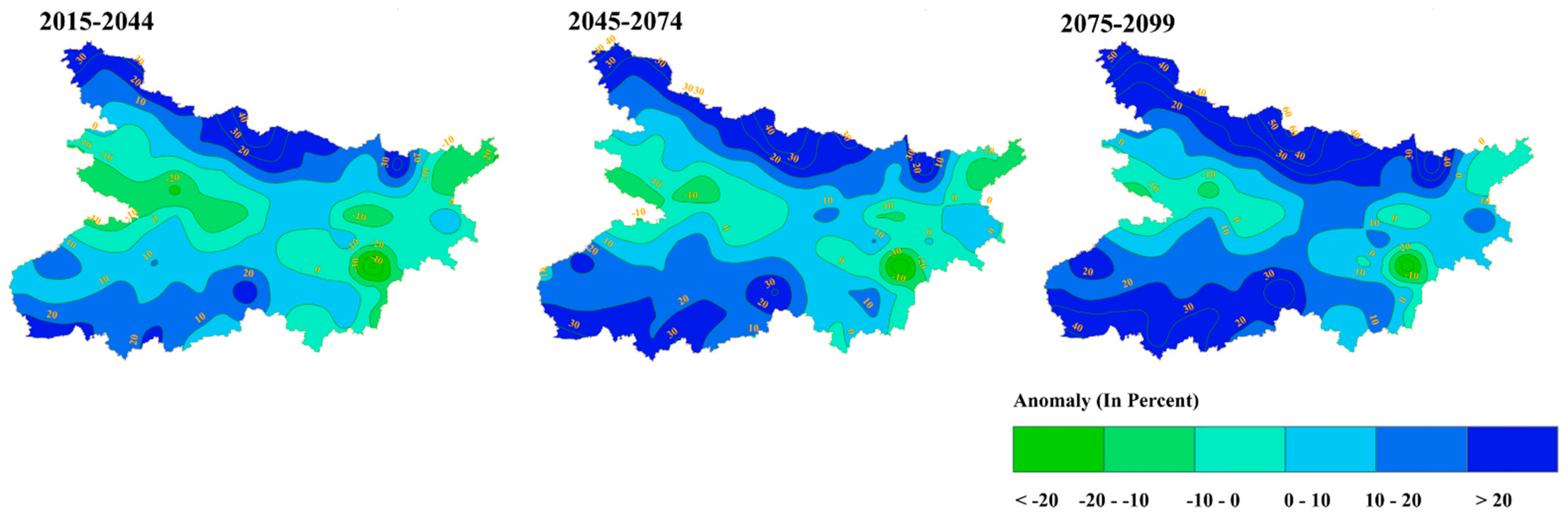
  • EC-Earth3-Veg-LR, MIROC6 and MPI-ESM1-2-LR are the best-performing models for the region. A Bayesian multi-model ensemble suggests that south Bihar will receive low rainfall for the duration of 2015–2045, hence increasing the drought risk.

5. Conclusions

The present study gives a comprehensive spatiotemporal evaluation of the variability of rainfall; trends in annual, seasonal, and extreme rainfall; changes in rainfall patterns and the reliability of GCMs in predicting the rainfall variability over the state of Bihar in India; and its implications on surface runoff and agriculture. We observe significant spatiotemporal variations in rainfall, with the change point year indicating a divergence in rainfall trends and characteristics, including a shift in seasonality across all seasons, particularly during the monsoon. The observed changes might be attributed to the combined impact of increased urbanization and the associated climate change, though further investigation is necessary to delineate their respective contribution. The study highlights an increase in extreme dry and wet events, suggesting prolonged droughts and more frequent flooding. Projections based on the SSP370 scenario of the BMS multi-model ensemble indicate a decrease in rainfall until 2045, followed by an increase until 2100. The predictions underscore the importance of informed water resource management policies for a sustainable future. The findings further suggest that larger climate phenomena exert a cyclic effect on rainfall over the state, as evidenced by examining climate scenarios, which need further assessment for a deeper understanding of the regional climatic variability. Additionally, exploring the role of El-Nino Southern Oscillation and Indian Ocean Dipole could provide valuable insights into the observed cyclic nature of regional rainfall.

Supplementary Materials

The following supporting information can be downloaded at: https://0-www-mdpi-com.brum.beds.ac.uk/article/10.3390/hydrology11040050/s1, File S1: Supplementary—Mann-Kendall test.

Author Contributions

A.R., V.K. and O.P.: Conceptualization, methodology, formulation, Investigation, Original draft preparation, and Validation; O.P.: Supervision; A.R. and O.P.: Reviewing, Editing, and Revision; A.R. and O.P.: Visualization and Editing. All authors have read and agreed to the published version of the manuscript.

Funding

This research received no external funding.

Data Availability Statement

All the data used in the study are open-source and appropriate links to the data sources are given in the manuscript.

Conflicts of Interest

The authors declare no conflicts of interest.

References

  1. Islam, T.; Rico-Ramirez, M.A.; Han, D.; Srivastava, P.K.; Ishak, A.M. Performance evaluation of the TRMM precipitation estimation using ground-based radars from the GPM validation network. J. Atmos. Sol.-Terr. Phys. 2012, 77, 194–208. [Google Scholar] [CrossRef]
  2. Gajbhiye, S.; Meshram, C.; Singh, S.K.; Srivastava, P.K.; Islam, T. Precipitation trend analysis of Sindh River basin, India, from 102-year record (1901–2002). Atmos. Sci. Lett. 2016, 17, 71–77. [Google Scholar] [CrossRef]
  3. Srivastava, P.K.; Han, D.; Rico-Ramirez, M.A.; Islam, T. Sensitivity and uncertainty analysis of mesoscale model downscaled hydro-meteorological variables for discharge prediction. Hydrol. Process. 2014, 28, 4419–4432. [Google Scholar] [CrossRef]
  4. Res, C.; Trenberth, K.E. Changes in precipitation with climate change. Clim. Res. 2011, 47, 123–138. [Google Scholar] [CrossRef]
  5. Ashok, K.; Guan, Z.; Saji, N.H.; Yamagata, T. Individual and combined influences of ENSO and the Indian Ocean Dipole on the Indian summer monsoon. J. Clim. 2004, 17, 3141–3155. [Google Scholar] [CrossRef]
  6. Torrence, C.; Webster, P.J. Interdecadal changes in the ENSO-monsoon system. J. Clim. 1999, 12 Pt 2, 2679–2690. [Google Scholar] [CrossRef]
  7. Dash, S.K.; Jenamani, R.K.; Kalsi, S.R.; Panda, S.K. Some evidence of climate change in twentieth-century India. Clim. Chang. 2007, 85, 299–321. [Google Scholar] [CrossRef]
  8. Mondal, A.; Khare, D.; Kundu, S. Spatial and temporal analysis of rainfall and temperature trend of India. Theor. Appl. Climatol. 2015, 122, 143–158. [Google Scholar] [CrossRef]
  9. Dash, S.K.; Kulkarni, M.A.; Mohanty, U.C.; Prasad, K. Changes in the characteristics of rain events in India. J. Geophys. Res. Atmos. 2009, 114, 1–12. [Google Scholar] [CrossRef]
  10. Guhathakurta, P.; Rajeevan, M.; Sikka, D.R.; Tyagi, A. Observed changes in southwest monsoon rainfall over India during 1901–2011. Int. J. Climatol. 2015, 35, 1881–1898. [Google Scholar] [CrossRef]
  11. Gnanaseelan, C.; Mujumdar, M.; Kulkarni, A.; Chakraborty, S.; Sciences, E. Assessment of Climate Change over the Indian Region; Springer: Berlin/Heidelberg, Germany, 2020. [Google Scholar] [CrossRef]
  12. Naidu, C.V.; Srinivasa Rao, B.R.; Bhaskar Rao, D.V. Climatic trends and periodicities of annual rainfall over India. Meteorol. Appl. 1999, 6, 395–404. [Google Scholar] [CrossRef]
  13. Zhang, L.; Zhou, T. An assessment of monsoon precipitation changes during 1901–2001. Clim. Dyn. 2011, 37, 279–296. [Google Scholar] [CrossRef]
  14. IPCC. Summary for Policymakers: A Report of Working Group I of the Intergovernmental Panel on Climate Change; IPCC: Geneva, Switzerland, 2007. [Google Scholar]
  15. Guhathakurta Pulak Khedikar, S.; Menon, P.; Prasad, A.K.; Sable, S.T.; Advani, S.C. Climate Research and Services Observed Rainfall Variability and Changes over Assam State. IMD Annu. Rep. 2020, 16, 28. [Google Scholar]
  16. Praveen, B.; Talukdar, S.; Shahfahad Mahato, S.; Mondal, J.; Sharma, P.; Islam AR, M.T.; Rahman, A. Analyzing trend and forecasting of rainfall changes in India using non-parametrical and machine learning approaches. Sci. Rep. 2020, 10, 10342. [Google Scholar] [CrossRef]
  17. Warwade, P.; Tiwari, S.; Ranjan, S.; Chandniha, S.K.; Adamowski, J. Spatio-temporal variation of rainfall over Bihar State, India. J. Water Land Dev. 2018, 36, 183–187. [Google Scholar] [CrossRef]
  18. Zakwan, M.; Ara, Z. Statistical analysis of rainfall in Bihar. Sustain. Water Resour. Manag. 2019, 5, 1781–1789. [Google Scholar] [CrossRef]
  19. NITI Aayog. Composite Water Mangement Index. 2019; pp. 11–13. Available online: http://niti.gov.in/writereaddata/files/new_initiatives/presentation-on-CWMI.pdf (accessed on 23 June 2023).
  20. Tesfaye, K.; Aggarwal, P.K.; Mequanint, F.; Shirsath, P.B.; Stirling, C.M.; Khatri-Chhetri, A.; Rahut, D.B. Climate variability and change in Bihar, India: Challenges and opportunities for sustainable crop production. Sustainability 2017, 9, 1998. [Google Scholar] [CrossRef]
  21. Rashiq, A.; Prakash, O. Assessment of Spatio-temporal variability of climate in the lower Gangetic alluvial plain. Environ. Monit. Assess. 2023, 195, 945. [Google Scholar] [CrossRef] [PubMed]
  22. Bommaraboyina, P.R.; Daniel, J.; Abbhishek, K. Book Review: Climate Change and Agriculture in India: Impact and Adaptations. Front. Clim. 2020, 2, 576004. [Google Scholar] [CrossRef]
  23. NRSC. Flood Hazard Atlas–Bihar; NRSC: Hyderabad, India, 2020; p. 137.
  24. Saharia, M.; Jain, A.; Baishya, R.R.; Haobam, S.; Sreejith, O.P.; Pai, D.S.; Rafieeinasab, A. India flood inventory: Creation of a multi-source national geospatial database to facilitate comprehensive flood research. Nat. Hazards 2021, 108, 619–633. [Google Scholar] [CrossRef]
  25. Bhatt, C.M.; Srinivasa Rao, G.; Manjushree, P.; Bhanumurthy, V. Space based disaster management of 2008 Kosi floods, North Bihar, India. J. Indian Soc. Remote Sens. 2010, 38, 99–108. [Google Scholar] [CrossRef]
  26. Kumar, S.; Roshni, T.; Kumar, A.; Jayakumar, D. GIS-Based Drought Assessment in Climate Change Context: A Case Study for Sone Command, Bihar. J. Inst. Eng. Ser. A 2021, 102, 199–213. [Google Scholar] [CrossRef]
  27. Sinha, R.; Bapalu, G.V.; Singh, L.K.; Rath, B. Flood risk analysis in the Kosi river basin, north Bihar using multi-parametric approach of Analytical Hierarchy Process (AHP). J. Indian Soc. Remote Sens. 2008, 36, 335–349. [Google Scholar] [CrossRef]
  28. Tripathi, G.; Parida, B.R.; Pandey, A.C. Spatio-temporal rainfall variability and flood prognosis analysis using satellite data over North Bihar during the August 2017 flood event. Hydrology 2019, 6, 38. [Google Scholar] [CrossRef]
  29. Brakenridge, G.R. Global Active Archive of Large Flood Events. In Dartmouth Flood Observatory; University of Colorado: Boulder, CO, USA, 2016; Available online: http://floodobservatory.colorado.edu/Archives/ (accessed on 23 June 2023).
  30. Yaduvanshi, A.; Srivastava, P.K.; Pandey, A.C. Integrating TRMM and MODIS satellite with socioeconomic vulnerability for monitoring drought risk over a tropical region of India. Phys. Chem. Earth 2015, 83–84, 14–27. [Google Scholar] [CrossRef]
  31. Krishna Kumar, K.; Rupa Kumar, K.; Ashrit, R.G.; Deshpande, N.R.; Hansen, J.W. Climate impacts on Indian agriculture. Int. J. Climatol. 2004, 24, 1375–1393. [Google Scholar] [CrossRef]
  32. Khanal, A.R.; Mishra, A.K. Enhancing food security: Food crop portfolio choice in response to climatic risk in India. Glob. Food Secur. 2017, 12, 22–30. [Google Scholar] [CrossRef]
  33. Sharma, A.; Maharana, P.; Sahoo, S.; Sharma, P. Environmental change and groundwater variability in South Bihar, India. Groundw. Sustain. Dev. 2022, 19, 100846. [Google Scholar] [CrossRef]
  34. Sen, S. Climate variability and migration in Bihar: An empirical analysis. Int. J. Disaster Risk Reduct. 2024, 103, 104301. [Google Scholar] [CrossRef]
  35. Das, L.; Bhowmick, S.; Meher, J.K.; Mahdi, S.S. CMIP5 based past and future climate change scenarios over South Bihar, India. J. Earth Syst. Sci. 2023, 132, 8. [Google Scholar] [CrossRef]
  36. Jha, R.K.; Kalita, P.K.; Cooke, R.A. Assessment of climatic parameters for future climate change in a major agricultural state in India. Climate 2021, 9, 111. [Google Scholar] [CrossRef]
  37. Kumar, S.; Roshni, T.; Kahya, E.; Ghorbani, M.A. Climate change projections of rainfall and its impact on the cropland suitability for rice and wheat crops in the Sone river command, Bihar. Theor. Appl. Climatol. 2020, 142, 433–451. [Google Scholar] [CrossRef]
  38. IWMI. Chapter 1: Present Scenario and Need for Index Based Flood Insurance in Bihar. In Index Based Flood Insurance (IBFI); IWMI: New Delhi, India, 2018. [Google Scholar]
  39. GoI. SDG India Index & Dashboard 2020–21 Report. In Partnerships in the Decade of Action; Niti Aayog: New Delhi, India, 2021; p. 348. Available online: https://niti.gov.in/writereaddata/files/SDG_3.0_Final_04.03.2021_Web_Spreads.pdf (accessed on 1 June 2023).
  40. Pai, D.S.; Sridhar, L.; Rajeevan, M.; Sreejith, O.P.; Satbhai, N.S.; Mukhopadhyay, B. Development of a new high spatial resolution (0.25° × 0.25°) long period (1901–2010) daily gridded rainfall data set over India and its comparison with existing data sets over the region. Mausam 2014, 65, 1–18. [Google Scholar] [CrossRef]
  41. Riahi, K.; van Vuuren, D.P.; Kriegler, E.; Edmonds, J.; O’Neill, B.C.; Fujimori, S.; Bauer, N.; Calvin, K.; Dellink, R.; Fricko, O.; et al. The Shared Socioeconomic Pathways and their energy, land use, and greenhouse gas emissions implications: An overview. Glob. Environ. Chang. 2017, 42, 153–168. [Google Scholar] [CrossRef]
  42. Hamed, K.; Rao, R. A modified Mann-Kendall trend test for autocorrelated data. J. Hydrol. Eng. 1998, 213, 346–360. [Google Scholar] [CrossRef]
  43. Sen, P.K. Estimates of the Regression Coefficient Based on Kendall’s Tau. J. Am. Stat. Assoc. 1968, 2013, 37–41. [Google Scholar] [CrossRef]
  44. Salam, A.; Anwer, E.; Alam, S. Agriculture and the Economy of Bihar. Int. J. Sci. Res. Publ. 2013, 3, 1–19. [Google Scholar]
Figure 1. Geographical location of the study area along with color defined elevation levels and major rivers.
Hydrology 11 00050 g001
Figure 2. LOWESS curve on (a) annual rainfall, (b) monsoon rainfall, (c) pre-monsoon rainfall, (d) post-monsoon rainfall, and (e) winter rainfall, with the horizontal dotted line representing the year of change point.
Hydrology 11 00050 g002
Figure 3. Spatial distribution of mean (a) annual and (b) monsoonal rainfall, and spatial variability (in terms of coefficient of variation) for the (c) annual and (d) monsoonal rainfall for the 1st and 2nd epochs.
Hydrology 11 00050 g003
Figure 4. Contour map showing the variation in the centroidal day along with their values represented by contours for (a) annual and (b) monsoonal rainfall across the two epochs.
Hydrology 11 00050 g004
Figure 5. Spatial changes in the (a) annual rainfall, (b) monsoon rainfall, (c) pre–monsoon rainfall, (d) post–monsoon rainfall and (e) winter rainfall for the two epochs at 5% significance level.
Hydrology 11 00050 g005
Figure 6. Maps showing the spatial variation in (a) mean annual and (b) mean monsoonal rainfall intensities during the 1st and 2nd epochs. The scatterplot represents the (c) average maximum rainfall and (d) maximum rainfall across the state for the two epochs.
Hydrology 11 00050 g006
Figure 7. (a) Line chart showing the number of clusters, (b) the actual silhouette scores for different clusters, (c) rainfall values (mm) for the different clusters, and (d) results of multivariate rainfall clusters for the two epochs.
Hydrology 11 00050 g007
Figure 8. (a) PDFs comparing mean monthly observed IMD gridded precipitation to the GCMs. (b) Comparison of mean monthly IMD gridded and GCM precipitation.
Hydrology 11 00050 g008
Figure 9. Variation in rainfall anomaly (as percentage deviation from base period rainfall 1985−2014) for 2015−2045, 2046−2075, and 2076−2099 using the Bayesian averaged multi-model ensemble for the SSP370 scenario.
Hydrology 11 00050 g009
Figure 10. Variation in rainfall anomaly (as percentage deviation from base period rainfall 1985−2014) for 2015−2045, 2046−2075, and 2076−2099 using the Bayesian averaged multi-model ensemble for the SSP585 scenario.
Hydrology 11 00050 g010
Figure 11. Variation in water storage (GRACE data), evapotranspiration (AET) and runoff with rainfall for 2001−2020.
Hydrology 11 00050 g011
Table 1. Information about the GCMs used in the present study.
Sl. No.GCMInstitution, CountryResolution
1ACCESS-CM2Australian Community Climate and Earth System Simulator, Australia1.9° × 1.3°
2BCC-CSM2-MRBeijing Climate Center, China1.1° × 1.1°
3CanESM5Canadian Centre for Climate Modelling and Analysis, Canada2.8° × 2.8°
4CNRM-CM6-1National Centre for Meteorologic Research, France1.4° × 1.4°
5EC-Earth3-Veg-LREurope0.7° × 0.7°
6GFDL-ESM4Geophysical Fluid Dynamics Laboratory, USA1.3° × 1.0°
7IITM-ESMIndian Institute of Tropical Meteorology1.91° × 1.87°
8INM-CM4-8Marchuk Institute of Numerical Mathematics, Russia2.0° × 1.5°
9INM-CM5-02.0° × 1.5°
10MIROC6The University of Tokyo, National Institute for Environmental Studies, and Japan Agency for Marine-Earth Science and Technology, Japan1.4° × 1.4°
11MPI-ESM1-2-LRMax Plank Institute, Germany1.9° × 1.9°
12MRI-ESM2-0Meteorological Research Institute, Japan1.1° × 1.1°
13NorESM2-MMNorwegian Meteorological Institute, Norway0.94° × 1.25°
Table 2. Comparison of the 13 GCMs with the IMD gridded data using root mean square error (RMSE) and percentage-bias (P-bias).
Global Climate ModelsStd. Dev.MAERMSEP-Bias
1ACCESS-CM296.9466.99105.37−32.54
2BCC-CSM2-MR124.5081.36121.1117.47
3CanESM546.9183.74130.93−55.05
4CNRM-CM6-184.4662.1199.70−38.33
5EC-Earth3-Veg-LR109.2446.1173.74−14.97
6GFDL-ESM4104.2953.1287.5−26.29
7IITM-ESM67.3562.95102.63−41.86
8INM-CM4-8156.7393.37125.2960.78
9INM-CM5-0142.4474.71105.0138.07
10MIROC6117.9952.2079.744.51
11MPI-ESM1-2-LR91.5947.7878.52−23.58
12MRI-ESM2-0100.1957.7588.98−22.4
13NorESM2-MM160.0769.99113.3412.64
Disclaimer/Publisher’s Note: The statements, opinions and data contained in all publications are solely those of the individual author(s) and contributor(s) and not of MDPI and/or the editor(s). MDPI and/or the editor(s) disclaim responsibility for any injury to people or property resulting from any ideas, methods, instructions or products referred to in the content.

