Uncertainty in Catchment Delineations as a Result of Digital Elevation Model Choice


Institut für Geographie, Friedrich-Schiller-Universität Jena, Löbdergraben 32, 07743 Jena, Germany
*
Author to whom correspondence should be addressed.
Hydrology 2019, 6(1), 13; https://0-doi-org.brum.beds.ac.uk/10.3390/hydrology6010013
Submission received: 22 December 2018
/
Revised: 27 January 2019
/
Accepted: 31 January 2019
/
Published: 1 February 2019
Abstract
:Nine digital elevation model (DEM) datasets were used for separate delineations of the Nam Co, Tibet catchment and its subcatchments, and these delineated areas were compared using the highest resolution dataset, TanDEM-X 12 m, as a baseline. The mean delineated catchment area was within 0.1% percent of the baseline delineation, with a standard error of the mean (SEM) that was 0.13% of the baseline. In a comparison of 49 subcatchment areas, TanDEM-X and ALOS datasets delineated similar areas, followed closely by SRTM 30 m, then SRTM 90 m, ACE2, and ASTER GDEM1. ASTER GDEM2 was a noteworthy outlier, having the largest mean subcatchment area that was nearly three times that of the baseline mean. Correlation coefficients were calculated for subcatchment parameters, SEM, and each DEM’s subcatchment area error. SEM had a weak but significant negative correlation with the mean and median slope. ASTER GDEM1 and GDEM2 were the only datasets that showed any significant correlations with the subcatchment environment variables, though these correlations were also weak. The 30 m posting ASTER GDEMs performed worse against the baseline than the other 30 m and 90 m datasets, showing that posting alone does not determine how good a dataset is. Our results show general small errors for catchment delineations, though there is the possibility for large errors, particularly in the older ASTER and SRTM datasets.
1. Introduction
A digital elevation model (DEM) is a grid-based representation of the earth’s elevation. DEM datasets are used for a myriad of quantitative analyses, including geomorphological applications such as identification of landforms and soil composition [1], derivation of landscape metrics such as slope and aspect, delineation of catchment boundaries, and development of stream networks [2]. Until the rise of satellite technology in the 1970s, DEMs were limited to local ground-truth measurement-based models, but have steadily increased in resolution and availability ever since, with modern technology such as Light Detection and Ranging (LiDAR) able to produce accurate data at resolutions as high as one meter. As of the early 2000s, with improvements in technology and lowering costs, improved near-global datasets started to become publicly available, and to date there are numerous datasets available from different sources at various postings. Such datasets include the publicly-available SRTM, ACE2, and ASTER data, the mostly-publicly available ALOS data, and the public-private partnership results of the TanDEM-X mission, each of which is described in the following sections.
Given their different acquisition methods, potential sources of error, and availability, some DEMs are more appropriate for a given purpose than others; such tradeoffs must be seriously evaluated and considered before selecting a DEM dataset from which to base one’s work. This study compares and quantifies the impacts that DEM choice has on catchment delineation, which ultimately affects such higher-level analyses as drainage network analysis and hydrological modeling. We delineated and calculated the area of catchments and subcatchments for a high-altitude lake in the Tibetan Plateau for each of the nine DEM datasets: TanDEM-X 12 m, TanDEM-X 30 m, TanDEM-X 90 m, SRTM 30 m, SRTM 90 m, ACE2 90 m, ASTER GDEM1 30 m, ASTER GDEM2 30 m, and ALOS World 3D 30 m. These datasets were chosen for their availability, popularity of use, and in some cases as comparison points for “improved” datasets against their originals.
1.1. Study Site
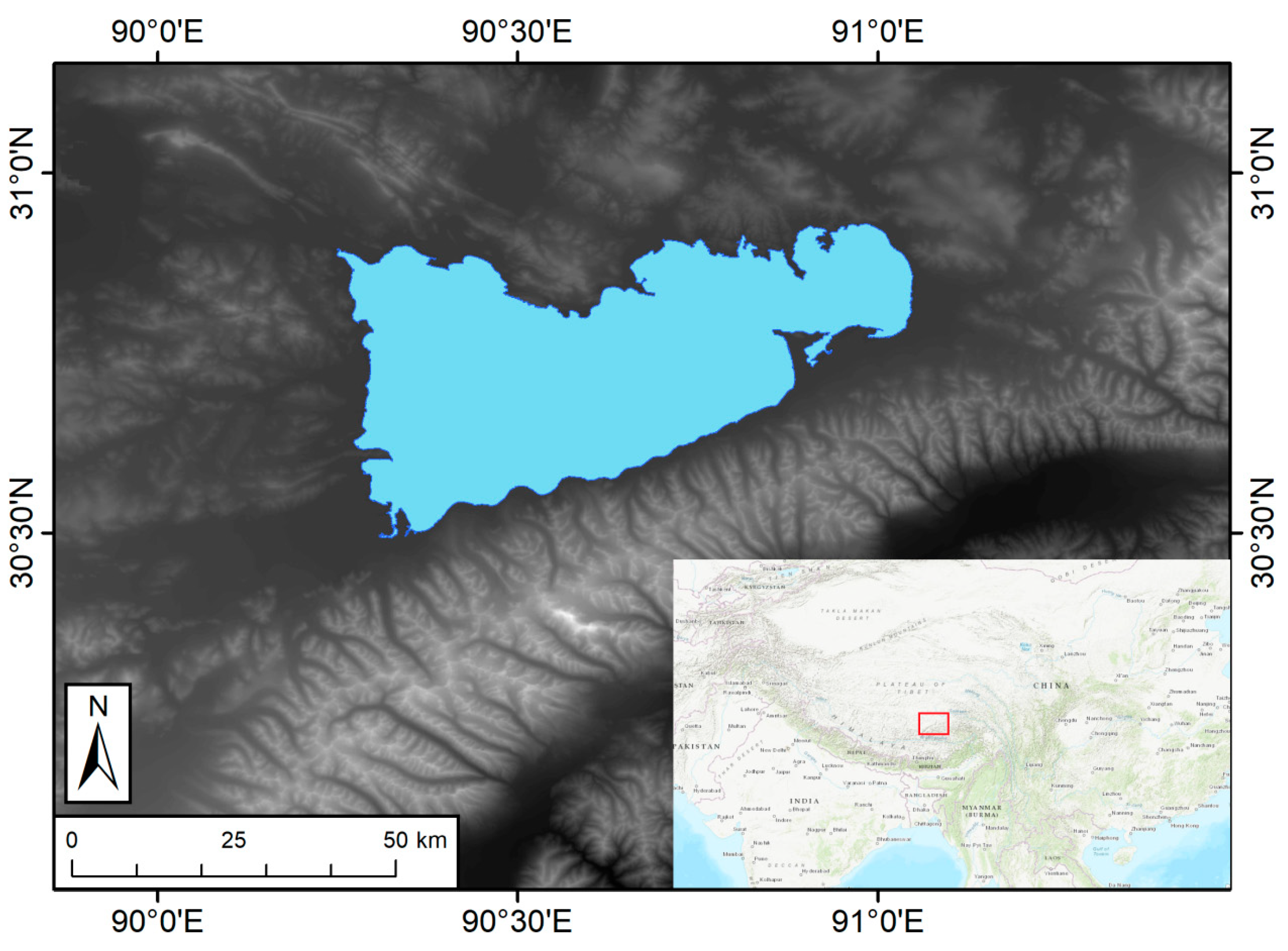
Nam Co is an endorheic, high-altitude lake (4726 m asl) located in the Tibet Autonomous Region of the People’s Republic of China, centered at approximately 30.5°N 90.5°E, with a surface area of around 2000 km2, shown in Figure 1. It serves as the main research focus of the Sino-German “Geoecosystems in transition on the Tibetan Plateau (TransTiP)” project. Its catchment contains a variety of topography, ranging from high-gradient steep relief to flat swamp-like areas. Nam Co is a relatively pristine site, with little human impact and development compared to nearby areas in Asia [3,4] and little vegetation, making its satellite-derived imagery an excellent representation of actual elevation. At the same time, Nam Co remains a fairly data-sparse study site [5,6], making it all the more important to choose an appropriate DEM dataset so as to minimize uncertainty throughout higher-level analyses and modeling. TanDEM-X data at resolutions of 12, 30, and 90 m have recently become available for this region from the German Aerospace Center (DLR) to allow comparisons against the existing publicly available datasets, which all have coverage for the area.
1.2. Datasets
1.2.1. SRTM
The Shuttle Radar Topography Mission (SRTM) was launched in 2000 by the USA National Aeronautics and Space Agency (NASA) in partnership with the DLR and Italian Space Agency, with the intent of developing a near-global DEM based on interferometric data for all latitudes less than 60°, or 80% of land surface on Earth [8]. The system was located on the space shuttle Endeavour and operated between February 11–22, 2000. Datasets of 1 arcsecond and 3 arcseconds are freely available to the public. The generated datasets have postings of 30 m and 90 m at the equator, respectively, height accuracy of 6–10 m, and is based on data from over 180 h of flying time and 180 million square kilometers of land. Absolute and relative height errors for 90% of a large-scale ground-truth campaign’s points were under 10 m for all continents, and absolute geolocation error was under 13 m for all continents, surpassing the respective stated goals of 16 m, 10 m, and 20 m for absolute height, relative height, and absolute geolocation error [9]. Subsequent versions of the original dataset are available with voids from missing data filled in and with a generated water bodies shapefile, as with the 30 m void-filled version 3 we used in our analysis (available from the USGS at https://earthexplorer.usgs.gov/) and the 90 m version 4.1 ([10], available from http://srtm.csi.cgiar.org/).
1.2.2. ACE2
Altimeter Corrected Elevations (ACE) is an effort of the European Space Agency (ESA) to generate a global DEM dataset with 3-arcsecond posting from altimetry data for latitudes between 81.5° N and S and supplemented with ground truth topographic data [11]. ACE2 improves on the original ACE dataset by combining several altimetry datasets from the ERS-1 Geodetic Mission and the EnviSAT RA-2 data with the popular SRTM 90 m data to remove large (thousands of meters) vertical errors found in the original dataset. The highly mountainous areas of the world suffered from poor capture of altimeter echoes, and thus, has large (>16 m) errors. In fact, the Himalaya range had such poor altimeter coverage and results that the original SRTM base data was retained and used alongside altimeter-corrected areas for the rest of the world [11]. We used ACE2 version 1.31 with 90 m posting in our analysis (available from http://tethys.eaprs.cse.dmu.ac.uk/ACE2/).
1.2.3. ASTER
Advanced Spaceborne Thermal Emission and Reflection Radiometer (ASTER) was a joint project between NASA and Japan’s Ministry of Economy, Trade and Industry (METI), who together released the Global Digital Elevation Model (GDEM) in 2009 [12]. NASA spacecraft recorded optical imagery in the form of infrared stereo pairs and then compiled over 1 million of these 60 km x 60 km DEM scenes together into a single dataset. The ASTER GDEM is available at intervals of 1 arcsecond for latitudes less than 83°, thus encompassing approximately 99% of Earth’s land mass, with a reported 95% of measurements having vertical accuracy within 20 m. A second updated version released in 2011 improved this vertical accuracy to 17 m with additional coverage and water masking; this updated version improved coverage for missing areas, however, sometimes at the cost of adding noise or even additional voids from the removal of noisy spikes. GDEM1’s horizontal resolution, in contrast to its 30 m posting, has been likened to approximately 120 m based on comparisons to higher-resolution DEMs through several studies, with GDEM2 improving that resolution to 72 m [12,13]. ASTER’s accuracy is particularly affected at high latitude, cloudy areas, and over forested and water areas [14]. As of this writing, GDEM1 is no longer publicly available, as the hosting agencies have decided that GDEM2 (available from https://lpdaac.usgs.gov/node/1079) is sufficiently improved over GDEM1 and should be the only one in use.
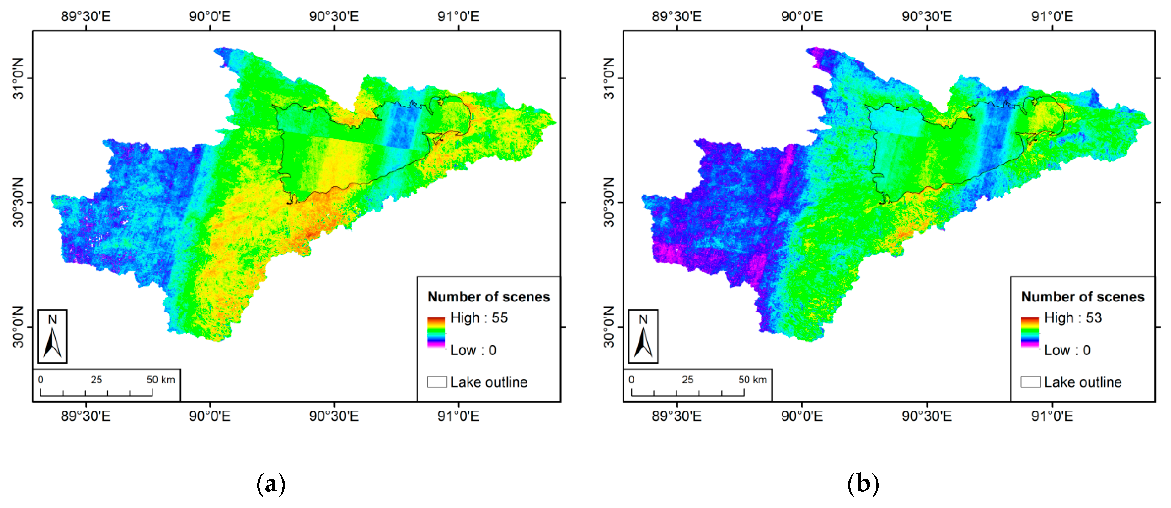
The number of ASTER scenes mosaiced together is used as an indicator of data quality for a given area. The optimal ASTER GDEM measurement at any given point is achieved with between 10–15 scenes [12,15]. Figure 2 shows the ASTER GDEM1 and GDEM2 scenes for the Nam Co catchment. The western regions of the ASTER GDEM1 and GDEM2 datasets have a smaller number of scenes than the other areas, which all have a sufficient number of scenes to display optimal measurements for the region. Thus, these datasets, with the exception of the areas in the west, can be assumed to be the most complete data possible; any errors are associated with errors in the acquisition and processing, not due to a lack of data.
1.2.4. ALOS
The Advanced Land Observing Satellite (ALOS) was launched as a public-private partnership by the Japanese Aerospace Exploration Agency (JAXA) with the Panchromatic Remote-sensing Instrument for Stereo Mapping (PRISM) system in tow, and operated between January 24, 2006, and April 22, 2011. The optical data collected through the use of three radiometers was used to generate the ALOS World3D DEM [16]. The DEM has a resolution of 0.15 arcseconds, or around 5 m, and was resampled to 30 m, which is freely available to the public. The dataset is composed of over three million PRISM DEM scenes, with coverage for latitudes between 80° N and S. Height accuracy to within 5 m based on root-mean-square error (RMSE) (or 9.8 m at 95% confidence level) was achieved through stacking multiple scenes as necessary and through comparison to both SRTM 30 m data and ground-truth points [17]. Included with each DEM data file is a correlation coefficient file, stack numbers, and a mask file. We used version 1.1 for this analysis (available from https://www.eorc.jaxa.jp/ALOS/en/aw3d30/data/index.htm).
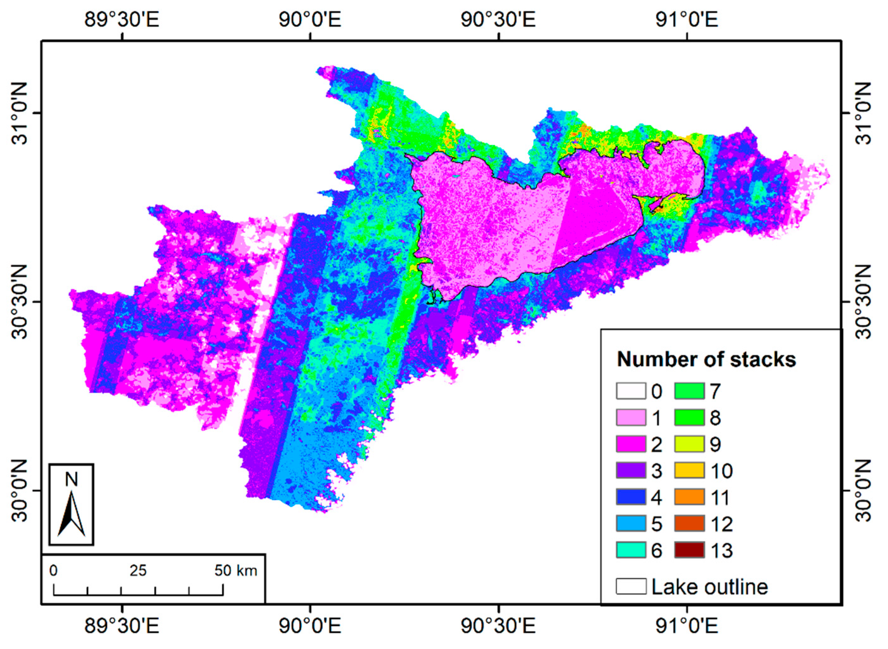
The number of DEM scenes stacked together for Nam Co is shown in Figure 3. The stack number itself is not an indicator of accuracy, though many stacks mosaiced together mean that the underlying area achieved the RMSE goal from that number of stacks. A few areas of this ALOS dataset lack sufficient data, especially in the western and eastern regions with zero stacks listed; those with zero stacks were considered gaps and were subsequently filled in with SRTM 30 m data, as listed in the DEM’s accompanying quality assurance text file. The only section of the ALOS data that was deemed “fair” instead of “good” with regard to integrity (completeness) was over the lake itself.
1.2.5. TanDEM-X
The TanDEM-X (TerraSAR-X add-on for Digital Elevation Models) mission was launched as a public-private effort between the DLR and Airbus Defence & Space, with acquisition dates from December 2010 to January 2015 [18,19]. TanDEM-X uses single-pass interferometry with two X-Band synthetic aperture radar (SAR) acquisitions from concurrently-orbiting satellites to generate a global DEM, with between two and four acquisitions for every point on the globe. Datasets of 0.4 arcseconds (~12 m at the equator) and 1 arcsecond (~30 m) using horizontal datum WGS84 and ellipsoid-based vertical datum WGS84 are available from the DLR at a cost and as part of academic partnerships. Additionally, a worldwide 3 arcsecond (~90 m) dataset has just been released free of charge for use in academic research (available from https://geoservice.dlr.de/web/dataguide/tdm90). The 1 arcsecond and 3 arcsecond datasets were created by resampling the 0.4 arcsecond original dataset. Despite being affected by vegetation and snow cover, the datasets are generally highly accurate: absolute horizontal and vertical accuracy in the original dataset meets the goal of being within 10 m for 90% of all points (with actual average accuracy 2 m) and relative accuracy of 2 m [18]. Numerous studies have examined the dataset’s accuracy across a variety of locations and landscapes, and in most cases, the measured accuracy far exceeds the dataset’s stated goals, with average accuracies ranging from within a few meters to less than a meter [20,21,22,23,24,25,26]. The studies found TanDEM-X data to be better than the next-best alternative such as SRTM, and thus, the best available product short of high-resolution (1 m) DEMs. Due to its accuracy in different settings across the planet, researchers have used the TanDEM-X 12 m dataset as a reference in the absence of ground-truth elevation data [27]; we also employed this technique in our study, using processed results from the TanDEM-X 12 m dataset as a baseline against which to compare results from other datasets. We used 12, 30, and 90 m posting datasets provided by DLR [28].
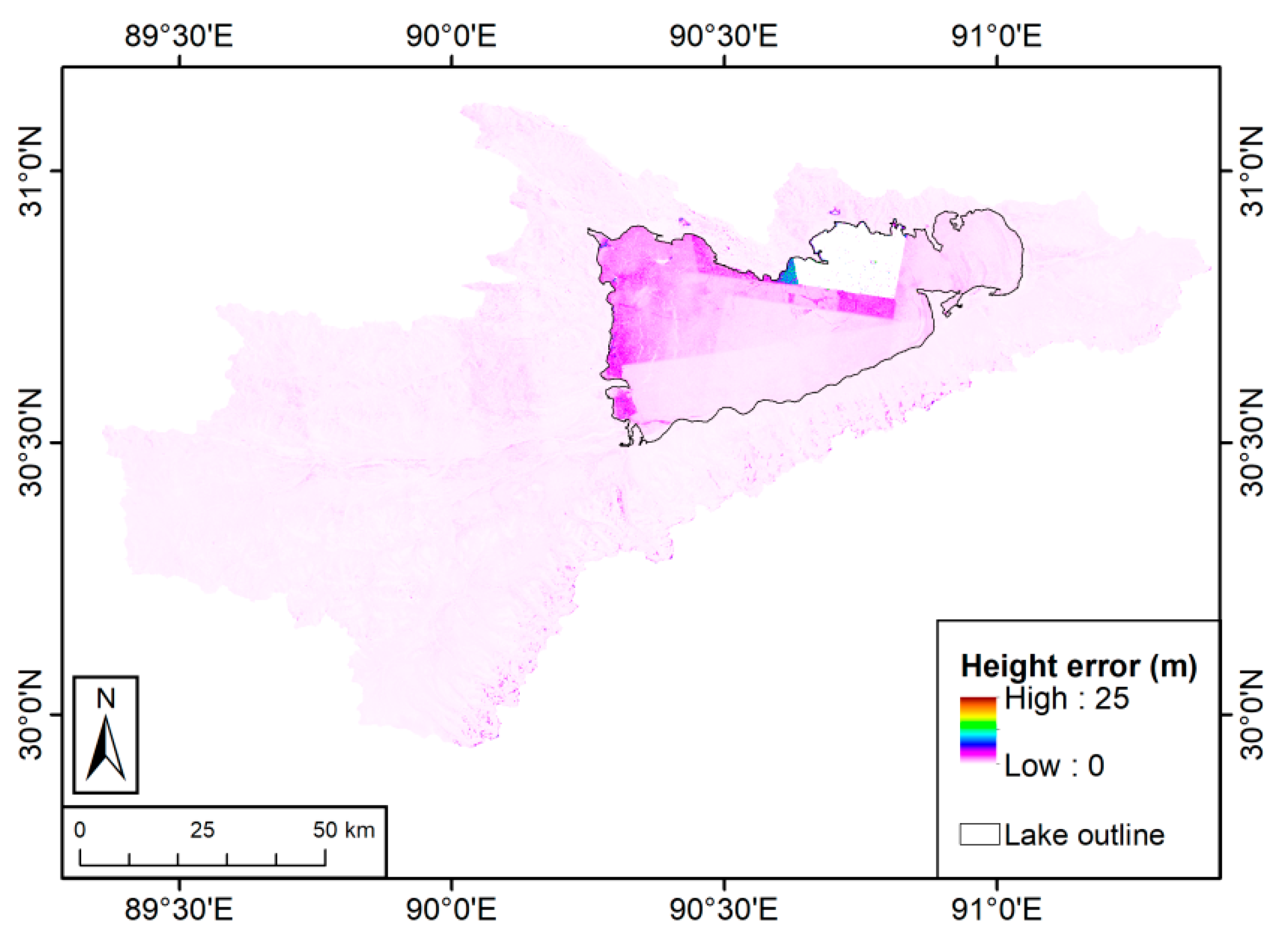
TanDEM-X datasets include several files that can be used to process accuracy and to understand potential data discrepancies: amplitudes, water mask, measurement consistency, height error, coverage, and layover and shadow mask [18]. The mean and minimum amplitudes assist with water detection and allow for crisp coastline development in the mosaicking process. The Height Error Map (HEM) is useful for showing how coherent the data passes are for an area, in essence giving the user an idea of how close to optimal one can expect the data to be. The TanDEM-X height error map for Nam Co, shown in Figure 4, represents random interferometric coherence errors. The error shown here is relatively small, with the highest error values occurring over the lake water areas. The TanDEM-X 12 m dataset has height error <0.5 m for 79.3% of the catchment, <1.5 m error for another 14.7% of the catchment, <2.5 m error for another 2.6% of the catchment, and <9.5 m error for an additional 1.3% of the catchment, meaning that the catchment has an error of <9.5 m for 97.9% of its area; 0.1% of the catchment has error ranging up to 26.7 m located in points associated with water, namely the lake and its edges but also with a few individual points on the glaciers in the southern part of the catchment. An additional 2% of the HEM values were invalid or missing and were mostly located over the lake.
1.3. Related Work
Numerous researchers have addressed quantification and estimation of errors and uncertainties in DEM data largely through comparison to measured, ground-truth datapoints. The question of how cell-by-cell errors affect geomorphometric and hydrologic applications remains more open, though researchers have begun to tackle these specific applications. Only a portion of DEM users take into account the potential errors that DEMs can have on their work [29], thus, it is necessary to examine these potential problems and determine which DEMs are most appropriate for which applications.
Before the ubiquity of high-resolution, high-quality, easily-accessible DEMs, studies focused on particular applications and how their underlying data might affect research outcomes. Hydrological modeling has the potential to be affected not just by the accuracy of vertical data but also by the horizontal resolution of DEMs, as well as by time and space resolution [30,31]; one study noted that 10 m seems to be the best resolution for the tradeoff in accuracy and ease of obtaining data [32], while another suggests selecting a DEM with resolution finer than the hillslope length [2]. Yet another study found that how flowpath is generated (as a single or multiple flowpath) can have a greater impact than DEM scale or other watershed characteristics [33]. Geomorphological parameters ranging from contributing area and fine-grained changes in bar-level topography have the potential to be affected by DEM errors or discrepancies [34,35].
In the 2000s, researchers began to test the accuracy of newly-available DEMs and to compare them to one another in a constant attempt to find the “best” product, often reaching different conclusions. Because both ASTER and SRTM data have been freely available to the public for over a decade and at relatively high resolutions, several studies have compared the results of the two DEM datasets, particularly for geomorphological and hydrological work. These studies generally agree that SRTM is more accurate, but note that both SRTM and ASTER are affected by vegetation [36,37], though SRTM might be less affected due to its ability to penetrate some level of the canopy [15]. Both datasets were found adequate to develop engineering predictions about glacial lake outbursts in Tibet, though ASTER overestimated flood heights [36]. Despite SRTM generally being recognized as having more vertical accuracy, several studies found that ASTER better represented geomorphological properties such as slope gradient and curvature and related landscape forms such as cliff faces and glaciers [38,39]. Studies comparing the accuracy of SRTM, ASTER, and ALOS data have reached mixed conclusions, including that SRTM 30 m and ALOS compared favorably against a Chinese reference DEM [40], that ALOS was the best DEM in the detection of karst in Brazil [41], and that no one DEM produced preferred results for glacial lake outburst modeling [42].
As mentioned earlier, numerous studies have examined and supported the documentation of high horizontal and vertical accuracy of TanDEM-X data, though they differ on recommending TanDEM-X as the ultimate DEM to use in every application. The TanDEM-X 12 m DEM and intermediate DEM were found to be superior to SRTM and ASTER datasets in accuracy and landform identification [20,43,44] and when compared to ALOS in calculating geomorphometric parameters [45]. On the other hand, a comparison of DEMs for geomorphological analysis concluded that TanDEM-X 12 m produced drainage network errors in localized high-relief areas, despite its high vertical accuracy and resolution, and recommended the use of ALOS data based on its accurate drainage network and free availability [46].
2. Methods
Tiles for each dataset were mosaiced together in geographic coordinate system WGS1984 and then projected to the conformal UTM46N projection using bilinear resampling. We geoid-corrected the ellipsoid-based TanDEM-X data using the geoid undulation dataset EGM2008 [47] and the ArcGIS Raster Calculator according to the equation:
where h is the ellipsoidal height contained in the TanDEM-X dataset, H is the geoid-corrected (orthometric) height, and N is the difference between the geoid and reference ellipsoid and contained in the EGM2008 dataset [48]. We used the ArcGIS Warp tool to translate each ACE2 tile from its custom coordinate system (wherein the tile’s coordinates are listed as pixels and range from 0 to 18,000 in both the x and y directions) to the proper coordinates in WGS1984.
h = H + N
Then, for each of the nine datasets, we delineated catchments and subcatchments of Nam Co using the standard workflow of the ArcHydro toolkit in ArcGIS 10.5. We filled sinks in the DEM, generated flow direction using the default D8 algorithm, calculated flow accumulation, and generated stream and drainage networks based on a critical area of 10 km2. This critical area was chosen based on a comparison of generated stream network with those major streams visible on satellite imagery available in Google Earth; 10 km2 was fine-grained enough to generate streams for all those clearly visible in Google Earth. Then, we generated a set of points where drainage lines intersected a minimal TanDEM-X 12 m water mask for the lake and delineated the overall Nam Co catchment and individual subcatchments for each lake intersection point. Lastly, we projected the catchments into the area-preserving Albers Conic projection and calculated the geometry (area) of each subcatchment.
After all catchments and subcatchments were generated and their areas calculated, we used the TanDEM-X 12 m delineations as a basis for comparison against all the other DEM datasets, as it provides the highest geometric resolution and best available dataset. We calculated the centroids of the TanDEM-X 12 m subcatchments and intersected them with the other datasets’ subcatchments in order to pair each respective TanDEM-X 12 m subcatchment with a corresponding subcatchment from each dataset. Then, we exported the intersection data and used R to analyze the differences in area from the TanDEM-X 12 m data. First, we calculated the standard error of the mean (SEM) for the delineated area of each subcatchment i of the 49 subcatchments as the standard deviation divided by the sample size (the number of DEM datasets, N = 9):
σMi = σi/N1/2
Then, we used the Spearman correlation test (rcorr from the Hmisc R library, available at https://CRAN.R-project.org/package = Hmisc) to compare the subcatchment SEM values with the following subcatchment variables from the TanDEM-X 12 m dataset: mean slope, maximum slope, median slope, mean curvature, and area.
In a separate analysis, each DEM dataset was compared individually to TanDEM-X 12 m. We calculated the normalized subcatchment area of each subcatchment i for DEM j using the following equation:
[Normalized area]ij = [subcatchment area]ij/[TanDEM-X 12 m subcatchment area]i
Then, we calculated the Spearman correlation between normalized area and TanDEM-X 12 m subcatchment variables mean slope, maximum slope, median slope, mean curvature, and area.
3. Results
3.1. Catchment Delineations
Table 1 lists the datasets and overall catchment delineation areas, which did not vary largely from the TDX12 data, with the overall mean of all datasets differing by less than 5 km2 from the TDX12 dataset. TDX90 and TDX30 were the closest in size to TDX12, with a difference of less than 1 km2 each, followed by ALOS and SRTM90 with a difference of less than 10 km2. SRTM30 and ACE2 were both approximately 40 km2 smaller than TDX12. ASTER1 and ASTER2 had the largest difference from the TDX12 dataset, respectively 75 and 80 km2 larger than TDX12, though the overall area of the catchment is so large that the mean is still within 0.1% from the TDX12 baseline with a SEM of 0.13% of the baseline.
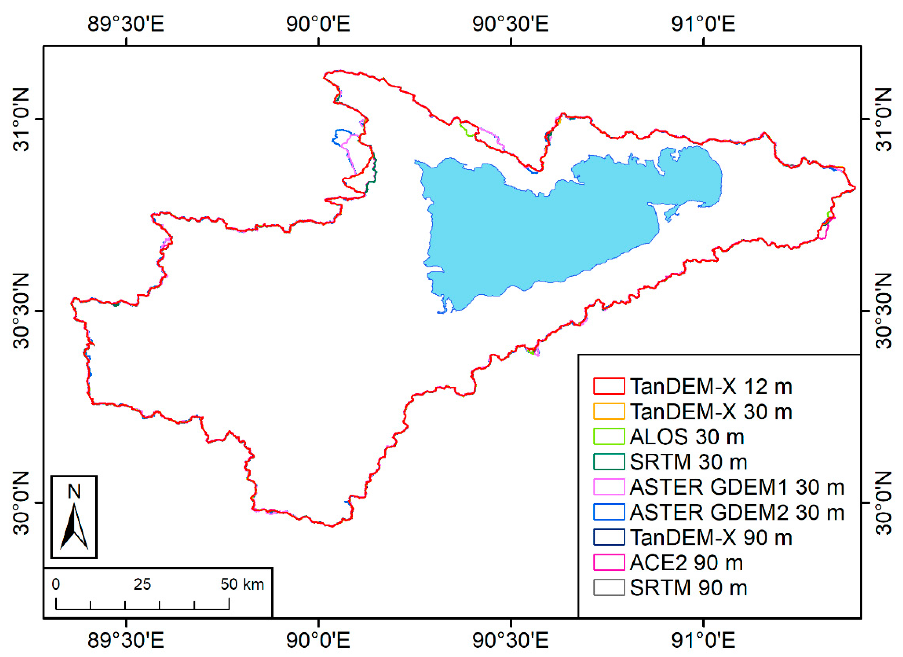
The largest areas of discrepancy were located in the northern area of the catchment characterized by flatter terrain, shown in Figure 5, with each dataset delineating a slightly different boundary and the ASTERs both delineating a noticeably larger area. Across the eastern edge of the catchment all datasets delineated slightly different boundaries but generally agreed for the remainder of the basin with only subtle differences.
3.2. Subcatchment Delineations
Each DEM’s respective subcatchment delineations can be found in Appendix A. Using the centroid intersection method described above, 49 subcatchments from the TDX12 dataset were matched with subcatchments from the remaining eight datasets. Only subcatchments that were contained in all nine datasets were studied using this intersection method. Subcatchment matches were not one-to-one, meaning that some of the underlying datasets had at least one subcatchment that overlaid multiple TDX12 centroids; in particular, the ASTER2 dataset had one large subcatchment in the southwestern area of the catchment that overlaid several smaller, finer-delineated TDX12 subcatchments. Several areas near the shore of the lake did not have a subcatchment covering them due to the chosen minimum area of 10 km2, and thus, no streams appeared in the drainage network or subsequently in the subcatchment delineations.
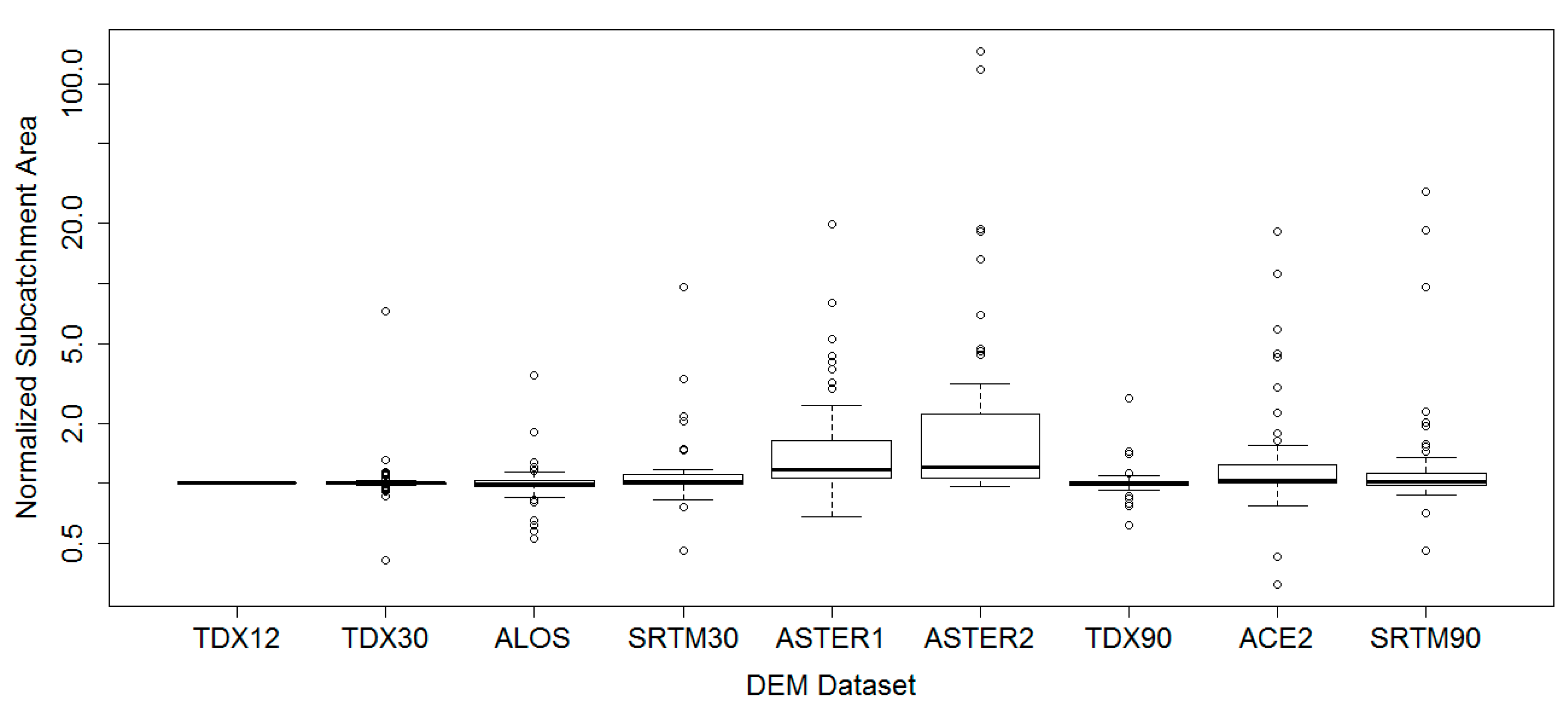
Average differences in delineation area for all 49 subcatchments across the DEM datasets are listed in Table 2. The number of delineated subcatchments varies by dataset, with ACE2 identifying the most subcatchments and ASTER2 delineating the fewest and on average largest. Across the 49 matched-up subcatchments, ALOS, TDX12, TDX90, and TDX30 had the smallest mean delineated areas, followed by SRTM30, then ACE2, ASTER1, and SRTM90, and lastly by ASTER2. It is particularly noteworthy that the resolutions of the DEMs in these groups are not the same, with the least discrepancy in area occurring in both 30 m and 90 m DEMs and the largest discrepancy in area coming from a 30 m DEM. Seven of the DEMs had approximately the same minimum subcatchment area, with the two ASTER datasets having a slightly larger minimum. The TDX12, TDX30, TDX90, and ALOS datasets had notably smaller maximum subcatchment areas than the other datasets. In fact, the SRTM, ACE2, and ASTER datasets had maximum subcatchment areas that were 50% larger than the TDX and ALOS datasets. The TDX90 and ALOS datasets had the closest mean subcatchment area to TDX12 and mean area ratios of 1.03 to TDX12; TDX30 followed closely with a mean ratio of 1.12 to the TDX12 areas. That TDX30 is not the closest match is due to one subcatchment whose larger size in the TDX30 delineation skews the ratio mean, as can be seen in Figure 6. SRTM30 fell on average within a factor of 1.3 of the TDX12 areas, while the ACE2 average ratio was 1.9, SRTM90 and ASTER1 had mean ratios of less than 2.2, and the ASTER2 average ratio to the TDX12 baseline was 7.8. While the ASTER2 mean subcatchment area is approximately three times that of the TDX12 mean subcatchment area, the larger ratio mean between the matched subcatchment areas demonstrates the afore-mentioned matchup of a large subcatchment in ASTER2 with several small ones in the TDX12 dataset on the southwestern side of the catchment. Thus, the larger ASTER2 subcatchments are represented multiple times in ratios with smaller TDX12 subcatchments. The mean values are skewed by the differences in magnitude of these few subcatchments and are merely meant to demonstrate that there are major differences in the delineations produced by the different datasets.
Figure 6 shows the distribution of normalized subcatchment areas by DEM dataset. TDX12, TDX30, TDX90, and ALOS have closely matching median values and tight quartile ranges, despite TDX90’s coarser posting. The SRTM30 and SRTM90 datasets are slightly further from the TDX12 baseline. ACE2 has wider quartiles than the SRTM datasets, and ASTER1 and ASTER2 have much higher median values and wider quartiles than the other datasets. The largest discrepancies can be attributed to a few large subcatchments in the ASTER datasets that the higher-resolution TDX12 split into several small subcatchments, as described previously.
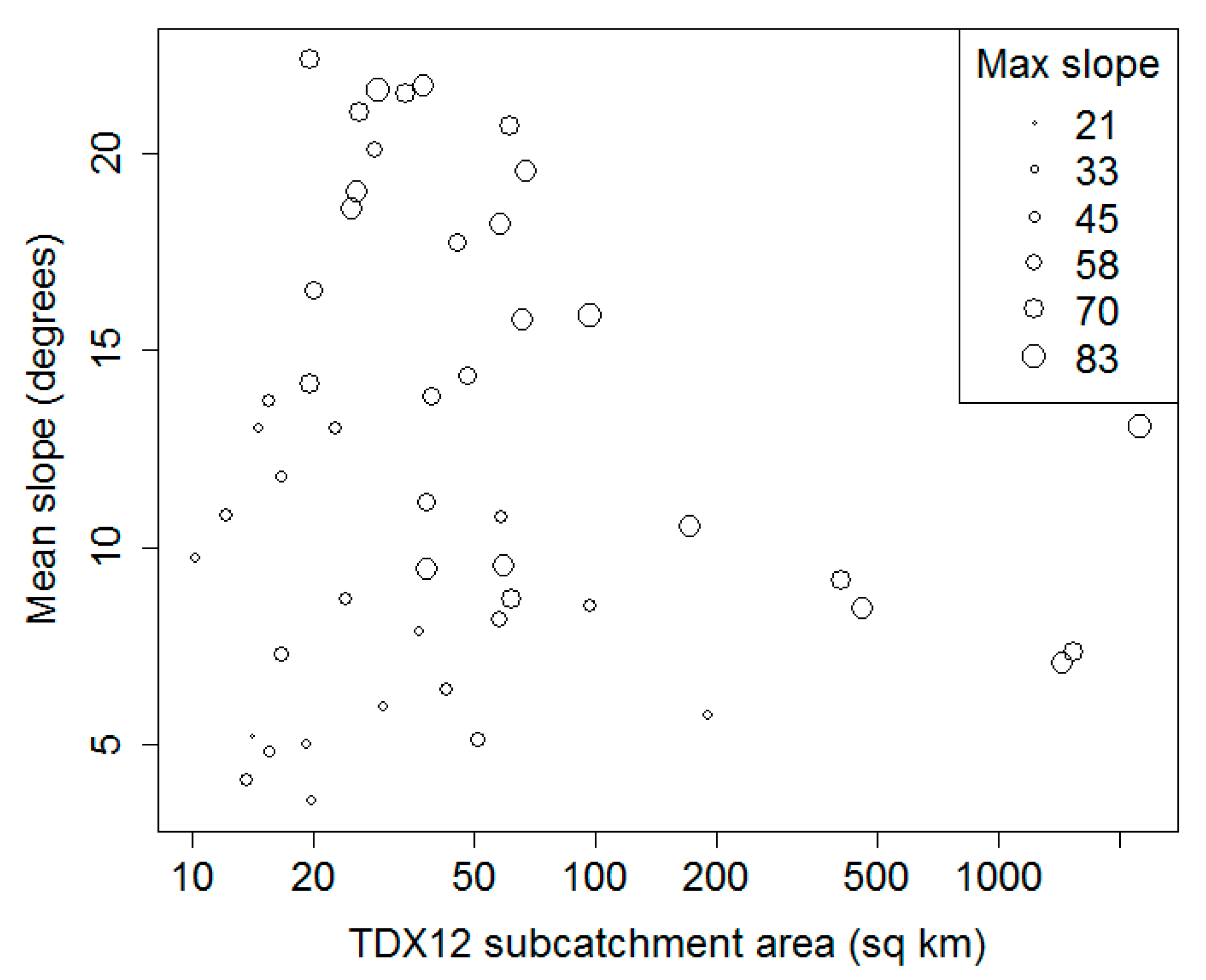
The distribution of TDX12 subcatchment mean slope, max slope, and area is shown in Figure 7. Mean slope covers a range of degrees for smaller subcatchment areas and tends to decrease with catchment size, which matches with Nam Co’s small mountainous subcatchments and larger flatter ones. The maximum slope for each catchment is represented by the point sizes and generally shows higher maximum slopes with higher average slopes, as well as higher maximum slopes for larger catchment areas.
3.3. Error Correlation
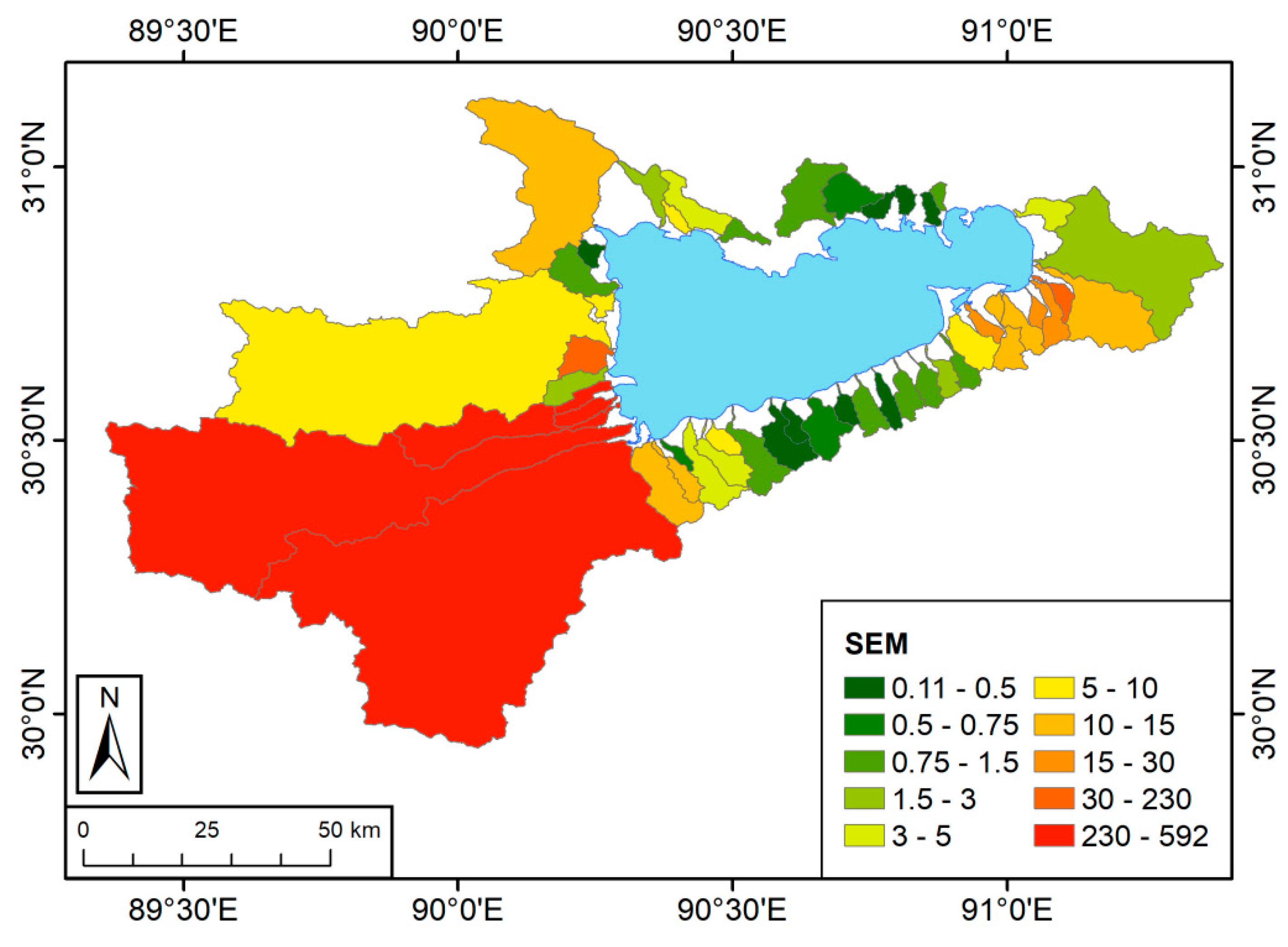
The standard error of the mean (SEM) of subcatchment size, providing a measure of subcatchment delineation uncertainty, is shown in Figure 8. Unclassified, white areas bordering the lake are due to the selected minimum catchment size used to define a stream (see Section 2). Subcatchments along the southern and northern shores of the lake have the lowest error values, while the largest error is located in the western part of the catchment, where the coarser-resolution DEMs delineate large subcatchments that correspond to several small TDX12 subcatchments.
The correlation analysis showed mean and median slope to be significantly but weakly correlated with SEM, with mean slope having a correlation coefficient of −0.29 (p < 0.05), and median slope having a correlation coefficient of −0.34 (p < 0.05).
3.4. Normalized Subcatchment Area Correlation by DEM Dataset
The correlation analysis gives insight into factors that impact a given dataset’s difference from the TDX12 dataset. Only ASTER1 and ASTER2 have normalized area ratios with significant correlations to landscape parameters, with ASTER1 having a negative correlation with subcatchment area of −0.31 (p < 0.05) and ASTER2 having negative correlations with mean, maximum, and median slope values, respectively, of −0.37 (p < 0.01), −0.33 (p < 0.05), and −0.40 (p < 0.005). The remaining datasets do not exhibit any significant correlations between their subcatchment area ratios and the tested environmental variables.
3.5. Outlet Discrepancy Example
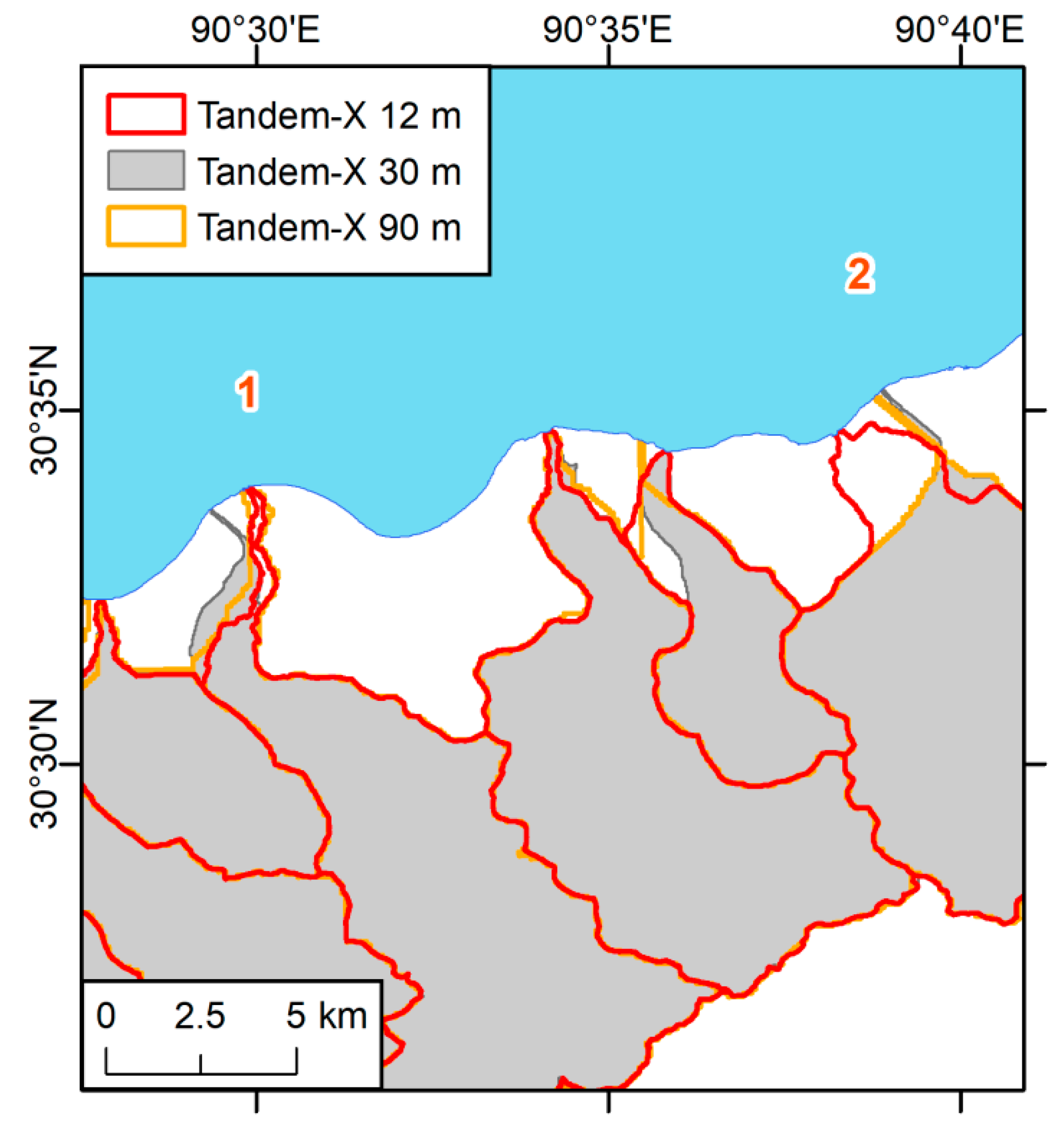
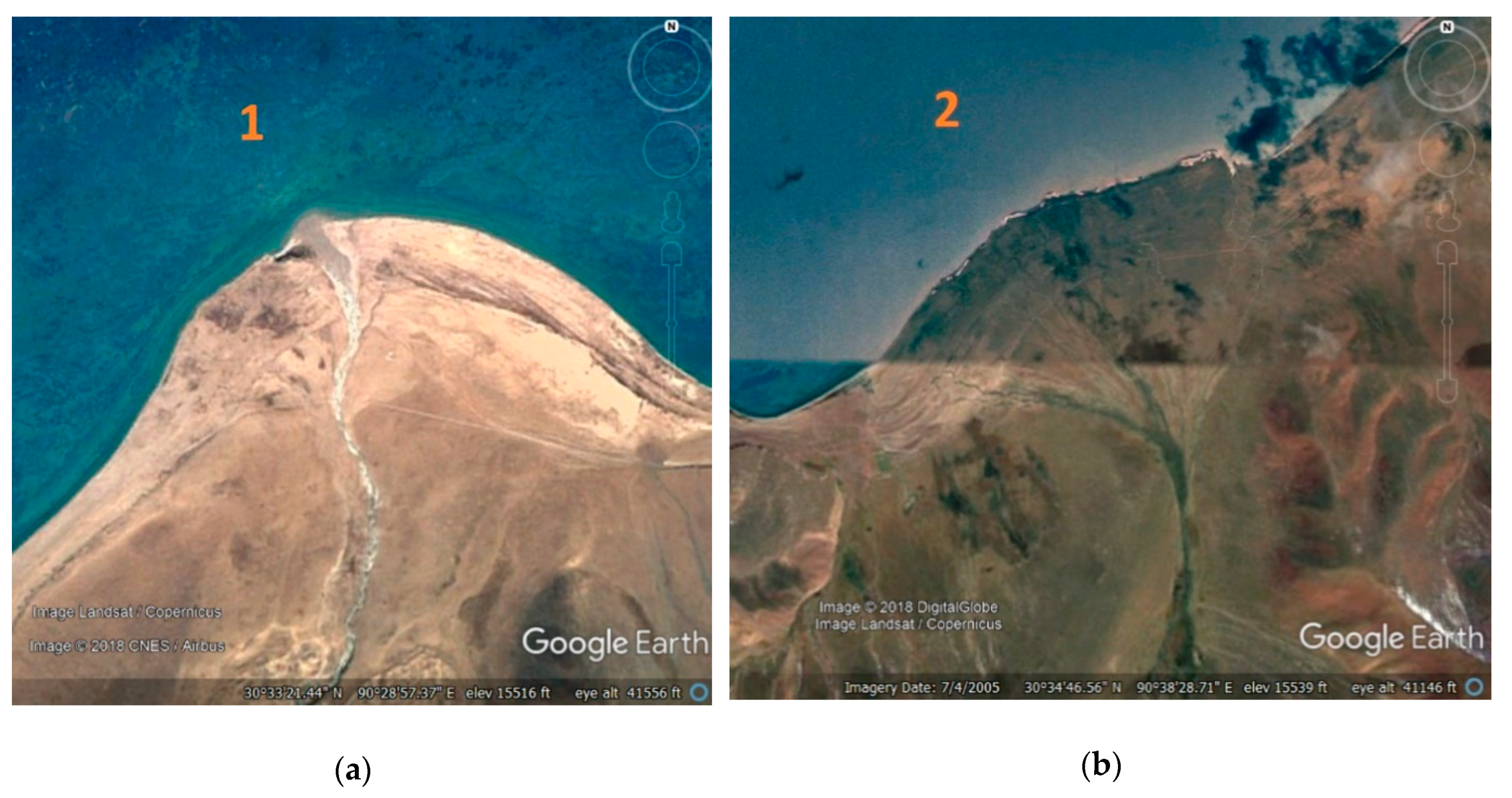
Despite being resampled from the same data, the three TanDEM-X datasets did not always line up perfectly, showing the impact that higher resolution information can have on such details as outlet location and catchment shape. Figure 9 shows two drainage outlets into Nam Co where the TDX12, TDX30, and TDX90 DEMs gave noticeably different outlet points, which in turn affected the remainder of the subcatchment’s shape. While this discrepancy appears to be a serious error at first glance, a closer look at Google Earth imagery for these two subcatchments reveals that these outlets are actually part of alluvial fan features and braided streams. The Google Earth imagery for the two respective outlets is shown in Figure 10. Not all alluvial fan or braided stream outlets exhibit such discrepancies between the two datasets, thus, it is not the case that all geomorphological features of interest can be located based on outlet discrepancies. These points highlight the artefacts associated with the resampling of DEMs.
Hillshade for each of the nine DEM datasets is shown in Figure 11. The TDX12, TDX30, and ALOS datasets are all high-quality enough to see the alluvial fans of the two outlets in question, while these geomorphological features were not apparent in the remaining datasets, despite the apparent crispness of the 30 m datasets. The 90 m datasets were not high-resolution enough to accurately identify the alluvial fans or multiple flowpaths. ASTER1 suffered from artefacts and pits, and while ASTER2 fixed some of these problem areas, the noise (shown as rough texture) in the hillshade images increased the uncertainty in identifying these finer resolution topographical features. SRTM30 seems to be at the tipping point between crispness and noise. The TDX30 and ALOS datasets presented clear imagery, with some water noise present in the ALOS dataset, and the TDX12 data exhibited the exceptional crispness and detail that one would expect from such a high-resolution dataset with a refined process for water detection.
4. Discussion
The overall catchment delineation areas were similar for all the DEM datasets; even the 90 m datasets appear to be good enough for coarse, small-scale analyses. In fact, the TDX90 dataset delineated the area closest to that of its originating dataset, TDX12. The 12 m and 30 m datasets are excellent for finer examination of topography; however, they could be unnecessarily high-resolution for tasks such as delineating 10,000 km2 catchments or, in the case of TanDEM-X, be more difficult to obtain. Supporting a previous study that recommended ALOS due to its more accurate drainage networks and free availability, we found that ALOS gives similar results to the higher quality TDX12 dataset [46]. However, our findings that subcatchment areas were influenced by flatter, less-defined topography also support the idea that TDX12 data’s finer resolution could be better than ALOS for geomorphometric analyses [45]. SRTM, SRTM-based ACE2, and ASTER differed the most markedly from the TDX12 baseline, which is a similar result to studies finding lower accuracy in SRTM and ASTER datasets than in TanDEM-X [20,43,44].
SEM correlation analysis showed that increased errors were somewhat more likely to be found in catchments with lower slopes, which supports the observation of high-slope southern streams having well-defined flowpaths and relatively low error. Flatter areas of subcatchments near the lake tend to have less clearly defined flowpaths, sometimes due to braiding and alluvial fans, and lower resolution DEMs cannot be expected to develop stream networks and catchment delineations on the same scale as higher resolution products in these uncertain areas.
Normalized area correlation analysis showed negative correlation with TDX12 subcatchment area for ASTER1 and negative correlations with mean, median, and maximum slope for ASTER2: smaller TDX12 subcatchments were more likely to have a larger ASTER1 delineation matchup, and flatter subcatchments were more likely to have a larger ASTER2 delineation matchup due to the less defined flowpaths. The negative relationship with slope is the same for both SEM and normalized area analyses: flatter slopes led to less defined flowpaths and differing outlets, which led to different subcatchment boundaries and areas. While these correlations were weak and not definitive, they hint at the role of environmental parameters in error, particularly with the ASTER GDEMs. As such, when working with these DEMs, one should be cautious when working with shallow, low-relief regions and be aware that the DEMs with lower resolution data might overestimate subcatchment areas or miss boundaries between actual subcatchments. The ALOS, SRTM30, TDX30, and TDX90 DEMs showed no such significant correlations, largely because their subcatchment areas did not vary that markedly from the TDX12 areas, and the SRTM90 and ACE2 datasets did not vary markedly with any statistical significance for the tested variables. Posting alone clearly does not capture the whole story with regards to the accuracy of data contained in a DEM, and the environmental parameters tested here do not fully clarify the situation in which a user might encounter greater error. Thus, there is clear evidence of a random error contribution to catchment delineation even in situations where vegetation does not bias a DEM.
Our study focused on the uncertainty induced by the use of different DEMs in the process of catchment delineations. This uncertainty directly transfers into hydrologic modeling results and any kind of derived analyses like the study of erosion and sediment transport by water, restoration schemes in hydrological catchments, and other related studies requiring surface water catchment boundaries. Due to possible random errors in catchment delineation, researchers would be prudent to quantify the uncertainty introduced into their analyses by testing results derived from one DEM with results derived from another DEM.
5. Conclusions
We presented delineations for the semi-arid, high mountain catchment of Nam Co, Tibet and 49 of its subcatchments, based on nine different DEM datasets. The delineated Nam Co catchment areas were very similar, with a mean area that differed by less than 0.1% from the TDX12 dataset and a standard error of 0.13% across all the datasets. These datasets can be approximately grouped by the similarity of their subcatchment results: the TDX12, TDX30, TDX90, ALOS, and SRTM30 datasets delineated similar size subcatchments as compared to the TDX12 baseline; SRTM90, ACE2, and ASTER1 DEMs delineated similar size catchments; and the ASTER2 GDEM delineated subcatchments furthest in size from the corresponding TDX12 subcatchments.
Both lower and higher posting DEMs were able to similarly delineate a large-scale catchment, pointing to the necessity of considering the needs of a given application before deciding on an underlying DEM. While high-posting datasets such as TDX12 have been shown to be highly accurate, the processing needs of such a dataset or barriers to procurement could outweigh a simple application for which the DEM is needed. On the other hand, even datasets of the same posting such as ASTER2 and ALOS can produce drastically different results. This study creates awareness of random error in catchment delineations and shines light on the measures of a landscape that might impact DEM accuracy. Delineations for areas with less clearly defined flowpaths, particularly due to low slopes, produced results that were furthest from the baseline, with the most pronounced differences in older, lower posting DEMs. We caution that these lower-posting, older DEMs such as ASTER and SRTM might provide sufficient coarse-scale results, but could offer drastically different results than newer, improved datasets such as freely-available ALOS and TDX90.
Author Contributions
Conceptualization, J.B.; Formal analysis, L.K.; Funding acquisition, J.B.; Methodology, L.K.; Software, L.K.; Supervision, J.B.; Visualization, L.K.; Writing—original draft, L.K.; Writing—review & editing, J.B.
Funding
This research was funded by the Deutsche Forschungsgemeinschaft (DFG, grant no: GRK 2309/1 - 2018). The APC was partly funded by a voucher from MDPI.
Acknowledgments
The SRTM 30 m data was released by the USGS in September 2014 and the SRTM 90 m data used here is courtesy of CGIAR-CSI. The ACE2 data was provided by the EAPRS Laboratory of De Montfort University. ASTER GDEM1 and GDEM2 is a product of METI and NASA. The original ALOS World 3D 30 m data are provided by JAXA. The Deutsches Zentrum für Luft- und Raumfahrt (DLR) provided TanDEM-X data under the license agreement DEM_HYDR1727. The corresponding proposal was developed in collaboration with Björn Riedel (Braunschweig) and Christiane Schmullius (Jena). This paper is a contribution to the International Research Training Group (IRTG) TransTiP: Geoecosystems in transition on the Tibetan Plateau under the lead of Antje Schwalb (Braunschweig). Roland Mäusbacher (Jena/Heidelberg) was strongly involved in the conceptualization and acquisition of the related funding.
Conflicts of Interest
The authors declare no conflict of interest. The funders had no role in the design of the study; in the collection, analyses, or interpretation of data; in the writing of the manuscript, or in the decision to publish the results.
Appendix A
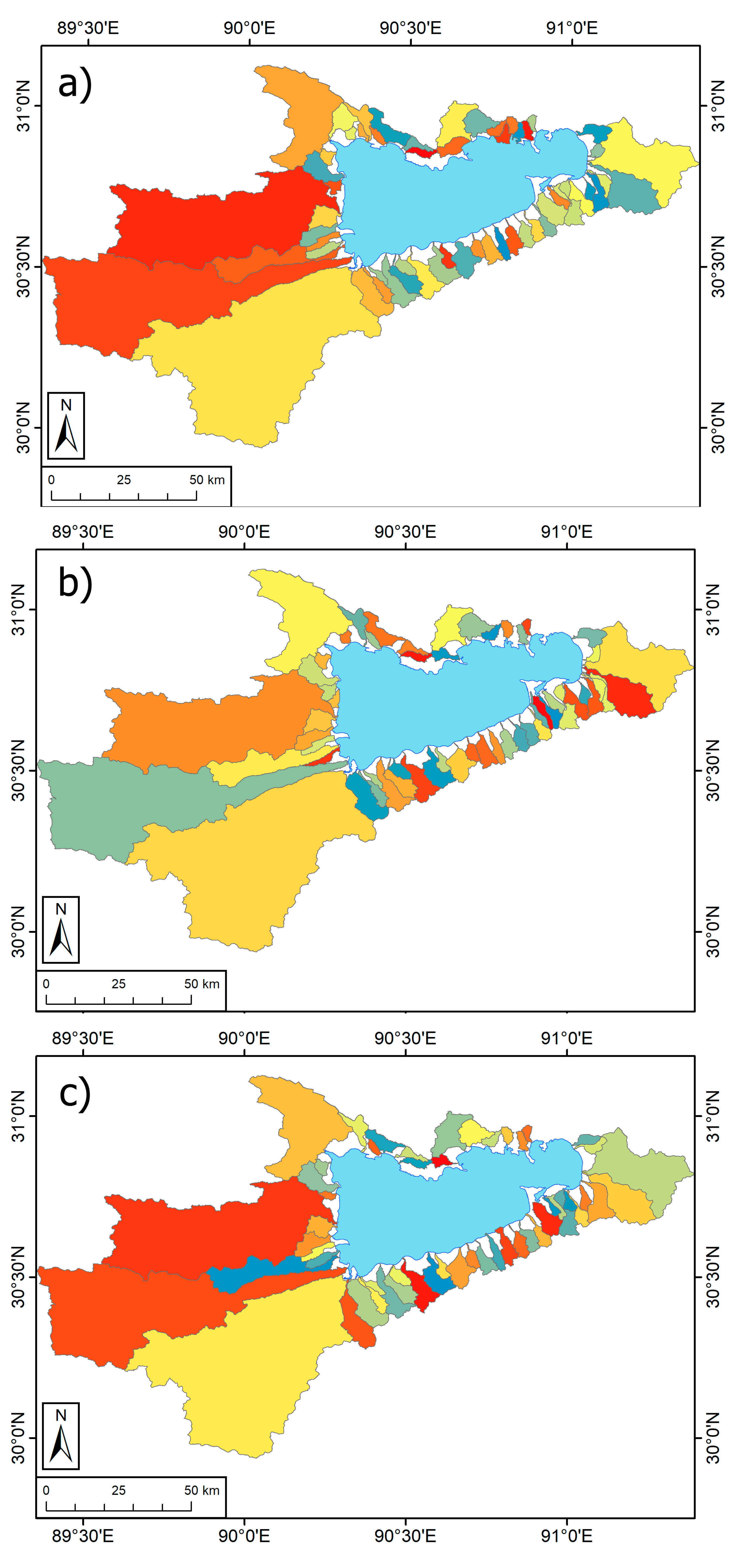
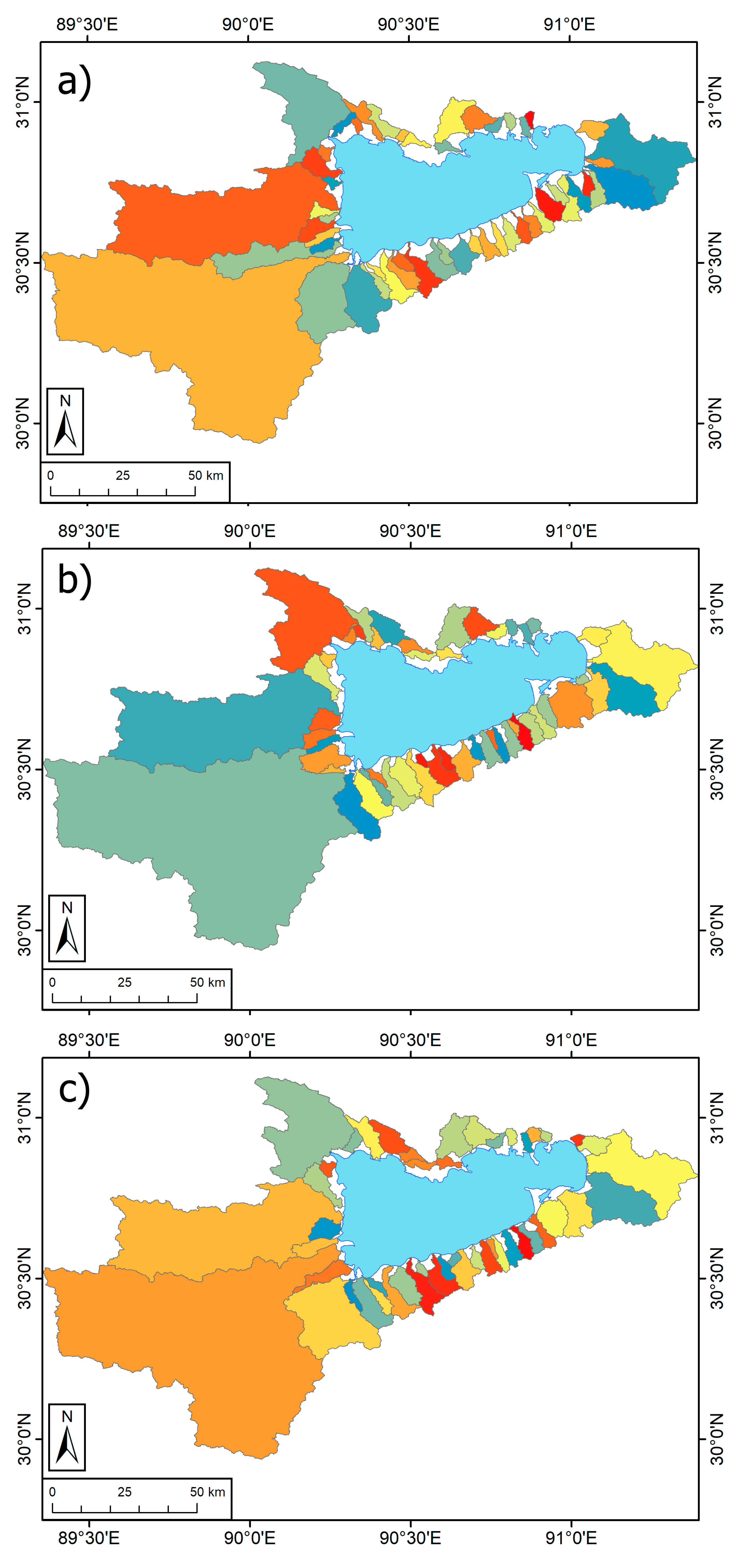
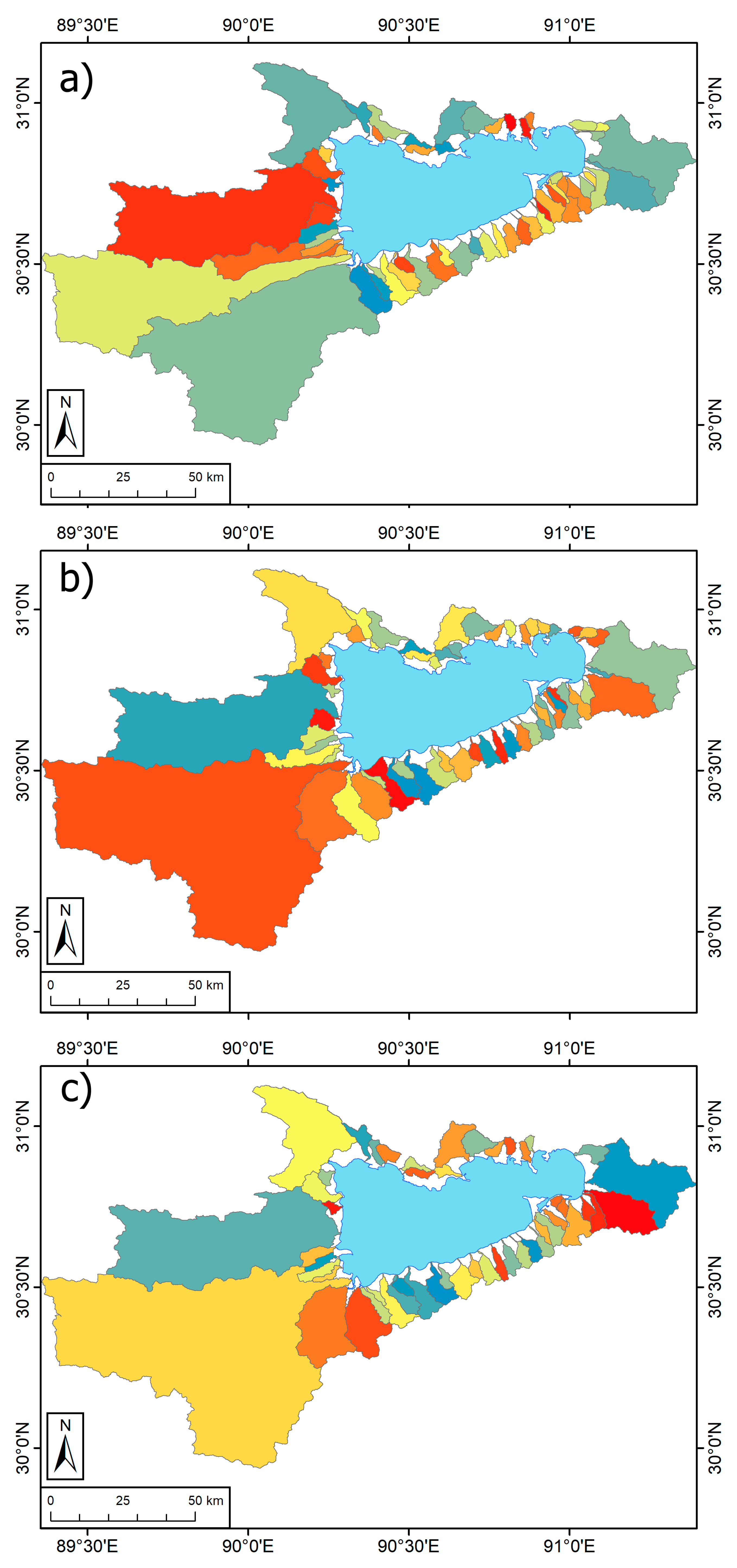
The following subcatchments in Figure A1, Figure A2 and Figure A3 were delineated following the procedure outlined in Section 2, shown here in randomly selected colors and with the lake boundary. Unclassified, white areas bordering the lake are due to the selected minimum catchment size (10 km2) used to define a stream. An estimate of uncertainty is shown in Figure 8 as subcatchment area standard error.
Figure A1.
Subcatchment delineations of (a) TanDEM-X 12 m (b) TanDEM-X 30 m (c) ALOS 30 m.

Figure A2.
Subcatchment delineations of (a) SRTM 30 m (b) ASTER GDEM1 30 m (c) ASTER GDEM2 30 m.

Figure A3.
Subcatchment delineations of (a) TanDEM-X 90 m (b) ACE2 90 m (c) SRTM 90 m.

References
- Smith, M.J.; Pain, C.F. Applications of remote sensing in geomorphology. Prog. Phys. Geogr. 2009, 33, 568–582. [Google Scholar] [CrossRef]
- McMaster, K.J. Effects of digital elevation model resolution on derived stream network positions: EFFECTS OF DIGITAL ELEVATION MODEL RESOLUTION. Water Resour. Res. 2002, 38, 13-1–13-8. [Google Scholar] [CrossRef]
- Huang, X.; Sillanpää, M.; Gjessing, E.T.; Vogt, R.D. Water quality in the Tibetan Plateau: Major ions and trace elements in the headwaters of four major Asian rivers. Sci. Total Environ. 2009, 407, 6242–6254. [Google Scholar] [CrossRef] [PubMed]
- Li, C.; Kang, S.; Zhang, Q.; Kaspari, S. Major ionic composition of precipitation in the Nam Co region, Central Tibetan Plateau. Atmos. Res. 2007, 85, 351–360. [Google Scholar] [CrossRef]
- Biskop, S.; Krause, P.; Helmschrot, J.; Fink, M.; Flügel, W.-A. Assessment of data uncertainty and plausibility over the Nam Co Region, Tibet. Adv. Geosci. 2012, 31, 57–65. [Google Scholar] [CrossRef]
- Krause, P.; Biskop, S.; Helmschrot, J.; Flügel, W.-A.; Kang, S.; Gao, T. Hydrological system analysis and modelling of the Nam Co basin in Tibet. Adv. Geosci. 2010, 27, 29–36. [Google Scholar] [CrossRef]
- ESRI. National Geographic World Map; Accessed 1 November 2018. Using: ArcGIS, Version 10.5; Environmental Systems Research Institute, Inc.: Redlands, CA, USA, 2016. [Google Scholar]
- Werner, M. Shuttle radar topography mission (SRTM): Experience with the X-band SAR interferometer. In Proceedings of the CIE International Conference on Radar Proceedings, Beijing, China, 15–18 October 2001; pp. 634–638. [Google Scholar]
- Rodríguez, E.; Morris, C.S.; Belz, J.E. A Global Assessment of the SRTM Performance. Photogramm. Eng. Remote Sens. 2006, 72, 249–260. [Google Scholar] [CrossRef]
- Jarvis, A.; Reuter, H.I.; Nelson, A.; Guevara, E. Hole-Filled Seamless SRTM Data V4; International Centre for Tropical Agriculture (CIAT): Cali, Colombia, 2008. Available online: http://srtm.csi.cgiar.org (accessed on 2 November 2018).
- Smith, R.G.; Berry, P.A.M. ACE2: Global Digital Elevation Model; EAPRS Laboratory: Leicester, UK, 2010; Available online: http://tethys.eaprs.cse.dmu.ac.uk/ACE2/docs/ACE2_userguide.pdf (accessed on 2 November 2018).
- Meyer, D. ASTER Global Digital Elevation Model Version 2—Summary of Validation Results; ERSDAC, NASA, Earth Resources Observation and Science (EROS) Center: Garretson, SD, USA, 31 August 2011. Available online: https://ssl.jspacesystems.or.jp/ersdac/GDEM/ver2Validation/Summary_GDEM2_validation_report_final.pdf (accessed on 2 November 2018).
- Tachikawa, T.; Kaku, M.; Iwasaki, A. ASTER GDEM Version 2 Validation Report; Earth Remote Sensing Data Analysis Center (ERSDAC): Tokyo, Japan, 12 August 2011. Available online: https://ssl.jspacesystems.or.jp/ersdac/GDEM/ver2Validation/Appendix_A_ERSDAC_GDEM2_validation_report.pdf (accessed on 2 November 2018).
- ASTER GDEM Validation Team. ASTER GDEM Validation Team ASTER Global DEM Validation Summary Report; Earth Remote Sensing Data Analysis Center (ERSDAC): Tokyo, Japan, June 2009. Available online: https://ssl.jspacesystems.or.jp/ersdac/GDEM/E/image/ASTERGDEM_ValidationSummaryReport_Ver1.pdf (accessed on 2 November 2018).
- Gesch, D. Validation of the ASTER Global Digital Elevation Model (GDEM) Version 2 over the Coterminous United States; International Society for Photogrammetry and Remote Sensing: Melbourne, Australia, 2011; pp. 281–286. [Google Scholar]
- Tadono, T.; Ishida, H.; Oda, F.; Naito, S.; Minakawa, K.; Iwamoto, H. Precise Global DEM Generation by ALOS PRISM. ISPRS Ann. Photogramm. Remote Sens. Spat. Inf. Sci. 2014, II-4, 71–76. [Google Scholar] [CrossRef]
- Tadono, T.; Nagai, H.; Ishida, H.; Oda, F.; Naito, S.; Minakawa, K.; Iwamoto, H. Generation of the 30 m-mesh global digital surface model by alos prism. ISPRS Int. Arch. Photogramm. Remote Sens. Spat. Inf. Sci. 2016, XLI-B4, 157–162. [Google Scholar] [CrossRef]
- Wessel, B. TanDEM-X Ground Segment DEM Products Specification Document; DLR (German Aerospace Center), Document: TD-GS-PS-0021, Issue 3.1, 5 August 2016; Earth Observation Center: Weßling, Germany, 2016; Available online: https://elib.dlr.de/108014/1/TD-GS-PS-0021_DEM-Product-Specification_v3.1.pdf (accessed on 2 November 2018).
- Zink, M.; Bachmann, M.; Brautigam, B.; Fritz, T.; Hajnsek, I.; Moreira, A.; Wessel, B.; Krieger, G. TanDEM-X: The New Global DEM Takes Shape. IEEE Geosci. Remote Sens. Mag. 2014, 2, 8–23. [Google Scholar] [CrossRef]
- Baade, J.; Schmullius, C. TanDEM-X IDEM precision and accuracy assessment based on a large assembly of differential GNSS measurements in Kruger National Park, South Africa. ISPRS J. Photogramm. Remote Sens. 2016, 119, 496–508. [Google Scholar] [CrossRef]
- Erasmi, S.; Rosenbauer, R.; Buchbach, R.; Busche, T.; Rutishauser, S. Evaluating the Quality and Accuracy of TanDEM-X Digital Elevation Models at Archaeological Sites in the Cilician Plain, Turkey. Remote Sens. 2014, 6, 9475–9493. [Google Scholar] [CrossRef]
- González, M.C.; Bräutigam, M.B. Relative Height Accuracy Analysis of TanDEM-X DEM Products. In Proceedings of the European Conference on Synthetic Aperture Radar (EUSAR), Hamburg, Germany, 6–9 June 2016; Volume 11, pp. 1172–1176. [Google Scholar]
- Gruber, A.; Wessel, B.; Huber, M.; Breunig, M.; Wagenbrenner, S.; Roth, A. Quality assessment of first TanDEM-X DEMs for different terrain types. In Proceedings of the European Conference on Synthetic Aperture Radar (EUSAR), Nuernberg, Germany, 23–26 April 2012; Volume 9, pp. 101–104. [Google Scholar]
- Lee, S.-K.; Ryu, J.-H. High-Accuracy Tidal Flat Digital Elevation Model Construction Using TanDEM-X Science Phase Data. IEEE J. Sel. Top. Appl. Earth Obs. Remote Sens. 2017, 10, 2713–2724. [Google Scholar] [CrossRef]
- Wessel, B.; Gruber, A.; Huber, M.; Breunig, M.; Wagenbrenner, S.; Wendleder, A.; Roth, A. Validation of the absolute height accuracy of TanDEM-X DEM for moderate terrain. In 2014 IEEE Geoscience and Remote Sensing Symposium; IEEE: Quebec City, QC, Canada, 2014; pp. 3394–3397. [Google Scholar]
- Woroszkiewicz, M.; Ewiak, I.; Lulkowska, P. Accuracy assessment of TanDEM-X IDEM using airborne LiDAR on the area of Poland. Geod. Cartogr. 2017, 66, 137–148. [Google Scholar] [CrossRef]
- Grohmann, C.H. Evaluation of TanDEM-X DEMs on selected Brazilian sites: Comparison with SRTM, ASTER GDEM and ALOS AW3D30. Remote Sens. Environ. 2018, 212, 121–133. [Google Scholar] [CrossRef]
- Gonzalez, C.; Rizzoli, P.; Martone, M.; Wecklich, C.; Tridon, D.B.; Bachmann, M.; Fritz, T.; Wessel, B.; Krieger, G.; Zink, M. The New Global Digital Elevation Model: TanDEM-X DEM and its Final Performance. In Geophysical Research Abstracts; EGU2017-8978; EGU: Munich, Germany, 2017; Volume 19. [Google Scholar]
- Wechsler, S.P. Perceptions of Digital Elevation Model Uncertainties by DEM Users. URISA J. 2003, 15, 57–64. [Google Scholar]
- Bruneau, P.; Gascuel-Odoux, C.; Robin, P.; Merot, P.; Beven, K. Sensitivity to space and time resolution of a hydrological model using digital elevation data. Hydrol. Process. 1995, 9, 69–81. [Google Scholar] [CrossRef]
- Wolock, D.M.; Price, C.V. Effects of digital elevation model map scale and data resolution on a topography-based watershed model. Water Resour. Res. 1994, 30, 3041–3052. [Google Scholar] [CrossRef]
- Zhang, W.; Montgomery, D.R. Digital elevation model grid size, landscape representation, and hydrologic simulations. Water Resour. Res. 1994, 30, 1019–1028. [Google Scholar] [CrossRef]
- Wolock, D.M.; McCabe, G.J., Jr. Comparison of Single and Multiple Flow Direction Algorithms for Computing Topographic Parameters in TOPMODEL. Water Resour. Res. 1995, 31, 1315–1324. [Google Scholar] [CrossRef]
- Wechsler, S.P.; Kroll, C.N. Quantifying DEM Uncertainty and its Effect on Topographic Parameters. Photogramm. Eng. Remote Sens. 2006, 72, 1081–1090. [Google Scholar] [CrossRef]
- Wheaton, J.M.; Brasington, J.; Darby, S.E.; Sear, D.A. Accounting for uncertainty in DEMs from repeat topographic surveys: Improved sediment budgets. Earth Surf. Process. Landf. 2009. [Google Scholar] [CrossRef]
- Wang, W.; Yang, X.; Yao, T. Evaluation of ASTER GDEM and SRTM and their suitability in hydraulic modelling of a glacial lake outburst flood in southeast Tibet. Hydrol. Process. 2012, 26, 213–225. [Google Scholar] [CrossRef]
- Wong, W.V.C.; Tsuyuki, S.; Ioki, K.; Phua, M.-H. Accuracy assessment of global topographic data (SRTM & ASTER GDEM) in comparison with lidar for tropical montane forest. In Proceedings of the Asian Association on Remote Sensing, Nay Pyi Taw, Myanmar, 27–31 October 2014; p. 6. [Google Scholar]
- Hayakawa, Y.S.; Oguchi, T.; Lin, Z. Comparison of new and existing global digital elevation models: ASTER G-DEM and SRTM-3. Geophys. Res. Lett. 2008, 35. [Google Scholar] [CrossRef]
- Oluić, M. (Ed.) New Strategies for European Remote Sensing. In Proceedings of the 24th Symposium of the European Association of Remote Sensing Laboratories, Dubrovnik, Croatia, 25–27 May 2004; Millpress: Rotterdam, The Netherlands, 2005. ISBN 978-90-5966-003-8. [Google Scholar]
- Hu, Z.; Peng, J.; Hou, Y.; Shan, J. Evaluation of Recently Released Open Global Digital Elevation Models of Hubei, China. Remote Sens. 2017, 9, 262. [Google Scholar] [CrossRef]
- De Carvalho, O.; Guimarães, R.; Montgomery, D.; Gillespie, A.; Trancoso Gomes, R.; de Souza Martins, É.; Silva, N. Karst Depression Detection Using ASTER, ALOS/PRISM and SRTM-Derived Digital Elevation Models in the Bambuí Group, Brazil. Remote Sens. 2013, 6, 330–351. [Google Scholar] [CrossRef]
- Watson, C.S.; Carrivick, J.; Quincey, D. An improved method to represent DEM uncertainty in glacial lake outburst flood propagation using stochastic simulations. J. Hydrol. 2015, 529, 1373–1389. [Google Scholar] [CrossRef]
- Mukul, M.; Srivastava, V.; Jade, S.; Mukul, M. Uncertainties in the Shuttle Radar Topography Mission (SRTM) Heights: Insights from the Indian Himalaya and Peninsula. Sci. Rep. 2017, 7. [Google Scholar] [CrossRef] [PubMed]
- Pipaud, I.; Loibl, D.; Lehmkuhl, F. Evaluation of TanDEM-X elevation data for geomorphological mapping and interpretation in high mountain environments—A case study from SE Tibet, China. Geomorphology 2015, 246, 232–254. [Google Scholar] [CrossRef]
- Purinton, B.; Bookhagen, B. Validation of digital elevation models (DEMs) and comparison of geomorphic metrics on the southern Central Andean Plateau. Earth Surf. Dyn. 2017, 5, 211–237. [Google Scholar] [CrossRef]
- Boulton, S.J.; Stokes, M. Which DEM is best for analyzing fluvial landscape development in mountainous terrains? Geomorphology 2018, 310, 168–187. [Google Scholar] [CrossRef]
- Pavlis, N.K.; Holmes, S.A.; Kenyon, S.C.; Factor, J.K. The development and evaluation of the Earth Gravitational Model 2008 (EGM2008): The EGM2008 Earth Gravitational Model. J. Geophys. Res. Solid Earth 2012, 117, 1–38. [Google Scholar] [CrossRef]
- Johnson, A. Plane and Geodetic Surveying; CRC Press: Boca Raton, FL, USA, 2014; ISBN 978-1-4665-8955-1. [Google Scholar]
- Google Earth Pro, 2018. Nam Co, Tibet. 30°33’21.44”N 90°28’57.37”E. Version 7.3.2; Viewed 1 November 2018; Google LLC: Mountain View, CA, USA, 2018.
Figure 1.
Nam Co lake in Tibet, located in red box in inset lower right image (©ESRI 2018, [7]), shown against TanDEM-X 12 m digital elevation model (DEM) (©DLR 2017). At an elevation of 4726 m and size of 2,000 km2, it is both one of the world’s highest lakes and one of the largest on the Tibetan Plateau.

Figure 2.
Quality Indicator for Nam Co area as number of scenes for: (a) ASTER GDEM1 30 m (©METI & NASA 2009); (b) GDEM2 30 m (©METI & NASA 2011). While the western portion of the catchment has a smaller number of scenes available, all other areas have sufficient coverage to provide optimal ASTER elevation data.

Figure 3.
Quality Indicator as stack number for ALOS 30 m DEM for Nam Co catchment (©EORC & JAXA 2017). All areas with non-zero stack numbers attained a satisfactory RMSE value by stacking that number of scenes together, while areas with zero stacks were filled in with SRTM 30 m data. Only a small strip in the western portion of the catchment and along the easternmost portion of the catchment had to be filled in with SRTM data.

Figure 4.
Quality Indicator as height error in meters of TanDEM-X 12 m DEM for Nam Co (©DLR 2017). The areas of the catchment that exhibit the highest interferometric coherence errors are the lake itself. The DEM has a maximum height error of 26.7 m, though 97.9% of the catchment had an error of <9.5 m. Furthermore, 79.3% of the area had an error of <0.5 m. 2% of the Height Error Map (HEM) values were unknown, invalid, or missing (the white section within the lake).

Figure 5.
Delineations of Nam Co basin from nine different DEM datasets. While the ASTER datasets result in a noticeably larger catchment along the northern boundary of the catchment, all datasets have remarkably good agreement for the remainder of the catchment, with the average catchment size falling within 5 km2 of the TDX12 delineation.

Figure 6.
Subcatchment areas normalized to their matching TDX12 subcatchments, with logarithmic scale on the y-axis, grouped by DEM dataset. The TDX30, TDX90, and ALOS datasets have similar median values and relatively tight quartile values, with SRTM30 and SRTM90 datasets following closely, then ACE2, and lastly with the ASTER1 and ASTER2 datasets having a much larger set of subcatchment areas compared to their matching TDX12 subcatchments.

Figure 7.
Graph of TDX12 area, average slope, and maximum slope for subcatchments. Average slope tends to decrease with larger catchment areas, and maximum slope increases with increased average slope but also with larger catchment areas.
Figure 7.
Graph of TDX12 area, average slope, and maximum slope for subcatchments. Average slope tends to decrease with larger catchment areas, and maximum slope increases with increased average slope but also with larger catchment areas.

Figure 8.
Standard error of the mean (SEM) of each subcatchment based on matched subcatchment areas across nine DEM datasets. The southwestern area has the highest SEM due to larger, more coarsely-delineated subcatchments that are paired up with finer TDX12 subcatchments. Unclassified, white areas bordering the lake are due in part to the selected minimum catchment size used to define a stream.

Figure 9.
Two subcatchments and outlets where TDX12 (red), TDX30 (gray), and TDX90 (orange) outlets largely differ (©DLR 2017 & 2018) as a result of different postings from resampling the same underlying dataset.
Figure 9.
Two subcatchments and outlets where TDX12 (red), TDX30 (gray), and TDX90 (orange) outlets largely differ (©DLR 2017 & 2018) as a result of different postings from resampling the same underlying dataset.

Figure 10.
Google Earth imagery of each respective outlet from Figure 9, showing alluvial fans and potential multiple stream paths [49].

Figure 11.
Hillshade DEMs of subcatchments in Figure 9 with lake boundary: (a) TanDEM-X 12 m (©DLR 2017), (b) TanDEM-X 30 m (©DLR 2017), (c) ALOS 30 m (©EORC & JAXA 2017), (d) SRTM 30 m (©NASA & USGS 2014), (e) ASTER GDEM1 (©METI & NASA 2009), (f) ASTER GDEM2 (©METI & NASA 2011), (g) TanDEM-X 90 m (©DLR 2018), (h) ACE 90 m (©De Montfort Expertise Ltd. 2009), and (i) SRTM 90 m (©CGIAR-CSI & Jarvis 2008).


Table 1.
Full catchment delineation area and difference from TDX 12 m baseline. All delineated catchments areas are so close to the TDX12 baseline that the average is a mere 5 km2 different for a more than 10,000 km2 catchment.
Table 1.
Full catchment delineation area and difference from TDX 12 m baseline. All delineated catchments areas are so close to the TDX12 baseline that the average is a mere 5 km2 different for a more than 10,000 km2 catchment.
| DEM Dataset | Abbreviation | Area (km2) | Difference from TDX12 (km2) |
|---|---|---|---|
| TanDEM-X 12m | TDX12 | 10752.35 | 0 |
| TanDEM-X 30m | TDX30 | 10751.71 | −0.64 |
| ALOS 30m | ALOS | 10740.80 | −8.88 |
| SRTM 30m | SRTM30 | 10710.59 | −39.08 |
| ASTER GDEM1 30m | ASTER1 | 10824.83 | 75.16 |
| ASTER GDEM2 30m | ASTER2 | 10830.46 | 80.78 |
| TanDEM-X 90 m | TDX90 | 10752.23 | −0.12 |
| ACE2 90m | ACE2 | 10710.79 | −38.88 |
| SRTM 90m | SRTM90 | 10740.03 | −9.65 |
| Overall mean | 10757.09 | ||
| Standard error | 14.39 |
Table 2.
Number of subcatchments, mean subcatchment areas, min and max areas, and mean subcatchment areas normalized to the underlying TDX12 subcatchment (area ratios). The TDX12, TDX30, TDX90, and ALOS datasets exhibit similar characteristics, followed by SRTM30, then by ASTER1, ACE2, and SRTM90. ASTER2 is an outlier, with fewer subcatchments that averaged much larger than their corresponding TDX12 subcatchments.
| DEM Dataset | Number Delineated Subcatchments | Mean Subcatchment Area (km2) | Min Area (km2) | Max Area (km2) | Mean of Normalized Areas |
|---|---|---|---|---|---|
| TDX12 | 58 | 162.98 | 10.26 | 2248.29 | 1 |
| TDX30 | 57 | 166.95 | 10.19 | 2249.30 | 1.12 |
| ALOS | 54 | 162.06 | 10.09 | 2162.73 | 1.03 |
| SRTM30 | 53 | 228.66 | 10.92 | 3339.39 | 1.29 |
| ASTER1 | 51 | 331.30 | 14.68 | 3772.62 | 2.09 |
| ASTER2 | 48 | 468.30 | 14.91 | 3503.58 | 7.89 |
| TDX90 | 57 | 164.31 | 10.49 | 2251.72 | 1.03 |
| ACE2 | 59 | 308.67 | 11.99 | 3472.71 | 1.90 |
| SRTM90 | 51 | 335.30 | 10.02 | 3519.72 | 2.20 |
© 2019 by the authors. Licensee MDPI, Basel, Switzerland. This article is an open access article distributed under the terms and conditions of the Creative Commons Attribution (CC BY) license (http://creativecommons.org/licenses/by/4.0/).
Share and Cite
MDPI and ACS Style
Keys, L.; Baade, J. Uncertainty in Catchment Delineations as a Result of Digital Elevation Model Choice. Hydrology 2019, 6, 13. https://0-doi-org.brum.beds.ac.uk/10.3390/hydrology6010013
AMA Style
Keys L, Baade J. Uncertainty in Catchment Delineations as a Result of Digital Elevation Model Choice. Hydrology. 2019; 6(1):13. https://0-doi-org.brum.beds.ac.uk/10.3390/hydrology6010013
Chicago/Turabian StyleKeys, Laura, and Jussi Baade. 2019. "Uncertainty in Catchment Delineations as a Result of Digital Elevation Model Choice" Hydrology 6, no. 1: 13. https://0-doi-org.brum.beds.ac.uk/10.3390/hydrology6010013
Note that from the first issue of 2016, this journal uses article numbers instead of page numbers. See further details here.