Modelling Actual Evapotranspiration Seasonal Variability by Meteorological Data-Based Models


1
Department of Civil Engineering, University of Salerno, 84084 Fisciano, Italy
2
Agrosphere Institute (IBG-3), Institute of Bio- and Geosciences of the Research Center Jülich, 52425 Jülich, Germany
*
Author to whom correspondence should be addressed.
Hydrology 2020, 7(3), 50; https://0-doi-org.brum.beds.ac.uk/10.3390/hydrology7030050
Submission received: 15 June 2020
/
Revised: 27 July 2020
/
Accepted: 30 July 2020
/
Published: 2 August 2020
(This article belongs to the Special Issue Soil Water Balance)
Abstract
:This study aims at illustrating a methodology for predicting monthly scale actual evapotranspiration losses only based on meteorological data, which mimics the evapotranspiration intra-annual dynamic. For this purpose, micrometeorological data at the Rollesbroich and Bondone mountain sites, which are energy-limited systems, and the Sister site, a water-limited system, have been analyzed. Based on an observed intra-annual transition between dry and wet states governed by a threshold value of net radiation at each site, an approach that couples meteorological data-based potential evapotranspiration and actual evapotranspiration relationships has been proposed and validated against eddy covariance measurements, and further compared to two well-known actual evapotranspiration prediction models, namely the advection-aridity and the antecedent precipitation index models. The threshold approach improves the intra-annual actual evapotranspiration variability prediction, particularly during the wet state periods, and especially concerning the Sister site, where errors are almost four times smaller compared to the basic models. To further improve the prediction within the dry state periods, a calibration of the Priestley-Taylor advection coefficient was necessary. This led to an error reduction of about 80% in the case of the Sister site, of about 30% in the case of Rollesbroich, and close to 60% in the case of Bondone Mountain. For cases with a lack of measured data of net radiation and soil heat fluxes, which are essential for the implementation of the models, an application derived from empirical relationships is discussed. In addition, the study assessed whether this variation from meteorological data worsened the prediction performances of the models.
1. Introduction
Evapotranspiration (ET) is a major component in the water balance of hydrological systems [1,2]. It is a critical parameter in hydrological applications and uncertainties in its assessment propagate through the hydrological soil–water balance [3]. Distinctions can be made between potential evapotranspiration (PET) and actual evapotranspiration (AET). Potential evapotranspiration measures the ability of the atmosphere to remove water from the surface through the processes of evaporation and transpiration when no limitation or control on water supply exists. Actual evapotranspiration is the quantity of water actually removed by evaporation and transpiration from a surface if the total amount of water is limited. Long-term ET measurements are complex and costly to obtain and, even if some observational data exist, methods to assess ET fluxes such as the eddy covariance approach, chambers, sap flow systems, and weighing lysimeters, are time-consuming and labour-intensive [4]. For these reasons, over the last decade, many different approaches for indirect ET modeling have been proposed and classified according to the mechanisms they mimic.
The methods for PET estimation can be divided into radiation-based, temperature-based, mass transfer-based, and combination methods [5]. The combination-based methods combine energetic drivers such as net radiation and air temperature with atmospheric drivers including the vapor pressure deficit and the wind speed. According to these methods, the energy balance and aerodynamic processes can be integrated to predict the evaporation fluxes. This class of models has been originally theorized by Penman who developed the first combination equation to calculate potential evapotranspiration from an open water surface [6,7]. Various derivations of the Penman equation have taken place over time, including that suggested by Monteith [8]. The radiation-based approaches mainly depend on the available energy and neglect the contribution of the aerodynamic component. According to these approaches, evapotranspiration could be investigated accounting for the variability of radiation. The Priestley–Taylor (PT) [9] model was among the first to introduce a method attributable to this group. The temperature-based models consider air temperature as representative of the available energy for evapotranspiration, so it becomes a key factor able to substantially influence the ET process. Some of the most well-known models falling within this class are the Hargreaves method [10] and Thornthwaite method [11]. Mass transfer-based models are based on the concept of eddy motion transfer of water vapor from an evaporating surface to the atmosphere. These methods are among the oldest ones and adopt Dalton’s law [12,13].
The methods for calculating AET can be divided into four categories that partially overlap with the ones proposed for PET assessment. The four classes include the surface energy balance approaches, combination models, complementary methods, and radiation-based models [14]. The energy balance approaches consist of solving the energy balance equation at the surface where the evapotranspiration results from the difference between the net radiation to the surface and losses due to the sensible heat flux and ground heat flux. The surface energy fluxes could be estimated by coupling in-situ observations with remote sensing imagery, since the former are generally able to give only localized estimates and are subject to instrument failure. Among these approaches are the Surface Energy Balance System (SEBS) [15], the Surface Energy Balance Index (SEBI) [16], and the Surface Energy Balance Algorithm for Land (SEBAL) [17]. The combination-based methods for AET estimates derive from the Penman model. Although it was originally used to predict potential evapotranspiration, adaptations of this model for prediction of actual evapotranspiration have been introduced in the scientific literature and among these the PM1 and PM2 (Penman-Monteith 1 and Penman-Monteith 2) models [18] or MPM (modified Penman-Monteith) model [19] can be listed. The radiation-based methods include a number of models resulting from the PT model. It has been modified over time by several authors who developed advanced formulations of this model in order to translate the Priestley–Taylor estimates of PET into AET rates. Some adaptations of the Priestley–Taylor model include the PT-JPL (PT-Jet Propulsion Laboratory) model [20], the MPT (modified-PT) model [21], and the API (Antecedent Precipitation Index) model [22]. The complementary approaches [23] are based on the complementary feedback between actual and potential evaporation. According to this mechanism, when limited water availability dries the ambient air, AET decreases and the energy that would have been consumed by actual evapotranspiration becomes sensible heat. This warms the atmospheric boundary layer resulting in an increase in PET. A number of different models based on the complementary relationship (CR) have been developed, including the advection-aridity (AA) model [24,25,26], the Granger and Gray (GG) model [27,28], the CRAE model [29,30], and the modified advection-aridity (MAA) model [31,32].
The change in evapotranspiration rates is a result of the limited energy and water availability conditions of the considered areas [33,34,35] since, as said above, actual ET is governed by the amount of available energy while potential ET occurs when the supply of water for this process is non-limiting. Under the Budyko framework, AET is dominated by either precipitation (P) or potential evapotranspiration (PET). AET rates approach precipitation values in the case of a dry climate (i.e., limited water availability conditions), and potential evapotranspiration values are instead similar to precipitation values in the case of a wet climate (i.e., energy-limited conditions). Beyond a long-term characterization, the dry and wet climate conditions can also alternate within the year, resulting in intra-annual ET variability. However, in many situations, the transition between water- and energy-limited conditions is not clear, and there is still a need in the relevant literature to find feasible ways to define the water and energy states in order to capture and properly model the dynamics of evapotranspiration [36]. As water- and energy-limited systems respond differently to climate change, the identification of the transitioning mechanisms is also important to reveal the dynamics of a catchment in response to climate variability [37,38]. Additionally, it should be taken into account that the mechanism of ET variability is quite complex, in particular when the systems are water-limited and, in these cases, particular attention should be payed to the hydrological prediction [35].
The current and recent past specific literature is rich in a large number of approaches which aim at finding the most appropriate method for simulating evapotranspiration fluxes, by comparing predictions from PET and AET models with values of evapotranspiration losses measured from micrometeorological stations. The overall results of the comparative studies, regardless of the number of observational sites (in some instances very large), suggested that there is not a single approach able to outperform other modeling methods for a particular biome [14,20,39,40]).
Within this context, three datasets of eddy covariance observations at the experimental sites of Rollesbroich (Germany), Sister (Oregon), and Bondone mountain (Italy) have been collected and investigated with the aim to provide an effective approach for the prediction of the intra-annual ET variability through the use of different model to represent different periods of the year (wet and dry state periods) without claiming to find very general rules for specific biomes for the ET assessment. The experimental sites, belonging to the TERENO (http://teodoor.icg.kfa-juelich.de/overview-en) and FLUXNET (http://fluxnet.fluxdata.org/) global platforms, feature different climate conditions (temperate Oceanic and Mediterranean) and vegetation covers (grassland and forest), and they result in systems with different limiting factors (energy-limited and water-limited systems). In a first step, a comparison between potential evapotranspiration (modelled by using Penman equation) and actual evapotranspiration, indirectly derived by eddy covariance data, has been performed for the case studies in order to detect when the one approaches the other and, consequently, to characterize the intra-annual ET dynamics. The net radiation has been identified as the meteorological variable able to predict the transition between dry and wet periods and between dominant evapotranspiration mechanisms (AET and PET). In a second step, also based on the findings related to the transition mechanism between potential and actual evapotranspiration, a monthly scale assessment of meteorological data-based models to predict ET has been proposed. Penman formulation has been considered for the assessment of potential evapotranspiration, while the AA and API models have been selected among actual evapotranspiration approaches. The choice of these models has been driven by a number of reasons, among which are the low computational effort in their application, the use of only meteorological data as input variables, the reliability in prediction, and the consolidated use in the scientific literature. The AA and the API methods have been evaluated and compared to a third proposed approach, named a threshold approach, which couples the AET and PET modelling, according to the seasonal ET dynamics. In addition, a calibration of the AET models has also been reported in order to improve the prediction during the dry periods. The calibration doesn’t aim at offering the possibility for a modelling approach generalization, since the present work is not focused on finding a very general rules to be applied for one or the other specific biome, but it seeks to improve the reliability of the seasonal evapotranspiration modelling. Finally, the impact on the threshold model performances of the use of empirical relationships to derive net radiation and soil heat fluxes, if not measured in situ, has been tested.
In summary, taking advantage of a good quality dataset, the current research aims are as follows:
- (i)
- the characterization of the actual evapotranspiration dynamic at the seasonal scale for both energy and water limited systems, by illustrating a methodology able to identify dry (water-limited) and wet (energy-limited) states transition only based on meteorological data;
- (ii)
- explain how embedding the switching between dry and wet dominant states into empirical actual evapotranspiration models could lead to an improvement in the wet periods’ prediction of actual evapotranspiration, especially in the case of water availability limited sites.
- (iii)
- the assessment of the model errors due to the use of empirically-estimated input variables.
2. Materials and Methods
2.1. Sites and Data Description
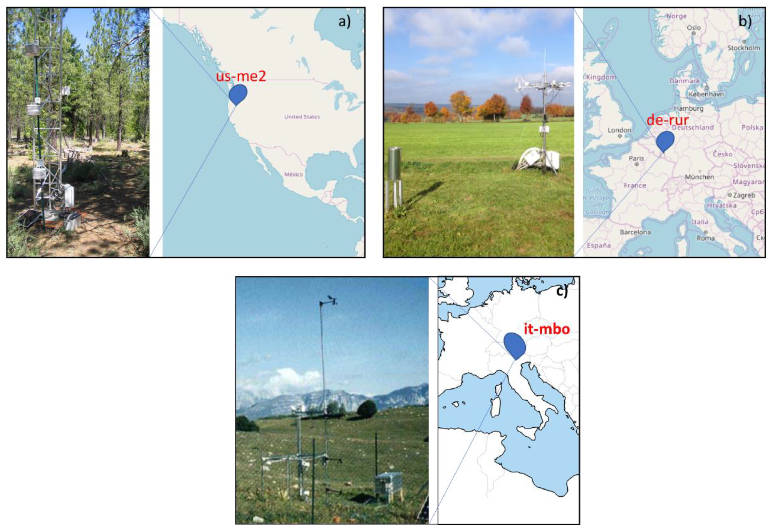
The site “us-me2” (doi:10.18140/FLX/1440079) (Figure 1a) is located near Sister in Central Oregon (4.4523° N, 121.5574° W). The climate is Mediterranean with mean annual precipitation and air temperature, respectively, of 478 mm and 6.9 °C. The observation period used for the analysis ranges from November 2006 to January 2010. The land biome is almost exclusively composed of ponderosa pine trees (Pinus ponderosa Doug. Ex P. Laws) with a few scattered incense cedars (Calocedrus decurrens Florin). Soils at the site are sandy (69%/24%/7% sand/silt/clay at 0–0.2 m depth and 66%/27%/7% at 0.2–0.5 m depth, and 54%/35%/11% at 0.5–1.0 m depth). According to the literature, the rooting depth (RD) for this king of tree is about 1.2 m while the available water storage capacity (AWSC) of predominantly sandy soil is 83 mm/m [41], resulting in a soil water storage (SWS) of 99.6 mm. Within the site, eddy-covariance measurements have been collected using a three-dimensional sonic anemometer and an open-path infrared gas analyzer, additional measurements include atmospheric temperature, relative humidity, and precipitation. The data are collected above the canopy at the towertop level of 33 meters. A more detailed description of the site, instrumentation, data collection and prediction of the flux footprint can be found in [42].The grassland test site “de-rur” (doi:10.18140/FLX/1440215) is located in Rollesbroich, Western Germany (Figure 1b), in the low mountain range of the Eifel region (50.6219° N, 6.3041° E). The climate is Oceanic and during the observation period, April 2012 to July 2016, annual mean precipitation and air temperature are approximately 930 mm and 8.4 °C. The vegetation cover is grassland including meadow foxtail (Alopecurus pratensis), perennial rye grass (Lolium perenne), rough meadow grass (Poa trivialis), and common sorrel (Rumex acetosa). Soils are dominated by (stagnic) Cambisols and Stagnosols on Devonian shales with occasional sandstone inclusions that are covered by a periglacial solifluction clay-silt layer. The literature [41,43] suggests a rooting depth of 0.456 m and an available water storage capacity of 200 mm/m for a SWS of 91.2 mm. Within the site, an eddy covariance tower with a sonic anemometer and an infrared gas analyzer, has been installed since 2011 and latent and sensible heat fluxes have been obtained by the EC technique. The data are collected at 2.6 m above the surface. The EC footprint varies strongly over time as shown in [44]. A more detailed description of the site and the measurement facilities is provided in [45]. The site “it-mbo” (doi:10.18140/FLX/1440170) (Figure 1c) is located near Trento, northern Italy (46.01468° N, 11.04583° E). The site is featured by Oceanic climate with mean annual precipitation of 864 mm and a mean air temperature of 5.1 °C. The period of analysis used for the present research extends from January 2003 to January 2008. The vegetation cover type is mainly permanent alpine meadow with Festuca rubra, Nardus stricta and Trifolium. The soil texture is sandy-loam. As suggested by the literature [41,43], RD is about 0.209 m while AWSC is 125 mm/m, with a soil water storage of 26.1 mm. Since August 2002, an EC system was operational. It consists of an open-path infrared gas analyzer and an ultrasonic anemometer; along with EC flux measurements, the main meteorological variables are measured at a height of 2.5 m. Detailed information about this are provided by [46].
The global platforms guarantee quality assessed (QA) and quality controlled (QC) data for each site. The QA/QC procedure consists in a control check over single variables which allow monitoring of data integrity, correctness, and completeness. In addition, the fluxes from the networks are “energy balance corrected”, which means that the original data have been multiplied by an energy balance closure correction factor calculated for each day from the daily averages of the measured Net Radiation, Soil Heat Flux, Latent Heat, and Sensible Heat. Detailed information about the data-processing is available on the websites of the flux networks. The specific sites selection used in the current study appears critical regarding two main points. Firstly, forests (FOR) and grasslands (GRA) represent some of the most widespread vegetation types covering, respectively, about 40% and 30% of land area in the world [47,48]. Secondly, even though located at almost the same latitudes, the sites substantially differ in terms of climate regimes. In the Mediterranean climate, a clear seasonal cycle with maximum rainfall in winter and minimum in summer can be found, while in the Oceanic climate zone the precipitation is evenly distributed throughout the year. Additionally, these sites have been preferred to others with similar characteristics since they offer a better data quality standard with longer periods of observation and low frequency in the occurrence of missing data. The data used for the current study are air temperature (°C), relative humidity (%), wind speed (m/s), the total net radiation (Mj m−2 d−1) and the latent heat flux (Wm−2) “LH”. The actual evapotranspiration has been calculated from the latent heat flux using the procedure suggested by FAO [49]:
where AET represents the actual evapotranspiration flux (mm) and λ represents the latent heat of vaporization (MJ kg−1).
Since eddy covariance measurements inevitably include missing data or low-quality data, a standard gap-filling procedure was first applied according to [50]. The used method involves replacing the missing values with the average values, under similar meteorological conditions, within a time-window of ±7 days. As reported in [51,52], the days with a rate of missing data higher than 80% should be excluded by the analysis. Since the data are recorded every 30 min, the rate of missing data per day represents the ratio between the number of measurements with a 30-min time step, collected during the considered day, and the number of 30-min intervals in the same day. The studied sites exhibit percentages of missing data significantly lower than the limits reported in the scientific literature. Indeed, for the whole observation periods, they amount to 5.9% for de-rur, 5.1% for us-me2, and 0.01% for it-mbo. A summary is provided in Table 1.
2.2. Models Selection for Potential and Actual Evapotranspiration Assessment
In the current work, Penman formulation has been considered for the assessment of potential evapotranspiration, while the AA and API models have been selected among actual evapotranspiration empirical relationships. According to the literature, the Penman model, belonging to the category of the combined methods, is the most commonly used method to derive potential evapotranspiration [53], so, it has been selected since it represents a well-consolidated model. The AA and API models respectively belong to the complementary and radiation-based categories. Even if these classes of methods may appear to be an old-fashioned approach, a continuous and rising interest has appeared in their application in the scientific literature [14]. Indeed, they are accessible to less experienced users and require only basic meteorological data, provided, free of charge, by open access archives. In addition, these models are also foreseen for forecasting purposes. They have been proven to predict, with a good accuracy, the variations in evapotranspiration fluxes using the projections of future climate scenarios [54,55,56]. On the contrary, combination-based and energy-balance approaches, although very accurate, require significant computational efforts and technical expertise for their implementation. Moreover, detailed input parameters are needed to run these models. Finally, the AA and API models were proven to result in a very good fit to the observations [57,58,59].
2.2.1. Penman Model
The Penman equation PETPM, used for estimating potential evapotranspiration, can be written as follows:
In this formula, evapotranspiration is calculated by weighing the evaporation rate due to net radiation and the evaporation rate due to mass transfer. In Equation (2), Rn represents the net radiation (MJ m−2 d−1); Gsoil represents the soil heat-flux density at the soil surface (MJ m−2 d−1), measured using SHF (soil heat flux) sensors at the surface; and Δ is the slope of the saturation vapor pressure–temperature curve (kPa °C−1) given by the formula [49]:
where Tmean represents the average temperature between maximum and minimum values during the day (°C), γ represents the psychrometric constant (kPa °C−1), λ represents the latent heat of vaporization (MJ kg−1). EA represents the drying power of the air, which is expressed as [49]
In Equation (4), u represents the wind speed (ms−1), 2.6(1 + 0.54·u) is the wind function, es represents the saturation vapor pressure (kPa), ea represents the vapor pressure (kPa).
2.2.2. AA Model
The Advection-aridity (AA) model is an approach commonly used for the assessment of actual evapotranspiration. It is a complementary relationship (CR) model since it is based on Bouchet’s [23] hypothesis which states that a complementary feedback mechanism exists between actual and potential evapotranspiration. The rationale behind this concept is that, under conditions of constant energy input to a given land surface-atmosphere system, water availability becomes limited and actual evapotranspiration decreases below the potential one. The energy that becomes available due to the reduction of actual ET is used to raise the temperature of the air by means of the sensible heat flux, consequently the air is dried and this results in the increase in potential ET in equal amount of the reduction of AET. In the opposite case (increase in water availability), the reverse process occurs, and actual ET increases as potential one decreases. The evapotranspiration occurring when AET equals PET is referred to as the wet environment evapotranspiration. According to [60], the formulation of AA model is
where α is the PT coefficient set at 1.26.
The equation combines an aerodynamic term with an energy component based on net incoming radiation. In particular, the second term of this model represents the effects of large-scale advection in the mass transfer of water vapor represented by the aerodynamic vapor transfer term EA.
2.2.3. API Model
The second model selected for AET prediction in present analysis is the API model. In [22], the Priestley-Taylor model [9] has been modified for the estimation of non-potential evapotranspiration, resulting in the following equation:
The dimensionless coefficient, αAPI, is expressed as a threshold function of the of soil moisture. As surface soil moisture is not routinely available, API index [61] has been used to mimic soil moisture conditions:
where i represents the considered number of antecedent days, k represents the soil decay constant, and represents the rainfall during day t.
Given a threshold value of the API equal to 20 mm [22,62,63], if the current API value is lower than or equal to the threshold API, then
If the current API value is larger than the threshold API, then
assuming that for an over-saturated system (i.e., API > 20 mm), AET rates are no longer dependent on the soil water content, but they are a constant percentage of PET.
2.3. Net Radiation and Soil Heat-Flux Derived from Empirical Formulas
Where measurements of Rn and Gsoil are not available, these variables can be estimated from empirical relationships suggested by [49]. The net radiation can be derived as the difference between the incoming net shortwave radiation (Rns) and the outgoing net longwave radiation (Rnl):
where:
and
In the previous equations, α is albedo or canopy reflection coefficient; Rs is the incoming solar radiation; σ is the Stefan-Boltzmann constant; Tmax,K and Tmin,K are, respectively, the maximum and minimum absolute temperatures during the 24 h period; Rso is the clear-sky solar radiation; as and bs are regression constants, expressing the fraction of extraterrestrial radiation reaching the earth on overcast days; n is the actual duration of sunshine; N is the maximum possible duration of sunshine or daylight hours; Ra is the extraterrestrial radiation in the hour; Gsc is the solar constant; dr represents the inverse relative Earth–Sun distance; ω1 and ω2, respectively, are the solar time angle at the beginning and end of the period; φ is the latitude; δ is the solar declination; z is the station elevation above sea level.
Soil heat fluxes can be empirically derived as follows:
cs represents the soil heat capacity, Ti is the air temperature at time i, Ti−1 is the air temperature at time i − 1, Δt is the length of time interval, Δz is the effective soil depth.
2.4. Models Evaluation
Modelled AET fluxes are in the following compared to the observed AET fluxes from the EC measurements, for the purpose of model evaluation. The comparison helps to test the ability of the selected models to predict actual evapotranspiration fluxes but, even more importantly, it helps to detect the limitations of each approach for each of the cases study and their relevant properties. A monthly scale fitting analysis has been performed, illustrating the specific findings for the whole period of observation as well as for the wet and dry periods, as later better described. Three goodness-of-fit statistics have been accounted for. The normalized root mean square error (RMSEd) as a measure of error magnitude, the index of agreement (d) as a measure of patterns agreement, and the correlation coefficient (r) as a measure of correlation between modelled and measured variables, are estimated as follows:
where n represents the length of the monthly sample, AETmod,i and AETobs,i, respectively represent the monthly values of the modeled and the observed (i.e., derived from EC fluxes) fluxes, σ is the standard deviation, and cov the covariance function.
3. Modelling Results and Discussion
3.1. Transitioning Between Dry and Wet States: Implication for a Threshold Approach
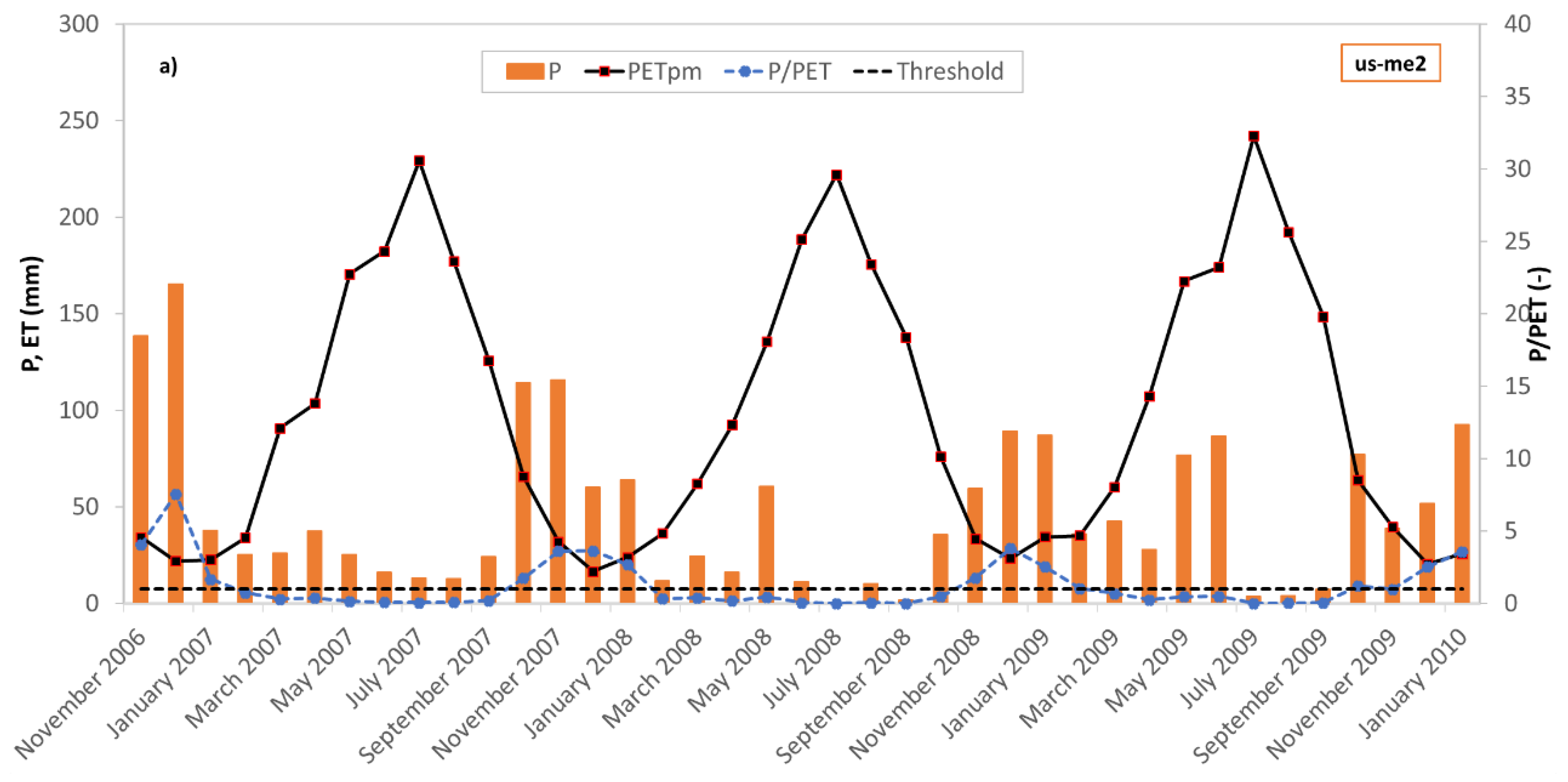
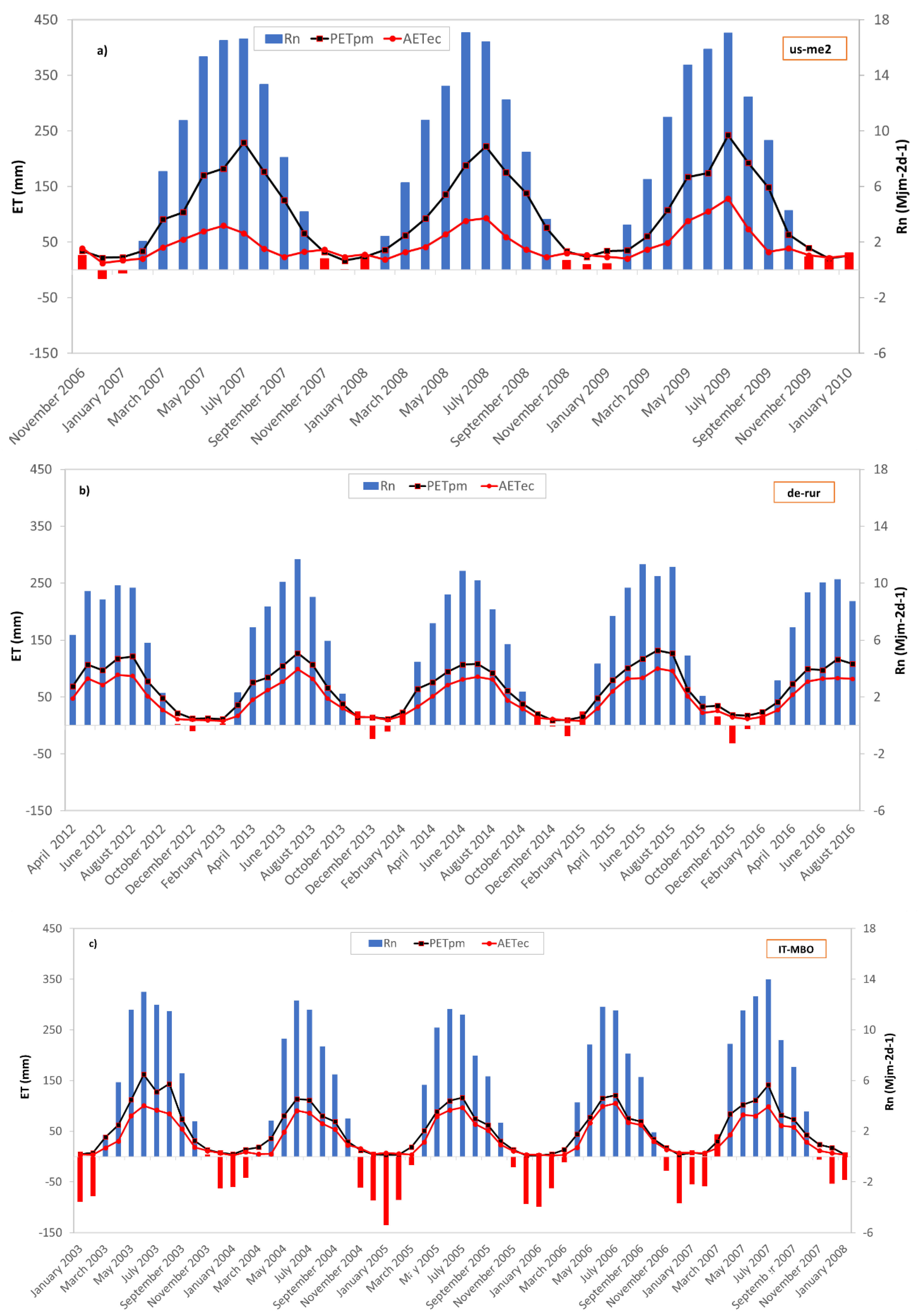
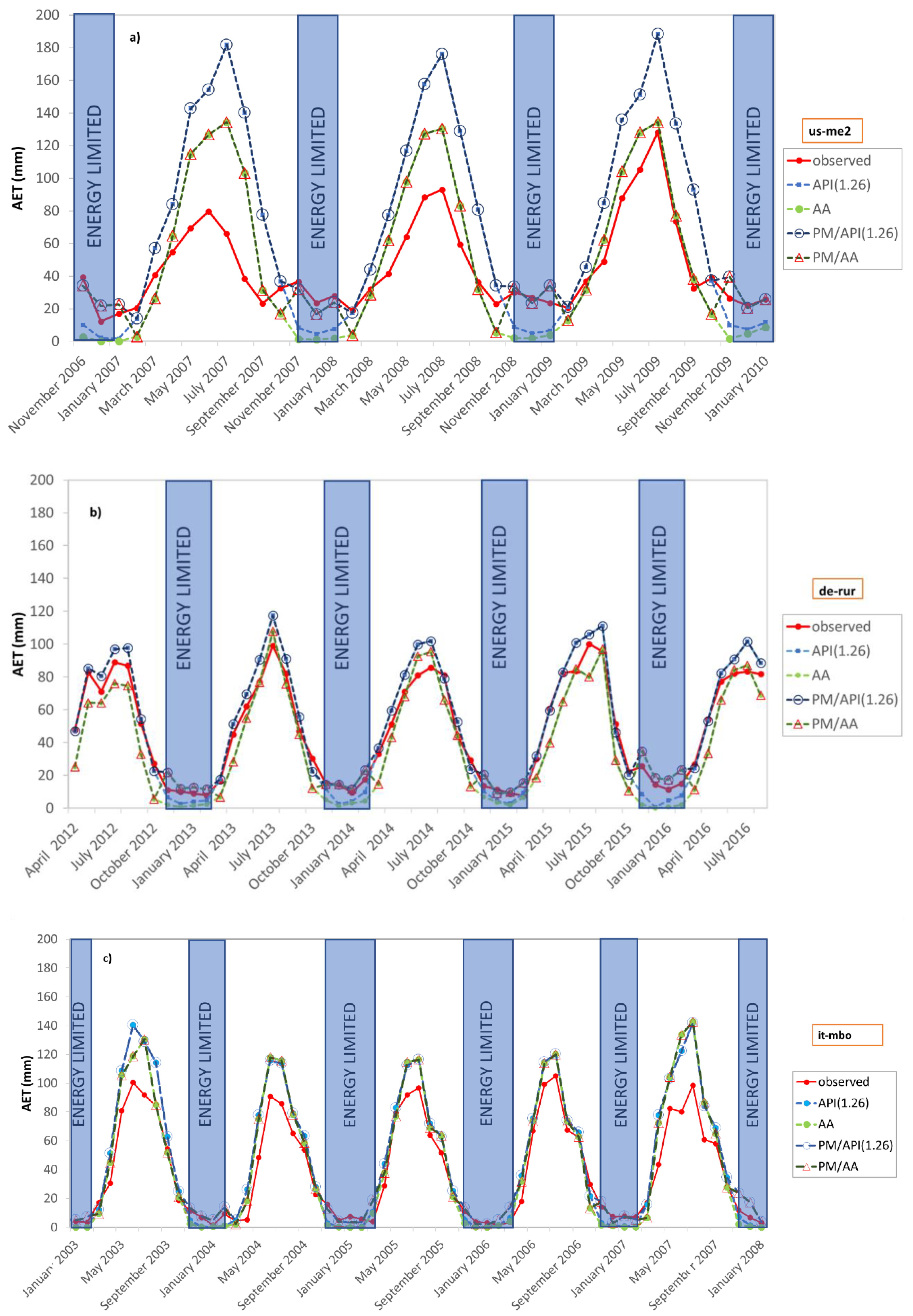
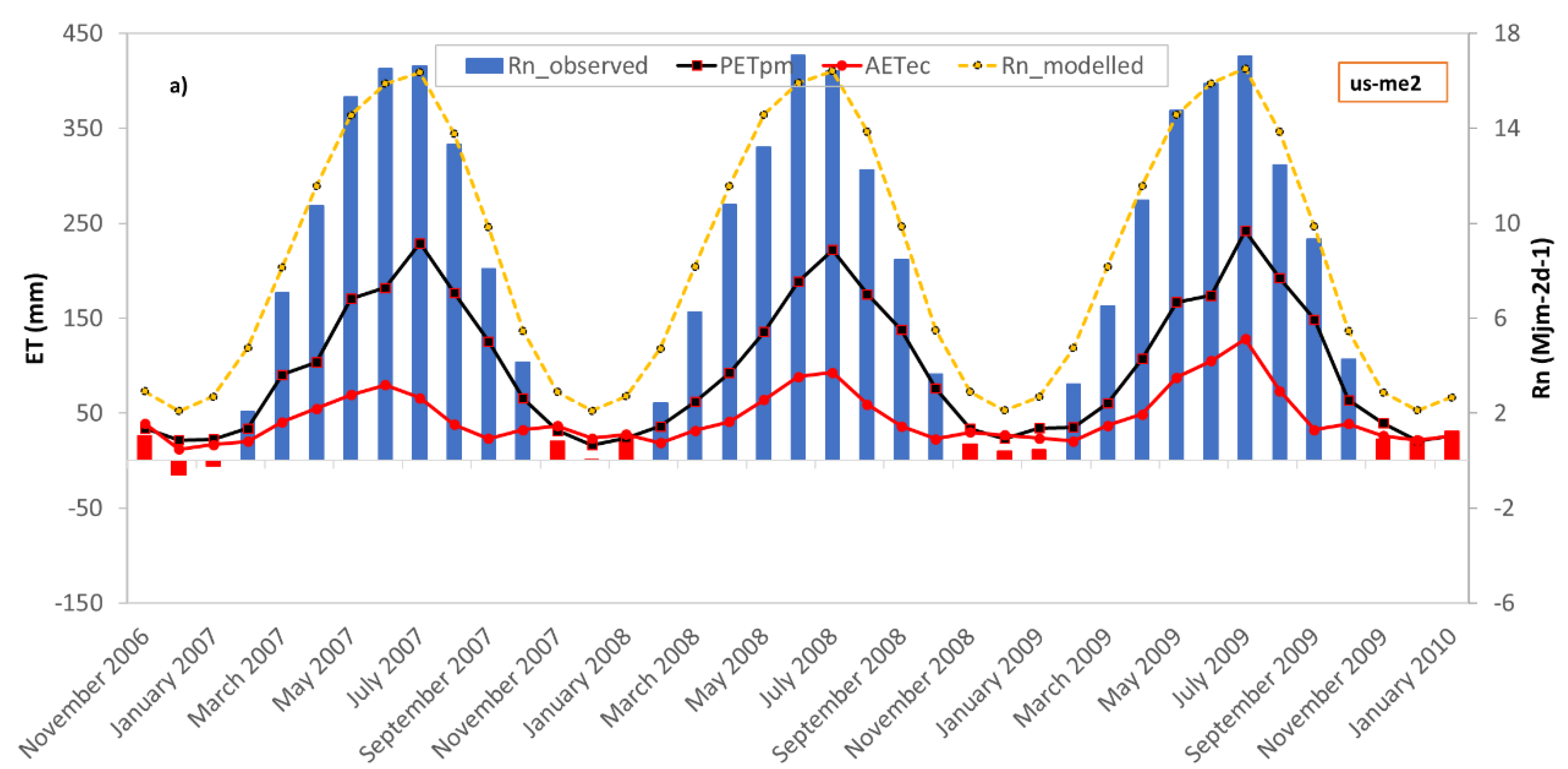
Monthly patterns of precipitation P and potential evapotranspiration PETPM (by Penman model) are illustrated in Figure 2 for the three experimental sites. Monthly precipitation patterns clearly indicate a strong seasonality in the case of us-me2, typical of a Mediterranean climate condition, and a rather uniform precipitation distribution in the cases of de-rur and it-mbo, typical of a temperate oceanic climate condition. Computed on the whole span of available observations, mean annual precipitation and mean annual potential evapotranspiration are approximately 930 mm and 729 mm for the Rollesbroich site, 478 mm and 1247 mm for the Sister site, and 864 mm and 646 for Bondone Mountain. They return, respectively, a Budyko Dryness Index I = P/PETPM [33] of approximately 1.3, 0.4, and 1.3. The energy-limited scheme is thus applicable to the Rollesbroich and Bondone Mountain sites and the water-limited scheme to the Sister site. A comparison between actual evapotranspiration (AETec) derived by eddy covariance observations and PETPM potential evapotranspiration illustrates how, for the three experimental sites, periods where actual rates approach potential ones can be detected. These correspond to the wetter period of the year, between the months of November and February. Actual evapotranspiration rates are lower than PET during the remaining periods, the drier periods, more evidently in the case of the us-me2 site where the gap between actual and potential evapotranspiration processes is significantly different during the water-limited period (Figure 2). The Budyko Dryness Index has been computed at the monthly time scale [33] and illustrated in Figure 2. Even though attention should be paid in interpreting Budyko’s I index on short spatial and temporal scales, as the Budyko’s framework assumes that soil water storage and the macro-climate are at steady state, the seasonality of the I index describes the evapotranspiration intra-annual variability and illustrates a seasonal transition between dry and wet states, that is, between water- and energy-limited conditions [33].
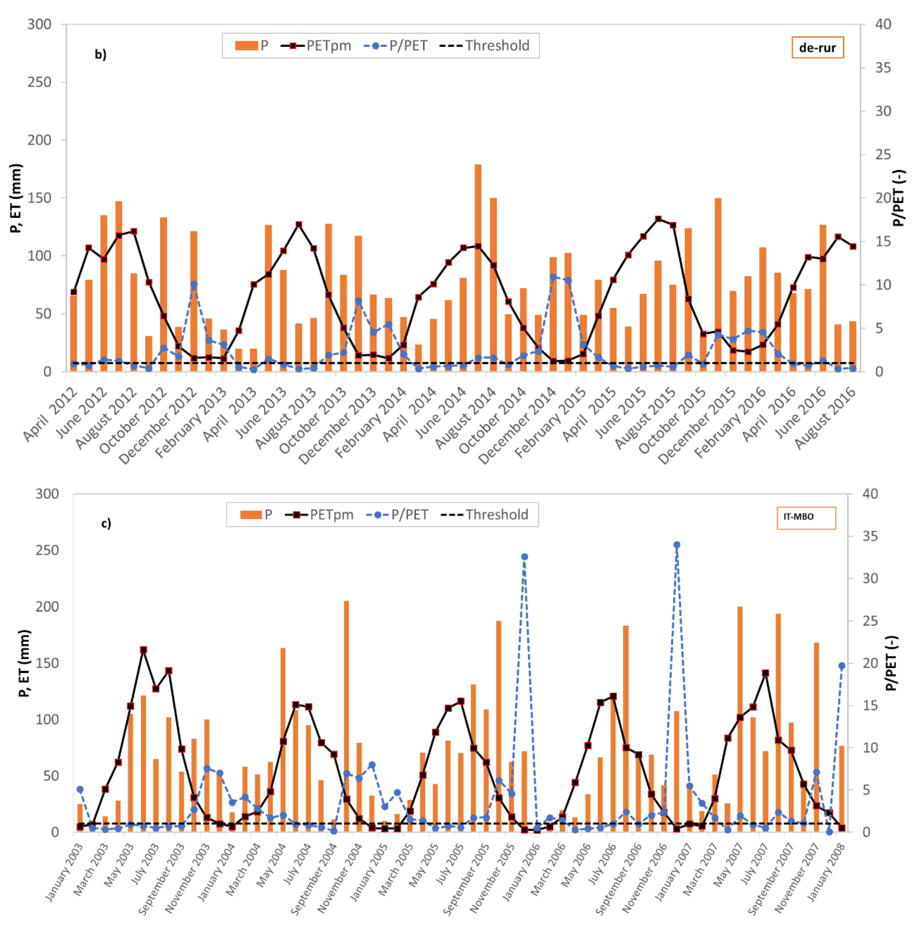
I is generally smaller than the threshold limit of P/PETPM = 1 from March to September for de-rur, from February to October for us-me2 and from March/April to September for it-mbo. During these periods, the systems are assumed as water-limited and, according to the Budyko framework, actual evapotranspiration rates are controlled by precipitation amounts under these conditions. Extraordinary rainfall events (i.e., not consistent with the average behavior) that occurred in July and August of 2014 at the Rollesbroich meteorological station, are the reason why I index is larger than 1 within these months. From November to February in the case of de-rur, from November to January in the case of us-me2, and from November to Febrary/March for it-mbo, index I is instead larger than 1. The transition between dry (water-limited) and wet (energy-limited) dominant states has been found to mainly relate to the seasonal pattern of Rn (Figure 3). In fact, for the three experimental sites, when Rn value is below 2 MJ/m2d−1, actual evapotranspiration, computed at a monthly scale, approaches the potential one. Rn values below this threshold are represented with red bars in Figure 3 and identify the wet energy-limited states.
From Figure 3, it appears that the wet state periods have different lengths for the different sites. For us-me2 the wet state periods last three months, compared to four and five months, respectively, for de-rur and it-mbo. The different duration of the periods where the energy limited scheme is applied can be justified by the soil water storage capacity of the specific sites. Indeed, us-me2 has the highest SWS (99.6 mm) which provides a stronger resistance to water vapor flow from the soil surface to the atmosphere. This is the reason why the Sister site, longer appears water-stressed. Congruently the longer energy limited period for the Bondone Mountain site (it-mbo) is explained by the very small soil water storage capacity.
Provided the illustrated findings related to the temporal transition from dry to wet states, a threshold approach is suggested to more realistically mimic the intra-annual actual evapotranspiration, which couples the Penman (PM) formulation, representing AET during the wet periods (when Rn < 2 MJ/m2d−1), and either the AA (namely PM/AA) or the API (namely PM/API) approaches, representing AET during the dry periods. As previously reported, the transition between states, which is from PM to API (or AA) is provided by the net radiation values. If Rn is the current monthly net radiation and RnT is the mentioned net radiation threshold (2 MJ/m2d−1), the threshold approach results in the following expression:
3.2. Monthly AET Models Evaluation
According to the methods and findings reported, meteorological data-based methods previously discussed have been applied and compared in this study:
- (i)
- the AA, or advection-aridity, method as described by Equation (5);
- (ii)
- the API, or the antecedent precipitation index, method as described by Equation (6);
- (iii)
- the threshold PM/API and PM/AA models as described by Equation (18);
At this stage, a value of the Priestley-Taylor coefficient α equal to 1.26 has been considered in the model evaluation, and the symbolisms API(1.26) and PM/API(1.26) are used to indicate these circumstances. At a first visual inspection, it is possible to observe how, in the cases of the de-rur and it-mbo sites, there is generally a good correspondence between observed and modelled values. An important discrepancy exists instead in the case of the us-me2 site where the API and AA models tend to overestimate (substantially in the case of the API approach) the observed AET values, especially during the dry states (Figure 4), confirming the difficulties in modelling water-limited systems [35]. In the case of the threshold approaches PM/AA and PM/API(1.26), underestimation during the wet periods appears reduced while large overestimation still persists during the dry periods, especially for the methods accounting for the API approach.
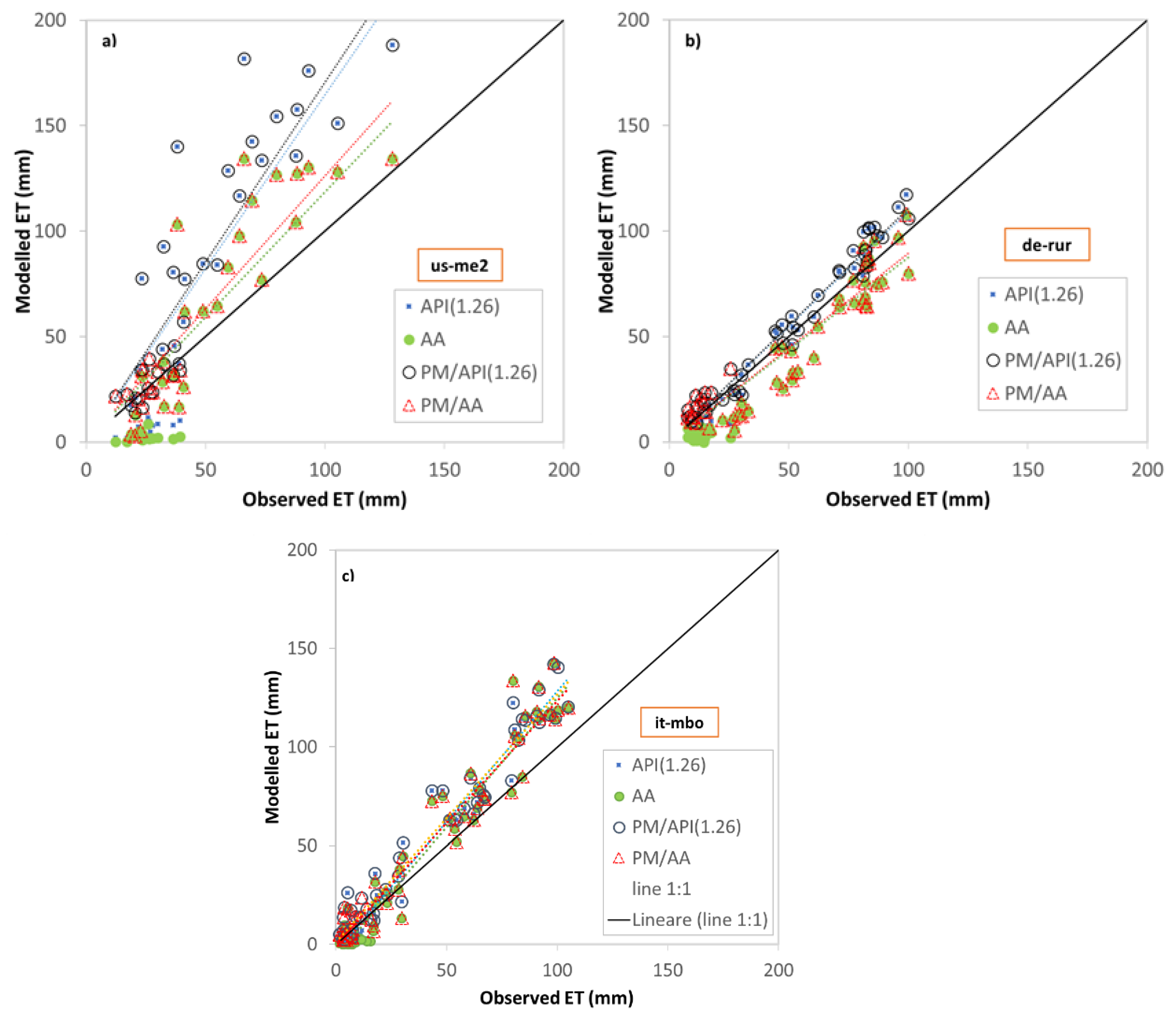
The scatter plots in Figure 5 depict almost the same behavior. A significant scatter exists in the case of the us-me2 site (Figure 5a), which indicates overall a poor agreement between observations and models and large prediction errors. Underestimated observations during the wet state periods (blue and green solid circles on the horizontal axis) disappear when the threshold approach is applied. The same findings, but with a negligible scatter, are found in the cases of the de-rur and it-mbo sites (Figure 5b).
An annual actual evapotranspiration quantitative assessment of the three meteorological data-based methods is reported in Table 2. It is confirmed that, compared to the AETec, which is assumed to be the observed variable, a quantitative large overestimation on the long-term is observed in the case of the Sister site while congruent results are found in the cases of the Rollesbroich site and Bondone Mountain.
To quantify the model performances in predicting AET water losses, the goodness-of-fit indices evaluation is illustrated in Table 3. Over the whole period of observation, the best performing model results the API approach for de-rur and the AA method for us-me2 and it-mbo. Over the full record of observation, the use of the threshold approach to mimic intra-annual ET variability only improves RMSEd by 15% in the case of the us-me2 site, of about 10% in the case of the de-rur site and close to 8% in the case of it-mbo. The pattern agreement index d and the correlation coefficients r also show a moderate improvement for both experimental sites.
Model prediction capabilities do not appear to significantly improve on the long-term scale. In the case of the Sister site, this is probably due to the short length of the wet period (about three months over the year) for which the threshold approach produces a correction. In the case of the Rollesbroich site and Bondone Mountain, the general agreement showed by the basic AA and API model with observed data might be the cause. Differences in terms of performances are more evident when the goodness-of-fit indices are computed separately for the wet and dry periods (Table 4). During the wet period PM/API and PM/AA actually represent the same model (the PM) and for this reason they are featured by the same errors.
Large performance improvements are associated with the threshold model (Equation (18)). In the case of the de-rur site, the normalized RMSEd reduces by about 34%, whereas the agreement index d and the correlation coefficient increased, respectively, by about 70% and 3%. In the case of the us-me2 site, improvements are even more evident with normalized RMSEd, which reduced by about four times, as well as with the increase in the correlation coefficient. A moderate improvement is also detected for the pattern agreement index of about 14%. In the case of the Bondone Mountain site, the RMSEd descreases by about 20% while the index of agreement moved from 0.81 to 0.87. A clear improvement is achieved for r which increases by more than 100%. The performances of the models are still moderate in the case of the dry state period (Table 5). During this period there is of course no benefit from using the threshold approach (PM/AA and PM/API goodness-of-fit indices in Table 5 are the same of the AA and API respectively). AA still appears the best performing in the case of us-me2 and it-mbo whereas better prediction is achieved with the API approach in the case of the de-rur site.
3.3. Models Estimates Using Rn and Gsoil from Empirical Formulas
The empirical formulas used in case of lack of measured data to compute the net radiation and soil heat flux, return average errors in the region of 2.80 mm for Rn and 0.32 mm for Gsoil. Overall, the modelled Rn fluxes tend to overestimate the observed ones as clearly deduced from Figure 6. The mechanism of the switch between dry and wet dominant states remains unchanged, with the only difference being that net radiation threshold is estimated to be around 4 MJ/m2d−1. RnT doubles in value compared to the previous case, probably due to the estimation error committed by the used empirical relationships.
The results of the models evaluation suggest that the AA method is confirmed to be the best-performing approach. Over the full period of observation, the use of a threshold approach improves at most of 7% the ET prediction. During the dry state periods there is no benefit in using the threshold approaches while the benefit is more evident during the wet state periods where the RMSE decreases up to a maximum of 67% (Table 6).
3.4. AET Models Calibration
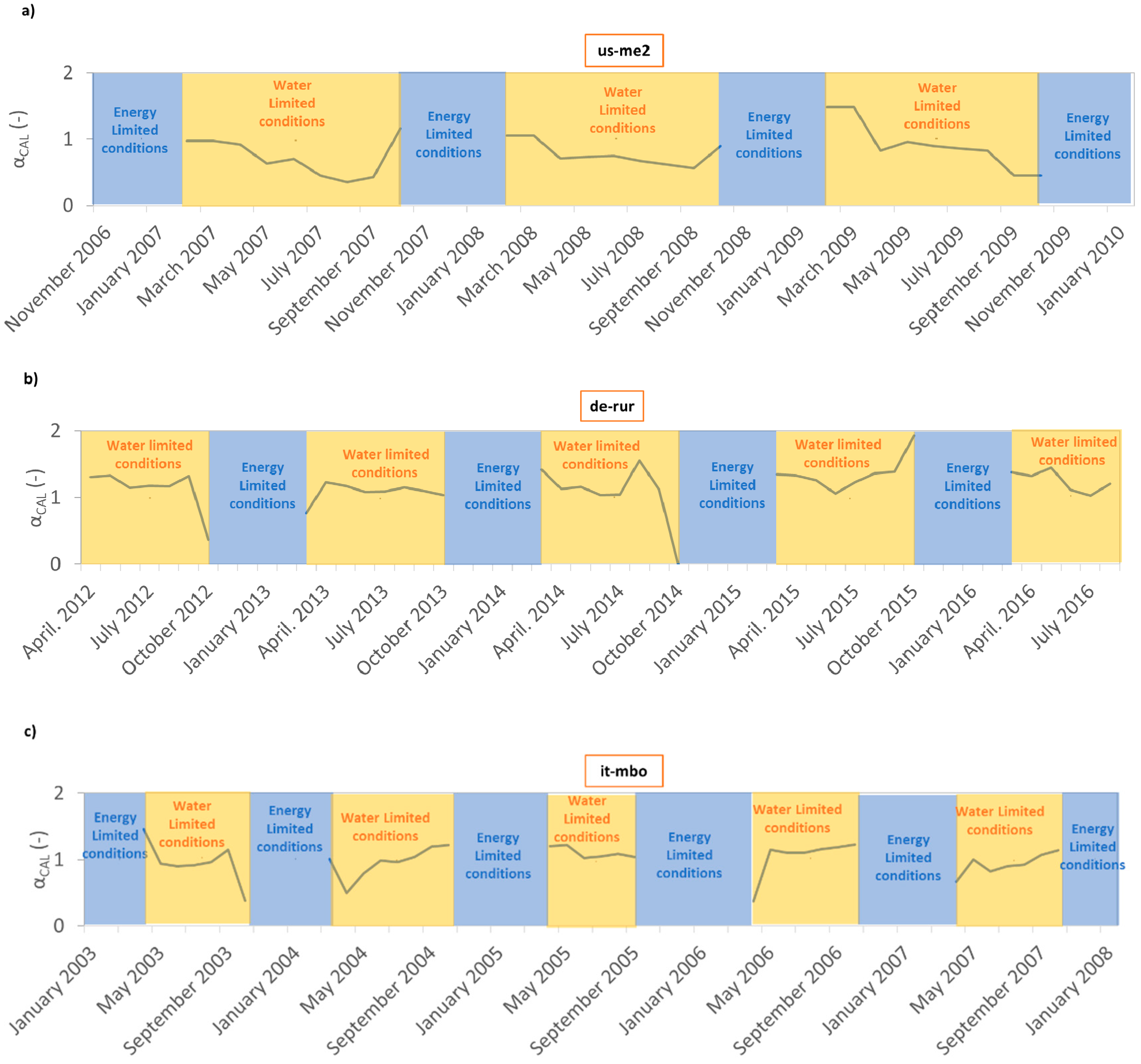
The threshold approach has significantly improved the monthly scale prediction of evaporative demands during the wet state periods, in particular for the Mediterranean forested Sister site water-limited system. Overestimation still persists during the dry periods of limited water availability. To further improve the prediction during this specific time window and, after all, to further improve the description of the intra-annual variability of ET on the long-term scale, a calibration of the Priestley-Taylor coefficient has been necessary. Many authors in the past have argued about the need for the calibration of the α coefficient in the formulation of PT in order to improve ET prediction [64,65]. Although the original value of α proposed by Mawdsley and Ali [22] is 1.26, a moderate range of variability has been reported for such a coefficient in the relevant literature. McNaughton and Black [66] suggested the use of α = 1.05; Davies and Allen [67] proposed a coefficient of 1.27, while Morton [68] proposed a coefficient of approximately 1.32 (similar to the 1.31 value proposed by Hobbins et al. [69]. De Bruin and Keijman [70] further argued that the variation of α lies between 1.15 and 1.42. A wider range of variability, between 1.07 and 2.20, was predicted by Cristea et al. [71]. Fundamentally, no clear tendency in terms of climate and vegetation cover appears from the literature. To follow the intra-annual evapotranspiration dynamic, a monthly scale calibration of the value of the Priestley-Taylor coefficient, α, is proposed in the current study using the eddy covariance data (AETec) as a constraint. The calibration involved the API method. A calibration of α from the AA method is not foreseen as besides the Priestley-Taylor coefficient, the AA model is also potentially affected by the calibration of the wind function [72,73,74]. Furthermore, the calibration only refers to the dry water-limited periods as it is aimed to improve the prediction during this specific span of time. With reference to the API method, assuming that, at the monthly scale (i.e., that the actual evapotranspiration losses computed by the API method as described by Equation (6) during the i-th month equals the ET losses computed from the observed EC fluxes during the same i-th month):
the α coefficient can be computed, at the monthly scale, reversing Equation (19) to derive
where the AETec losses are assumed to correspond to the observed eddy correlation values, and “i” represents the monthly index.
The monthly patterns for the calibrated Priestley-Taylor coefficient during the dry state periods show a relatively stationary value for the αCAL coefficient for the three experimental sites, a condition that makes the assumption of an average constant parameter rather reliable (Figure 7). An average value of αCAL approximatively equal to 1.22 for de-rur, 0.71 for us-me2, and 0.99 for it-mbo has been found. The similarity between the conventional value of α = 1.26 and αCAL = 1.22 for the case of the Rollesbroich site is probably due to the relatively small prediction errors exhibited by the basic model API. In the case of the us-me2 and it-mbo sites, the calibrated α estimate is consistent with a recent investigation [75], which reports about the calibration of the Priestley-Taylor coefficient under a gradient of climate and land cover conditions.
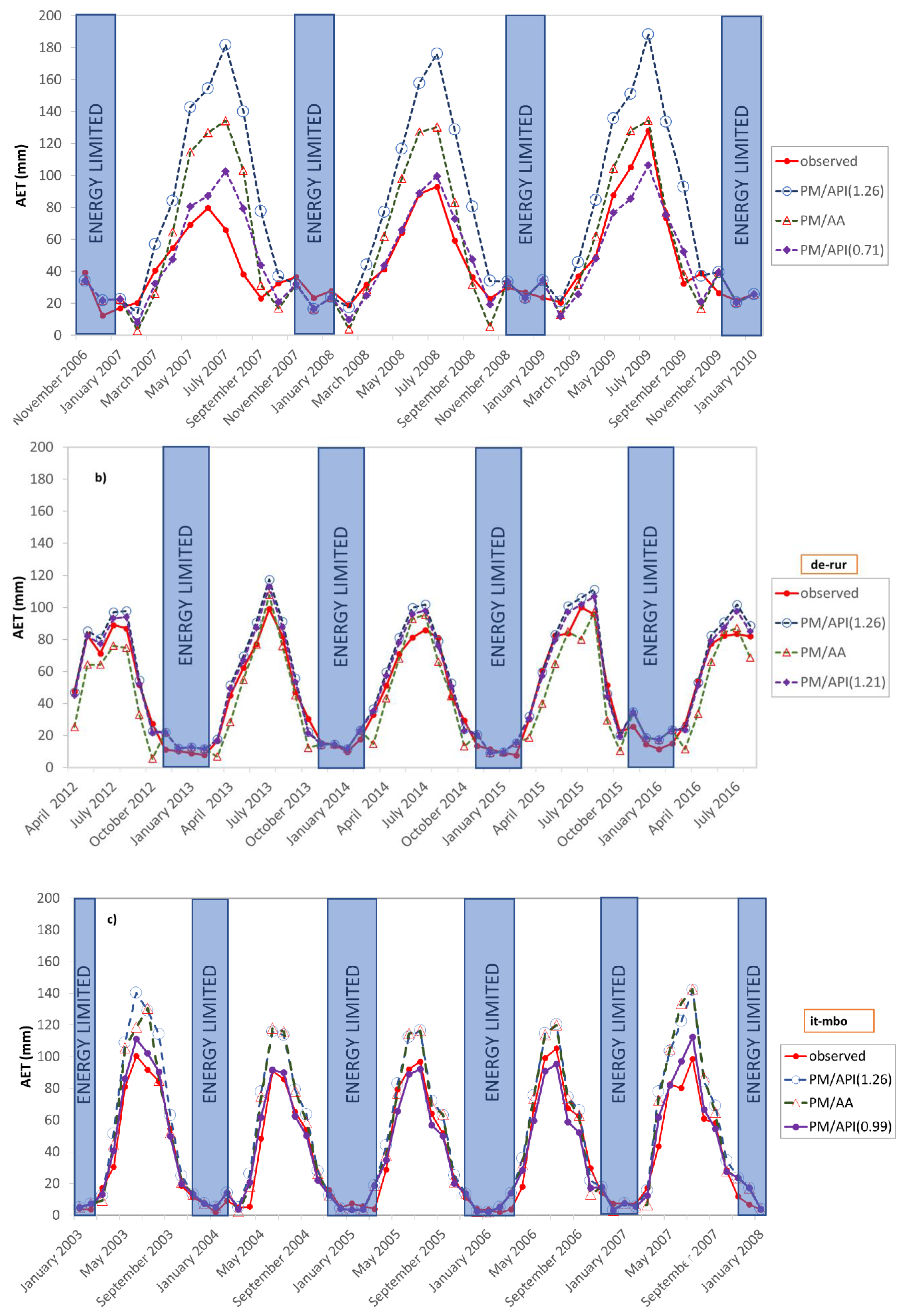
The accuracy of the AET values prediction provided by the calibrated API models, with αCAL = 1.22 for the Rollesbroich site, αCAL = 0.71 for the Sister site, and αCAL = 0.71 for the Bondone Mountain site has been tested and compared to those resulting from the non-calibrated models by using both a visual inspection (Figure 8 and Figure 9) and the quantification of goodness-of-fit indices (Table 3, Table 4 and Table 5).
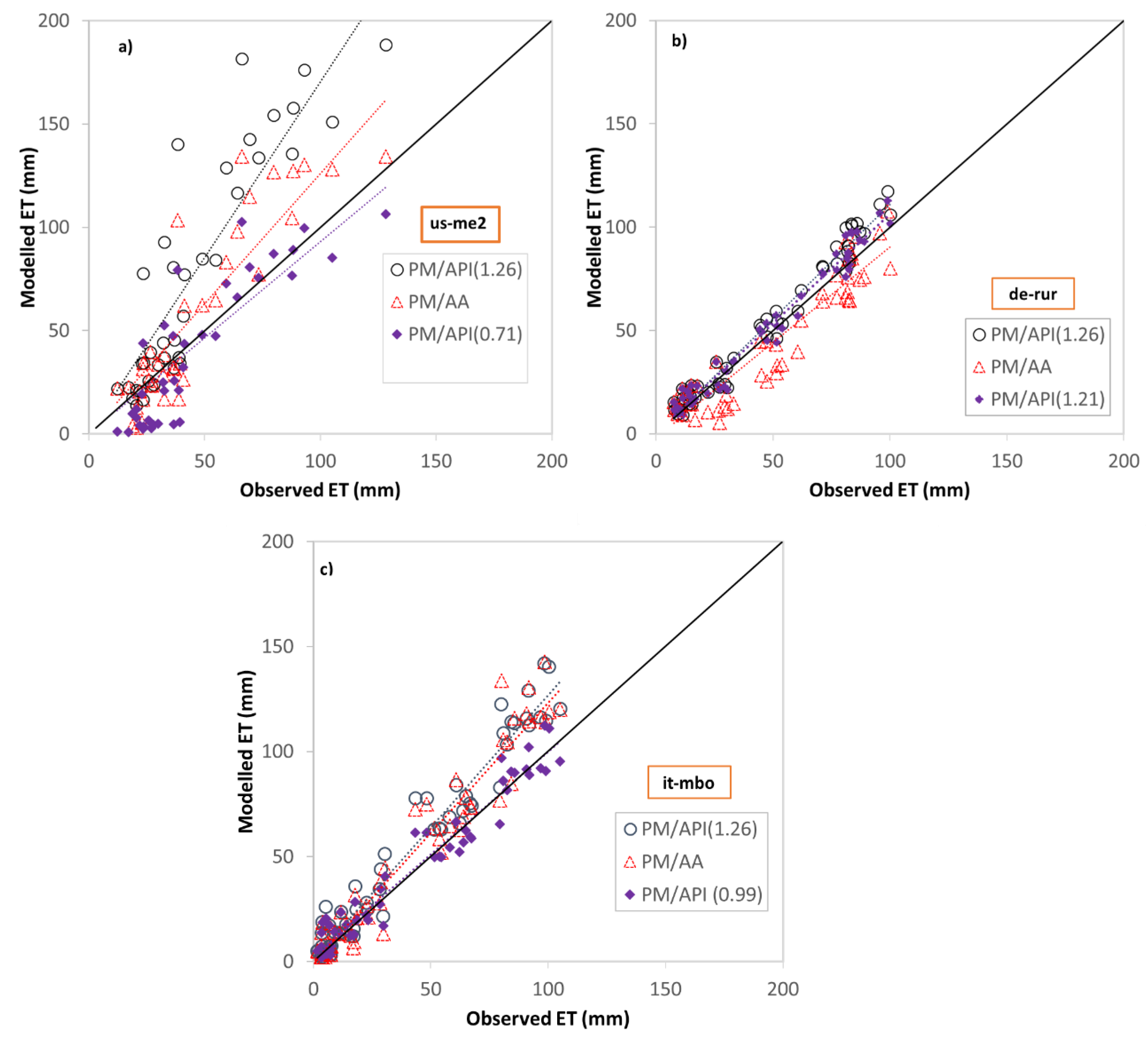
Clearly because of the calibration, as evident from the patterns illustrated in Figure 8 and the quantification provided in Table 2, monthly actual evapotranspiration losses provided by the PM/APICAL approach appear to be more consistent with the EC measurements. From the scatter plots illustrated in Figure 9, it is also evident how the large scatter that characterizes the prediction for the Sister sites by the non-calibrated approaches (Figure 5) is removed from the calibration of α. These circumstances are also supported by the goodness-of-fit assessment. Both for the whole period of observation and the dry state periods, the calibrated threshold approach (PM/APICAL), represents a significant improvement compared to the remaining evaluated approaches (Table 3 and Table 5). Error magnitudes are reduced by about 80% for the Sister site, about 30% in the case of the Rollesbroich site, and 60% for Bondone Mountain.
4. Conclusions
The aim of this study was to propose a meteorological data-based monthly scale model able to predict the intra-annual variability of actual evapotranspiration losses, marking the temporal transition between dry and wet dominant states which would drive the transition from one model to another for AET assessment. The research has been carried out with the support of AET flux observations over multi-year periods for three EC stations located in Rollesbroich (Germany), Sister (Oregon), and Trento (Italy). The literature review suggested that there is not a single approach able to outperform other modeling methods for a particular biome and, without claiming to find very general rules for specific biomes for the ET assessment, the current study explain how, in some circumstances, switching between AET models for a single site in different seasons might help improve evapotranspiration losses assessment. The transition from dry to wet state conditions occurs for a threshold value of net radiation of 2 MJ/m2d−1. The ability of basic AA and API approaches to model intra-annual evapotranspiration has been evaluated and compared to the performances of a proposed threshold approach, which couples PET and basic AET relationships. Large performance improvements are associated with the threshold model in the case of the wet states period assessment. The RMSEd reduction was about 34% in the case of de-rur site, about 20% for Bondone mountain, and for the Sister site, the normalized RMSE reduced about four times. The large overestimation that still persists during the dry state periods has been improved by a calibration of α-coefficient. In this case, for both the whole period of observation and the dry periods, the calibrated threshold approach (PM/APICAL), returns promising results. Error magnitudes are reduced by about 80% for the Sister site, about 30% in the case of the Rollesbroich site, and about 60% for Bondone Mountain. Poor improvement was detected for the whole period of observation by the threshold approach in the absence of the α-coefficient calibration. In the case of the Rollesbroich site and Bondone Moutain site, it might be seen in the general agreement showed by the basic AA and API models with observed data. The implementation of the threshold approach requires the use of net radiation and soil heat fluxes as input parameters. If measured data of Rn and Gsoil are not available at the experimental site, they can be estimated using empirical formulas. The use of empirical formulas to predict these variables affects neither the switch mechanism nor the detection of the wet and dry state periods, it only impacts the value of the net radiation threshold. Indeed, RnT increases from about 2 to 4 MJ/m2d−1,probably due to the overestimation produced by the empirical relationships. However, an improvement in the assessment of Rn from climate data would be important to propose an approach fully based on climate data. An extension of this analysis to more experimental sites, featured by different climate characteristics and land covers, would help foster and strengthen the relevant findings, but is very unlikely to find general rules. Potentially, equitant systems, those systems that straddle the energy–water limited area and for which the switching between the two states is more marked, could more evidently benefit from the proposed findings.
Author Contributions
Conceptualization, A.L.; Methodology, A.L., M.S.; Validation, M.M.; Formal analysis, M.M.; investigation, A.L. and M.M.; Data curation, M.S.; Writing—original draft preparation, A.L and M.M.; Writing—review and editing, A.L., M.M., M.S.; Supervision, A.L. and M.S. All authors have read and agreed to the published version of the manuscript.
Funding
This research received no external funding.
Acknowledgments
This work used eddy covariance data acquired and shared by the FLUXNET com-munity, including these networks: AmeriFlux, AfriFlux, AsiaFlux, CarboAfrica, Car-boEuropeIP, CarboItaly, CarboMont, ChinaFlux, Fluxnet-Canada, GreenGrass, ICOS, KoFlux, LBA, NECC, OzFlux-TERN, TCOS-Siberia, and USCCC. The ERA-Interim reanalysis data are provided by ECMWF and processed by LSCE. The FLUXNET eddy covariance data processing and harmonization was carried out by the European Fluxes Database Cluster, AmeriFlux Management Project, and Fluxda-ta project of FLUXNET, with the support of CDIAC and ICOS Ecosystem Thematic Center, and the OzFlux, ChinaFlux and AsiaFlux offices. The authors also gratefully acknowledge the support of TERENO, funded by the Helmholtz Association, and the SFB-TR32 “Pattern in Soil–Vegetation–Atmosphere Systems: Monitoring, Modeling and Data Assimilation”, funded by the Deutsche Forschungsgemeinschaft (DFG). The Metolius AmeriFlux research was supported by the Office of Science (BER), U.S. Department of Energy, Grant No. DE-FG02-06ER64318. The research was supported by the U.S. Department of Energy’s Office of Science (Grant No. DE-FG02-06ER64318 and DE-AC02-05CH11231 for the AmeriFlux core site) and the US Department of Energy (Grant DE-SC0012194) and Agriculture and Food Research Initiative of the US Department of Agriculture National Institute of Food and Agriculture (Grants 2013-67003-20652, 2014-67003-22065, and 2014-35100-22066) for our North American Carbon Program studies, “Carbon cycle dynamics within Oregon’s urban-suburban-forested-agricultural landscapes”.
Conflicts of Interest
The authors declare no conflict of interest.
References
- McMahon, T.A.; Peel, M.C.; Lowe, L.; Srikanthan, R.; McVicar, T.R. Estimating actual, potential, reference crop and pan evaporation using standard meteorological data: A pragmatic synthesis. Hydrol. Earth Syst. Sci. 2013, 17, 1331–1363. [Google Scholar] [CrossRef] [Green Version]
- Sartor, J.; Mobilia, M.; Longobardi, A. Results and findings from 15 years of sustainable urban storm water management. Int. J. Saf. Secur. Eng. 2018, 8, 505–514. [Google Scholar] [CrossRef]
- Mobilia, M.; Longobardi, A. Model Details, Parametrization, and Accuracy in Daily Scale Green Roof Hydrological Conceptual Simulation. Atmosphere 2020, 11, 575. [Google Scholar] [CrossRef]
- Fortuniak, K.; Pawlak, W.; Bednorz, L.; Grygoruk, M.; Siedlecki, M.; Zieliński, M. Methane and carbon dioxide fluxes of a temperate mire in Central Europe. Agric. For. Meteorol. 2017, 232, 306–318. [Google Scholar] [CrossRef]
- Muhammad, M.K.I.; Nashwan, M.S.; Shahid, S.; Ismail, T.B.; Song, Y.H.; Chung, E.-S. Evaluation of Empirical Reference Evapotranspiration Models Using Compromise Programming: A Case Study of Peninsular Malaysia. Sustainability 2019, 11, 4267. [Google Scholar] [CrossRef] [Green Version]
- Penman, H.L. Natural evaporation from open water, bare soil and grass. Proc. R. Soc. London. Ser. A Math. Phys. Sci. 1948, 193, 120–145. [Google Scholar] [CrossRef] [Green Version]
- Penman, H.L. Vegetation and Hydrology. Soil Sci. 1963, 96, 357. [Google Scholar] [CrossRef]
- Monteith, J.L. Evaporation and environment. In Symposia of the Society for Experimental Biology; Cambridge University Press (CUP): Cambridge, UK, 1965; Volume 19, pp. 205–234. [Google Scholar]
- Priestley, C.H.B.; Taylor, R.J. On the Assessment of Surface Heat Flux and Evaporation Using Large-Scale Parameters. Mon. Weather Rev. 1972, 100, 81–92. [Google Scholar] [CrossRef]
- Hargreaves, G.H.; Samani, Z.A. Estimating of potential evapotranspiration. J. Irrig. Drain. Eng. 1982, 108, 223–230. [Google Scholar]
- Thornthwaite, C.W. An approach toward a rational classification of climate. Geograph. Rev. 1948, 38, 55–94. [Google Scholar] [CrossRef]
- Gangopadhyaya, M.; Uryvaev, V.A.; Omar, M.H.; Nordenson, T.J.; Harbeck, G.E. Measurement and Estimation of Evaporation and Evapotranspiration; W.M.O. Technical Note; World Meteorological Organization: Geneva, Switzerland, 1966. [Google Scholar]
- Dalton, J. Experimental essays on the constitution of mixed gases: On the force of steam or vapour from water or other liquids in different temperatures, both in a Torricelli vacuum and in air; on evaporation; and on expansion of gases by heat. Manch. Lit. Phil. Soc. Mem. Proc. 1802, 5, 536–602. [Google Scholar]
- Ershadi, A.; McCabe, M.F.; Evans, J.; Chaney, N.; Wood, E.F. Multi-site evaluation of terrestrial evaporation models using FLUXNET data. Agric. For. Meteorol. 2014, 187, 46–61. [Google Scholar] [CrossRef]
- Su, Z. The Surface Energy Balance System (SEBS) for estimation of turbulent heat fluxes. Hydrol. Earth Syst. Sci. 2002, 6, 85–100. [Google Scholar] [CrossRef]
- Menenti, M.; Choudhury, B.J. Parameterization of Land Surface Evaporation by Means of Location Dependent Potential Evaporation and Surface Temperature Range; Department for Environment; Food and Rural Affairs (Defra): London, UK, 1993; Volume 212, pp. 561–568. [Google Scholar]
- Bastiaanssen, W.; Pelgrum, H.; Wang, J.; Ma, Y.; Moreno, J.; Roerink, G.; Van Der Wal, T. A remote sensing surface energy balance algorithm for land (SEBAL). J. Hydrol. 1998, 212, 213–229. [Google Scholar] [CrossRef]
- Yates, D.; Strzepek, K.M. Potential Evapotranspiration Methods and Their Impact on the Assessment of River Basin Runoff under Climate Change; WP-94-046; IIASA: Laxenburg, Austria, 1994. [Google Scholar]
- Wang, K.; Dickinson, R.E.; Wild, M.; Liang, S. Evidence for decadal variation in global terrestrial evapotranspiration between 1982 and 2002: 1. Model development. J. Geophys. Res. Space Phys. 2010, 115, 20. [Google Scholar] [CrossRef] [Green Version]
- Fisher, J.; Tu, K.P.; Baldocchi, D. Global estimates of the land–atmosphere water flux based on monthly AVHRR and ISLSCP-II data, validated at 16 FLUXNET sites. Remote Sens. Environ. 2008, 112, 901–919. [Google Scholar] [CrossRef]
- Ding, R.; Kang, S.; Li, F.; Zhang, Y.; Tong, L. Evapotranspiration measurement and estimation using modified Priestley–Taylor model in an irrigated maize field with mulching. Agric. For. Meteorol. 2013, 168, 140–148. [Google Scholar] [CrossRef]
- Mawdsley, J.A.; Ali, M.F. Estimating Nonpotential Evapotranspiration by Means of the Equilibrium Evaporation Concept. Water Resour. Res. 1985, 21, 383–391. [Google Scholar] [CrossRef]
- Bouchet, R.J. Evapotranspiration réelle et potentielle, signification climatique. IAHS Publ. 1963, 62, 134–142. [Google Scholar]
- Jian, D.; Li, X.; Sun, H.; Tao, H.; Jiang, T.; Su, B.; Hartmann, H. Estimation of Actual Evapotranspiration by the Complementary Theory-Based Advection–Aridity Model in the Tarim River Basin, China. J. Hydrometeorol. 2018, 19, 289–303. [Google Scholar] [CrossRef]
- Chu, R.; Li, M.; Islam, A.R.M.T.; Fei, D.; Shen, S. Attribution analysis of actual and potential evapotranspiration changes based on the complementary relationship theory in the Huai River basin of eastern China. Int. J. Clim. 2019, 39, 4072–4090. [Google Scholar] [CrossRef]
- Zhang, T.; Gebremichael, M.; Meng, X.; Wen, J.; Iqbal, M.; Jia, D.; Li, Z. Climate-related trends of actual evapotranspiration over the Tibetan Plateau (1961–2010). Int. J. Climatol. 2018, 38, e48–e56. [Google Scholar] [CrossRef]
- Granger, R.; Gray, D. Evaporation from natural nonsaturated surfaces. J. Hydrol. 1989, 111, 21–29. [Google Scholar] [CrossRef]
- Armstrong, R.N.; Pomeroy, J.W.; Martz, L.W. Estimating Evaporation in a Prairie Landscape under Drought Conditions. Can. Water Resour. J. 2010, 35, 173–186. [Google Scholar] [CrossRef] [Green Version]
- Morton, F. Estimating evapotranspiration from potential evaporation: Practicality of an iconoclastic approach. J. Hydrol. 1978, 38, 1–32. [Google Scholar] [CrossRef]
- Xu, Z.; Li, J.Y. Estimating Basin Evapotranspiration Using Distributed Hydrologic Model. J. Hydrol. Eng. 2003, 8, 74–80. [Google Scholar] [CrossRef]
- Otsuki, K.; Mitsuno, T.; Maruyama, T. Comparison between water budget and complementary relationship estimates of catchment evapotranspiration. Trans. Jpn. Soc. Irrig. Drain. Reclam Eng. 1984, 112, 17–23. [Google Scholar]
- Szilagyi, J.; Hobbins, M.; Józsa, J. Modified Advection-Aridity Model of Evapotranspiration. J. Hydrol. Eng. 2009, 14, 569–574. [Google Scholar] [CrossRef] [Green Version]
- Ryu, Y.; Baldocchi, D.; Ma, S.; Hehn, T. Interannual variability of evapotranspiration and energy exchange over an annual grassland in California. J. Geophys. Res. Space Phys. 2008, 113, 2156–2202. [Google Scholar] [CrossRef] [Green Version]
- Longobardi, A.; Khaertdinova, E. Relating soil moisture and air temperature to evapotranspiration fluxes during inter-storm periods at a Mediterranean experimental site. J. Arid. Land 2014, 7, 27–36. [Google Scholar] [CrossRef]
- Zhang, D.; Liu, X.; Zhang, Q.; Liang, K.; Liu, C. Investigation of factors affecting intra-annual variability of evapotranspiration and streamflow under different climate conditions. J. Hydrol. 2016, 543, 759–769. [Google Scholar] [CrossRef]
- Zheng, H.; Yu, G.-R.; Wang, Q.; Zhu, X.; Yan, J.; Wang, H.; Shi, P.; Zhao, F.; Li, Y.; Zhao, L.; et al. Assessing the ability of potential evapotranspiration models in capturing dynamics of evaporative demand across various biomes and climatic regimes with ChinaFLUX measurements. J. Hydrol. 2017, 551, 70–80. [Google Scholar] [CrossRef]
- McVicar, T.R.; Roderick, M.L.; Donohue, R.J.; Van Niel, T.G. Less bluster ahead? Ecohydrological implications of global trends of terrestrial near-surface wind speeds. Ecohydrology 2012, 5, 381–388. [Google Scholar] [CrossRef]
- Wang, D. Evaluating interannual water storage changes at watersheds in Illinois based on long-term soil moisture and groundwater level data. Water Resour. Res. 2012, 48, 03502. [Google Scholar] [CrossRef]
- Liu, G.; Liu, Y.; Hafeez, M.; Xu, D.; Vote, C. Comparison of two methods to derive time series of actual evapotranspiration using eddy covariance measurements in the southeastern Australia. J. Hydrol. 2012, 454, 1–6. [Google Scholar] [CrossRef]
- Temesgen, B.; Eching, S.O.; Davidoff, B.; Frame, K. Comparison of Some Reference Evapotranspiration Equations for California. J. Irrig. Drain. Eng. 2005, 131, 73–84. [Google Scholar] [CrossRef]
- Ministry of Agriculture. Soil Water Storage Capacity and Available Soil Moisture; Water conservation factsheet; Ministry of Agriculture: Victoria, BC, Canada, 2015. [Google Scholar]
- Kwon, H.; Law, B.; Thomas, C.K.; Johnson, B. The influence of hydrological variability on inherent water use efficiency in forests of contrasting composition, age, and precipitation regimes in the Pacific Northwest. Agric. For. Meteorol. 2018, 249, 488–500. [Google Scholar] [CrossRef]
- Brown, R.N.; Percivalle, C.; Narkiewicz, S.; DeCuollo, S. Relative Rooting Depths of Native Grasses and Amenity Grasses with Potential for Use on Roadsides in New England. HortScience 2010, 45, 393–400. [Google Scholar] [CrossRef]
- Post, H.; Franssen, H.-J.H.; Graf, A.; Schmidt, M.; Vereecken, H. Uncertainty analysis of eddy covariance CO2 flux measurements for different EC tower distances using an extended two-tower approach. Biogeosciences 2015, 12, 1205–1221. [Google Scholar] [CrossRef] [Green Version]
- Gebler, S.; Franssen, H.-J.H.; Pütz, T.; Post, H.; Schmidt, M.; Vereecken, H. Actual evapotranspiration and precipitation measured by lysimeters: A comparison with eddy covariance and tipping bucket. Hydrol. Earth Syst. Sci. 2015, 19, 2145–2161. [Google Scholar] [CrossRef] [Green Version]
- Marcolla, B.; Cescatti, A.; Manca, G.; Zorer, R.; Cavagna, M.; Fiora, A.; Gianelle, D.; Rodeghiero, M.; Sottocornola, M.; Zampedri, R. Climatic controls and ecosystem responses drive the inter-annual variability of the net ecosystem exchange of an alpine meadow. Agric. For. Meteorol. 2011, 151, 1233–1243. [Google Scholar] [CrossRef]
- Suttie, J.M.; Reynolds, S.G.; Batello, C. Grasslands of the World; Food and Agriculture Organization of the United Nations: Rome, Italy, 2005. [Google Scholar]
- Carlowicz, M. Seeing Forests for the Trees and the Carbon: Mapping the World’s Forests in Three Dimensions; Earth Observatory: Washington, DC, USA, 2012. [Google Scholar]
- Allen, R.G.; Pereira, L.S.; Raes, D.; Smith, M. Crop Evapotranspiration-Guidelines for Computing Crop Water Requirements-FAO Irrigation and Drainage Paper 56; FAO: Rome, Italy, 1998. [Google Scholar]
- Reichstein, M.; Falge, E.; Baldocchi, D.; Papale, D.; Aubinet, M.; Berbigier, P.; Bernhofer, C.; Buchmann, N.; Gilmanov, T.; Granier, A.; et al. On the separation of net ecosystem exchange into assimilation and ecosystem respiration: Review and improved algorithm. Glob. Chang. Biol. 2005, 11, 1424–1439. [Google Scholar] [CrossRef]
- Chebbi, R.Z.; Prévot, L.; Chakhar, A.; Abdallah, M.M.-B.; Jacob, F. Observing Actual Evapotranspiration from Flux Tower Eddy Covariance Measurements within a Hilly Watershed: Case Study of the Kamech Site, Cap Bon Peninsula, Tunisia. Atmosphere 2018, 9, 68. [Google Scholar] [CrossRef] [Green Version]
- Papale, D.; Reichstein, M.; Aubinet, M.; Canfora, E.; Bernhofer, C.; Kutsch, W.; Longdoz, B.; Rambal, S.; Valentini, R.; Vesala, T.; et al. Towards a standardized processing of Net Ecosystem Exchange measured with eddy covariance technique: Algorithms and uncertainty estimation. Biogeosciences 2006, 3, 571–583. [Google Scholar] [CrossRef] [Green Version]
- Bogawski, P.; Bednorz, E. Comparison and Validation of Selected Evapotranspiration Models for Conditions in Poland (Central Europe). Water Resour. Manag. 2014, 28, 5021–5038. [Google Scholar] [CrossRef] [Green Version]
- Guo, D.; Westra, S.; Maier, H.R. Sensitivity of potential evapotranspiration to changes in climate variables for different Australian climatic zones. Hydrol. Earth Syst. Sci. 2017, 21, 2107–2126. [Google Scholar] [CrossRef] [Green Version]
- Moratiel, R.; Snyder, R.L.; Durán, J.M.; Tarquis, A.M. Trends in climatic variables and future reference evapotranspiration in Duero Valley (Spain). Nat. Hazards Earth Syst. Sci. 2011, 11, 1795–1805. [Google Scholar] [CrossRef] [Green Version]
- Wang, W.-G.; Zou, S.; Luo, Z.-H.; Zhang, W.; Chen, D.; Kong, J. Prediction of the Reference Evapotranspiration Using a Chaotic Approach. Sci. World J. 2014, 2014, 347625. [Google Scholar] [CrossRef]
- Xu, C.-Y.; Singh, V.P. Evaluation of three complementary relationship evapotranspiration models by water balance approach to estimate actual regional evapotranspiration in different climatic regions. J. Hydrol. 2005, 308, 105–121. [Google Scholar] [CrossRef]
- Shifa, Y.B. Estimation of Evapotranspiration Using Advection Aridity Approach. Master Thesis, University of Twente Faculty of Geo-Information and Earth Observation (ITC), Enschede, The Netherlands, 2011. [Google Scholar]
- Narayanan, P. Evaluation of Performance of Evapotranspiration Models in Selected Climatic Regions in the United States. Ph.D. Thesis, University of Massachusetts, Amherst, USA, 1989. [Google Scholar]
- Brutsaert, W.; Stricker, H. An advection-aridity approach to estimate actual regional evapotranspiration. Water Resour. Res. 1979, 15, 443–450. [Google Scholar] [CrossRef]
- Koehler, M.A.; Linsley, R.K. Predicting the Runoff from Storm Rainfall, Research Paper n.34; Weather Bureau, US Dept of Commerce: Washington, DC, USA, 1951. [Google Scholar]
- Marasco, D.E.; Culligan, P.J.; McGillis, W.R. Evaluation of common evapotranspiration models based on measurements from two extensive green roofs in New York City. Ecol. Eng. 2015, 84, 451–462. [Google Scholar] [CrossRef] [Green Version]
- Mobilia, M.; Longobardi, A.; Sartor, J.F. Including A-Priori Assessment of Actual Evapotranspiration for Green Roof Daily Scale Hydrological Modelling. Water 2017, 9, 72. [Google Scholar] [CrossRef] [Green Version]
- Irmak, S.; Irmak, A.; Allen, R.G.; Jones, J.W. Solar and Net Radiation-Based Equations to Estimate Reference Evapotranspiration in Humid Climates. J. Irrig. Drain. Eng. 2003, 129, 336–347. [Google Scholar] [CrossRef]
- Tabari, H.; Grismer, M.E.; Trajkovic, S. Comparative analysis of 31 reference evapotranspiration methods under humid conditions. Irrig. Sci. 2011, 31, 107–117. [Google Scholar] [CrossRef]
- McNaughton, K.G.; Black, T.A. A study of evapotranspiration from a Douglas fir forest using the energy balance approach. Water Resour. Res. 1973, 9, 1579–1590. [Google Scholar] [CrossRef] [Green Version]
- Davies, J.A.; Allen, C.D. Equilibrium, Potential and Actual Evaporation from Cropped Surfaces in Southern Ontario. J. Appl. Meteorol. 1973, 12, 649–657. [Google Scholar] [CrossRef] [Green Version]
- Morton, F. Operational estimates of areal evapotranspiration and their significance to the science and practice of hydrology. J. Hydrol. 1983, 66, 1–76. [Google Scholar] [CrossRef]
- Hobbins, M.; Ramirez, J.A.; Brown, T.C. The complementary relationship in estimation of regional evapotranspiration: An enhanced advection-aridity model. Water Resour. Res. 2001, 37, 1389–1403. [Google Scholar] [CrossRef] [Green Version]
- De Bruin, H.A.R.; Keijman, J.Q. The Priestley-Taylor Evaporation Model Applied to a Large, Shallow Lake in the Netherlands. J. Appl. Meteorol. 1979, 18, 898–903. [Google Scholar] [CrossRef] [Green Version]
- Cristea, N.; Kampf, S.K.; Burges, S.J. Revised Coefficients for Priestley-Taylor and Makkink-Hansen Equations for Estimating Daily Reference Evapotranspiration. J. Hydrol. Eng. 2013, 18, 1289–1300. [Google Scholar] [CrossRef] [Green Version]
- Pruitt, W.O.; Doorenbos, J. Empirical calibration, a requisite for evaporation formulae based on daily or longer mean climatic data? In Proceedings of the ICID Conference on Evapotranspiration, Budapest, Hungary, 26–28 May 1977.
- Jensen, D.T.; Hargreaves, G.H.; Temesgen, B.; Allen, R.G. Computation of ETo under Nonideal Conditions. J. Irrig. Drain. Eng. 1997, 123, 394–400. [Google Scholar] [CrossRef]
- Martínez-Cob, A.; Tejero-Juste, M. A wind-based qualitative calibration of the Hargreaves ET0 estimation equation in semiarid regions. Agric. Water Manag. 2004, 64, 251–264. [Google Scholar] [CrossRef] [Green Version]
- Mobilia, M.; Longobardi, A. Evaluation of meteorological data-based models for potential and actual evapotranspiration losses using flux measurements. In Prooceedings of the 20th International Conference on Computational Science and Its Applications 2020, Cagliari, Italy, 1–4 July 2020; Gervasi, O., Murgante, B., Misra, S., Garau, C., Blecic, I., Taniar, D., Apduhan, B., Rocha, A., Tarantino, E., Torre, C., et al., Eds.; Springer: Cham, Switzerland, 2020. [Google Scholar]
Figure 1.
Experimental sites location. Sister site (a), Rollesbroich site (b), Bondone Mountain site (c).
Figure 1.
Experimental sites location. Sister site (a), Rollesbroich site (b), Bondone Mountain site (c).

Figure 2.
Monthly rainfall, Penman potential evapotranspiration and Budyko Index I = P/PET at Sister site (a), Rollesbroich site (b) and Bondone Mountain (c) for the period under investigation. The threshold of Rn has been set at 2 MJ/m2d−1.
Figure 2.
Monthly rainfall, Penman potential evapotranspiration and Budyko Index I = P/PET at Sister site (a), Rollesbroich site (b) and Bondone Mountain (c) for the period under investigation. The threshold of Rn has been set at 2 MJ/m2d−1.


Figure 3.
Monthly actual evapotranspiration, Penman potential evapotranspiration, and net radiation at the Sister site (a), the Rollesbroich site (b), and Bondone mountain (c) for the period under investigation. Red bars indicate net radiation values below the net radiation threshold.
Figure 3.
Monthly actual evapotranspiration, Penman potential evapotranspiration, and net radiation at the Sister site (a), the Rollesbroich site (b), and Bondone mountain (c) for the period under investigation. Red bars indicate net radiation values below the net radiation threshold.

Figure 4.
Monthly patterns for AET computed by the empirical and threshold approaches at the Sister site (a), the Rollesbroich site (b), and Bondone mountain (c). The energy limited period has been highlighted where the threshold approaches have a larger fitting. (AA = advection-aridity method; API (1.26) = API corrected potential evapotranspiration, with α = 1.26; PM/AA = Penman/advection-aridity threshold model; PM/API(1.26) = Penman/API corrected potential evapotranspiration threshold model, with α = 1.26).

Figure 5.
Scatter plots of observed and modelled ET values at the Sister site (a), the Rollesbroich site (b), and Bondone mountain (c). (AA = advection-aridity method; API (1.26) = API corrected potential evapotranspiration, with α = 1.26; PM/AA = Penman/advection-aridity threshold model; PM/API(1.26) = Penman/API corrected potential evapotranspiration threshold model, with α = 1.26).

Figure 6.
Monthly actual evapotranspiration, Penman potential evapotranspiration and observed and modelled net radiation at Sister site (a), Rollesbroich site (b) and Bondone mountain (c) for the period under investigation. Red bars indicate net radiation values below the net radiation threshold.
Figure 6.
Monthly actual evapotranspiration, Penman potential evapotranspiration and observed and modelled net radiation at Sister site (a), Rollesbroich site (b) and Bondone mountain (c) for the period under investigation. Red bars indicate net radiation values below the net radiation threshold.


Figure 7.
Monthly patterns for the calibrated αCAL coefficient at us-me2 (a), de-rur (b) and it-mbo during water limited periods.
Figure 7.
Monthly patterns for the calibrated αCAL coefficient at us-me2 (a), de-rur (b) and it-mbo during water limited periods.

Figure 8.
Monthly patterns for AET computed by the empirical and threshold approaches at Sister site (a), Rollesbroich site (b), and and Bondone mountain (c). The energy limited period has been highlighted where the threshold approaches have a larger fitting. (PM/AA = Penman/advection-aridity threshold model; PM/API(1.26) = Penman/API corrected potential evapotranspiration threshold model, with α = 1.26; PM/API(αCAL) = Penman/API corrected potential evapotranspiration calibrated threshold model).

Figure 9.
Scatter plots of observed and modelled ET values at Sister site (a), Rollesbroich site (b) and and Bondone mountain (c). (PM/AA = Penman/advection-aridity threshold model; PM/API(1.26) = Penman/API corrected potential evapotranspiration threshold model, with α = 1.26; PM/API(αCAL) = Penman/API corrected potential evapotranspiration calibrated threshold model).


Table 1.
Missing values for the three sites.
| Name | Record Period | Number of Days (-) | Number of 30 min Intervals (-) | Missing LE (%) |
|---|---|---|---|---|
| de-rur | 2012 to 2016 | 1614 | 77472.0 | 5.9 |
| us-me2 | 2006 to 2010 | 1188 | 57024.0 | 5.1 |
| it-mbo | 2003 to 2008 | 1829 | 87744.0 | 0.01 |
Table 2.
Annual actual evapotranspiration losses from the EC flux data (AETec) and from the compared meteorological data-based approach models (AA = advection-aridity method; API (1.26) = API corrected potential evapotranspiration, with α = 1.26; PM/AA = Penman/advection-aridity threshold model; PM/API(1.26) = Penman/API corrected potential evapotranspiration threshold model, with α = 1.26; PM/APICAL = Penman/API corrected potential evapotranspiration calibrated threshold model).
| a) us-me2 | ||||||
|---|---|---|---|---|---|---|
| AETec (mm) | AA (mm) | API(1.26) (mm) | PM/AA (mm) | PM/API(1.26) (mm) | PM/APICAL (mm) | |
| Total | 562.19 | 606.75 | 891.52 | 681.25 | 952.69 | 574.87 |
| b) de-rur | ||||||
| Total | 536.15 | 416.34 | 551.44 | 472.76 | 595.33 | 574.39 |
| c) it-mbo | ||||||
| Total | 471.22 | 543.04 | 574.75 | 578.04 | 605.70 | 488.49 |
Table 3.
Goodness-of-fit indices for the four applied models. Errors are computed on monthly AET time series for the whole period of observation (AA = the advection-aridity method; API (1.26) = the API corrected potential evapotranspiration with α = 1.26; PM/AA = the Penman/advection-aridity threshold model; PM/API(1.26) = the Penman/API corrected potential evapotranspiration threshold model with α = 1.26; PM/APICAL = Penman/API corrected potential evapotranspiration calibrated threshold model).
| Whole Period of Observation | |||||
|---|---|---|---|---|---|
| RMSE (mm) | RMSEd (-) | d(-) | r(-) | EQ. | |
| a) us-me2 | |||||
| AA | 27.04 | 0.60 | 0.66 | 0.90 | (5) |
| API (1.26) | 49.02 | 1.08 | 0.51 | 0.85 | (6) |
| PM/AA | 23.69 | 0.52 | 0.71 | 0.90 | (18) |
| PM/API(1.26) | 44.98 | 0.99 | 0.54 | 0.89 | |
| PM/APICAL(0.71) | 13.40 | 0.30 | 0.78 | 0.89 | (18) + αCAL |
| b) de-rur | |||||
| RMSE (mm) | RMSEd (-) | d(-) | r(-) | EQ. | |
| AA | 12.91 | 0.27 | 0.81 | 0.97 | (5) |
| API (1.26) | 8.89 | 0.19 | 0.88 | 0.99 | (6) |
| PM/AA | 11.83 | 0.25 | 0.83 | 0.94 | (18) |
| PM/API(1.26) | 8.32 | 0.17 | 0.89 | 0.99 | |
| PM/APICAL(1.22) | 6.64 | 0.14 | 0.90 | 0.99 | (18) + αCAL |
| c) it-mbo | |||||
| RMSE (mm) | RMSEd (-) | d(-) | r(-) | EQ. | |
| AA | 16.04 | 0.41 | 0.84 | 0.97 | (5) |
| API (1.26) | 16.87 | 0.44 | 0.83 | 0.98 | (6) |
| PM/AA | 15.12 | 0.38 | 0.84 | 0.97 | (18) |
| PM/API(1.26) | 16.80 | 0.43 | 0.83 | 0.98 | |
| PM/APICAL(0.99) | 7.53 | 0.19 | 0.91 | 0.98 | (18) + αCAL |
Table 4.
Goodness-of-fit indices for the four applied models. Errors are computed on monthly AET time series for the wet state period (AA = the advection-aridity method; API (1.26) = the API corrected potential evapotranspiration with α = 1.26; PM/AA = the Penman/advection-aridity threshold model; PM/API(1.26) = the Penman/API corrected potential evapotranspiration threshold model with α = 1.26; PM/APICAL = Penman/API corrected potential evapotranspiration calibrated threshold model).
| Wet State Period | |||||
|---|---|---|---|---|---|
| RMSE (mm) | RMSEd (-) | d(-) | r(-) | EQ. | |
| a) us-me2 | |||||
| AA | 24.45 | 0.94 | 0.84 | 0.16 | (5) |
| API (1.26) | 19.71 | 0.76 | 0.87 | 0.71 | (6) |
| PM/AA = PM/API(1.26) = PM/APICAL(0.71) | 6.78 | 0.26 | 0.96 | 0.55 | (18); (18) + αCAL |
| b) de-rur | |||||
| AA | 12.82 | 0.73 | 0.38 | 0.79 | (5) |
| API (1.26) | 6.98 | 0.40 | 0.66 | 0.88 | (6) |
| PM/AA = PM/API(1.26) = PM/APICAL(1.22) | 5.21 | 0.30 | 0.67 | 0.82 | (18); (18) + αCAL |
| c) it-mbo | |||||
| AA | 6.87 | 1.02 | 0.81 | 0.06 | (5) |
| API (1.26) | 6.09 | 0.91 | 0.82 | 0.26 | (6) |
| PM/AA = PM/API(1.26) = PM/APICAL(0.99) | 5.58 | 0.83 | 0.87 | 0.56 | (18); (18) + αCAL |
Table 5.
Goodness-of-fit indices for the four applied models. Errors are computed on monthly AET time series for the dry state period (AA = the advection-aridity method; API (1.26) = the API corrected potential evapotranspiration with α = 1.26; PM/AA = the Penman/advection-aridity threshold model; PM/API(1.26) = the Penman/API corrected potential evapotranspiration threshold model with α = 1.26; PM/APICAL = Penman/API corrected potential evapotranspiration calibrated threshold model).
| Dry State Period | |||||
|---|---|---|---|---|---|
| RMSE (mm) | RMSEd (-) | d(-) | r(-) | EQ. | |
| a) us-me2 | |||||
| AA | 28.11 | 0.52 | 0.81 | 0.88 | (5) |
| API (1.26) | 53.87 | 1.00 | 0.66 | 0.87 | (6) |
| PM/AA | 28.11 | 0.52 | 0.81 | 0.88 | (18) |
| PM/API(1.26) | 53.87 | 1.00 | 0.66 | 0.87 | |
| PM/APICAL(0.71) | 15.46 | 0.29 | 0.88 | 0.86 | (18) + αCAL |
| b) de-rur | |||||
| AA | 12.99 | 0.18 | 0.68 | 0.91 | (5) |
| API (1.26) | 10.20 | 0.14 | 0.76 | 0.96 | (6) |
| PM/AA | 12.99 | 0.18 | 0.68 | 0.91 | (14) |
| PM/API(1.26) | 10.20 | 0.14 | 0.76 | 0.96 | |
| PM/APICAL(1.22) | 7.55 | 0.10 | 0.81 | 0.96 | (18) + αCAL |
| c) it-mbo | |||||
| AA | 19.60 | 0.34 | 0.89 | 0.95 | (5) |
| API (1.26) | 20.84 | 0.36 | 0.87 | 0.96 | (6) |
| PM/AA | 19.60 | 0.34 | 0.89 | 0.95 | (14) |
| PM/API(1.26) | 20.84 | 0.36 | 0.87 | 0.96 | |
| PM/APICAL(1.22) | 8.49 | 0.15 | 0.94 | 0.96 | (18) + αCAL |
Table 6.
RMSE (mm) the four applied models using Rn and G derived from empirical relationships. Errors are computed on monthly AET time series for the dry state period (AA = the advection-aridity method; API (1.26) = the API corrected potential evapotranspiration with α = 1.26; PM/AA = the Penman/advection-aridity threshold model; PM/API(1.26) = the Penman/API corrected potential evapotranspiration threshold model with α = 1.26; PM/APICAL = Penman/API corrected potential evapotranspiration calibrated threshold model).
| Whole Period of Observation | Wet State Period | Dry State Period | |
|---|---|---|---|
| a) us-me2 | |||
| AA | 27.72 | 19.68 | 30.63 |
| API (1.26) | 49.21 | 9.92 | 58.78 |
| PM/AA | 25.76 | 6.78 | 30.63 |
| PM/API(1.26) | 49.05 | 6.78 | 58.78 |
| b) de-rur | |||
| AA | 21.23 | 9.14 | 27.47 |
| API (1.26) | 26.70 | 8.10 | 35.33 |
| PM/AA | 20.78 | 5.21 | 27.47 |
| PM/API(1.26) | 26.71 | 5.21 | 35.33 |
| c) it-mbo | |||
| AA | 38.36 | 12.36 | 47.64 |
| API (1.26) | 37.31 | 16.91 | 45.40 |
| PM/AA | 36.41 | 5.58 | 47.64 |
| PM/API(1.26) | 36.56 | 5.58 | 45.40 |
© 2020 by the authors. Licensee MDPI, Basel, Switzerland. This article is an open access article distributed under the terms and conditions of the Creative Commons Attribution (CC BY) license (http://creativecommons.org/licenses/by/4.0/).
Share and Cite
MDPI and ACS Style
Mobilia, M.; Schmidt, M.; Longobardi, A. Modelling Actual Evapotranspiration Seasonal Variability by Meteorological Data-Based Models. Hydrology 2020, 7, 50. https://0-doi-org.brum.beds.ac.uk/10.3390/hydrology7030050
AMA Style
Mobilia M, Schmidt M, Longobardi A. Modelling Actual Evapotranspiration Seasonal Variability by Meteorological Data-Based Models. Hydrology. 2020; 7(3):50. https://0-doi-org.brum.beds.ac.uk/10.3390/hydrology7030050
Chicago/Turabian StyleMobilia, Mirka, Marius Schmidt, and Antonia Longobardi. 2020. "Modelling Actual Evapotranspiration Seasonal Variability by Meteorological Data-Based Models" Hydrology 7, no. 3: 50. https://0-doi-org.brum.beds.ac.uk/10.3390/hydrology7030050
Note that from the first issue of 2016, this journal uses article numbers instead of page numbers. See further details here.