Impact of Climate Change on the Streamflow Modulated by Changes in Precipitation and Temperature in the North Latitude Watershed of Nepal

Abstract

It is unambiguous that climate change alters the intensity and frequency of precipitation and temperature distribution at the global and local levels. The rate of change in temperature in the northern latitudes is higher than the worldwide average. The annual distribution of precipitation over the Himalayas in the northern latitudes shows substantial spatial and temporal heterogeneity. Precipitation and temperature are the major driving factors that impact the streamflow and water availability in the basin, illustrating the importance of research on the impact of climate change on streamflow by varying the precipitation and temperature in the Thuli Bheri River Basin (TBRB). Multiple climate models were used to project and evaluate the precipitation and temperature distribution changes in temporal and spatial domains. To analyze the potential impact of climate change on the streamflow in the basin, the Soil and Water Assessment Tool (SWAT) hydrological model was used. The climate projection was carried out in three future time windows. The result shows that the precipitation fluctuates between approximately +12% and +50%, the maximum temperature varies between −7% and +7%, and the minimum temperature rises from +0.7% to +5% in intermediate- and high-emission scenarios. In contrast, the streamflow in the basin varies from −40% to +85%. Thus, there is a significant trend in the temperature increase and precipitation reduction in the basin. Further, the relationship between precipitation and temperature with streamflow shows a substantial dependency between them. The variability in precipitation and streamflow is successfully represented by the water yield in the basin, which plays an important role in the sustainability of the water-related projects in the basin and downstream to it. This also helps quantify the amount of water available for hydropower generation, agricultural production, and the water ecosystem in the TBRB.

1. Introduction

Climate change (CC) is projected to impact the future precipitation, temperature, and water availability at global [1], regional [2,3], and basin [4,5] scales. As a result, CC will eventually impact the global and regional hydrological cycle, resulting in intense floods and droughts [6]. The situation is exacerbated by other driving forces, such as demography, urbanization, land use and land cover change, and many more [7]. In addition, mushrooming urbanization and increased anthropogenic activities, such as high carbon emission through industrial activities, have inflamed the fluctuations in the hydrological cycle, affecting the entire water distribution in the watershed. Various studies have shown the impact of climate change on the long-term projection of hydro-climatic variables at global, regional, and watershed scales [8,9,10,11,12,13,14,15]. However, only a few studies have been carried out on the impact of climate change in the northern latitudes of Nepal [5,16].

Several studies have been conducted to assess the impact of climate change in the Nepalese river basins using hydrological and climate models [4,17,18]. These studies emphasize the projection and alteration in the precipitation and temperature distribution in the respective river basins and the potential impact on hydropower generation and water availability. However, only a few studies have evaluated the effect of climate change on water yield distribution in future times under intermediate- and high-representative-concentration-pathway (RCP) emission scenarios in the river basins located at the northern latitudes of Nepal [19]. The RCPs describe the extent of the future climate based on the volume of greenhouse gas emissions. For example, RCP 4.5 (intermediate-emission scenario) and RCP 8.5 (high-emission scenario) refer to the radiative forcing of, respectively, 4.5 and 8.5 W/m² by the end of the 21st century [1]. However, they failed to establish the relationship between the climatic variables (precipitation and temperature) and streamflow as precipitation, temperature, and streamflow are sensitive to climate change. Further, few studies have used an ensemble of multiple climate models as an input to drive the hydrological model in simulating the future streamflow [5]. In addition, special attention should be paid to selecting the calibration parameters for efficient snow simulation for snow-fed river basins. Unlike earlier research, this paper aims to evaluate and quantify the likely changes in the precipitation, temperature, streamflow, and water yield under changing climate conditions using multiple climate models in the snow-fed river basins in western Nepal.

Hydrological models are used as one of the major tools in planning water resources for sustainable management. The spatial extent of a hydrological model (HM) varies and can be classified as a lumped or a distributed HM, which can simulate at the global-to-basin scales for various purposes [20,21,22,23,24]. The lumped HM considers the entire watershed as a single unit and does not include the spatial difference in the catchment. However, in the distributed HM, parameters need to be defined for each spatial extent. The Soil and Water Assessment Tool (SWAT) is a semi-distributed HM [25,26] widely used in simulating the streamflow under current and future emission scenarios for both large and small watersheds [16,27,28,29,30,31,32,33,34]. The model uses the hydrological response unit (HRU) as the smallest unit to simulate streamflow and water availability. The regional climate model (RCM) climate data are input into the modeling system to simulate the streamflow for the future time window. As a RCM possesses significant climate biases, it must be corrected before feeding into the SWAT modeling system [4,5,14,17]. Various bias-correcting techniques have been devised [35] to reduce biases. Two popular methods, i.e., linear scaling and quantile mapping (QM), have been widely used to correct biases [17,36].

The Thuli Bheri River Basin (TBRB), one of the subbasins of the Bheri River Basin (BRB), is located in western Nepal in Karnali Province. The basin comprises a snow-fed river, one of the major sources of water transfer to the southern river basins, such as the Babai River Basin (BaRB) in the Lumbini province of the country [19]. The government has started constructing a Bheri Babai Diversion Multipurpose Project (BBDMP) to transfer water from the Bheri River to the BaRB. The latter basin is a water deficit basin aiming to provide year-round irrigation facilities and generate hydroelectricity [37]. Therefore, the intensity and frequency of the precipitation and temperature received in the basin will impact the river’s spatiotemporal variability of water availability.

Moreover, further increase or decrease in the daily/monthly/annual temperature will significantly impact snow melting, fluctuating the streamflow volume in space and time. Thus, the water volume available in the TBRB will ultimately alter the transferring water volume to BaRB. Additionally, the extent of climate change on the water resources in TBRB will eventually impact the water resources’ availability in the BaRB and ultimately affect the planned year-round irrigation, hydropower, and the country’s economy. In this context, a study focusing on the impact of climate change on the future precipitation, temperature, and streamflow, and interdependencies between them would be valuable for the water resource managers and different stakeholders active in BBDMP.

This study aims to assess the projection and changes in precipitation, temperature, streamflow, and water yield and establish the interdependencies of precipitation and temperature against streamflow in the snow-fed TBRB located in the northern latitudes of Nepal using multiple climate models under the intermediate-and high-emission scenario. The research results will help water management authorities of TBRB regulate river water transfer through BBDMP under changing climate in the future. Further, the insights of this study can be employed in other transboundary river basins with similar climatic, geographic, and topographic features.

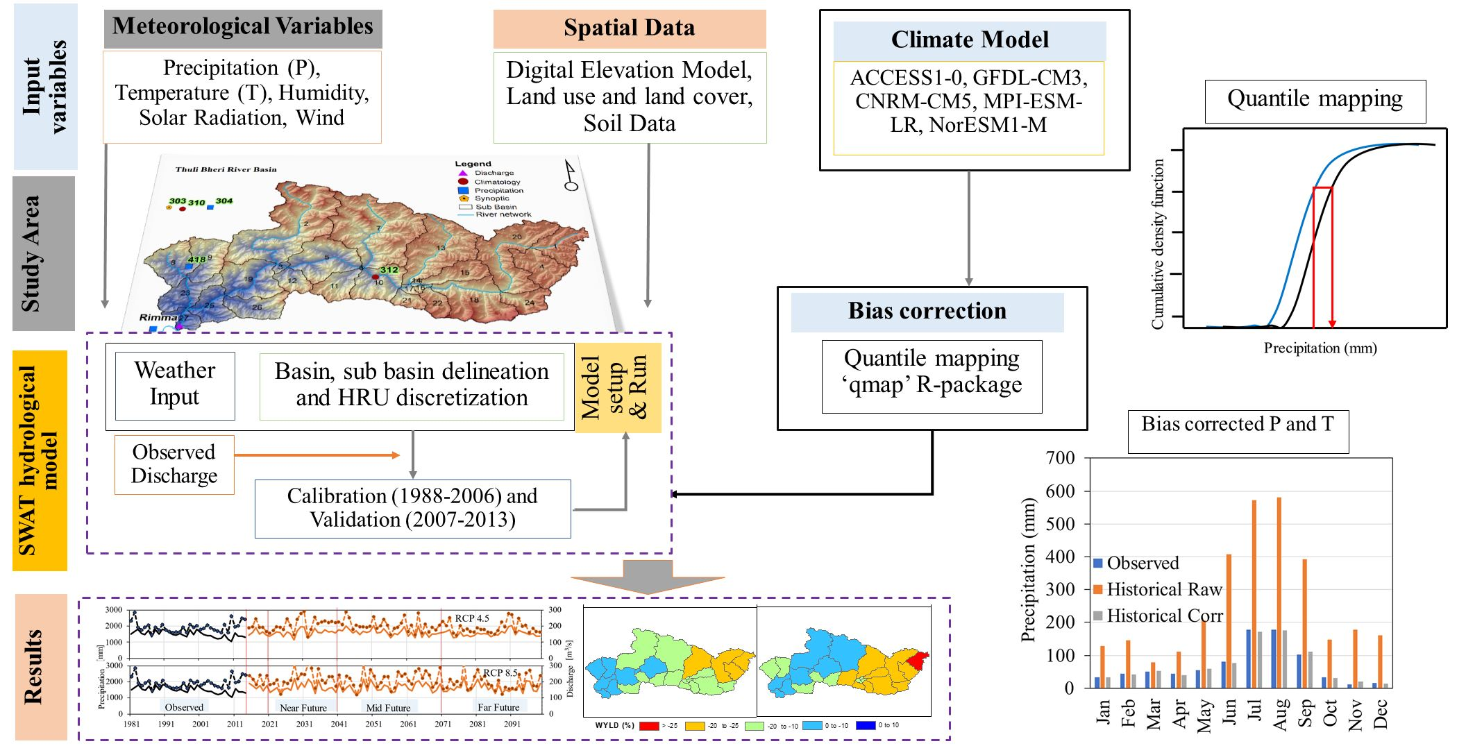
2. Materials and Methods

2.1. Materials

The data required for this research were acquired from various sources, as shown in

Table 1. Characteristics and spatial extent of different data used in the current study.

SN	Data Type	Source	Characteristics		Reference
			Period	Spatial/Temporal Resolution
1	Precipitation	DHM, Nepal	1981–2014	Daily	http://www.dhm.gov.np/ (accessed on 15 July 2018).
2	Temperature
3	Solar Radiation
4	Humidity
5	Wind
6	Streamflow
7	Land use and Land cover	ICIMOD, Nepal	2010	30 m × 30 m	[39]
8	Soil	SOTER-FAO	2009	1:1 Million	[40]
9	Climate Models	CORDEX South Asia RCM Experiment	1981–2100	0.5° × 0.5°	[4,38] http://cccr.tropmet.res.in (accessed on 10 December 2017).
	ACCESS1-0, GFDL-CM3, CNRM-CM5, MPI-ESM-LR, NorESM1-M				Commonwealth Scientific and Industrial Research Organisation (CSIRO)
10	Digital Elevation Model	SRTM	2010	30 m × 30 m

ICIMOD: International Center for Integrated Mountain Development, SOTER-FAO: Soil and Terrain Database-Food and Agricultural Organization, DHM: Department of Hydrology and Meteorology, SRTM-DEM: The shuttle radar topography mission-digital elevation model, CORDEX: coordinated regional climate downscaling experiment.

. The table illustrates the spatial and temporal extent of the acquired datasets and their respective reference material. The hydro-meteorological data were collected from the Department of Hydrology and Meteorology (DHM), Kathmandu, Nepal, and their details are tabulated in Table S1. The spatial data such as land use and land cover (LULC), soil, and digital elevation model (DEM) were collected from the International Centre for Integrated Mountain Development (ICIMOD), soil and terrain database- food and agricultural organization (SOTER-FAO), and the shuttle radar topography mission (SRTM), respectively. The DEM is available at 30 m × 30 m horizontal resolution, one of the high-resolution DEMs used for hydrological modeling purposes. Similarly, the LULC data available from the ICIMOD are also at 30 m × 30 m horizontal resolution. The soil data prepared by SOTER-FAO are available at 1:1 million spatial resolution. The daily climate data with non-homogeneous spatial distribution well represent the study area. The climate models were collected from the coordinated regional climate downscaling experiment (CORDEX) South Asia experiment for climate projections. The climate models were chosen based on their performance in different research carried out in the Himalayan River Basins and considering their spatial and temporal resolution. The CORDEX South Asia RCM is dynamically downscaled from six global climate models (GCMs), namely ACCESS1-0, GFDL-CM3, CNRM-CM5, MPI-ESM-LR, and NorESM-1 M [38]. These climate models have a horizontal resolution of 0.5° × 0.5° and are available for 1971–2005 (historical period) and 2006–2100 (future period). In this study, we used the climate model data from 1981 to 2005 for the historical time window because of the data limitation in the observed data from DHM, and the future climate data were used from 2021 to 2100.

2.2. Methods

2.2.1. Bias Correction of Precipitation and Temperature

The climate model data were extracted to a point scale at gauge stations. Future precipitation and temperature projection were evaluated after correcting bias from the extracted climate model data using the quantile mapping (QM) approach. The QM approach assumes that the bias in the historical data is fixed and will remain the same when projecting the future climates [41]. QM corrects the climate model data’s quantile by matching the observed data’s quantiles by creating a transfer function [35,36]. Empirical QM was used and implemented in the R-programming language using the ‘qmap’ package. The general equation representing the empirical QM technique is shown by Equations (1)–(4):

P_his (d)* = F⁻¹_obs,m {F_his,m (P_his,m)}

(1)

P_sim (d)* = F⁻¹_obs,m {F_sim,m (P_sim,m)}

(2)

T_his (d)* = F⁻¹_obs,m {F_his,m (T_his,m)}

(3)

T_sim (d)* = F⁻¹_obs,m {F_sim,m (T_sim,m)}

(4)

where F is the cumulative distribution function and F⁻¹ is the inverse. P represents precipitation, T represents temperature, and his, sim, and obs represents historical, simulated, and observed, respectively.

The bias-corrected (BC) precipitation and temperature data were projected at monthly and annual scales for future time windows. The future time windows are referred to as Near Future (2021–2040), Mid Future (2041–2070), and Far Future (2071–2100). The Near Future was shortening to 20 years to account for the future climatic variability and provide the equal temporal length of Mid Future and Far Future.

2.2.2. Development of SWAT Hydrological Model

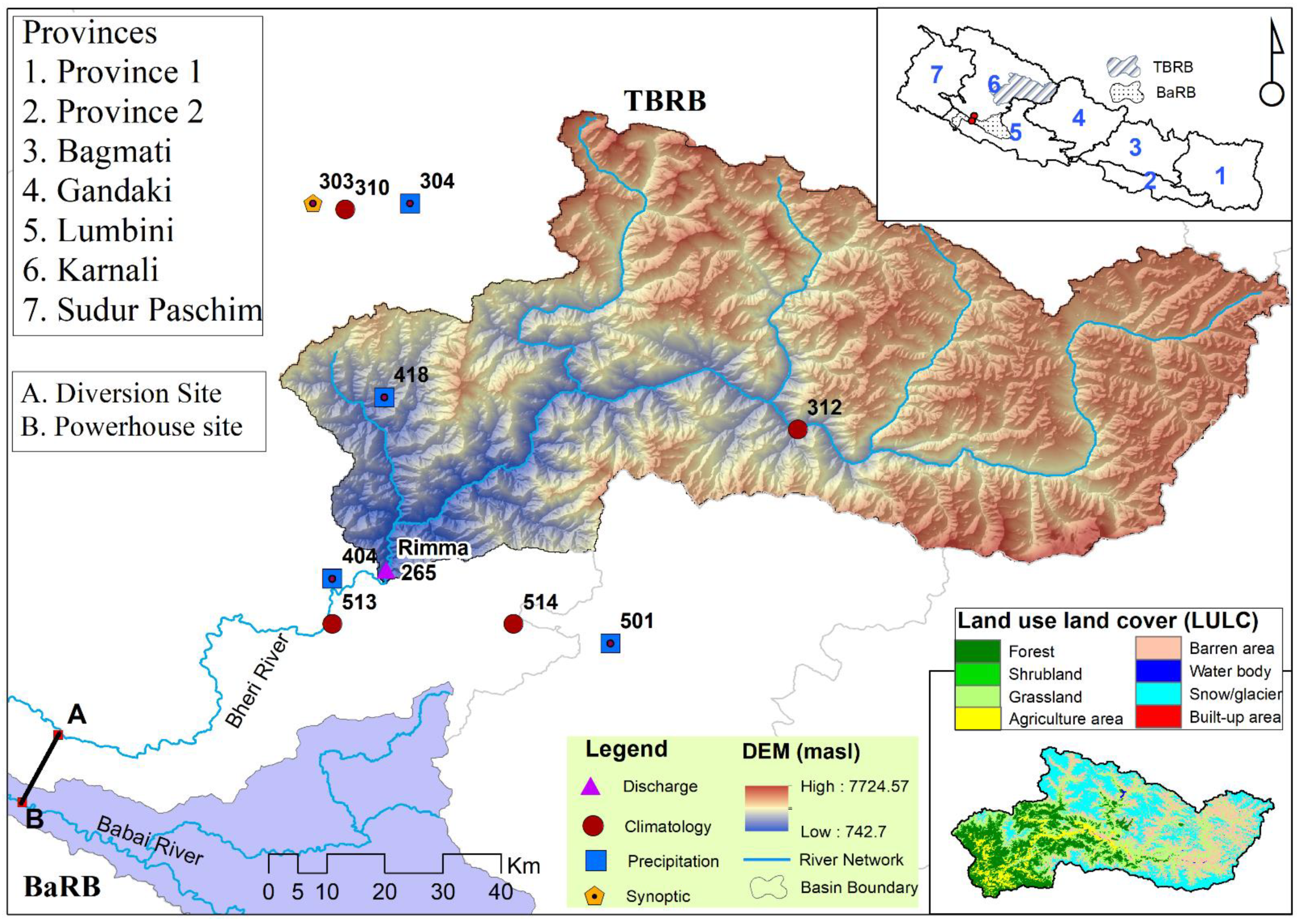
The physically based semi-distributed SWAT hydrological model was developed to simulate the river runoff for historical and future time windows in the TBRB. Firstly, the whole TBRB was divided into 27 sub-basins incorporating the major river tributaries as far as possible. Then, the sub-basins were further divided into 362 hydrologic response units (HRUs) with similar land use, soil, and slopes, taking 2%, 5%, and 10% as thresholds, respectively. The model was then calibrated and validated at the Rimma gauge station (represented by triangle symbol in Figure 1) using the SUFI-2 algorithm in the Soil and Water Assessment Tool-Calibration Uncertainties Program (SWAT-CUP) module considering Nash–Sutcliffe efficiency (NSE) as an objective function. Three iterations, 500 simulations of each, were carried out in SWAT-CUP to improve the parameters’ values in each iteration to meet the objective function. The calibrated parameters were then used in the SWAT model to enhance the efficiency of the model further. Calibration was carried out for 19 years (1988–2006) and then validated for seven years (2007–2013). The bias-corrected projected climate model precipitation and temperature data were then fed into the SWAT model to simulate the future streamflow and water yield in each sub-basin.

2.3. Study Area

The TBRB is one of the sub-basins of the Bheri River Basin system of the Karnali Province in western Nepal. The basin is situated in the upper Himalayas of Nepal, which is snow-fed and extends from 82°16′ E to 83°40′ E to 28° 41′ N to 29°10′ N. It encompasses 6866 km², covering approximately 49.3% of the Bheri River watershed area [19]. As per SRTM-DEM, the vertical elevation in the basin varies from 742.7 m to 7724.0 m above mean sea level (masl). The basin occupies more than 25% of the snow-covered mountains. The grassland (25.4%) and snow cover (25.1%) occupy more than 50% of the total land area of the basin, which is followed by barren land (23.7%). The forest area in the basin covers almost 18.6% of the total basin area. The other land cover types are agriculture (5.3%), shrubland (1.7%), water bodies (0.2%), and built-up (<0.1%). The basin is located in a remote area of the country and is less impacted by human intervention (built-up area <0.1%) [37,40]. The Bheri River, a major tributary of the Karnali River, runs along TBRB and BRB, where the government of Nepal is constructing a multipurpose diversion project. The river drains through the Surkhet district before joining the Karnali River. The national pride project, BBDMP, aims to transfer water from the Bheri River (site A in Figure 1) to Babai River (site B in Figure 1) through a diversion tunnel (shown by the solid black line in Figure 1). The transferred water is proposed to irrigate 51,000 Ha of command area in Banke, Bardiya, and current irrigated land by the Babai Irrigation Project throughout the year and generate 46.8 MW of hydroenergy [37].

3. Results

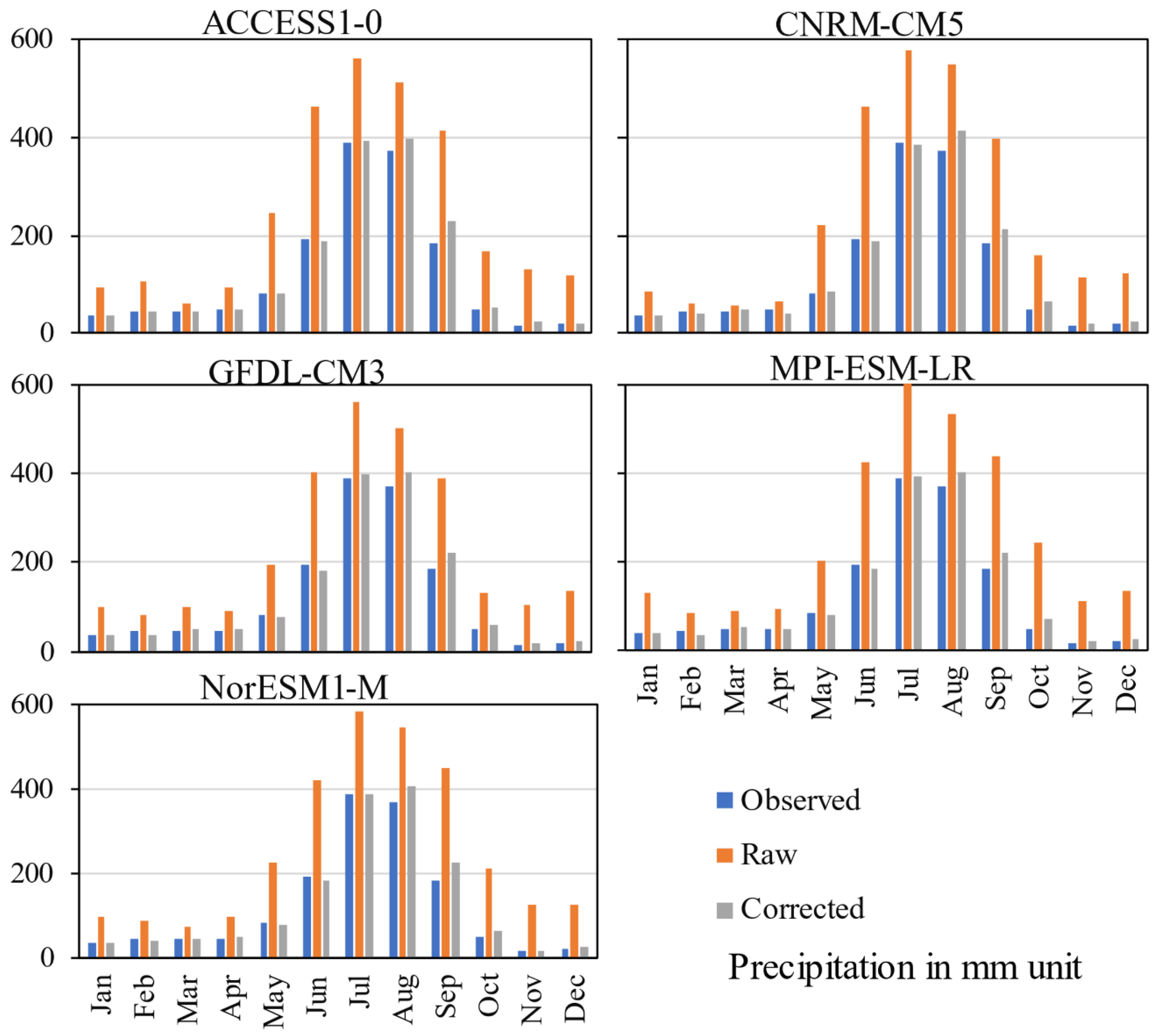
3.1. Statistical Performance of Bias-Corrected Precipitation and Temperature

The ensemble average monthly distribution of precipitation for different climate models before and after bias correction against the observed data is shown in Figure 2. All the climate models overestimated the historical uncorrected precipitation data at all gauge stations. The maximum overestimation in the monthly precipitation was seen at station 303, while the minimum overestimation was at station 418. For example, at station 303 in July, the monthly precipitation was 177.9 mm, while the ACCESS1-0 model was overestimated to be 572.1 mm, which was found to be 172.0 mm after bias correction. Similarly, at station 418 in the same month, the observed precipitation was 531.0 mm, but the ACCESS1-0 model overestimated it to be 618.6 mm. After applying the bias correction, monthly precipitation was found to be 554.8 mm. Similar tendencies were observed at other stations when using the other climate models with varying intensities.

After bias correction, the statistical performance of all the climate models at each station was checked, as shown in

Table 2. The statistical performance of different climate models at various stations before and after application of bias correction. ‘Raw’ represents the statistical performance of the climate model before bias correction, while BC represents after bias correction.

Climate Model	Statistical Indicator	Station 303		Station 304		Station 404		Station 418		Station 501
		Raw	BC	Raw	BC	Raw	BC	Raw	BC	Raw	BC
ACCESS 1-0	R2	0.4	0.5	0.3	0.5	0.3	0.6	0.4	0.6	0.4	0.6
	r	0.6	0.7	0.5	0.7	0.6	0.7	0.6	0.8	0.6	0.7
	Mean	259.3	68.9	213.8	89.0	225.8	163.7	276.3	177.8	259.1	149.1
	Stdev	215.1	65.7	148.9	97.2	264.2	216.8	251.6	209.5	283.0	183.2
	RMSE	263.7	54.1	181.6	77.5	231.7	153.4	238.2	134.3	254.0	132.7
	RSR	1.2	0.8	1.2	0.8	0.9	0.7	0.9	0.6	0.9	0.7
CNRM-CM5	R2	0.4	0.4	0.3	0.6	0.4	0.6	0.5	0.7	0.5	0.6
	r	0.6	0.7	0.6	0.7	0.7	0.8	0.7	0.8	0.7	0.8
	Mean	239.4	68.9	198.0	89.1	231.1	163.4	270.0	177.8	261.6	149.2
	Stdev	209.1	66.8	150.0	96.2	266.9	210.6	257.9	206.2	295.6	180.1
	RMSE	245.6	56.0	165.6	72.2	212.2	139.7	229.0	123.6	239.5	124.2
	RSR	1.2	0.8	1.1	0.8	0.8	0.7	0.9	0.6	0.8	0.7
GFDL-CM3	R2	0.3	0.6	0.3	0.5	0.4	0.6	0.5	0.5	0.4	0.6
	r	0.6	0.7	0.6	0.7	0.7	0.8	0.7	0.7	0.7	0.8
	Mean	244.0	178.1	199.1	163.4	209.1	89.0	262.3	68.9	253.9	149.4
	Stdev	193.1	208.7	138.5	212.5	236.2	98.8	230.6	65.8	273.3	178.8
	RMSE	239.7	197.2	159.6	171.2	193.3	166.6	214.3	206.2	231.1	124.5
	RSR	1.2	0.9	1.2	0.8	0.8	1.7	0.9	3.1	0.8	0.7
MPI-ESM-LR	R2	0.3	0.5	0.3	0.6	0.5	0.6	0.5	0.5	0.4	0.6
	r	0.6	0.7	0.6	0.8	0.7	0.8	0.7	0.7	0.7	0.8
	Mean	267.0	177.7	222.2	163.5	234.4	88.9	293.3	69.1	272.4	149.2
	Stdev	215.6	206.5	156.4	211.9	267.1	96.5	259.4	65.9	284.1	181.7
	RMSE	271.9	196.5	187.1	166.2	202.8	166.7	235.1	206.1	245.2	125.4
	RSR	1.3	1.0	1.2	0.8	0.8	1.7	0.9	3.1	0.9	0.7
NorESM1-M	R2	0.3	0.5	0.3	0.5	0.4	0.6	0.5	0.5	0.5	0.6
	r	0.6	0.7	0.5	0.7	0.6	0.8	0.7	0.7	0.7	0.8
	Mean	267.4	177.7	220.2	163.1	231.8	89.1	285.4	69.1	267.7	149.1
	Stdev	210.7	206.0	156.5	211.0	271.0	95.8	256.5	66.4	284.6	180.8
	RMSE	268.5	195.8	190.0	168.1	221.2	167.6	252.5	206.7	239.2	118.2
	RSR	1.3	1.0	1.2	0.8	0.8	1.7	1.0	3.1	0.8	0.7

. The statistical indicators (R², r, mean, Stdev, RMSE, RSR) showed an increase in the performance after bias corrections. For example, at station 303, the statistical indicators (R², r, Stdev, RMSE, RSR) were found to be 0.4 (0.5), 0.6 (0.7), 215.1 mm (65.7 mm), 263.7 mm (54.1 mm), 1.2 (0.8) for Raw (BC), respectively. Similar behavior of the statistical indicators was observed for other climate models and ground stations (Table 2). The same for the minimum and maximum temperature is shown in Supplementary Figure S2 and Table S2. Thus, the statistical performance results show that the indicator values are improved after the bias correction.

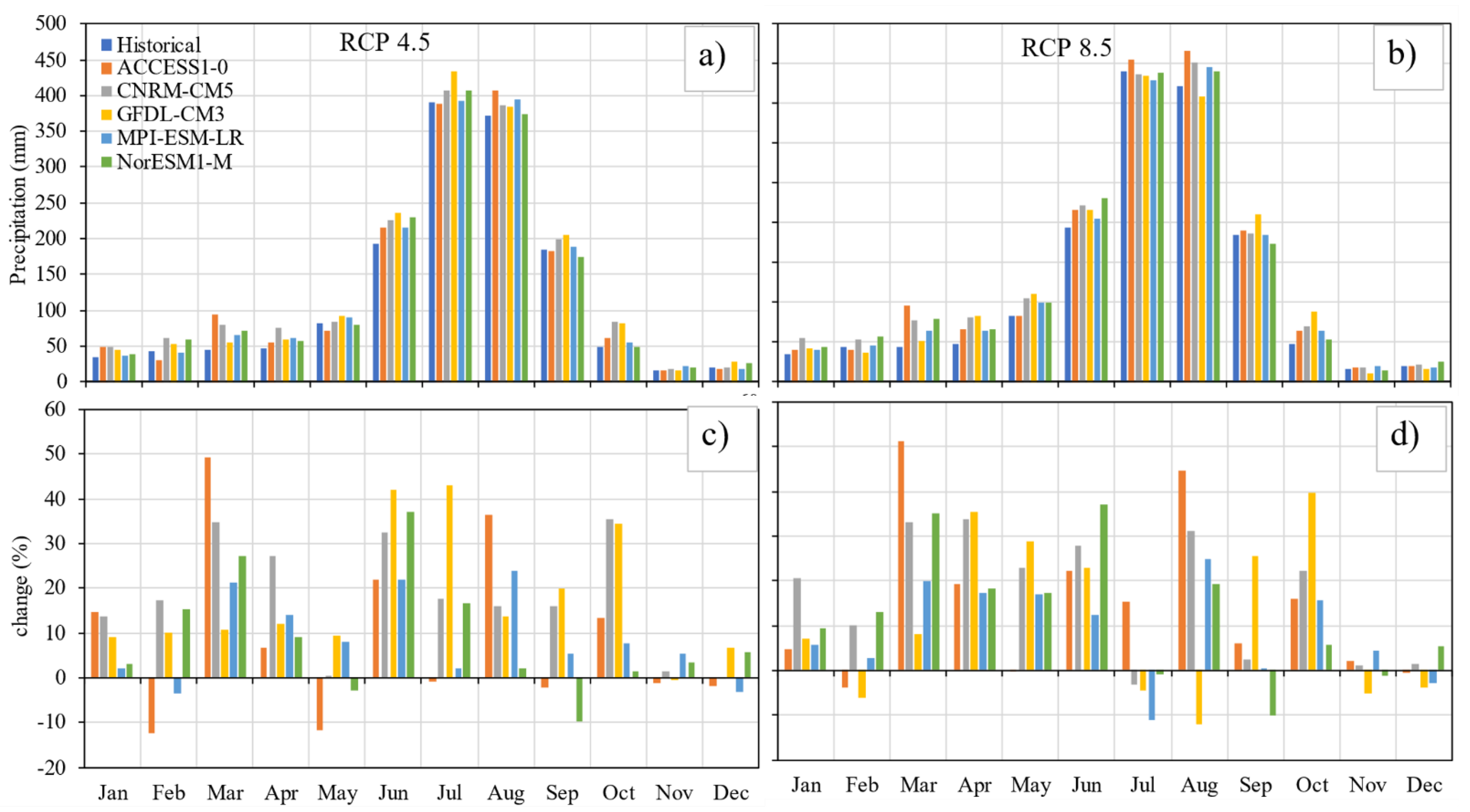
3.2. Projection and Changes in Monthly Precipitation

The monthly projection and percentage change in precipitation using multiple climate models under two RCP scenarios in the TBRB are shown in Figure 3. The average precipitation in the basin is projected to vary from 14.9 mm (ACCESS1-0) in November to 433.1 mm (GFDL-CM3) in July under RCP 4.5 (Figure 3a). Similarly, under RCP 8.5, the monthly precipitation is projected to vary from 10.8 mm (GFDL-CM3) in November to 415.8 mm (ACCESS1-0) in August (Figure 3b). Under RCP 4.5 and 8.5 the ACCESS1-0 climate model overestimated the precipitation projection in January, March, June, August, and October and underestimated the rest of the months. In contrast, the projected precipitation results from the CNRM-CM5 climate model showed an underestimation in December under RCP 4.5 and an underestimation in July and December under RCP 8.5. Similarly, an underestimation in precipitation projection was observed in November, February, and September and May as projected by GFDL-CM3, MPI-ESM-LR, and NorESM1-M, respectively, and an overestimation during the remaining months. In contrast, under RCP 8.5, the CNRM-CM5 climate model showed an underestimation in February, July, August, November, and December, and MPI-ESM-LR and NorESM1-M showed an underestimation in July and December and July, September, and November, respectively.

The highest (+49.3%) and lowest (−12.4%) change in projected precipitation was observed in March and February, respectively, under RCP 4.5 as projected by the ACCESS1-0 climate model (Figure 3c). Under RCP 8.5, the maximum change in the projected precipitation was found to be +51.1%, and the minimum change was found to be −11.9%, as depicted by ACCESS1-0 and GFDL-CM3 (Figure 3d). The greatest monthly precipitation shift was found to be +149.9% and +192.4% at station 418 and station 404 under RCP 4.5 and RCP 8.5, respectively. Similarly, the minimum change in monthly precipitation was found to be −41.9% and −44.9% at station 404 and station 303 under RCP 4.5 and RCP 8.5, respectively (

Table 3. The maximum and minimum shift in precipitation and temperature projection values at various stations under different climatic scenarios in the Thuli Bheri River Basin. The ‘+’ sign indicates the overestimation, and the ‘−‘ sign indicates the underestimation. The values within parentheses represent the respective values in percentage (%).

Station Name	RCP 4.5		RCP 8.5		Remarks
	Maximum Change	Minimum Change	Maximum Change	Minimum Change
Station 303	+44.9 mm (+89.6%)	−9.6 mm (−22.1%)	+15.1 mm (+97.5%)	−4.8 mm (−44.9%)	Precipitation
Station 304	+37.7 mm (+91.1%)	−9.1 mm (−27.0%)	+12.3 mm (+112.7%)	−2.2 mm (−20.6%)
Station 404	+42.8 mm (+133.6%)	−17.6 mm (−41.9%)	+61.6 mm (+192.4%)	−5.1 mm (−36.0%)
Station 418	+72.7 mm (+149.9%)	−19.3 mm (−32.3%)	+70.3 mm (+144.8%)	−7.8 mm (−37.3%)
Station 501	+48.7 mm (+123.8%)	−5.7 mm (−32.1%)	+54.3 mm (+138.1%)	−7.5 mm (−42.6%)
Station 303	+5.9 °C (+39.6%)	−3.4 °C (−14.3%)	+7.3 °C (+53.6%)	−2.6 °C (−10.7%)	Maximum Temperature
Station 513	+4.6 °C (+22.5%)	−11.1 °C (−32.2%)	+7.2 °C (+35.4%)	−11.1 °C (−32.2%)
Station 303	+3.7 °C (+20.8%)	+0.6 °C (+3.1%)	+5.8 °C (+30.7%)	+1.5 °C (+6.1%)	Minimum Temperature
Station 513	+2.3 °C (+11.5%)	−0.4 °C (+1.3%)	+4.9 °C (+16.9%)	+1.1 °C (+4.0%)

). The maximum change in the precipitation projection at station 418 and station 404 under RCP 4.5 and RCP 8.5 was projected to occur in March and April, respectively, while the minimum change in the precipitation projection was projected to occur in February and November under RCP 4.5 and RCP 8.5, respectively. Results of the precipitation projection and their changes show an underestimation in low flow months and overestimation in high flow months.

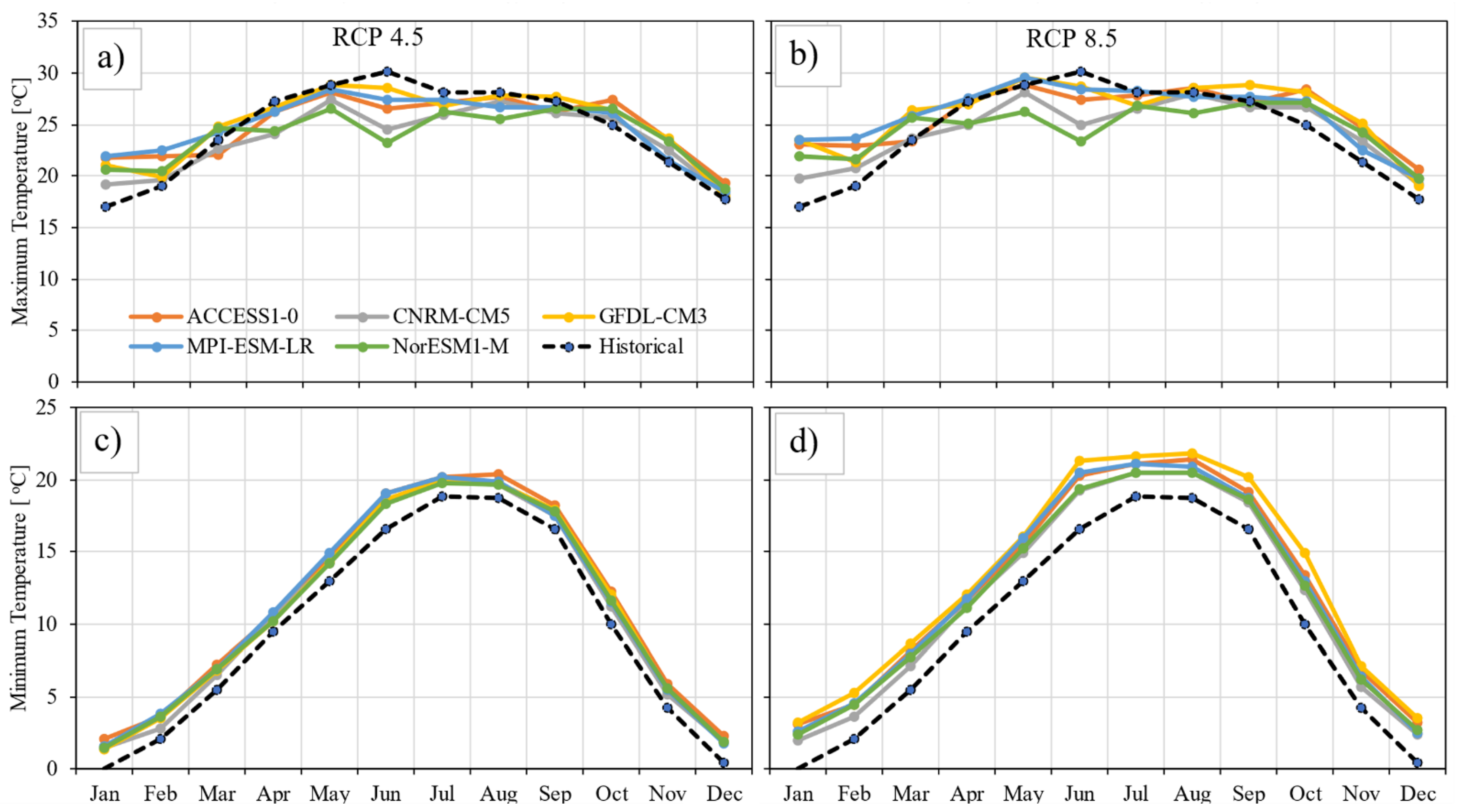
3.3. Projection and Changes in Monthly Temperature

The projection and changes in average monthly maximum and minimum temperature are shown in Figure 4. The monthly projection in average maximum temperature showed both overestimation and underestimation by the climate models (Figure 4a,b). The drier months (October to February) showed the overestimation in maximum temperature projection, and the wetter months (March to September) showed the underestimation in the maximum temperature projection, which implies that summer temperature is projected to reduce, and the winter temperature is projected to increase in the future. The monthly projection in average minimum temperature showed an overestimated temperature projection when using all the climate models (Figure 4c,d). The change in projected average maximum temperature varied from −6.9 °C (NorESM1-M) to +4.9 °C (MPI-ESM-LR) under RCP 4.5 and vary from −6.7 °C (NorESM1-M) to +6.6 °C (GFDL-CM3) under RCP 8.5. Similarly, the projection in average minimum temperature varied from +0.7 (NorESM1-M) to +2.5 °C (ACCESS1-0) under RCP 4.5 and from +1.4 (CNRM-CM5) to 4.9 °C (GFDL-CM3) under the RCP 8.5 climatic scenario. The minimum and maximum changes in average maximum temperature are projected to occur in June and January, respectively. At the same time, the change in average minimum temperature is projected to occur in February and June, respectively, under RCP 4.5. Under RCP 8.5, the minimum and maximum changes in average maximum temperature are projected to occur in June and January. These changes in average minimum temperature are projected to occur in November and October, respectively.

The station-wise absolute and relative change distribution of minimum and maximum change in both maximum and minimum temperature are shown in Table 3. At station 303, the relative change in the maximum and minimum value of maximum temperature was found to be +5.9 °C (ACCESS1-0) and −3.4 °C (NorESM1-M) under RCP 4.5 and +7.3 °C (MPI-ESM-LR) and −2.6 °C (NorESM1-M) under RCP 8.5. Similarly, the relative change in minimum temperature at the same station is projected to be +3.7 °C (MPI-ESM-LR) and +0.6 °C (CNRM-CM5) under RCP 4.5 and +5.8 °C (GFDL-CM3) and +1.5 °C (NorESM1-M) under RCP 8.5 climatic.

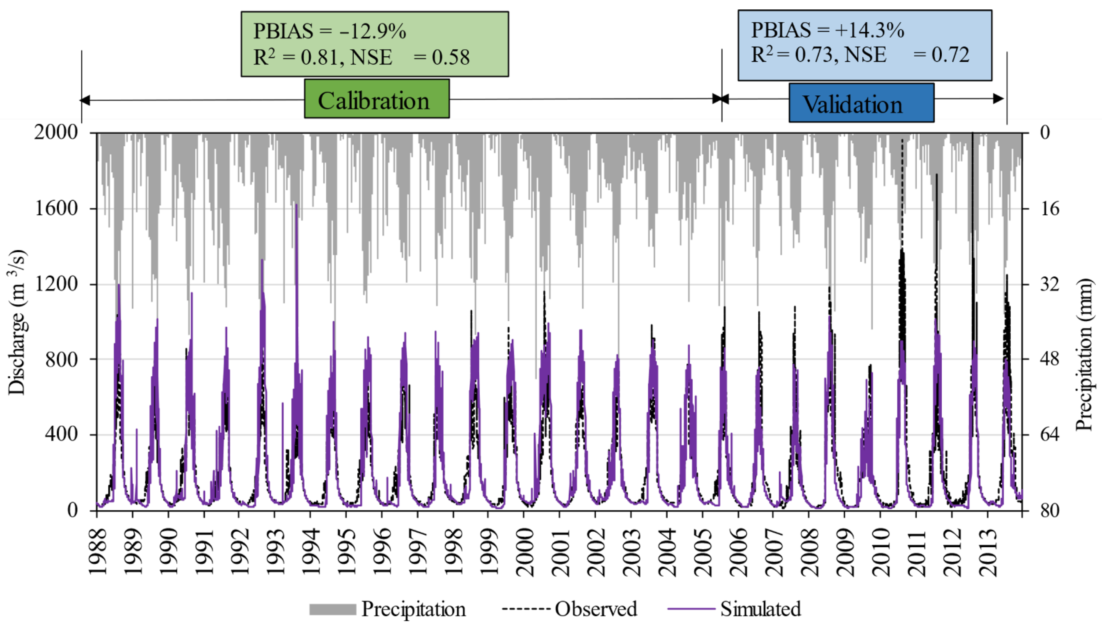
3.4. Calibration and Validation of SWAT Hydrological Model

The developed SWAT hydrological model for the TBRB was calibrated and validated for 1988–2006 and 2007–2013, respectively, as shown in Figure 5. The black dotted line represents observed daily discharge data. The solid purple line represents the simulated daily discharge data at Rimma gauge station. The grey vertical bar represents the average daily precipitation in the basin. Three statistical indicators, percentage bias (PBIAS), coefficient of determination (R²), and Nash–Sutcliffe efficiency (NSE), were observed to be −12.9%, 0.81, 0.58 for calibration, and +14.3%, 0.73, 0.72 for validation, respectively. Model performance can be considered satisfactory at PBIAS within ±25%, R² greater than 0.6, and NSE greater than 0.5 [42]. Thus, the statistical indicators showed the justifiable performance of model calibration and validation for the TBRB. During the simulation of the SWAT model, 20 sets of parameters were used, out of which 12 were found to be more sensitive towards observed discharge data. The parameters used in this study are tabulated in

Table 4. Parameters, their fitted value, and mode of changing the parameters used in the SWAT modeling.

Parameter Name	Description	Fitted Value	Change Method
SOL_K	Saturated hydraulic conductivity (mm/h)	−0.1	Multiply
CN2	SCS runoff curve number	−0.38	Multiply
SOL_AWC	Available water capacity of the soil layer (mm H2O/mm)	0.06	Multiply
GWQMN	Threshold depth of water in a shallow aquifer	3500	Replace
REVAPMN	Threshold depth if water in a shallow aquifer for revap	30	Replace
GW_REVAP	Groundwater revap coefficeient	0.2	Replace
RECHRG_DP	Deep aquifer percolation factor	0.15	Replace
GW_DELAY	Groundwater delay time (days)	100	Replace
ESCO	Soil evaporation compensation factor	0.5	Multiply
EPCO	Plant water uptake compensation factor	0.3	Replace
ALPHA_BF	Baseflow alpha factor	0.08	Replace
SURLAG	Surface runoff lag coefficient (days)	2.5	Replace
SNOCOVMX	Snow water equivalent to 100% snow cover (mm)	93.03	Replace
SNO50COV	Snow water equivalent to 50% snow cover (mm)	0.62	Replace
TLAPS	Temperatuure lapse rate (°C/km)	−6.3	Replace
PLAPS	Rainfall lapse rate (mm/km)	−170	Replace
SFTMP	Snowfall temperature [°C]	1.0	Replace
SMTMP	Snow melt base temperature [°C]	0.5	Replace
SMFMX	Melt factor for snow on June 21 [mm H2O/°C-day]	4.5	Replace
SMFMN	Melt factor for snow on December 21 [mm H2O/°C-day]	4.5	Replace

.

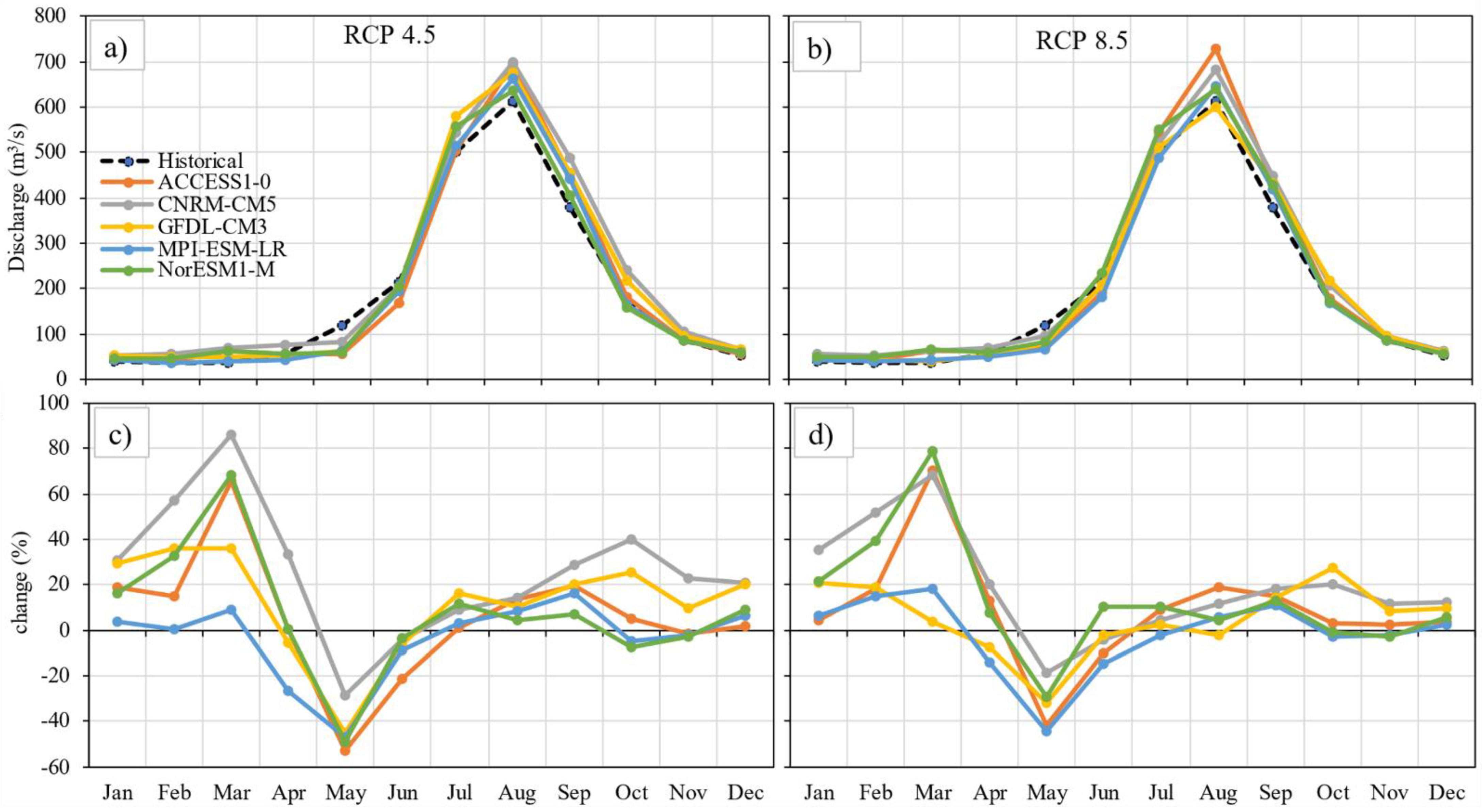
3.5. Projection and Changes in Monthly Streamflow

The projection and changes in average monthly streamflow using multiple climate models under RCP 4.5 and RCP 8.5 are shown in Figure 6. Under RCP 4.5, the streamflow projection is anticipated to vary from 35.9 m³/s to 699.4 m³/s as shown by MPI-ESM-LR and CNRM-CM5 climate models, respectively. Similarly, the streamflow projection under RCP 8.5 ranges from 38.7 m³/s to 728.7 m³/s as depicted by GFDL-CM3 and ACCESS1-0 climate models, respectively. The minimum streamflow projection is projected to occur in February under RCP 4.5 and in March under RCP 8.5. In contrast, the maximum streamflow projection is anticipated in August under RCP 4.5 and RCP 8.5 (Figure 6a,b). Further, the results portray an underestimation in low flow months and an under- and overestimation in high flow months in both climatic scenarios, which implies that the basin is projected to have heavy floods in high flow months and drought conditions in low flow months attenuated by fluctuations in precipitation and temperature patterns.

All the climate models showed an overestimated streamflow projection from July to March and an underestimated streamflow projection from May to June under RCP 4.5 and 8.5, respectively. However, a mixed tendency of overestimation and underestimation is observed by different climate models in April. GFDL-CM3 and MPI-ESM-LR projected an underestimation in streamflow simulation under both climatic scenarios, while ACCESS1-0, CNRM-CM5, and NorESM1-M projected an overestimated streamflow. Small traces (0.3 to 0.5%) of changes in streamflow are observed as shown by ACCESS1-0 and NorESM1-M under RCP 4.5. The results show that the minimum and maximum changes in streamflow projection are −62.4 mm (52.9%) and +32.1 mm (85.9%) under RCP 4.5. ACCESS1-0 projects the minimum change in streamflow to occur in May. In contrast, the maximum change in streamflow is projected by CNRM-CM5 in March. Under RCP 8.5, the minimum and maximum streamflow change are −52.5 mm (−44.5%) and +29.4 mm (+78.7%), respectively. The minimum and maximum changes in streamflow are projected by MPI-ESM-LR and NorESM1-M in May and March, respectively (Figure 6c,d).

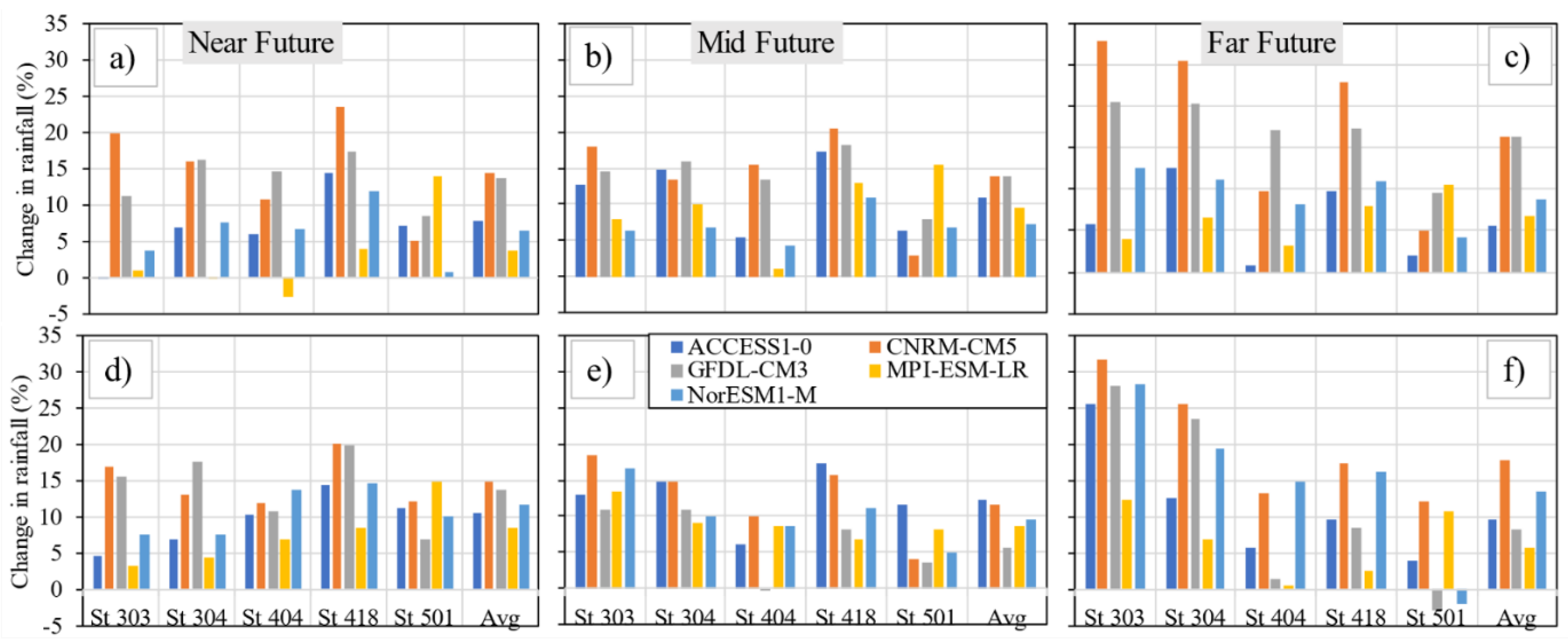
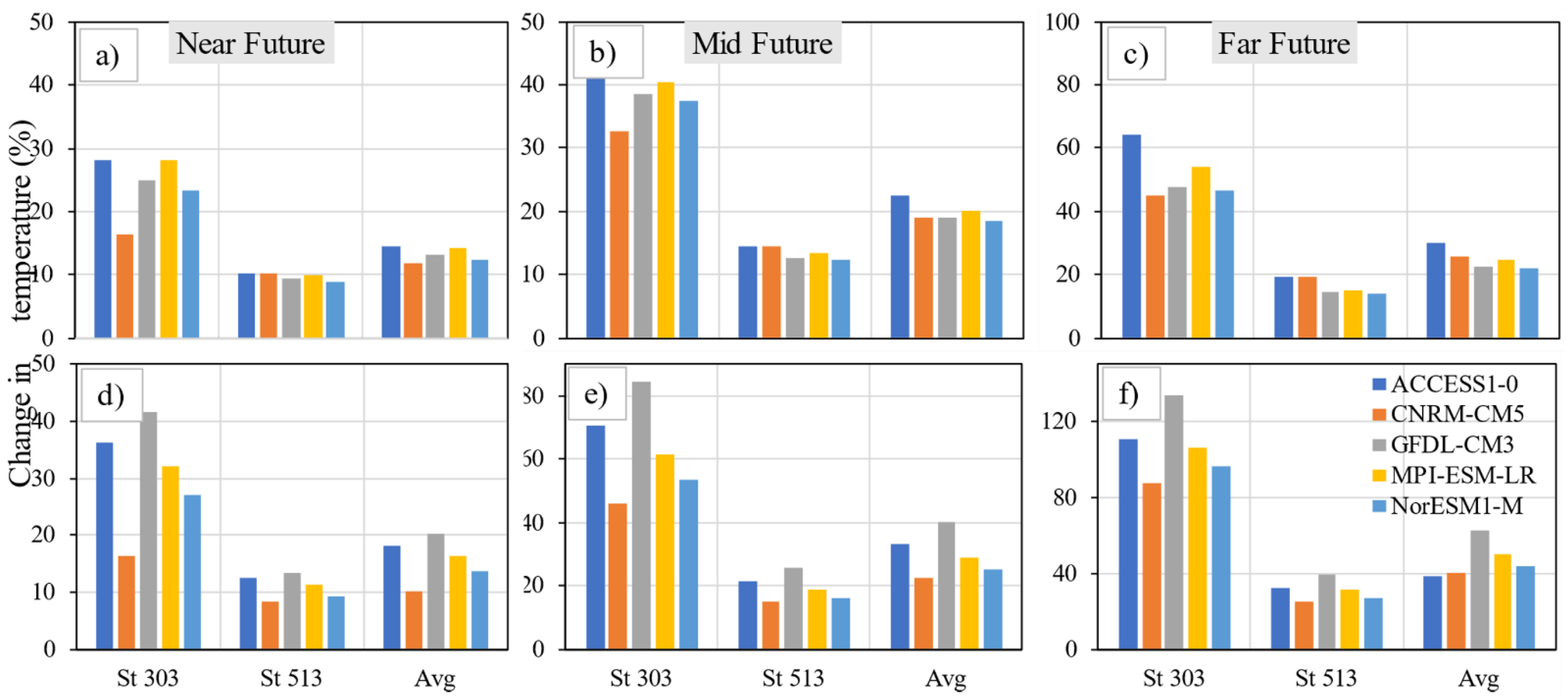
3.6. Projection and Changes in Precipitation Pattern for Future Time Windows

The projection and changes in precipitation pattern for three future time windows are shown in Figure S2 and Figure 7, respectively, under RCP 4.5 and RCP 8.5 emission scenarios. The projection in the precipitation pattern for three future time windows ranges from 818.8 mm (ACCESS1-0) to 2376.1 mm (CNRM-CM5) in Near Future, 884.2 mm (MPI-ESM-LR) to 2318.6 mm (CNRM-CM5) in Mid Future, and 852.4 mm (MPI-ESM-LR) to 2362.2 mm (CNRM-CM5) in Far Future under RCP 4.5. Under RCP 8.5, the projected precipitation in the basin is found to vary from 846.0 mm (MPI-ESM-LR) to 2308.8 mm (CNRM-CM5) in Near Future, 925.8 mm (ACCESS1-0) to 2257.8 mm (ACCESS1-0) in Mid Future, and 920.0 mm (MPI-ESM-LR) to 2258.3 mm (CNRM-CM5) in the Far Future. The spatial distribution of the precipitation pattern shows that the maximum amount of precipitation is projected to occur at Station 418, and the minimum is projected to occur at Station 303 under both climatic scenarios. Similarly, the basin average of the projected precipitation showed the variation in precipitation amount from 1528.2 mm (MPI-ESM-LR) to 1687.8 mm (CNRM-CM5) in Near Future, 1579.9 mm (NorESM1-M) to 1678.1 mm (GFDL-CM3) in Mid Future, and 1556.8 mm (ACCESS1-0) to 1714.1 mm (FGDL-CM3) in Far Future under RCP 4.5. Likewise, under RCP 8.5, the projection in basin average precipitation distribution varied from 1598.2 mm (MPI-ESM-LR) to 1692.2 mm (CNRM-CM5) in Near Future, 1558.3 mm (GFDL-CM3) to 1656.0 mm (ACCESS1-0) in Mid Future, and 1557.5 mm (MPI-ESM-LR) to 1737.1 mm (CNRM-CM5) in Far Future. The projection of the precipitation distribution is overestimated by all the considered climate models against the basin average observed precipitation (1474.2 mm), which signifies the plausible risk of heavy rains and floods in the future.

The absolute changes in the precipitation distribution for three future time windows vary from −2.8% to +23.5%, +1.1% to +20.5%, and +0.9% to +22.8% in Near Future, Mid Future, and Far Future, respectively, under RCP 4.5. The changes in the future precipitation pattern fluctuate from +3.2% to +20.0%, 0.0% to +18.4%, and −2.8% to +31.6% in Near Future, Mid Future, and Far Future, respectively. Under RCP 4.5, the lowest and highest change in the precipitation projection are projected by MPI-ESM-LR and CNRM-CM5 in Near Future, respectively. Similarly, the precipitation projection in Mid Future shows the maximum and minimum changes when using MPI-ESM-LR and CNRM-CM5 climate models, respectively. In contrast, the climate models ACCESS1-0 and CNRM-CM5 projected the minimum and maximum changes in precipitation occurrence in the Far Future. This states that uncertainty exists in the projection of future precipitation [4]. MPI-ESM-LR and CNRM-CM5 climate models exhibit the minimum and maximum changes in the future precipitation projection during Near Future, and GFDL-CM3 and CNRM-CM5 climate models during Mid and Far Future. The absolute and relative changes in the projected precipitation in three future periods are heterogeneous in spatial distribution under both emission scenarios. Under RCP 4.5, the lowest and highest variability in the projected precipitation are found at Stations 404 and 418 in Near, Mid, and Far Future, respectively. The spatial distribution at precipitation gauge stations shows the lowest alteration in Station 303 and the highest alteration in Station 418 in Near Future. Stations 404 and 303 exhibited the lowest and highest fluctuations in projected precipitation in Mid Future, and Stations 501 and 303 in Far Future under RCP 8.5. The non-homogenous projection of the precipitation pattern in temporal and spatial extent will eventually impact the water-related activities, such as agricultural yield, hydropower generation, hydropower generated economic development, and many more in the basin.

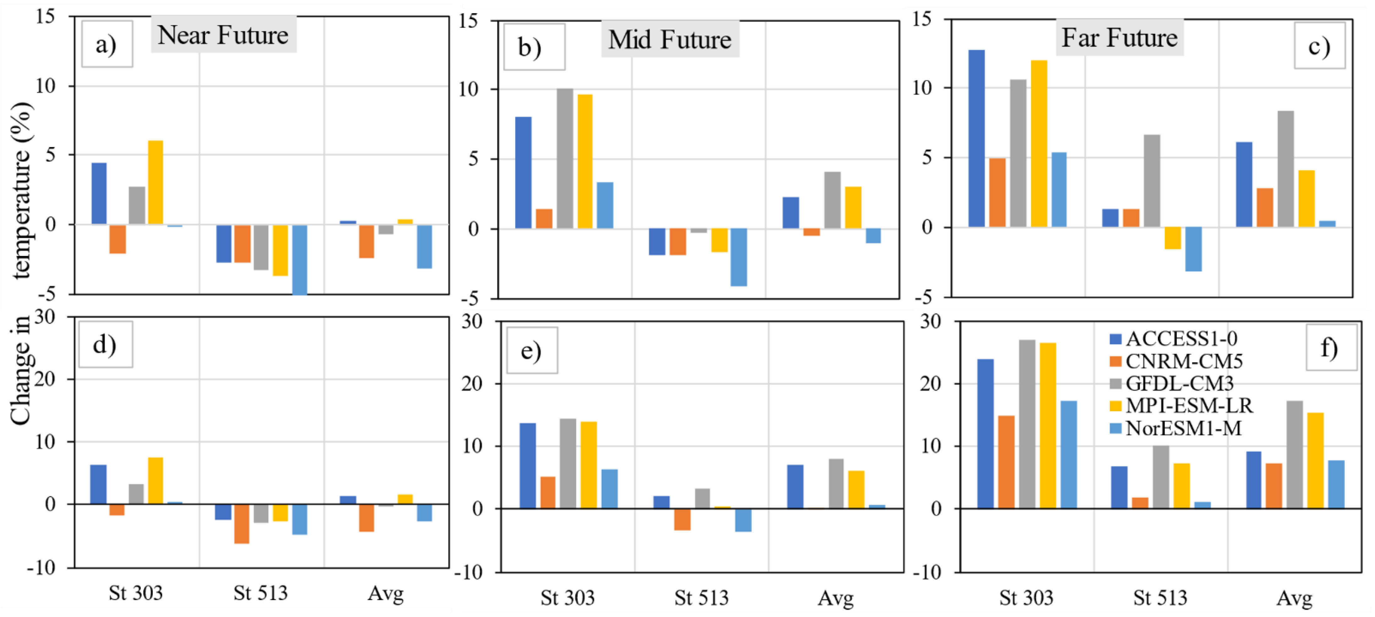
3.7. Projection and Changes in Temperature Pattern for Future Time Windows

The projections of maximum and minimum temperature (Figures S3 and S4) and their changes in percentage for future time windows under RCPs 4.5 and 8.5 (Figure 8 and Figure 9) show the increase in temperature on average. The future maximum temperature in the basin varied from 19.9 (CNRM-CM5) to 27.5 (ACCESS1-0 and CNRM-CM5) °C in Near Future, 20.6 (CNRM-CM5) to 28.2 (GFDL-CM3) °C in Mid Future, and 21.4 (CNRM-CM5) to 30.1 (GFDL-CM3) °C in Far Future under RCP 4.5 (Figure S2a–c). The projected maximum temperature in the basin is projected to vary from 20.0 (CNRM-CM5) to 27.6 (ACCESS1-0) °C in Near Future, 21.4 (CNRM-CM5) to 29.2 (GFDL-CM3) °C in Mid Future, and 23.4 (CNRM-CM5) to 31.2 (GFDL-CM3) °C in Far Future under RCP 8.5 (Figure S3d–f). Results of maximum temperature projection show an underestimation in Near Future and an overestimation in the Mid and Far Future, which indicates that the basin will have more heat events. The increase in heat events would have a potential impact on the regional hydrological cycle. Additionally, this will further increase the rate of evaporation and unconventional precipitation pattern in the basin. An increase in the maximum temperature would significantly impact biotic activities. Similarly, projection of the minimum temperature in the basin shows a variation from 5.3 (CNRM-CM5) to 15.7 (ACCESS1-0, CNRM-CM5, and MPI-ESM-LR) °C in Near Future, 6.0 (CNRM-CM5) to 16.3 (ACCESS1-0 and CNRM-CM5) °C in Mid Future, and 6.6 (CNRM-CM5) to 17.0 (ACCESS1-0 and CNRM-CM5) °C in Far Future under RCP 4.5 (Figure S3a–c). The projection in minimum temperature in the basin varied from 5.3 (CNRM-CM5) to 16.2 (GFDL-CM3) °C in Near Future, 6.7 (CNRM-CM5) to 17.9 (GFDL-CM3) °C in Mid Future, and 8.5 (CNRM-CM5) to 19.9 (GFDL-CM3) °C under RCP 8.5 (Figure S3d–f). The basin average maximum temperature in the basin is projected to fluctuate from 23.6 to 24.4 °C in Near Future, 24.2 to 25.3 °C in Mid Future, and 24.4 to 26.3 °C in Far Future under RCP 4.5. Under RCP 8.5, the basin average maximum temperature demonstrated a variation from 23.3 to 24.7 °C in Near Future, 24.4 to 26.3 °C in Mid Future, and 26.1 to 28.5 °C in Far Future. The projected average minimum temperature in the basin shows variations ranging from 10.6 to 10.8 °C in Near Future, 11.1 to 11.5 °C in Mid Future, and 11.5 to 12.3 °C in Far Future under RCP 4.5. The average projected minimum temperature in the basin varied from 10.4 to 11.1 °C in Near Future, 11.5 to 13.2 °C in Mid Future, and 13.0 to 15.3 °C in Far Future under RCP 8.5 (Figure S4).

The relative change in projected maximum temperature shows a reducing tendency in Near Future and an increasing tendency in the Mid and Far Future (Figure 8) under both emission scenarios. The relative change in station-based maximum temperature is found to vary from −5.3% (NorESM1-M) to +6.0% (MPI-ESM-LR) in Near Future, −4.2% (NorESM1-M) to +10.0% (GFDL-CM3) in Mid Future, and −3.2% (NorESM1-M) to +12.8% (ACCESS1-0) in Far Future under RCP 4.5 (Figure 8a–c), whereas under RCP 8.5, it vary from −6.2% (CNRM-CM5) to +7.6% (MPI-ESM-LR) in Near Future, −3.5% (NorESM1-M) to +14.6% (GFDL-CM3) in Mid Future, and +1.2% (NorESM1-M) to 27.0% (GFDL-CM3) in Far Future (Figure 8d–f). The minimum change in maximum temperature is pronounced at Station 513 (elevation: 910 masl), and the maximum change is pronounced in Station 303 (elevation: 2300 masl) for all future time windows under both climatic scenarios. High variation in maximum temperature is projected to occur in the high elevation area (northern belt of the basin). Less variation is projected to occur in the low elevation area (southern belt of the basin). The large increase in the maximum temperature will have a potential impact on surface water availability. An increase in flood events and drought events might be witnessed with an increase in maximum temperature. The increase in maximum temperature (Station 303) in the snow-fed region of the basin might melt the summer snow and increase the glacier flow as surface water with increased flood events. In contrast, the increased temperature will accelerate evaporation, increasing the dryness of the landmass.

The relative change in the minimum temperature for three future time windows is shown in Figure 9. Results of the projection of minimum temperature show an increasing tendency for all future time windows. The change is found to vary from +9.0% (NorESM1-M) to 28.1% (ACCESS1-0 and MPI-ESM-LR) in Near Future, +12.3% (NorESM1-M) to +47.2% (ACCESS1-0) in Mid Future, and +14.0% (NorESM1-M) to 64.1% (ACCESS1-0) in Far Future under RCP 4.5 (Figure 9a–c). Similarly, the change is witnessed to vary from +8.3% (CNRM-CM5) to +41.6% (GFDL-CM3) in Near Future, +14.8% (CNRM-CM5) to +84.5% (GFDL-CM3) in Mid Future, and +25.2% (CNRM-CM5) to +133.4% (GFDL-CM3) in Far Future (Figure 9d–f). The research results revealed that the basin average minimum temperature alteration fluctuates from +11.8 to 14.6% in Near Future, +18.4 to 22.4% in Mid Future, and +21.9 to 30.2% in Far Future. Further, the basin average minimum temperature is found to vary from +10.2 to +20.3% in Near Future, +22.3 to 33.4% in Mid Future, and +38.6 to 62.1% in Far Future under RCP 8.5. The results portray a relatively large increase in the projected minimum temperature in Mid and Far Future periods, which might significantly impact different components of the hydrological cycle of the basin. Similar to maximum temperature, the skyrocketing increase in the minimum temperature might be responsible for increased climatic hazards, such as heatwaves, dry days, and drought events in the future.

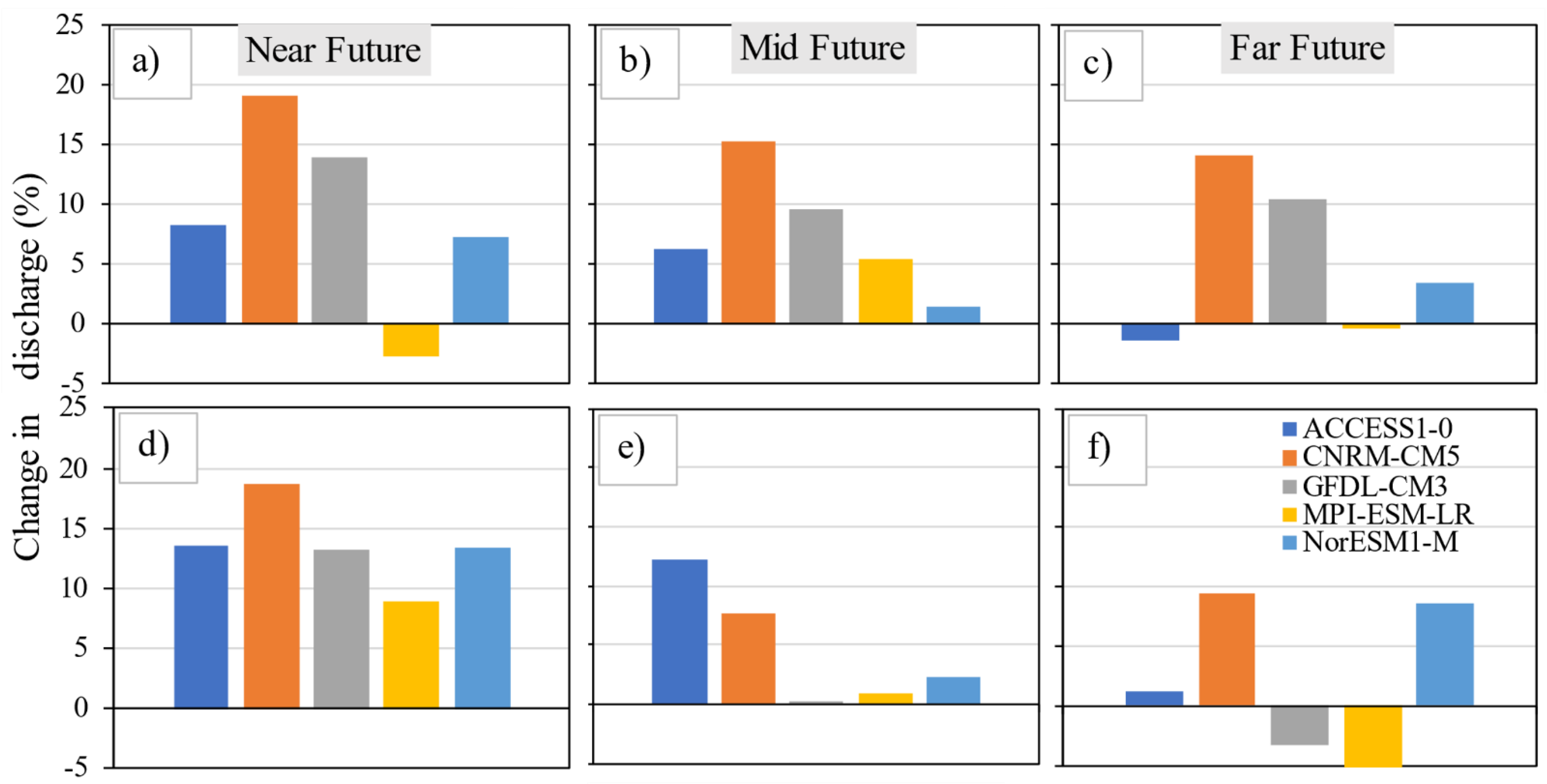
3.8. Projection and Changes in Streamflow Pattern for Future Time Windows

The projection and changes in the future streamflow measured at the Rimma gauge station are shown in Figure S5 and Figure 10. The projected result shows a variation in streamflow from 188.8 m³/s (MPI-ESM-LR) to 231.1 m³/s (CNRM-CM5) in Near Future, 196.9 m³/s (NorESM1-M) to 223.6 m³/s (CNRM-CM5) in Mid Future, and 191.4 m³/s (ACCESS1-0) to 221.4 m³/s (CNRM-CM5) in Far Future under RCP 4.5 (Figure S5a–c). The streamflow at the gauge station varied from 211.3 m³/s (MPI-ESM-LR) to 230.3 m³/s (CNRM-CM5) in Near Future, 194.5 m³/s (GFDL-CM3) to 217.7 m³/s (ACCESS1-0) in Mid Future, and 176.2 m³/s (MPI-ESM-LR) to 212.5 m³/s (CNRM-CM5) in Far Future under RCP 8.5 (Figure S5d–f). The projected result shows increased streamflow in the Near and Mid Future and decreased streamflow in the Far Future by some models. MPI-ESM-LR projected the reduced streamflow in the Near Future, and ACCESS1-0 and MPI-ESM-LR in the Far Future under RCP 4.5. In contrast, under RCP 8.5, GFDL-CM3 and MPI-ESM-LR projected reduced streamflow only in the Far Future. The other models projected an increase in the future streamflow under both RCPs.

The change in projected streamflow varied from −2.7% to +19.1% in Near Future, +1.5 to +15.2% in Mid Future, and −0.4% to +14.1% in Far Future under RCP 4.5 (Figure 10a–c). In contrast, the relative change in the projected streamflow varied from +8.8 to +18.6% in Near Future, +0.2 to +12.2% in Mid Future, and −9.2 to +8.6% in Far Future under RCP 8.5 (Figure 10d–f). The maximum change in the streamflow is projected using the CNRM-CM5 climate model, and the minimum change is projected by the MPI-ESM-LR climate model in the Near Future under RCP 4.5. In contrast, in the Mid Future, NorESM1-M projected low streamflow, and CNRM-CM5 projected high streamflow. MPI-ESM-LR projected reduced streamflow, and CNRM-CM5 projected increased streamflow in the Far Future. The temporal variation of the projected streamflow shows a high value when using the CNRM-CM5 climate model and a low value when using the MPI-ESM-LR climate model in the Near Future. Compared to the Near Future, the climate model GFDL-CM3 projected low streamflow, and ACCESS1-0 climate model projected high streamflow in the Mid Future. In contrast to Near and Mid Future, underestimation in streamflow is projected by the MPI-ESM-LR climate model, and overestimation in streamflow is projected by the CNRM-CM5 climate model in the Far Future.

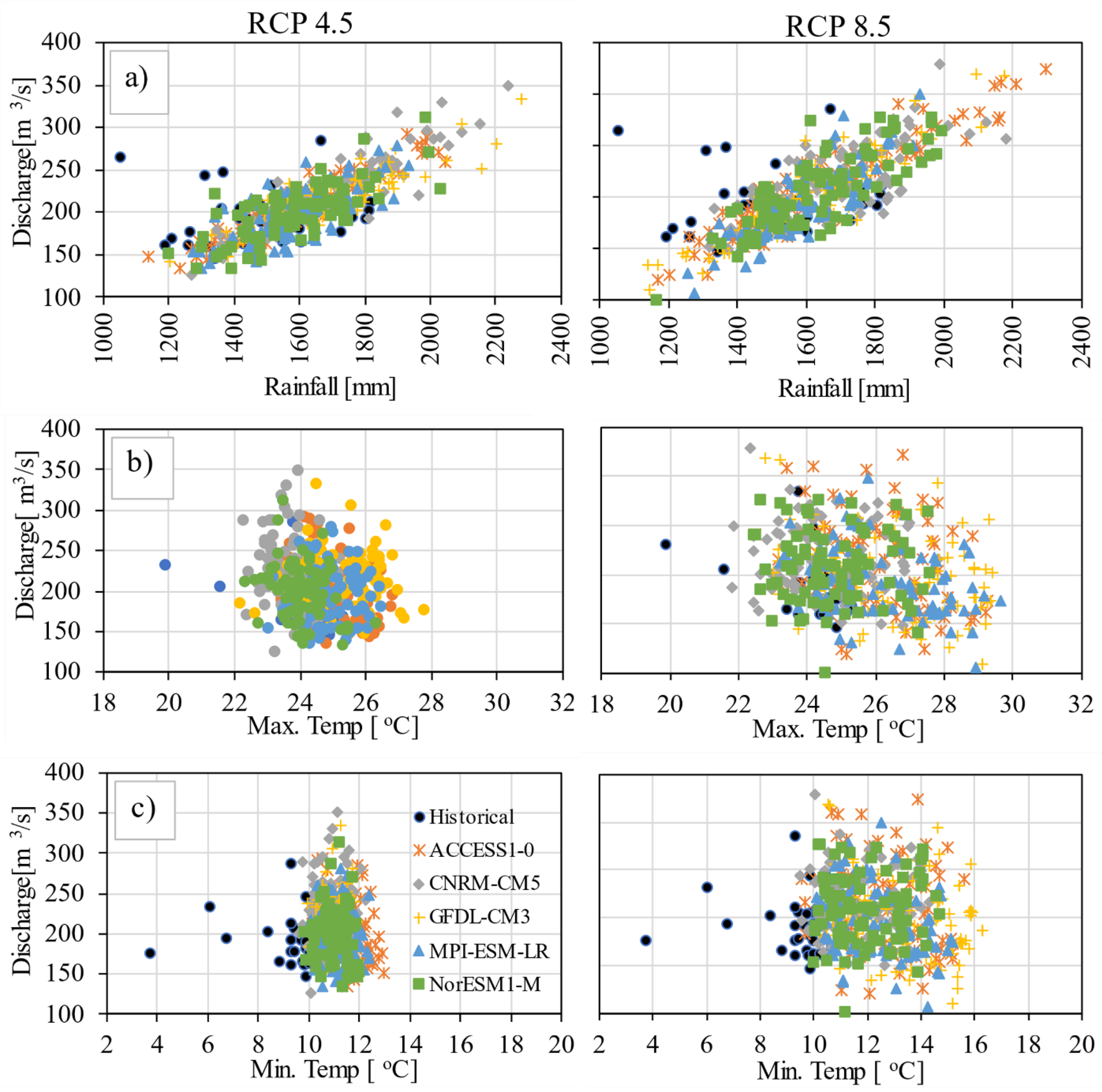
3.9. Relation between Precipitation, Temperature, and Streamflow

The scatter plot in Figure 11 shows the relation between precipitation, temperature, and streamflow for observed and projected events using multiple climate models. The coefficient of determination (R²) and the governing regression equation are shown in

Table 5. Coefficient of determination (R²) and governing regression equation to establish the relationship between precipitation, maximum temperature (Tmax), minimum temperature (Tmin) and streamflow.

Climate Models	Precipitation-Streamflow		Tmax-Streamflow		Tmin-Streamflow		Emission Scenario
	R2	Reg. Equation	R2	Reg. Equation	R2	Reg. Equation
Observed	0.006	0.0124x + 175.64	0.079	−7.698x + 379.12	0.003	−1.2092x + 203.34	Historical
ACCESS1-0	0.863	0.1753x − 75.104	0.232	−21.089x + 729.13	0.089	−15.141x + 376.70	RCP 4.5
CNRM-CM5	0.776	0.1851x − 88.705	0.042	−12.564x + 524.14	0.004	−4.3053x + 273.13
GFDL-CM3	0.802	0.1506x − 39.548	5 × 10−5	−0.226x + 220.55	0.006	−5.2209x + 272.88
MPI-ESM-LR	0.515	0.1573x − 52.339	0.002	+1.965x + 147.37	0.005	+4.0496x + 150.72
NorESM1-M	0.529	0.1444x − 28.840	0.065	−12.113x + 491.00	0.002	−3.0306c + 233.68
ACCESS1-0	0.876	0.1656x − 62.265	0.078	−8.4302x + 431.13	0.036	−5.9331x + 285.90	RCP 8.5
CNRM-CM5	0.523	0.1405x − 22.635	0.012	−3.243x + 294.35	0.000	−0.3233x + 218.37
GFDL-CM3	0.842	0.1806x − 90.913	0.098	−6.6536x + 375.23	0.089	−7.0859x + 293.84
MPI-ESM-LR	0.706	0.2083x − 137.99	0.135	−8.3592x + 411.21	0.104	−8.4461x + 297.08
NorESM1-M	0.644	0.1649x − 61.762	0.002	−1.1695x + 236.94	0.001	+0.6096x + 200.59

for 1981–2099. The observed data were plotted for 1981–2014 and the projected data for 2021–2099. The temporal relation between precipitation and streamflow is shown in Figure S6 for all the climate models under RCP 4.5 and RCP 8.5. The association between precipitation and streamflow indicates poor agreement for observed value while a medium to good agreement for projected value. The R² values varied from 0.515 (MPI-ESM-LR) to 0.863 (ACCESS1-0) under RCP 4.5, whereas under RCP 8.5, the R² value varied from 0.523 (CNRM-CM5) to 0.876 (ACCESS1-0). The linear regression between observed precipitation and streamflow shows that unit change in precipitation measured in the ‘mm’ unit will alter the streamflow by 0.0124 m³/s. A large variation in streamflow against the unit change in precipitation amount is projected to occur when predicting the river streamflow using CNRM-CM5 (0.1851 m³/s) under RCP 4.5 and using MPI-ESM-LR (0.2083 m³/s) under RCP 8.5. The results of the precipitation–streamflow relation reveal that the streamflow will increase substantially in the future compared to the historical trend, indicating that the basin may face frequent flash floods, increased runoff, and reduced groundwater recharge potential in the future. A large variation in the precipitation amount is predicted to widen variation in streamflow using ACCESS1-0 and CNRM-CM5 under RCP 4.5 and ACCESS1-0 under RCP 8.5. A medium-to-low streamflow is expected when NorESM1-M is considered in streamflow simulation, highlighting that the climate model shows uncertainty in the streamflow simulation [43,44]. An ensemble of various climate models can minimize the uncertainty in predicting future streamflow, which helps in efficient water resource management.

In terms of temperature, there is no significant change in streamflow with the temperature change. However, the linear regression equation showed a slight reduction in the streamflow with a unit increase in the maximum and minimum temperature for all the climate models, except MPI-ESM-LR under RCP 4.5 and NorESM1-M under RCP 8.5. The linear model predicts a rise in the streamflow by 1.965 m³/s and 4.0496 m³/s (MPI-ESM-LR), increasing maximum and minimum temperature by unit degree, respectively, under RCP 4.5. On the other hand, the model predicted a unit degree increase in minimum temperature would increase the streamflow by 0.6096m³/s (NorESM1-M) under RCP 8.5. Our results show that with an increase in temperature, the glaciers and snow of the basin will melt and result in increased streamflow.

4. Discussion

4.1. Projection and Changes in Precipitation, Temperature, and Streamflow

The results reveal an indication of hydro-climatic variability in TBRB in the future. The precipitation, temperature, and streamflow projection and their changes showed wide fluctuations in both monthly and annual temporal scales. The spatial and temporal average monthly projected precipitation varied from −12.4 to +49.3% under RCP 4.5 and −11.9 to +51.1% under RCP 8.5. The maximum temperature distribution varied from −6.9 to +4.9% under RCP 4.5 and −6.7 to +6.6% under RCP 8.5. Similarly, the minimum temperature distribution showed fluctuations ranging from +0.7 to +2.5% under RCP 4.5 and +1.4% to +4.9% under RCP 8.5. In contrast, the streamflow fluctuates from −52.9 to 85.9% under RCP 4.5 and −44.5 to +78.7% under RCP 8.5. The result showed that alteration in precipitation and temperature due to climate change has a significant impact on the streamflow of TBRB. Even a small precipitation elasticity will have a substantial impact on river streamflow generation [45]. The results outline that significant fluctuations in precipitation, temperature and streamflow are predicted to occur, which need serious attention. The results are congruent with other Nepalese and Indian river basins with similar topographic features [5,16,19,46,47].

The precipitation, temperature, and streamflow projection and their changes show the non-homogenous distribution in monthly and future time windows, which is analogous to other research carried out in the Koshi river basin [48]. The non-homogeneity in both space and time is shown by overestimation and underestimation of the projected precipitation, temperature, and streamflow. The underestimation and overestimation in the projected precipitation and temperature might be the consequences of various uncertainties associated with the climate models. At the same time, the fluctuation in the streamflow might be the result of the uncertainty attributed to the hydrological model and bias correction techniques [4,17]. Further, the variation in the temporal and spatial heterogeneity of the observed precipitation and temperature distribution is controlled by natural and anthropogenic activities. The basin’s geomorphology and natural landscape also impact the precipitation and temperature the basin receives. Depending on the spatio-temporal precipitation distribution and a land interception, the surface and sub-surface streamflow are controlled. The streamflow is low during the pre-monsoon season until the soil is supersaturated, even with heavy precipitation for the first few days. However, the ground is already saturated during the monsoon season, and the rain falling in the basin will flow as streamflow. Thus, future land use and land cover type might be a controlling factor for future streamflow besides precipitation and temperature.

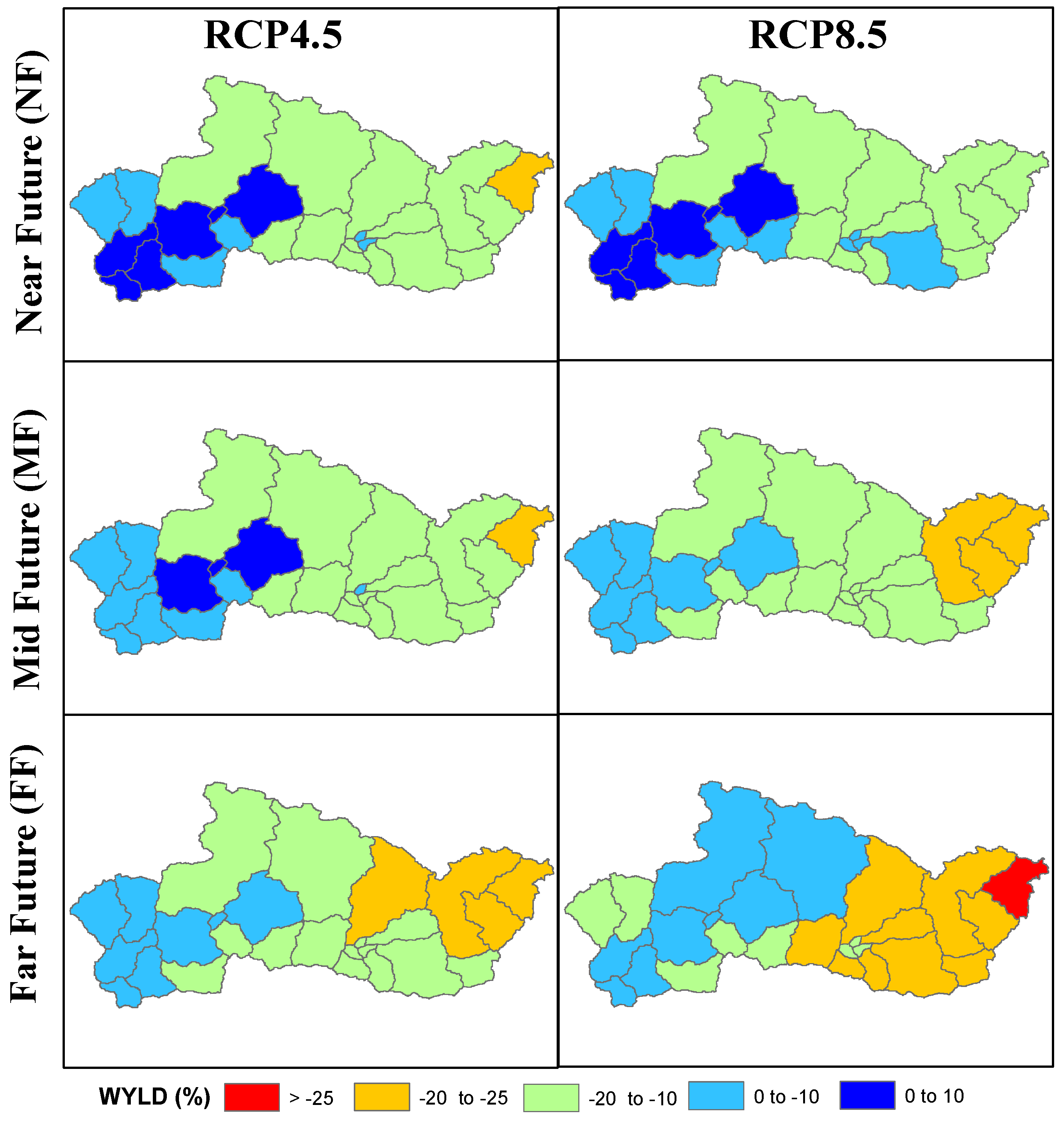
4.2. Impact of Climate Change on the Basin Water Yield

The changes in the water yield (WYLD) imposed by the changes in the projected precipitation and temperature pattern under RCP 4.5 and RCP 8.5 show a mixed tendency of increase and decrease in the spatial distribution of water yield in TBRB (Figure 12). The water yield varies from −28.4% in the east of the basin in the Far Future under RCP 8.5 to +5.4% towards the west in the Near Future under RCP 8.5. The monthly distribution of water yield is more during wet months (June–September) and less observed in dry months (October–May) in Himalayan basins [49,50]. The reduction in the water yield was reported by various pieces of research in Nepalese [5,19] and other river basins across the world [51,52]. The fluctuations in water yield in TBRB will eventually have an impact on the BBDMP. The increase in water yield ensures the project’s sustainability, while the reverse is the case when the water yield in the basin is reduced. The two basins (TBRB and BaRB) fall in two different provinces according to the new constitution of Nepal. This might create water disputes between the provincial governments with the increase or decrease of water yield in the TBRB. Further, the fluctuations in the water yield will also impact the future water-related projects in the TBRB and BaRB. Therefore, a major discussion on water distribution in the trans-boundaries is essential at national and provincial levels. Climatic and non-climatic factors attenuate the reduction in water yield. The climatic factors include precipitation and temperature, while the non-climatic elements include land use and cover change, soil type, basin slope, and many more [5].

5. Conclusions

The study used multiple climate models to assess the future projection and changes in the precipitation and temperature over TBRB in the Karnali Province, Nepal. Further, the study used the SWAT model to simulate the future streamflow under RCPs 4.5 and 8.5. Since the basin is snow-fed, the parameters controlling the snow were well-judged and calibrated in the SWAT model. The projected changes in the precipitation, temperature, and streamflow were evaluated using five RCMs under medium and high RCPs. The projected precipitation and temperature in the basin vary both temporally and spatially. The temporal projection shows that the precipitation fluctuates from −42 to +150% under RCP 4.5 and from −44 to 192% under RCP 8.5 for 2021–2100. The overestimation of the precipitation projection in high flow months suggests that the basin will receive more intense floods during these months. Similarly, the underestimated precipitation projection in low flow months highlights that the basin is at risk of drought conditions that will eventually impact the surface water availability and agricultural yield. Similarly, the projection and changes in the temperature show an increase in both minimum and maximum temperature. The temperature rise leads to the melting of the snow in the basin, resulting in flooding.

The spatial and temporal distribution of the water yield in the basin show the non-homogenous distributional impact of changing climate. The water yield in the basin is anticipated to alter from −28 to +5%. The reduction in the water yield and increase in the precipitation distribution suggests that the study area will likely receive short-duration precipitation leading to flash floods, which is one of the major findings of the research. The increased intensity of the flash floods will carry large sediments with it and might damage the infrastructure of BBMDP downstream. Further, increased sediment load will significantly impact agricultural productivity in the basin itself and downstream. In contrast, the reduced precipitation will lead to reduced streamflow, which might raise questions on the sustainability of the BBDMP. The reduced river water volume will eventually impact the hydropower generation and year-round irrigation of the BBMDP through the Babai Irrigation Project. This finding suggests that the basin needs to be addressed soon against the changing climate.

References

1. Pachauri, R.K.; Allen, M.R.; Barros, V.R.; Broome, J.; Cramer, W.; Christ, R.; Church, J.A.; Clarke, L.; Dahe, Q.; Dasgupta, P.; et al. Climate Change 2014: Synthesis Report. Contribution of Working Groups I, II and III to the Fifth Assessment Report of the IntergovernMental Panel on Climate Change; IPCC: Geneva, Switzerland, 2014; p. 151. [Google Scholar]
2. Jeuland, M.; Harshadeep, N.; Escurra, J.; Blackmore, D.; Sadoff, C. Implications of climate change for water resources development in the Ganges basin. Water Policy 2013, 15, 26–50. [Google Scholar] [CrossRef] [Green Version]
3. Taye, M.T.; Willems, P.; Block, P. Implications of climate change on hydrological extremes in the Blue Nile basin: A review. J. Hydrol. Reg. Stud. 2015, 4, 280–293. [Google Scholar] [CrossRef] [Green Version]
4. Aryal, A.; Shrestha, S.; Babel, M.S. Quantifying the sources of uncertainty in an ensemble of hydrological climate-impact projections. Theor. Appl. Climatol. 2019, 135, 193–209. [Google Scholar] [CrossRef]
5. Pandey, V.P.; Dhaubanjar, S.; Bharati, L.; Thapa, B.R. Spatio-temporal distribution of water availability in Karnali-Mohana Basin, Western Nepal: Climate change impact assessment (Part-B). J. Hydrol. Reg. Stud. 2020, 29, 100691. [Google Scholar] [CrossRef]
6. Arheimer, B.; Lindström, G. Climate impact on floods: Changes in high flows in Sweden in the past and the future (1911–2100). Hydrol. Earth Syst. Sci. 2015, 19, 771–784. [Google Scholar] [CrossRef] [Green Version]
7. Kalnay, E.; Cai, M. Impact of urbanization and land-use change on climate. Nature 2003, 423, 528–531. [Google Scholar] [CrossRef]
8. Collins, M.; Knutti, R.; Arblaster, J.; Dufresne, J.L.; Fichefet, T.; Friedlingstein, P.; Gao, X.; Gutowski, W.J.; Johns, T.; Krinne, G.; et al. Long-term climate change: Projections, commitments and irreversibility. In Climate Change 2013-The Physical Science Basis: Contribution of Working Group I to the Fifth Assessment Report of the Intergovernmental Panel on Climate Change; Cambridge University Press: Cambridge, UK; New York, NY, USA, 2013; pp. 1029–1136. [Google Scholar]
9. Meehl, G.A.; Stocker, T.F.; Collins, W.D.; Friedlingstein, P.; Gaye, A.T.; Gregory, J.M.; Kitoh, A.; Knutti, R.; Murphy, J.M.; Noda, A.; et al. Global Climate Projections. In Climate Change 2007: The Physical Science Basis. Contribution of Working Group I to the Fourth Assessment Report of the Intergovernmental Panel on Climate Change; Solomon, S.D., Qin, M., Manning, Z., Chen, M., Marquis, K.B., Averyt, M., Tignor, A.M., Miller, H.L., Eds.; Cambridge University Press: Cambridge, UK; New York, NY, USA, 2007; Available online: https://www.ipcc.ch/site/assets/uploads/2018/02/ar4-wg1-chapter10-1.pdf (accessed on 23 May 2021).
10. Kirtman, B.; Power, S.B.; Adedoyin, A.J.; Boer, G.J.; Bojariu, R.; Camilloni, I.; Doblas-Reyes, F.J.; Fiore, A.M.; Kimoto, M.; Meehl, G.A.; et al. Near-Term Climate Change: Projections and Predictability; Cambridge University Press: Cambridge, UK; New York, NY, USA, 2013. [Google Scholar]
11. Xin, X.; Zhang, L.; Zhang, J.; Wu, T.; Fang, Y. Climate change projections over East Asia with BCC_CSM1. 1 climate model under RCP scenarios. J. Meteorol. Soc. Jpn. Ser. II 2013, 91, 413–429. [Google Scholar] [CrossRef] [Green Version]
12. Tadross, M.; Jack, C.; Hewitson, B. On RCM-based projections of change in southern African summer climate. Geophys. Res. Lett. 2005, 32, 2393–2413. [Google Scholar] [CrossRef]
13. Khadka, D.; Pathak, D. Climate change projection for the Marsyangdi river basin, Nepal using statistical downscaling of GCM and its implications in geodisasters. Geoenviron. Disasters 2016, 3, 1–15. [Google Scholar] [CrossRef] [Green Version]
14. Devkota, L.P.; Gyawali, D.R. Impacts of climate change on hydrological regime and water resources management of the Koshi River Basin, Nepal. J. Hydrol. Reg. Stud. 2015, 4, 502–515. [Google Scholar] [CrossRef] [Green Version]
15. Kurihara, K.; Ishihara, K.; Sasaki, H.; Fukuyama, Y.; Saitou, H.; Takayabu, I.; Murazaki, K.; Sato, Y.; Yukimoto, S.; Noda, A. Projection of climatic change over Japan due to global warming by high-resolution regional climate model in MRI. Sola 2005, 1, 97–100. [Google Scholar] [CrossRef]
16. Dahal, P.; Shrestha, M.L.; Panthi, J.; Pradhananga, D. Modeling the future impacts of climate change on water availability in the Karnali River Basin of Nepal Himalaya. Environ. Res. 2020, 185, 109430. [Google Scholar] [CrossRef]
17. Shrestha, S.; Shrestha, M.; Babel, M.S. Modelling the potential impacts of climate change on hydrology and water resources in the Indrawati River Basin, Nepal. Environ. Earth Sci. 2016, 75, 1–13. [Google Scholar] [CrossRef]
18. Bajracharya, A.R.; Bajracharya, S.R.; Shrestha, A.B.; Maharjan, S.B. Climate change impact assessment on the hydrological regime of the Kaligandaki Basin, Nepal. Sci. Total Environ. 2018, 625, 837–848. [Google Scholar] [CrossRef]
19. Mishra, Y.; Nakamura, T.; Babel, M.S.; Ninsawat, S.; Ochi, S. Impact of climate change on water resources of the Bheri River Basin, Nepal. Water 2018, 10, 220. [Google Scholar] [CrossRef] [Green Version]
20. Oki, T.; Agata, Y.; Kanae, S.; Saruhashi, T.; Yang, D.W.; Musiake, K. Global assessment of current water resources using total runoff integrating pathways. Hydrol. Sci. J. 2001, 46, 983–995. [Google Scholar] [CrossRef] [Green Version]
21. Hanasaki, N.; Fujimori, S.; Yamamoto, T.; Yoshikawa, S.; Masaki, Y.; Hijioka, Y.; Kainuma, M.; Kanamori, Y.; Masui, T.; Takahashi, K.; et al. A global water scarcity assessment under shared socio-economic pathways–Part 2: Water availability and scarcity. Hydrol. Earth Syst. Sci. 2013, 17, 2393–2413. [Google Scholar] [CrossRef] [Green Version]
22. Guan, X.; Zhang, J.; Elmahdi, A.; Li, X.; Liu, J.; Liu, Y.; Jin, J.; Liu, Y.; Bao, Z.; Liu, C.; et al. The Capacity of the Hydrological Modeling for Water Resource Assessment under the Changing Environment in Semi-Arid River Basins in China. Water 2019, 11, 1328. [Google Scholar] [CrossRef] [Green Version]
23. Phan, T.T.H.; Sunada, K.; Oishi, S.; Sakamoto, Y. River streamflow in the Kone River basin (Central Vietnam) under climate change by applying the BTOPMC distributed hydrological model. J. Water Clim. Chang. 2010, 1, 269–279. [Google Scholar] [CrossRef] [Green Version]
24. Nazari-Sharabian, M.; Taheriyoun, M.; Ahmad, S.; Karakouzian, M.; Ahmadi, A. Water quality modeling of Mahabad Dam watershed–reservoir system under climate change conditions, using SWAT and system dynamics. Water 2019, 11, 394. [Google Scholar] [CrossRef] [Green Version]
25. Arnold, J.G.; Srinivasan, R.; Muttiah, R.S.; Williams, J.R. Large area hydrologic modeling and assessment part I: Model development 1. JAWRA 1998, 34, 73–89. [Google Scholar] [CrossRef]
26. Arnold, J.G.; Moriasi, D.N.; Gassman, P.W.; Abbaspour, K.C.; White, M.J.; Srinivasan, R.; Santhi, C.; Harmel, R.D.; Van Griensven, A.; Van Liew, M.W.; et al. SWAT: Model use, calibration, and validation. Trans. ASABE 2012, 55, 1491–1508. [Google Scholar] [CrossRef]
27. Cuceloglu, G.; Abbaspour, K.C.; Ozturk, I. Assessing the water-resources potential of Istanbul by using a soil and water assessment tool (SWAT) hydrological model. Water 2017, 9, 814. [Google Scholar] [CrossRef] [Green Version]
28. Abbaspour, K.C.; Rouholahnejad, E.; Vaghefi, B.; Srinivasan, R.; Yang, H.; Kløve, B. A continental-scale hydrology and water quality model for Europe: Calibration and uncertainty of a high-resolution large-scale SWAT model. J. Hydrol. 2015, 524, 733–752. [Google Scholar] [CrossRef] [Green Version]
29. Dhami, B.; Himanshu, S.K.; Pandey, A.; Gautam, A.K. Evaluation of the SWAT model for water balance study of a mountainous snowfed river basin of Nepal. Environ. Earth Sci. 2018, 77, 1–20. [Google Scholar] [CrossRef]
30. Bhatta, B.; Shrestha, S.; Shrestha, P.K.; Talchabhadel, R. Modelling the impact of past and future emission scenarios on streamflow in a highly mountainous watershed: A case study in the West Seti River Basin, Nepal. Sci. Total Environ. 2020, 740, 140156. [Google Scholar] [CrossRef]
31. Pokhrel, B.K. Impact of land use change on flow and sediment yields in the Khokana Outlet of the Bagmati River, Kathmandu, Nepal. Hydrology 2018, 5, 22. [Google Scholar] [CrossRef] [Green Version]
32. Yu, M.; Chen, X.; Li, L.; Bao, A.; De la Paix, M.J. Streamflow simulation by SWAT using different precipitation sources in large arid basins with scarce rain gauges. Water Resour. Manag. 2011, 25, 2669–2681. [Google Scholar] [CrossRef]
33. Neupane, S.N.; Pandey, A. Hydrological Modeling of West Rapti River Basin of Nepal Using SWAT Model. In Water Management and Water Governance; Pandey, A., Mishra, S., Kansal, M., Singh, R., Singh, V., Eds.; Springer International Publishing: Cham, Switzerland, 2021; Volume 96, pp. 279–302. [Google Scholar]
34. Luo, P.; Takara, K.; He, B.; Cao, W.; Yamashiki, Y.; Nover, D. Calibration and uncertainty analysis of SWAT model in a Japanese river catchment. J. Jpn. Soc. Civ. Eng. Ser. B1 Hydraul. Eng. 2011, 67, I_61–I_66. [Google Scholar] [CrossRef]
35. Teutschbein, C.; Seibert, J. Bias correction of regional climate model simulations for hydrological climate-change impact studies: Review and evaluation of different methods. J. Hydrol. 2012, 456, 12–29. [Google Scholar] [CrossRef]
36. Shrestha, M.; Acharya, S.C.; Shrestha, P.K. Bias correction of climate models for hydrological modelling–are simple methods still useful? Meteorol. Appl. 2017, 24, 531–539. [Google Scholar] [CrossRef] [Green Version]
37. Government of Nepal; Ministry of Energy, Water Resources and Irrigation; Department of Water Resources and Irrigation; Bheri Babai Diversion Multipurpose Project. Strategic Plan of BBDMP. Available online: https://www.bbdmp.gov.np/ (accessed on 23 May 2021).
38. Singh, S.; Mall, R.K.; Dadich, J.; Verma, S.; Singh, J.V.; Gupta, A. Evaluation of CORDEX-South Asia regional climate models for heat wave simulations over India. Atmos. Res. 2021, 248, 105228. [Google Scholar] [CrossRef]
39. Uddin, K.; Shrestha, H.L.; Murthy, M.S.R.; Bajracharya, B.; Shrestha, B.; Gilani, H.; Pradhan, S.; Dangol, B. Development of 2010 national land cover database for the Nepal. J. Environ. Manag. 2015, 148, 82–90. [Google Scholar] [CrossRef]
40. Dijkshoorn, J.A.; Huting, J.R.M. Soil and Terrain Database for Nepal (1.1 Million); No. 2009/01; ISRIC-World Soil Information: Wageningen, The Netherlands, 2009. [Google Scholar]
41. Ayugi, B.; Tan, G.; Ruoyun, N.; Babaousmail, H.; Ojara, M.; Wido, H.; Ongoma, V. Quantile Mapping Bias Correction on Rossby Centre Regional Climate Models for Precipitation Analysis over Kenya, East Africa. Water 2020, 12, 801. [Google Scholar] [CrossRef] [Green Version]
42. Moriasi, D.N.; Arnold, J.G.; Van Liew, M.W.; Bingner, R.L.; Harmel, R.D.; Veith, T.L. Model Evaluation Guidelines for Systematic Quantification of Accuracy in Watershed Simulations. Trans. ASABE 2007, 50, 885–900. [Google Scholar] [CrossRef]
43. Akter, S.; Howladar, M.F.; Ahmed, Z.; Chowdhury, T.R. The precipitation and streamflow trends of Surma River area in North-eastern part of Bangladesh: An approach for understanding the impacts of climatic change. Environ. Syst. Res. 2019, 8, 1–12. [Google Scholar] [CrossRef] [Green Version]
44. Hu, L.; Peng, D.; Tang, S.; Xiao, Y.; Chen, H. Impact of climate change on hydro-climatic variables in Xiangjiang River basin, China. In Proceedings of the 2011 International Symposium on Water Resource and Environmental Protection, Xi’an, China, 20–22 May 2011; Volume 4, pp. 2559–2562. [Google Scholar]
45. Talchabhadel, R.; Aryal, A.; Kawaike, K.; Yamanoi, K.; Nakagawa, H.; Bhatta, B.; Karki, S.; Thapa, B.R. Evaluation of precipitation elasticity using precipitation data from ground and satellite-based estimates and watershed modeling in Western Nepal. J. Hydrol. Reg. Stud. 2021, 33, 100768. [Google Scholar] [CrossRef]
46. Perera, E.D.P.; Hiroe, A.; Shrestha, D.; Fukami, K.; Basnyat, D.B.; Gautam, S.; Hasegawa, A.; Uenoyama, T.; Tanaka, S. Community-based flood damage assessment approach for lower West Rapti River basin in Nepal under the impact of climate change. Nat. Hazards 2015, 75, 669–699. [Google Scholar] [CrossRef]
47. Shrestha, A.B.; Agrawal, N.K.; Alfthan, B.; Bajracharya, S.R.; Maréchal, J.; Oort, B.V. The Himalayan Climate and Water Atlas: Impact of Climate Change on Water Resources in Five of Asia’s Major River Basins; ICIMOD, GRID-Arendal and CICERO: Kathmandu, Nepal, 2015. [Google Scholar]
48. Nepal, S. Impacts of climate change on the hydrological regime of the Koshi river basin in the Himalayan region. J. Hydro-Environ. Res. 2016, 10, 76–89. [Google Scholar] [CrossRef] [Green Version]
49. Thapa, B.R.; Ishidaira, H.; Pandey, V.P.; Shakya, N.M. A multi-model approach for analyzing water balance dynamics in Kathmandu Valley, Nepal. J. Hydrol. Reg. Stud. 2017, 9, 149–162. [Google Scholar] [CrossRef]
50. Khatakho, R.; Talchabhadel, R.; Thapa, B.R. Evaluation of different precipitation inputs on streamflow simulation in Himalayan River Basin. J. Hydrol. 2021, 599, 126390. [Google Scholar] [CrossRef]
51. Schewe, J.; Heinke, J.; Gerten, D.; Haddeland, I.; Arnell, N.W.; Clark, D.B.; Dankers, R.; Eisner, S.; Fekete, B.M.; Colón-González, F.J.; et al. Multimodel assessment of water scarcity under climate change. PNAS 2014, 111, 3245–3250. [Google Scholar] [CrossRef] [PubMed] [Green Version]
52. Liuzzo, L.; Noto, L.V.; Arnone, E.; Caracciolo, D.; La Loggia, G. Modifications in water resources availability under climate changes: A case study in a Sicilian Basin. Water Resour. Manag. 2015, 29, 1117–1135. [Google Scholar] [CrossRef]
Figure 1. Location of the hydro-meteorological stations, land use land cover (LULC), digital elevation model (DEM), and hill shade of the study area at the Thuli Bheri River Basin (TBRB) and the provinces in the country and Karnali Province enclosing the study area (inset). The lower left of the figure shows the Babai River Basin (BaRB) and the diversion tunnel connecting (A) diversion site in Bheri river and (B) powerhouse site in Babai river of Bheri Babai Diversion Multipurpose Project (BBDMP).
Hydrology 08 00117 g001
Figure 2. The performance of climate models before and after bias correction is taken as an ensemble monthly average for observed and climate model data. The blue bar represents the observed data, the orange bar represents the uncorrected historical climate model data, and the grey bar represents the corrected historical climate model data.
Hydrology 08 00117 g002
Figure 3. The monthly average projected and percentage change in precipitation using multiple climate models under RCP 4.5 and 8.5 scenarios. (a,c) show the projected precipitation and percentage change in precipitation amount under the RCP 4.5 emission scenario. (b,d) show the same under the RCP 8.5 emission scenario.
Hydrology 08 00117 g003
Figure 4. Monthly projection in maximum and minimum temperature averaged over two stations in the Thuli River Basin using multiple climate models under RCP 4.5 (a,c) and RCP 8.5 (b,d) emission scenarios. (a,c) show the projected precipitation and percentage change in precipitation amount under the RCP 4.5 emission scenario. (b,d) show the same under the RCP 8.5 emission scenario.
Hydrology 08 00117 g004
Figure 5. The calibration and validation results of the SWAT model. The calibration period is 1988–2006 and the validation period is 2007–2013.
Hydrology 08 00117 g005
Figure 6. Monthly projection and changes in streamflow at Rimma gauge station as projected by different climate models under RCP 4.5 (a,c) and RCP 8.5 (b,d). The black dotted line in (a) and (b) represents the monthly average streamflow. (a,c) show the projected precipitation and percentage change in precipitation amount under the RCP 4.5 emission scenario. (b,d) show the same under the RCP 8.5 emission scenario.
Hydrology 08 00117 g006
Figure 7. Temporal changes (%) in precipitation pattern at various stations using multiple climate models for three future time windows, namely, Near Future (2020–2040), Mid Future (2041–2070), and Far Future (2071–2100) under 4.5 (ac) and RCP 8.5 (df). (ac) show the projected rainfall and percentage change in rainfall amount under the RCP 4.5 emission scenario. (df) show the same under the RCP 8.5 emission scenario. Additionally, (a,d) show the same for the near future, (b,e) for the mid future, and (c,f) for the far future.
Hydrology 08 00117 g007
Figure 8. Temporal changes in the maximum temperature for three future time windows, namely, Near Future (2021–2040), Mid Future (2041–2070), and Far Future (2071–2100) using multiple climate models under RCP 4.5 (ac) and RCP 8.5 (df). (ac) show the percentage change in temperature under the RCP 4.5 emission scenario. (df) show the same under the RCP 8.5 emission scenario. Additionally, (a,d) show the same for the Near Future, (b,e) for the Mid Future, and (c,f) for the Far Future.
Hydrology 08 00117 g008
Figure 9. Changes in the minimum temperature for three future time windows, namely, Near Future (2021–2040), Mid Future (2041–2070), and Far Future (2071–2100) using multiple climate models under RCP 4.5 (ac) and RCP 8.5 (df). (ac) show the percentage change in temperature under the RCP 4.5 emission scenario. (df) show the same under the RCP 8.5 emission scenario. Additionally, (a,d) show the same for the Near Future, (b,e) for the Mid Future, and (c,f) for the Far Future.
Hydrology 08 00117 g009
Figure 10. Changes in the streamflow (discharge) measured at Rimma gauge station for three future time windows, namely, Near Future (2021–2040), Mid Future (2041–2070), and Far Future (2071–2100) using multiple climate models under RCP 4.5 (ac) and RCP 8.5 (df). (ac) show the percentage change in streamflow under the RCP 4.5 emission scenario. (df) show the same under the RCP 8.5 emission scenario. Additionally, (a,d) show the same for the Near Future, (b,e) for the Mid Future, and (c,f) for the Far Future.
Hydrology 08 00117 g010
Figure 11. Relationship between (a) precipitation and streamflow and (b,c) temperature and streamflow of historical and projected values over a temporal period of 1981–2099 under RCP 4.5 (left panel) and RCP 8.5 (right panel).
Hydrology 08 00117 g011
Figure 12. Changes in the water yield (WYLD) measured in % unit of each sub-basin in the Thuli River Basin with respect to Baseline period for Near Future (NF), Mid Future (MF), and Far Future (FF) under RCP 4.5 and RCP 8.5.
Hydrology 08 00117 g012