
Estimating the Precipitation Amount at Regional Scale Using a New Tool, Climate Analyzer


1
Faculty of Civil Engineering, Transilvania University of Brașov, 5, Turnului Street, 900152 Brașov, Romania
2
Faculty of Marine Engineering, Mircea cel Bătrân Naval Academy, 1, Fulgerului Street, 900218 Constanța, Romania
3
SC Utilnavorep SA, Aurel Vlaicu Av., 900055 Constanța, Romania
*
Author to whom correspondence should be addressed.
Hydrology 2021, 8(3), 125; https://0-doi-org.brum.beds.ac.uk/10.3390/hydrology8030125
Submission received: 20 June 2021
/
Revised: 17 August 2021
/
Accepted: 18 August 2021
/
Published: 20 August 2021
Abstract
:Different methods are known for interpolating spatial data. Introduced a few years ago, the initial version of the Most Probable Precipitation Method (MPPM) proved to be a valuable competitor against the Thiessen Polygons Method, Inverse Distance Weighting and kriging for estimating the regional trend of precipitation series. Climate Analyzer, introduced here, is a user-friendly toolkit written in Matlab, which implements the initial and modified version of MPPM and new selection criteria of the series that participate in estimating the regional precipitation series. The software provides the graphical output of the estimated regional series, the modeling errors and the comparisons of the results for different segmentations of the time interval used in modeling. This article contains the description of Climate Analyzer, accompanied by a case study to exemplify its capabilities.
1. Introduction
An extensive Implementation Plan for the Grand Challenge on Understanding and Predicting Weather and Climate Extremes should focus on integrated observations, improved models, new process understanding of the physical drivers of extremes and fast-track attribution [1]. In this context, the concept of “regional area” allows the precise examination of the phenomena’s impacts [2], incorporating all regional scale aspects, as the observations quality and model simulations impacts representation, processes study, region climate variability and change based on available data.
Efficient management of the water resources depends on the knowledge about the climatic vectors, among which precipitation is one of the most important [3]. In arid or semi-arid regions, where high precipitation episodes follow long drought periods, the determination of the precipitation pattern at the regional scale is essential in the water resources allocation for the households, agricultural and industrial use [4], land-use planning, water control design, precipitation forecasting and downscaling [5].
Interpolation of hydrological series provides essential information for making informed decisions for managing water resources, especially in the climate change context when water scarcity became an acute issue worldwide [6]. Classical and artificial intelligence methods, such as the Thiessen Polygons (TPM), Inverse Distance Weighting (IDW), Kriging (ordinary—OK and universal—UK), have been used to interpolate the hydrological data at ungauged stations [6,7,8,9]. Ly et al. [9] reviewed TPM, IDW, polynomial and spline interpolation, Moving Window Regression (MWR), OK and UK. Wu et al. [10] compared the performances of IDW, OK, Local Polynomial Interpolation, Radial Basis Function and some versions of IDW and UK for interpolating data from the Mississippi River Basin.
Five interpolation methods have been compared by Lloyd [11]. Kurtzmann et al. [12] interpolated daily data utilizing the locally weighted regression and IDW with various parameters. Different versions of kriging, IDW and Nearest Neighborhood have been used by Zhang and Srinivasan [13] in their study about the Yellow River.
Modified IDW versions have also been proposed in [14,15,16], some of them based on artificial intelligence methods [7,8], while other authors used remote sensing and GIS-based modeling for interpolating hydro-meteorological series [17,18]. It was shown that there is no best method for all the studied problems since that the modeling quality also depends on the series characteristics [19,20,21]. All these approaches aim at providing accurate estimations of precipitation as well as possible.
In the same idea of the spatial interpolation of the precipitation series [22,23,24,25,26], Bărbulescu [22] introduced a new method, called the Most Probable Precipitation Method (MPPM) and compared its results with those provided by some well-known spatial interpolation techniques—the Thiessen Polygons Method (TPM), Inverse Distance Weighting (IDW) and Ordinary Kriging (OK)—for estimating the regional precipitation in Dobrogea, Romania. The study covered annual maxima, monthly and seasonal series. In most cases, MPPM proved to provide better results than the mentioned competitors [19]. For improving the algorithm, Bărbulescu et al. [23] introduced a new version of MPPM and applied it to a case study from the Arabian Gulf Region.
MPPM avoids the issues that could appear in the kriging applications [22,27], as the invertibility of the distance matrix, the high computational cost for building the inverse of the distance matrix in the case of a high number of stations, the choice of the variogram model and the selection of the optimal variogram’s parameters.
In the presented context, this study aims at:
- Introducing new selection criteria of the precipitation series values that participate in fitting the regional series, with the aim at improving the algorithm’s performances.
- Describing Climate Analyzer software.
- Exemplifying the Climate Analyzer use on the total precipitation series collected in the Dobrogea region (Romania) during 1965–2005. Comparisons of the Climate Analyzer’s output with the results provided by TPM, IDW, KG are provided.
Climate Analyzer is designed to work with precipitation quantity. It is easy to use, does not suppose advanced statistical and computational knowledge, and will be freely available on request from the authors.
2. Methods and Implementation
Climate Analyzer, proposed here, is a user-friendly toolkit written in MatlabR2019b (MathWorks, Inc., Natick, MA, USA) whose main functionality is to implement the MPPM method and its version introduced in [22,23] and described in Section 2.1, Section 2.2 and Section 2.3. The interface and the implementation details are presented in Section 2.4.
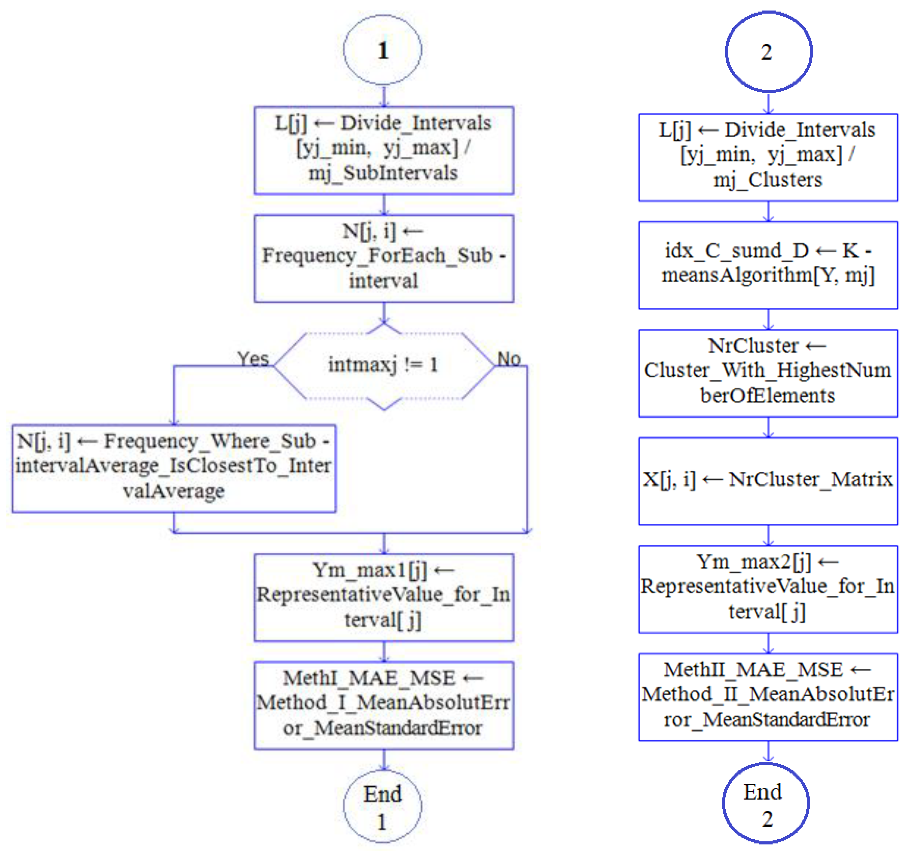
2.1. Method I
Suppose that the data series registered at k sites in n consecutive periods are given and let us denote by (yji) (j = 1, …, n) the series registered at the station i (i = 1, …, k).
Method I has the following stages [22].
- (I1)
- Establish the working intervals: compute the minimum (yj min) and maximum values (yj max), recorded at the jth moment (j = 1, …, n) and their amplitudes (Aj).
- (I2)
- Divide each interval [yj min, yj max] into mj subintervals with the length Lj = Aj/mj, (j = 1, …, n). The number of intervals is selected by the user, based on the user’s experience or different objective criteria.Each sub-interval should contain a sufficient number of values.
- (I3)
- Denote by Yjl, the subinterval l at the moment j and define its frequency, fjl, to be the number of values in Yjl, l = 1, …, mj, j = 1, …, n. Choose the interval whose frequency is maximum, denote it by Ij max and its frequency by fj max.
If there is more than one subinterval whose frequency is equal to fj max, then Ij max will be chosen to be that one whose average is closest to the average of the entire interval [yj min, yj max] (j = 1, …, n).
- (I4)
- Choose the average of the values in Ij max to be the representative value for the period j (j = 1, …, n).
- (I5)
- Compute the Mean Absolute Error (MAE) and Mean Standard Error (MSE) corresponding to all the observation sites.
- (I6)
- Represent graphically the results.
In the initial version of the algorithm, at stage (I3), the existence of at least two intervals with the same maximum frequencies and the same averages was not considered. Therefore, the initial algorithm might choose any of these intervals to be Ij max. Thus, many combinations may appear. To avoid this issue, at stage (I5), the average of all the values in the intervals with the equal maximum frequency will be the representative value for the period j. The implementation of the algorithm takes into account this situation.
2.2. Method II
Keeping the same notations as in Method I, Method II has the following stages [23].
- (II1)
- Choose the number of clusters, k and perform the k-means clustering to group the data series into clusters. This step returns an n-by-1 vector (idx) containing the cluster index for each observation site, the locations of the clusters’ centroids, within-cluster sums of point-to-centroid distances and distances from the points to the centroids.
- (II2)
- Determine the cluster containing the highest number of elements and build a matrix using the data series recorded at the sites from that cluster.
- (II3)
- Choose the value representing the period j as the average of the values recorded at j at the stations from the cluster with the highest number of observations.
- (II4)
- Compute the Mean Absolute Error (MAE) and Mean Standard Error (MSE) corresponding to all the observation sites.
- (II5)
- Represent the results graphically.
In this version of the algorithm, the number of clusters was chosen using the silhouette method, and the cluster selection has been made based on maximizing the ratio BSS/TSS×100, where BSS is the between sum of squares and TSS is the total sum of squares computed in the k-means algorithm [30,31,32]. If two or more clusters have the same number of elements (the highest one), the representative value computed at (II3) is the average of all the elements belonging to the cluster with the highest ratio.
2.3. Comparison of the Results
The model quality evaluation uses MSE, MAE and MAPE (mean absolute percentage error) computed for each series, and the average MSE, MAE and MAPE. The smaller the values of the indicators are, the better the estimation is. At least two indicators should be utilized for comparing the results (for cross-validation). Graphical representations of the fitted data and errors are also recommended.
2.4. Implementation
Climate Analyser was initially designed to implement the Most Probable Precipitation Method (Method I). In its actual form, it implements the methods described in Section 2.1 and Section 2.2. Based on the input data, it computes the maxima, minima and amplitude series, and to provide their graphical representation. Temperature and pollution trends over a region can also be modeled by utilizing this software.
After performing the spatial interpolation, the fitted series are displayed, together with the MAE and MSE series. If two methods have been performed, comparisons of the results are provided on the same chart. The computed MAE and MSE are exported in xls files for further analysis.
The work is in progress to implement the Thiessen Polygons Method and IDW interpolation and to provide comparisons between these methods. Another module will provide the frequency analysis for daily precipitation and temperature series, and the computation of the WMO indicators [28,29].
Data series are introduced in a Table (each series in a column) in a .csv file. The user can upload the file by clicking on the Select button and must provide the number of sub-intervals or clusters for running the algorithm. The methods that will be run may also be selected—the first one, the second one or both. After making this selection, one should click on Start button to perform the analysis.
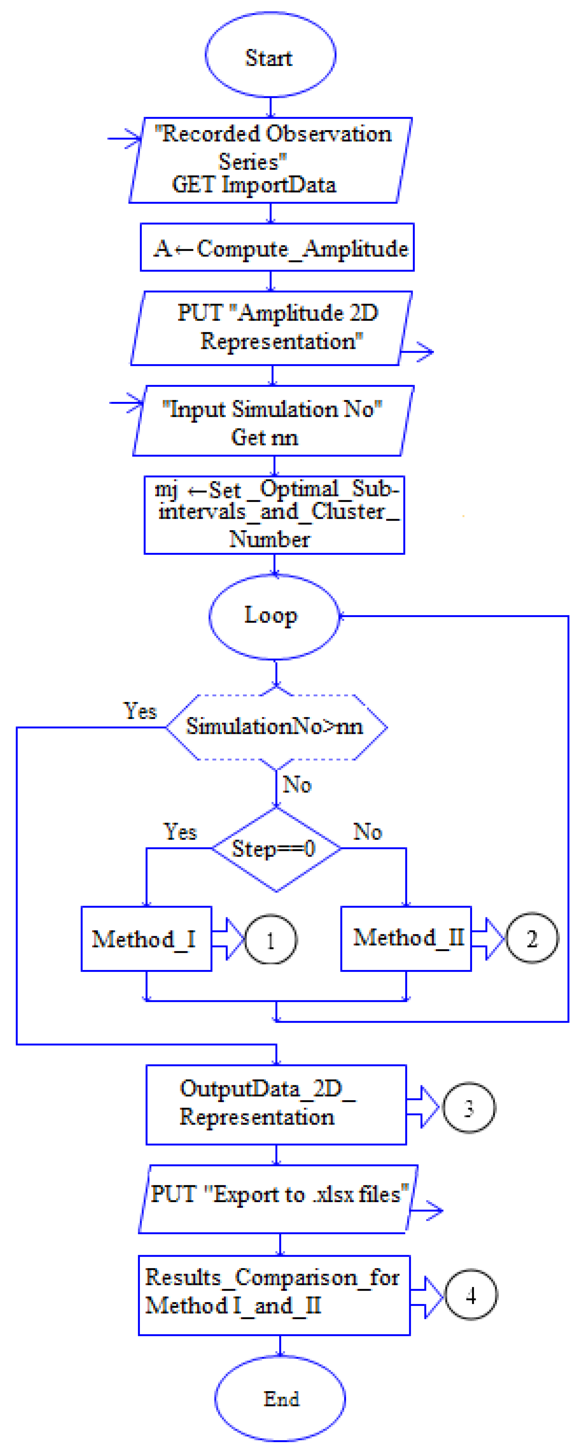
Figure 1 presents the interface of the software. The results are displayed in the six windows (Figure 1). The flowchart of the algorithm is shown in Figure 2.
The algorithm has the following steps:
- Compute_Amplitude step involves:
- -
- the calculation of the extreme values (yj min, respectively, yj max) for each j;
- -
- the amplitude computation for each j;
- Amplitude Representation step: amplitude 2D Graphical Representation.
- Choosing the number of subintervals or clusters.
Performing the modeling using Method I and Method II. Figure 3 shows the methods flowcharts.
- 4.
- Collecting the results in the Data Processing from Matlab destination tables.
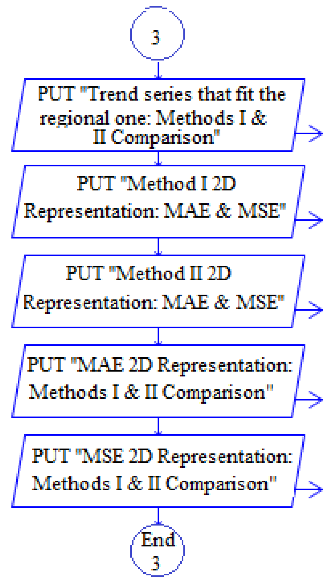
- 5.
- 2D graphical representations of “Trend series that fit the regional one”, MAE and MSE using both methods (presented in the next section) (Figure 4).
- 6.
- Export to file: the modeling output is exported to the xlsx files.
- 7.
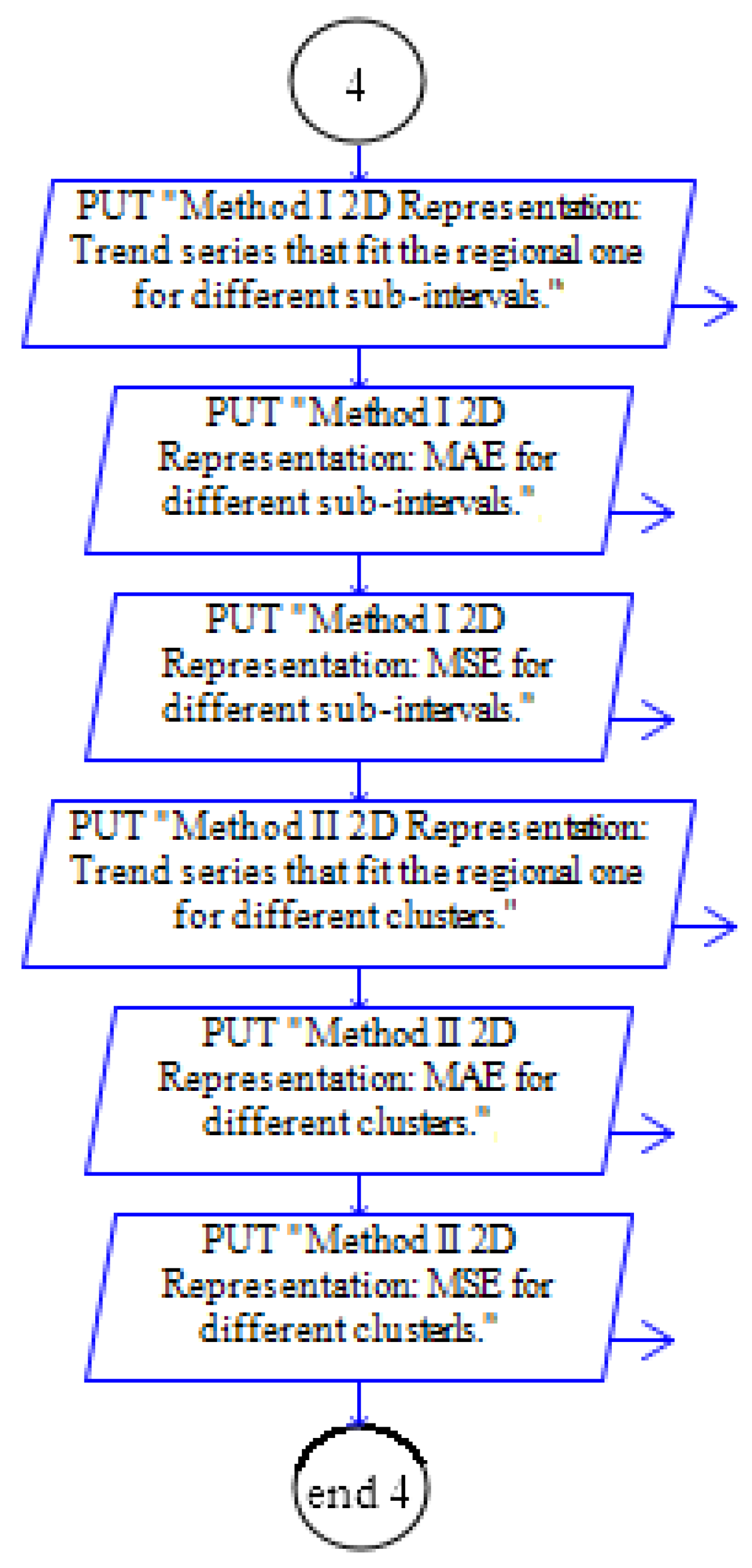
- Performing a comparative study, using both methods for different numbers of subintervals, respectively, different numbers of clusters and the graphical representation of the results for “Trend series that fit the regional one”, MAE and MSE (Figure 5).
2.5. Data Series
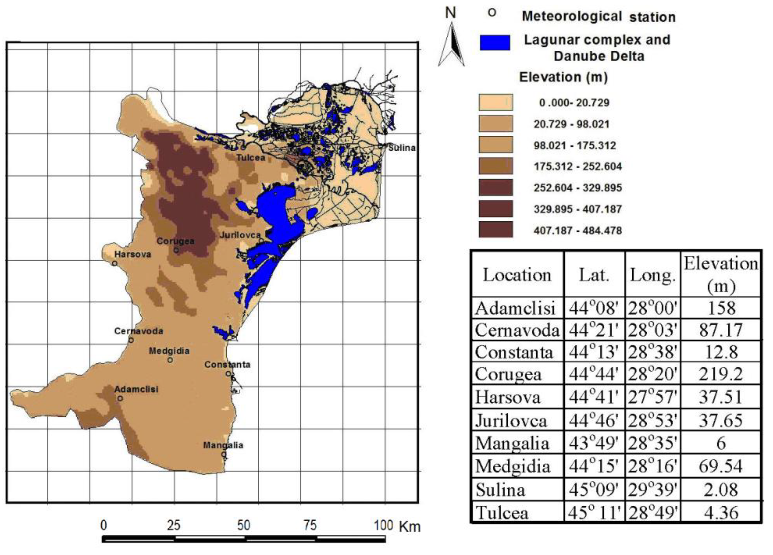
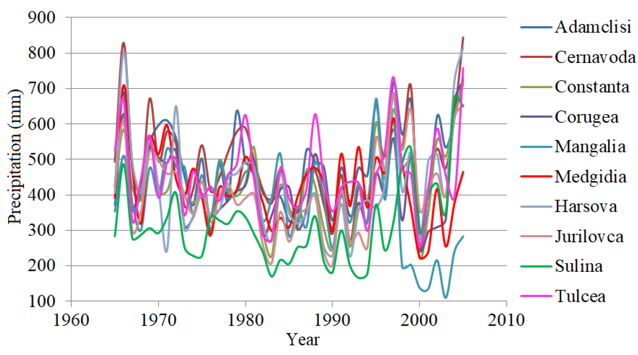
Data used for modeling consist of the annual precipitation series (recorded during 41 years at 10 meteorological stations situated in the southeastern part of Romania, in the Dobrogea region, between the Danube and the Black Sea (Figure 6).
Most of Dobrogea has an arid climate, with a mean annual temperature of about 10–11 °C and a summer mean annual temperature of 22–23 °C. The number of days with temperatures higher than 25 °C varies between 72 in Constanta and 95 in Tulcea. The average relative humidity varies between 78% and 85%, the lowest humidity being registered in the central and southern parts of the region. The mean annual precipitation is 350–450 mm. In the zone with the highest altitude, the mean annual precipitation values increase to about 450 mm. The 400 mm isohyet, parallel to the Black Sea Shore, delimitates the coastal region from the continental Dobrogea. Years with mean annual precipitation under 250 mm have been recorded as well [33]. The study series are represented in Figure 7. Among them, Sulina is situated 12 km offshore in the Danube Delta.
For this dataset, the ANOVA was performed in previous studies [22,25] to test if there is a difference between the series, followed by the Scheffe posthoc test. This test found that the Sulina series forms a separate group.
In [25,28,29], climate change in the area has been studied utilizing the daily data and the indices recommended by WMO. To give an idea about the precipitation occurrences, Table 1 contains the statistical distributions that best fit the annual precipitation series.
Readers may find information about the monthly and seasonal series trend in [29] and Dobrogea and its climate in [33,34,35]. Therefore, to exemplify how the software works, the annual data was chosen. All the mentioned results and related works, together with the present article, give a global picture of the precipitation dynamics in the Dobrogea region.
3. Results and Discussion
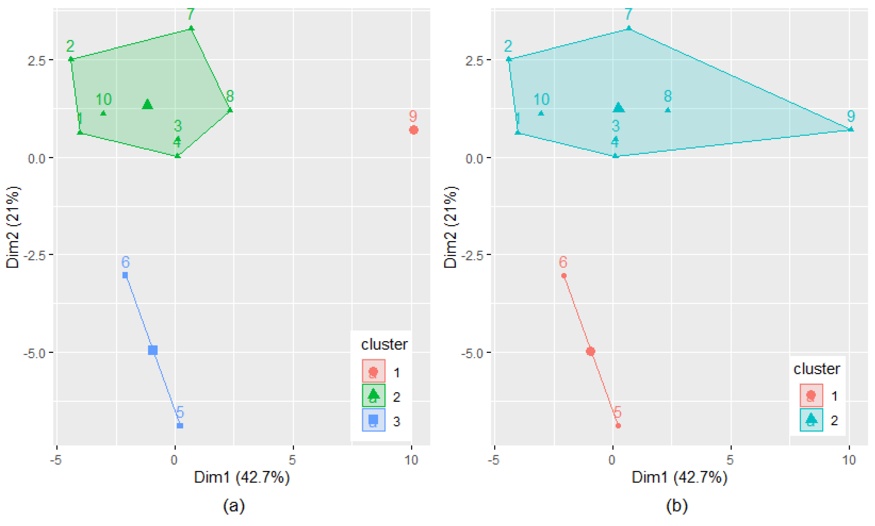
The optimal number of clusters has been determined to be three by the silhouette method and two by the elbow method. For comparison reasons, we present the results obtained when Method I was run with the number of intervals equal to the number of clusters—two and three. When using three clusters, the cluster with the highest number of elements contains all but Mangalia, Medgidia and Sulina (nos. 5, 6 and 9 in Table 1) series (Figure 8a). When using two clusters, the cluster with the highest number of elements contains all but Mangalia and Medgidia series (nos. 5 and 6, in Table 1) (Figure 8b). The clustering quality can be observed in Figure 8.
Based on the presented algorithm, the series Mangalia, Medgidia and Sulina or only the first two do not participate in the computation of the regional trend (when using three or two clusters). Therefore, the regional series is determined using the group containing homogenous data series (the cluster with the highest number of elements).
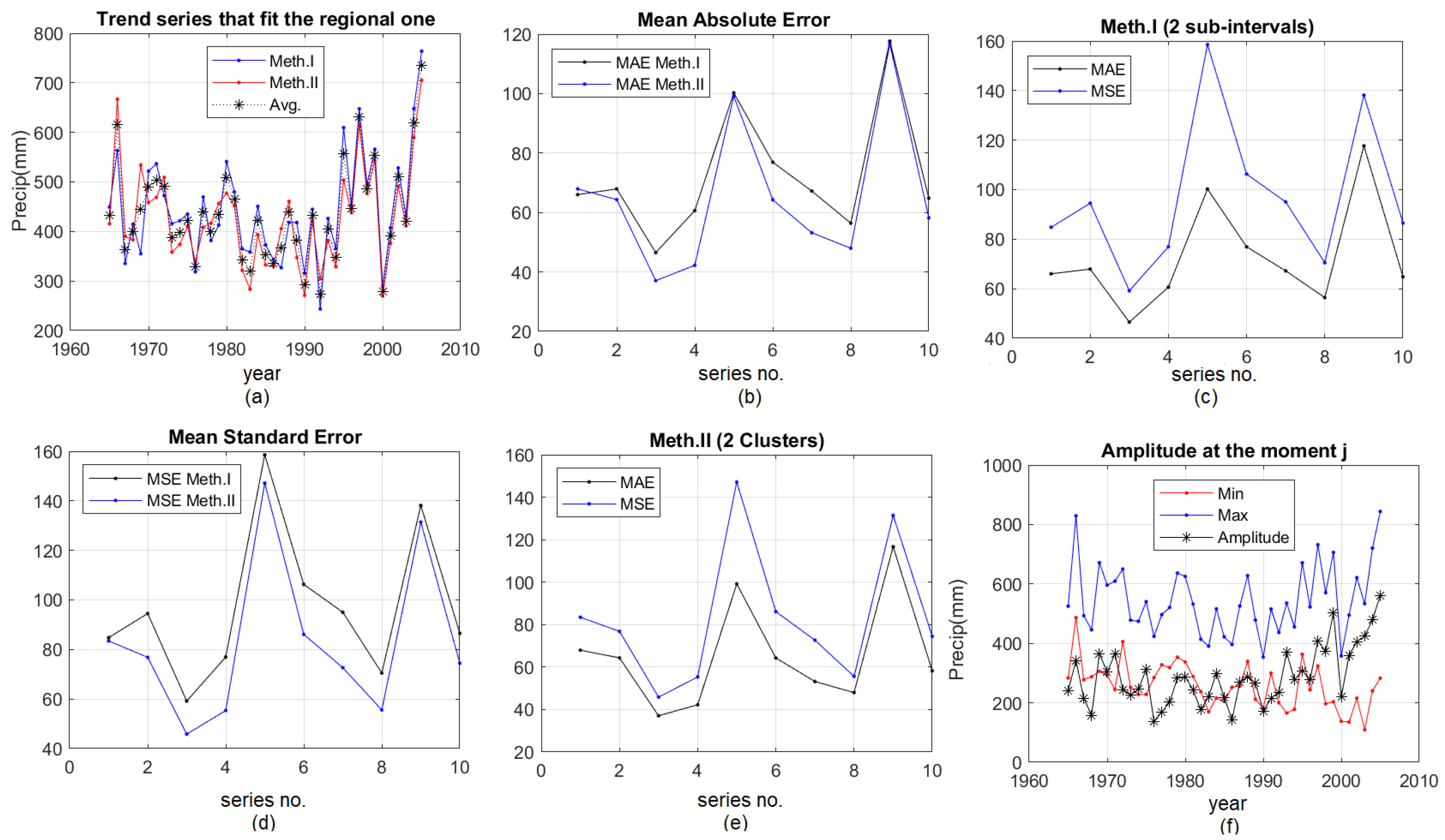
Figure 9 and Figure 10 presents the graphical results of fitting the regional trend of annual precipitation (“Trend series that fit the regional one”), the resulted mean absolute errors (MAE), the mean, standard errors (MSE) and Amplitude, when working with two (three) sub-intervals/clusters, using both methods.
The numbers from 1 to 10 represent the series as they are ordered in Table 1
In Figure 9a and Figure 10a, Meth. I and Meth. II refer to the results obtained using the first or the second method, and Avg. is the average series computed for each year by averaging the annual recorded values of all the 10 series. In Figure 9f and Figure 10f, Min and Max are the minimum and maximum precipitation series, respectively, and Amplitude is the difference between Max and Min series.
Notice the similar shapes of MAEs and MSEs in Figure 9c,e and Figure 10c,e, showing a similar pattern of the residual series. In most cases, MAEs and MSEs from Method I are higher than those from Method II (Figure 9b,d and Figure 10b,d).
Table 2 and Table 3 displays the MAE, MSE and MAPE computed using Method I (Method II). MAPE was utilized as extra goodness of fit indicator because it is non-dimensional, so it is recommended to compare different types of models [8].
MAPEs resulted from Method II are, in most cases, smaller than those from Method I. The average goodness of fit indicators (MAE, MSE and MAPE) are the smallest when using two clusters.
In Method I, MSE and MAPE are the smallest when working with two intervals, whereas MAE is the smallest in the case of three intervals. In Method II, all indicators are the smallest in the case of two clusters.
Figure 11 shows the comparisons of MAEs and MSEs for two and three sub-intervals/clusters. It confirms the best quality of the models when utilizing Method II with two clusters.
Comparison of the best model (Method II, two clusters) with Inverse Distance Weighting (IDW) and kriging are provided in Table 4. The best variogram model for the kriging was the exponential one, with the optimized parameters nugget = 1, sill = 2 and range = 24 [24].
The average MAE = 65.10, corresponding to MPPM (Method II), is the lowest compared to the average MAEs corresponding to IDW and kriging (KG), 71.11 and 84.40, respectively. For six out of 10 stations, MAEs computed in Method II are lower than those corresponding to IDW and KG. MAEs in IDW (KG) are the lowest for three (one) stations. The lowest average MSE was computed in KG (82.00). It is not significantly higher than the average MSE in MPPM (Method II), 82.68. MSEs in MPPM (IDW and KG, respectively) are the lowest for six (two and two, respectively) series. The average MAPE is the lowest when running Method II.
From these comparisons, one may notice the superior performances of Method II.
4. Conclusions
In this article, two algorithms for modeling the regional trend of precipitation have been presented, together with their implementation in Climate Analyser. To exemplify the functioning of this toolbox, a complete set of annual precipitation data, recorded for 41 years at 10 meteorological stations has been utilized, and the modeling results have been discussed. The main contributions of this work are twofold.
- The optimizing of finding the regional series, in the following two directions:
- The selection (in the k-means algorithm) of the clusters whose elements participate in the construction of the regional series, based on maximizing the ratio BSS/TSS×100. In the previous algorithm version [22,23], when two clusters have the same number of elements (maximum), each could be selected to build the regional series. In this version, choosing the maximum BSS/TSS×100 ensures a higher distance between the clusters and a smaller one inside them. Thus, the homogeneity degree of the series in the clusters is higher, so the estimation of the regional series is better than in the previous version of Method II.
- The choice of the values that participate in building the regional series when at least two subintervals have the same maximum frequency and absolute value of the difference between the subinterval average and the series average.
Let consider that and are such intervals, with the same maximum frequency, , m is the average precipitation in a specific year, and are the averages of and and = . Given that the values in the intervals are in ascending order, this means that ( so . Therefore, selecting would underestimate the regional series (since only the smallest values would participate in the evaluation of the regional series), while selecting would overestimate it; so the best choice is using the values in both intervals for building the regional series. - The second one is implementing the algorithm in user-friendly software, Climate Analyzer, freely available on request. It facilitates the computation of the regional trend. It also provides the graphical visualization of the output of the selected algorithm, offering the facility to compare the results for different segmentations of the series.
In the future, we intend to extend the software in the following directions:
- Implementing algorithms for determining the optimal number of clusters, given that the fitting quality depends on the number of groups involved in the regional series computation.
- implementing the IDW and Thiessen Polygons Methods.
- Extending the algorithm for analyzing the occurrence of precipitation events.
Author Contributions
Conceptualization, A.B.; methodology, A.B.; software, F.P.; validation, A.B., F.P. and C.Ș.D.; formal analysis, C.Ș.D.; investigation, A.B., F.P. and C.Ș.D.; resources, F.P.; data curation, A.B.; writing—original draft preparation, A.B., F.P. and C.Ș.D.; writing—review and editing, A.B.; visualization, F.P.; supervision, A.B.; project administration, A.B.; funding acquisition, A.B. All authors have read and agreed to the published version of the manuscript.
Funding
This research received no external funding.
Institutional Review Board Statement
Not applicable.
Informed Consent Statement
Not applicable.
Data Availability Statement
Data series will be available on request.
Conflicts of Interest
The authors declare no conflict of interest.
References
- Report of the 21st Session on the CLIVAR Scientific Steering Group. In Proceedings of the 21st Session of the CLIVAR Scientific Steering Group, Moscow, Russia, 10–12 November 2014. ICPO Publication Series No. 201 WCRP Informal Report No. 3/2015.
- Schneider, T.; Teixeira, J.; Bretherton, C.S.; Brient, F.; Pressel, K.G.; Schär, C.; Siebesma, A.P. Climate goals and computing the future of clouds. Nat. Clim. Chang. 2017, 7, 3–5. [Google Scholar] [CrossRef]
- Hiez, G. Homogénéisation des données pluviométriques. Cah. ORSTOM Hydrol. 1997, XIX, 129–172. [Google Scholar]
- El Alaoui El Fels, A.; El Mehdi Saidi, M.; Bouiji, A.; Benrhanem, M. Rainfall regionalization and variability of extreme precipitation using artificial neural networks: A case study from western central Morocco. J. Water Clim. Chang. 2021, 12, 1107–1122. [Google Scholar] [CrossRef] [Green Version]
- Srinivas, V.V. Regionalization of Precipitation in India—A Review. J. Indian Inst. Sci. 2013, 93, 153–162. [Google Scholar]
- Li, J.; Heap, A.D. Spatial interpolation methods applied in the environmental sciences: A review. Environ. Model. Softw. 2014, 53, 173–189. [Google Scholar] [CrossRef]
- Bărbulescu, A.; Șerban, C.; Indrecan, M.-L. Improving spatial interpolation quality. IDW versus a genetic algorithm. Water 2021, 13, 863. [Google Scholar] [CrossRef]
- Bărbulescu, A.; Băutu, A.; Băutu, E. Particle Swarm Optimization for the Inverse Distance Weighting Distance method. Appl. Sci. 2020, 10, 2054. [Google Scholar] [CrossRef] [Green Version]
- Ly, S.; Charles, C.; Degré, C. Different methods for spatial interpolation of rainfall data for operational hydrology and hydrological modeling at watershed scale: A review. Biotechnol. Agron. Soc. Environ. 2013, 17, 392–406. [Google Scholar]
- Wu, K.-Y.; Mossa, J.; Mao, L.; Almulla, M. Comparison of different spatial interpolation methods for historical hydrographic data of the lowermost Mississippi River. Ann. GIS 2019, 2, 133–151. [Google Scholar] [CrossRef]
- Lloyd, C. Assessing the effect of integrating elevation data into the estimation of monthly precipitation in Great Britain. J. Hydrol. 2005, 308, 128–150. [Google Scholar] [CrossRef]
- Kurtzman, D.; Navon, S.S.; Morin, E. Improving interpolation of daily precipitation for hydrologic modelling: Spatial patterns of preferred interpolators. Hydrol. Process. 2009, 23, 3281–3291. [Google Scholar] [CrossRef]
- Zhang, X.; Srinivasan, R. GIS-Based spatial precipitation estimation: A comparison of geostatistical approaches. J. Am. Water Resour. Assoc. 2009, 45, 894–906. [Google Scholar] [CrossRef]
- Liu, H.; Chen, S.; Hou, M.; He, L. Improved inverse distance weighting method application considering spatial autocorrelation in 3D geological modeling. Earth Sci. Inform. 2020, 13, 619–632. [Google Scholar] [CrossRef]
- Liu, Z.; Zhang, Z.; Zhou, C.; Ming, W.; Du, Z. An Adaptive Inverse-Distance Weighting Interpolation Method Considering Spatial Differentiation in 3D Geological Modeling. Geosciences 2021, 11, 51. [Google Scholar] [CrossRef]
- Ozelkan, E.; Bagis, S.; Ozelkan, E.C.; Ustundag, B.B.; Yucel, M.; Ormeci, C. Spatial interpolation of climatic variables using land surface temperature and modified inverse distance weighting. Int. J. Remote Sens. 2015, 36, 1000–1025. [Google Scholar] [CrossRef]
- Jiang, W.; Zhang, P.; Jiang, H.; Zhao, X. Reconstructing Satellite-Based Monthly Precipitation over Northeast China Using Machine Learning Algorithms. Remote Sens. 2017, 9, 781. [Google Scholar] [CrossRef] [Green Version]
- Ryu, S.; Song, J.J.; Kim, Y.; Sung-Hwa, J.; Younghae, D.; GyuWon, L. Spatial Interpolation of Gauge Measured Rainfall Using. Asia-Pac. J. Atmos. Sci. 2021, 57, 331–345. [Google Scholar] [CrossRef] [Green Version]
- Dragomir, F.L. Theoretical Bases of the Process Simulation; Sitech: Craiova, Romania, 2017. [Google Scholar]
- Dragomir, F.L. Modeling and Simulating the Systems and Processes; Editura Universității Naționale de Apărare Carol I: București, Romania, 2017. [Google Scholar]
- Dragomir, F.L. Decision Theory—Theoretical Notions; Editura Universității Naționale de Apărare Carol I: București, Romania, 2017. [Google Scholar]
- Bărbulescu, A. A new method for estimation the regional precipitation. Water Resour. Manag. 2016, 30, 33–42. [Google Scholar] [CrossRef]
- Bărbulescu, A.; Nazzal, Y.; Howari, F. Statistical analysis and estimation of the regional trend of aerosol size over the Arabian Gulf Region during 2002–2016. Sci. Rep. 2018, 8, 9571. [Google Scholar] [CrossRef] [Green Version]
- Bărbulescu, A.; Barbes, L.; Nazzal, Y. New model for inorganic pollutants dissipation on the northern part of the Romanian Black Sea coast. Rom. J. Phys. 2018, 63, 806. [Google Scholar]
- Bărbulescu, A. Studies on Time Series. Applications in Environmental Sciences; Springer: Cham, Switzerland, 2016. [Google Scholar]
- Zhang, Q.; Han, J.; Yang, Z. Spatiotemporal characteristics of regional precipitation events in the Jing-Jin-Ji region during 1989–2018. Int. J. Climatol. 2002, 41, 1190–1198. [Google Scholar] [CrossRef]
- Chiles, J.-P.; Delfiner, P. Geostatistics. Modeling Spatial Uncertainty, 2nd ed.; Wiley: Hoboken, NJ, USA, 2002. [Google Scholar]
- Bărbulescu, A.; Deguenon, J. Change point detection and models for precipitation evolution. Case study. Rom. J. Phys. 2014, 59, 590–600. [Google Scholar]
- Deguenon, J.; Bărbulescu, A. Trends of extreme precipitation events in Dobrudja. Ovidius Univ. Ann. Ser. Civil Eng. 2011, 1, 73–80. [Google Scholar]
- Soetewey, A.; Stats, R. Available online: https://statsandr.com/blog/clustering-analysis-k-means-and-hierarchical-clustering-by-hand-and-in-r/ (accessed on 20 May 2021).
- Al-Taani, A.; Nazzal, Y.; Howari, F.; Iqbal, J.; Bou-Orm, N.; Xavier, C.M.; Bărbulescu, A.; Sharma, M.; Dumitriu, C.Ș. Contamination assessment of heavy metals in soil, Liwa area, UAE. Toxics 2021, 9, 53. [Google Scholar] [CrossRef] [PubMed]
- Nazzal, Y.H.; Bărbulescu, A.; Howari, F.; Al-Taani, A.A.; Iqbal, J.; Xavier, C.M.; Sharma, M.; Dumitriu, C.Ș. Assessment of metals concentrations in soils of Abu Dhabi Emirate using pollution indices and multivariate statistics. Toxics 2021, 9, 95. [Google Scholar] [CrossRef] [PubMed]
- Bărbulescu, A.; Maftei, C.; Bautu, E. Modeling the Hydro-Meteorological Time Series. Applications to Dobrudja Region; Lambert Academic Publishing: Saarbrucken, Germany, 2010. [Google Scholar]
- Bărbulescu, A.; Maftei, C. Statistical approach of the behavior of Hamcearca River (Romania). Rom. Rep. Phys. 2021, 73, 703. [Google Scholar]
- Bărbulescu, A.; Maftei, C.; Dumitriu, C.S. The modeling of the climatic process that participates at the sizing of an irrigation system. Bull. Appl. Comput. Math 2002, CII-2048, 11–20. [Google Scholar]
Figure 1.
The interface.

Figure 2.
The algorithm flowchart.

Figure 3.
Logical scheme for Method I (the left-hand side) and Method II (the right-hand side).

Figure 4.
Output.

Figure 5.
Comparison step.

Figure 6.
Dobrogea region and the meteorological stations.

Figure 7.
The annual precipitation series.

Figure 8.
Clustering the data series: (a) three and (b) two clusters.

Figure 9.
Study results when using two intervals/clusters (a) “Trend series that fit the regional one”; (b) MAE in both methods; (c) MAE and MSE in Method I; (d) MSEs from both methods; (e) MAE and MSE from Method II; (f) Minimum, Maximum and Amplitude Series amplitude.
Figure 9.
Study results when using two intervals/clusters (a) “Trend series that fit the regional one”; (b) MAE in both methods; (c) MAE and MSE in Method I; (d) MSEs from both methods; (e) MAE and MSE from Method II; (f) Minimum, Maximum and Amplitude Series amplitude.

Figure 10.
Study results when using three intervals/clusters (a) “Trend series that fit the regional one”; (b) MAE in both methods; (c) MAE and MSE in Method I; (d) MSEs from both methods; (e) MAE and MSE from Method II; (f) Minimum, Maximum and Amplitude Series amplitude.
Figure 10.
Study results when using three intervals/clusters (a) “Trend series that fit the regional one”; (b) MAE in both methods; (c) MAE and MSE in Method I; (d) MSEs from both methods; (e) MAE and MSE from Method II; (f) Minimum, Maximum and Amplitude Series amplitude.

Figure 11.
Comparative results when using three intervals/clusters (a) “Trend series that fit the regional one” in Method I; (b) MAE in Method I; (c) MSE in Method I; (d) “Trend series that fit the regional one” in Method II; (e) MAE in Method II; (f) MSE in Method II.
Figure 11.
Comparative results when using three intervals/clusters (a) “Trend series that fit the regional one” in Method I; (b) MAE in Method I; (c) MSE in Method I; (d) “Trend series that fit the regional one” in Method II; (e) MAE in Method II; (f) MSE in Method II.


Table 1.
The statistical distributions that best fit the annual precipitation series.
| Crt. No | Series | Distribution | Parameters | Kolmogorov- Smirnov | Chi- Squared | Reject the Null |
|---|---|---|---|---|---|---|
| 1 | Adamclisi | Wakeby | α = 185.8 β = 4.148 γ = 249.34 δ = −0.55834 ξ = 288.45 | 0.9631 | 0.94298 | No |
| 2 | Cernavoda | Log-logistic (3P) | A = 7.853 β = 530.76 γ = −56.791 | 0.9987 | 0.78226 | No |
| 3 | Constanta | Wakeby | α = 1396.7 β = 8.6357 γ = 131.68 δ = −0.17477 ξ = 169.03 | 0.9793 | 0.98812 | No |
| 4 | Corugea | GEV | k = 0.07952 σ = 80.002 μ = 363.68 | 0.9663 | 0.9776 | No |
| 5 | Mangalia | Johnson SB | γ = −1.5528 δ = 5.7129 λ = 2959.6 ξ = −1305.7 | 0.9972 | 0.9711 | No |
| 6 | Medgidia | Log-logistic (3P) | α = 19.78 β = 1142.3 γ = −723.44 | 0.9987 | 0.9284 | No |
| 7 | Harsova | Pearson 6 (4P) | α 1 = 38.828 α2 = 10.541 β = 93.195 γ = 47.668 | 0.9555 | 0.9835 | No |
| 8 | Jurilovca | Generalized logistic | k = 0.10343 σ = 68.053 μ = 397.14 | 0.9946 | 0.9666 | No |
| 9 | Sulina | Wakeby | α = 395.83 β = 4.3011 γ = 80.116 δ = 0.14853 ξ = 148.9 | 0.9975 | 0.9908 | No |
| 10 | Tulcea | Burr | k = 0.94537 α = 7.5822 β = 436.52 | 0.9820 | 0.9281 | No |
Table 2.
The goodness of fit indicators in Methods I with two and three intervals for annual precipitation.
Table 2.
The goodness of fit indicators in Methods I with two and three intervals for annual precipitation.
| MAE | MSE | MAPE | |||||
|---|---|---|---|---|---|---|---|
| Crt. No | Station | 2 | 3 | 2 | 3 | 2 | 3 |
| 1 | Adamclisi | 66.01 | 69.46 | 84.80 | 92.00 | 13.03 | 14.10 |
| 2 | Cernavoda | 67.92 | 63.84 | 94.52 | 83.04 | 13.07 | 12.36 |
| 3 | Constanta | 46.50 | 47.72 | 59.16 | 64.98 | 11.75 | 12.20 |
| 4 | Corugea | 60.62 | 50.77 | 76.95 | 73.44 | 15.47 | 13.42 |
| 5 | Mangalia | 100.24 | 107.67 | 158.57 | 164.93 | 43.58 | 45.32 |
| 6 | Medgidia | 76.91 | 73.71 | 106.27 | 101.39 | 19.47 | 19.50 |
| 7 | Harsova | 67.21 | 55.60 | 95.03 | 82.00 | 17.36 | 15.33 |
| 8 | Jurilovca | 56.41 | 64.30 | 70.49 | 83.69 | 15.91 | 18.75 |
| 9 | Sulina | 117.66 | 126.95 | 138.15 | 149.82 | 45.35 | 48.47 |
| 10 | Tulcea | 64.81 | 56.26 | 86.52 | 78.52 | 14.15 | 12.88 |
| Average | 72.43 | 71.63 | 97.04 | 97.38 | 20.91 | 21.23 | |
Table 3.
The goodness of fit indicators in Methods II with two and three clusters for annual precipitation.
Table 3.
The goodness of fit indicators in Methods II with two and three clusters for annual precipitation.
| Crt. No | MAE | MSE | MAPE | ||||
|---|---|---|---|---|---|---|---|
| Station | 2 | 3 | 2 | 3 | 2 | 3 | |
| 1 | Adamclisi | 67.93 | 61.42 | 83.45 | 74.52 | 13.55 | 12.42 |
| 2 | Cernavoda | 64.34 | 53.38 | 76.82 | 66.85 | 12.58 | 10.26 |
| 3 | Constanta | 37.07 | 40.70 | 45.83 | 48.44 | 9.15 | 10.38 |
| 4 | Corugea | 42.23 | 45.41 | 55.35 | 58.81 | 11.17 | 12.11 |
| 5 | Mangalia | 99.15 | 102.46 | 146.16 | 148.51 | 41.16 | 42.24 |
| 6 | Medgidia | 64.27 | 60.78 | 86.10 | 83.22 | 16.61 | 15.94 |
| 7 | Harsova | 53.18 | 55.93 | 72.65 | 75.63 | 13.40 | 14.75 |
| 8 | Jurilovca | 47.98 | 54.62 | 55.60 | 64.18 | 13.62 | 15.85 |
| 9 | Sulina | 116.69 | 131.28 | 130.43 | 147.86 | 43.62 | 49.07 |
| 10 | Tulcea | 58.21 | 58.21 | 74.47 | 67.90 | 12.70 | 12.25 |
| Average | 65.10 | 66.06 | 82.68 | 83.59 | 18.76 | 19.52 | |
Table 4.
Comparison of the performances of Method II, IDW and kriging.
| MPPM (Method II) | IDW | Kriging | |||||||
|---|---|---|---|---|---|---|---|---|---|
| MAE | MSE | MAPE | MAE | MSE | MAPE | MAE | MSE | MAPE | |
| Adamclisi | 67.93 | 83.45 | 13.55 | 60.08 | 70.22 | 12.41 | 82.03 | 68.85 | 12.08 |
| Cernavoda | 64.34 | 76.82 | 12.58 | 53.81 | 71.00 | 10.25 | 65.23 | 81.15 | 14.12 |
| Constanta | 37.07 | 45.83 | 9.15 | 48.17 | 59.90 | 12.78 | 43.22 | 51.35 | 11.39 |
| Corugea | 42.23 | 55.35 | 11.17 | 49.23 | 62.40 | 10.93 | 46.04 | 61.65 | 10.32 |
| Mangalia | 99.15 | 146.16 | 41.16 | 56.91 | 72.64 | 13.67 | 56.34 | 70.75 | 13.54 |
| Medgidia | 64.27 | 86.10 | 16.61 | 47.20 | 57.11 | 11.44 | 50.19 | 61.64 | 14.63 |
| Harsova | 53.18 | 72.65 | 13.40 | 61.71 | 84.26 | 54.81 | 62.21 | 84.26 | 54.75 |
| Jurilovca | 47.98 | 55.60 | 13.62 | 69.90 | 88.14 | 25.83 | 61.24 | 75.83 | 20.42 |
| Sulina | 116.69 | 130.43 | 43.62 | 171.23 | 182.93 | 74.79 | 261.63 | 170.87 | 58.74 |
| Tulcea | 58.21 | 74.47 | 12.70 | 92.90 | 111.51 | 14.75 | 75.92 | 93.65 | 13.21 |
| Average | 65.10 | 82.68 | 18.76 | 71.11 | 84.29 | 24.17 | 84.40 | 82.00 | 22.32 |
Publisher’s Note: MDPI stays neutral with regard to jurisdictional claims in published maps and institutional affiliations. |
© 2021 by the authors. Licensee MDPI, Basel, Switzerland. This article is an open access article distributed under the terms and conditions of the Creative Commons Attribution (CC BY) license (https://creativecommons.org/licenses/by/4.0/).
Share and Cite
MDPI and ACS Style
Bărbulescu, A.; Postolache, F.; Dumitriu, C.Ș. Estimating the Precipitation Amount at Regional Scale Using a New Tool, Climate Analyzer. Hydrology 2021, 8, 125. https://0-doi-org.brum.beds.ac.uk/10.3390/hydrology8030125
AMA Style
Bărbulescu A, Postolache F, Dumitriu CȘ. Estimating the Precipitation Amount at Regional Scale Using a New Tool, Climate Analyzer. Hydrology. 2021; 8(3):125. https://0-doi-org.brum.beds.ac.uk/10.3390/hydrology8030125
Chicago/Turabian StyleBărbulescu, Alina, Florin Postolache, and Cristian Ștefan Dumitriu. 2021. "Estimating the Precipitation Amount at Regional Scale Using a New Tool, Climate Analyzer" Hydrology 8, no. 3: 125. https://0-doi-org.brum.beds.ac.uk/10.3390/hydrology8030125
Note that from the first issue of 2016, this journal uses article numbers instead of page numbers. See further details here.