Article

Impact of Climate Change on the Hydrology of the Upper Awash River Basin, Ethiopia

1
College of Forestry and Natural Resources, Hawassa University, Shashemene P.O. Box 128, Ethiopia
2
CGIAR Research Program on Climate Change, Agriculture and Food Security (CCAFS), International Livestock Research Institute (ILRI), P.O. Box 30709, Nairobi 00100, Kenya
3
Wetland Research Unit, UCL Department of Geography, University College London, Gower Street, London WC1E 6BT, UK
4
World Agroforestry (ICRAF), United Nations Avenue, P.O. Box 30677, Nairobi 00100, Kenya
5
Department of Agronomy, University of Fort Hare, 1 King Williamstown Rd, Alice 5700, South Africa
6
Stockholm Environment Institute—Africa, World Agroforestry, P.O. Box 30677, Nairobi 00100, Kenya
7
International Livestock Research Institute, Naivasha Road, P.O. Box 30677, Nairobi 00100, Kenya
*
Author to whom correspondence should be addressed.
Submission received: 12 November 2021 / Revised: 18 December 2021 / Accepted: 20 December 2021 / Published: 23 December 2021
(This article belongs to the Section Hydrology–Climate Interactions)

Abstract

:
This study investigated the impacts of climate change on the hydrology of the Upper Awash Basin, Ethiopia. A soil and water assessment tool (SWAT) model was calibrated and validated against observed streamflow using SWAT CUP. The Mann–Kendall trend test (MK) was used to assess climate trends. Meteorological drought (SPEI) and hydrological drought (SDI) were also investigated. Based on the ensemble mean of five global climate models (GCMs), projected increases in mean annual maximum temperature over the period 2015–2100 (compared with a 1983–2014 baseline) range from 1.16 to 1.73 °C, while increases in minimum temperature range between 0.79 and 2.53 °C. Increases in mean annual precipitation range from 1.8% at Addis Ababa to 45.5% over the Hombole area. High streamflow (Q5) declines at all stations except Ginchi. Low flows (Q90) also decline with Q90 equaling 0 m3 s−1 (i.e., 100% reduction) at some gauging stations (Akaki and Hombole) for individual GCMs. The SPEI confirmed a significant drought trend in the past, while the frequency and severity of drought will increase in the future. The basin experienced conditions that varied from modest dry periods to a very severe hydrological drought between 1986 and 2005. The projected SDI ranges from modestly dry to modestly wet conditions. Climate change in the basin would enhance seasonal variations in hydrological conditions. Both precipitation and streamflow will decline in the wet seasons and increase in the dry seasons. These changes are likely to have an impact on agricultural activities and other human demands for water resources throughout the basin and will require the implementation of appropriate mitigation measures.

1. Introduction

Scientific evidence is unequivocal that the earth’s climate is changing. Due to increasing atmospheric concentrations of greenhouse gases, the average surface temperature of the earth has increased by 1 °C with a likely range of 0.8 to 1.2 °C since the preindustrial period [1,2,3]. Projections from a wide range of climate model simulations suggest that the average global temperature will increase between 1.1 and 5.4 °C by 2100 [3,4]. Projections of increases in temperature over the African continent for the end of the 21st century are in the range of 1.5 °C under a low-emission scenario (RCP 2.6) to 5.0 °C under a high-emission scenario (RCP 8.5) [1,5,6,7,8].
Climate change will have significant impacts on the hydrological cycle [9,10], which will include alterations to precipitation and evapotranspiration [4]. For example, a study conducted using four Intergovernmental Panel on Climate Change (IPCC) emission scenarios (A1FI, A2, B1, and B2) and five GCMs (HadCM3, PCM, CGCM2, CSIRO2, and ECHAM4) (2000–2100) reported that annual precipitation over the Horn of Africa (including Ethiopia) could decrease by 25% [5]. Conversely, another study [11] suggested that while long-term annual precipitation for Ethiopia may increase by around 9%, the largest seasonal declines are projected for the driest quarter of the year (February–May), especially in those regions that are already relatively dry.
Previous studies have suggested that climate change will significantly affect hydrological systems and the water resources of Ethiopia [12,13,14,15,16]. For instance, a study in the Gilgel Abay catchment, the source of Blue Nile in northern Ethiopia, indicated that a modeled 2 °C temperature increase could lead to a decline in seasonal and annual runoff of around 33% and 20%, respectively [17]. A study in Ethiopia’s Meki River catchment also established that a 1.5 °C increase in temperature resulted in a 6% increase in potential evapotranspiration and a 13% decrease in streamflow [13]. Based on the IPCC Special Report on Emission Scenarios (SRES), the average annual inflow into Lake Ziway in the Rift Valley Basin might be reduced by 19% and 27% for the A2a (heterogeneous future world with regionally oriented economies) and B2a (regionally oriented but with a general evolution towards environmental protection and social equity) scenarios, respectively [16].
The Awash River Basin, which has a total area of 110,000 km2 and a human population of more than 10 million, is one of the most important basins in Ethiopia [18]. However, increasing desertification and declines in river flow are among the problems the basin and its inhabitants have experienced for the past three decades [18]. While the causes of desertification and flow reduction are usually attributed to climate change, establishing the influence of a changing climate on river flow reduction and the hydrology of the basin requires more detailed studies. Furthermore, potential future climate change impacts on hydrological conditions within the basin must be assessed to establish robust water resource planning and management. This will help policymakers in the development of appropriate water resource strategies that consider future climate change, and ensure sustainable utilization of water and associated resources.
Previous investigations of the impacts of climate change on the Awash River Basin have included hydrological modelling assessments employing earlier generation (SRES) emission scenarios as simulated by one GCM [19] and the application of one or more representative concentration pathway (RCP) scenarios provided by a number (two [20] three [21]) of climate models. Results of these studies included projected declines in annual rainfall of 9.9%, an increase in mean temperature of 0.9 °C, and a resultant decline in annual streamflow of 11.5% under RCP4.5 in the 2080s [20]. Increases in water deficiency in all seasons for parts of the basin were projected as a result of these increases in temperature and declines in precipitation [21]. A further study extended these investigations by considering not only the uncertainty associated with different emission (RCP) scenarios and GCMs but also an alternative hydrological model structure [22]. It demonstrated that while GCM-related uncertainty was dominant and was characterized by both increases and decreases in discharge, model structural uncertainty can be considerable, especially for low flows [22].
The current study further deepens knowledge of climate change impacts on the hydrology of the upstream part of the Awash Basin by investigating both the recent historical period (1983–2014) and the remainder of the current century (2015–2100). It includes trend analysis of observed hydrometeorological data, hydrological modelling, and the evaluation of meteorological and hydrological drought indices. The widely used hydrological model Soil and Water Assessment Tool (SWAT) developed by the US Department of Agriculture Research Service [23] is used to simulate the hydrology of the basin. The model is calibrated and validated using the SUFI2 algorithm in the SWAT CUP program [24]. Projections from five GCMs for the representative concentration pathway (RCP) 4.5 emission scenarios were selected based on data availability and coverage. These projections have been downscaled and bias-corrected [25] using historical climate data for the period 1983–2014. Uncertainties associated with GCMs and the downscaling techniques could result in significant differences in simulated hydrological conditions [26]. These uncertainties, particularly those related to inherent errors of the models, can be reduced by using a multimodel ensemble mean of the GCMs, and several studies have suggested using a multimodel ensemble to minimize the biases and uncertainties of future climate simulations [26,27,28]. Accordingly, this study uses both individual downscaled GCMs and the ensemble mean from all of the GCMs. The downscaled climate data were then used as input to the SWAT model to simulate impacts on river discharge. The novelty of the study lies in the combination of trend assessment for both past decades and future projections, evaluation of climate change impacts on hydrological extremes, and the implications for both meteorological and hydrological drought.

2. Materials and Methods

2.1. Study Area

The Upper Awash River Basin is located in the North West Rift Valley of Ethiopia and has an area of around 11,430 km2. The river rises on the high plateau near Ginchi town, west of Addis Ababa, at an altitude of more than 3000 m. The total length of the main course of the river is 336 km (Figure 1).
The climate of the basin varies from humid subtropical to semiarid. Based on data from meteorological stations for the period 1983 to 2014 obtained from the National Meteorological Agency of Ethiopia, the mean maximum annual temperature ranges from 23.3 to 28.0 °C, while the mean annual minimum temperature ranges from 9.5 to 13.3 °C. The basin receives most of its precipitation in two main seasons, spring and summer. Spring, which is locally named Bulg, is a short rainy season from March to May. Summer, known locally as Kiremt, is the main rain and crop-growing season and extends from June to September. Hombole and Tulu Bolo receive over 60% of their annual total rainfall in summer and 20% in spring. The other four stations receive more than 40% in summer and 30% in spring. The mean annual rainfall ranges from 600 mm at the Hombole meteorological station to 1094 mm at the Ginchi station.

2.2. Data and Methods

2.2.1. Downscaling Climate Variables and Simulation Performance

This study used downscaled outputs from five GCMs (Table 1) for the RCP4.5 emission scenario. This is an intermediate emission scenario of long-term global emissions of greenhouse gases, short-lived species, and land use/land cover, which stabilizes radiative forcing at 4.5 W m−2 in the year 2100 [29]. RCP4.5 represents generally good agreement with the latest policies for lower greenhouse gas emissions by the global community [30].
The GCMs provide projections of future climate at resolutions of hundreds of kilometers and must be resampled at a higher spatial resolution to be used in studies of the impact of change, including those that focus on hydrological impacts using catchment modelling [31]. Therefore, the GCM projections were downscaled using a statistical downscaling model (SDSM) to project future temperature and precipitation across the Upper Awash River Basin.
Before downscaling the climate variables for each station, the simulation performance of each GCM was assessed to validate their accuracy in representing observed climate. For this purpose, we used observed and historical GCM daily data for the period 1983–2005. The mean relative error (MRE) (Equation (1)) was used to define the model simulation error, the correlation coefficient (CORR) (Equation (2)) identified the similarity or otherwise of observed and simulated climate data, and the Nash–Sutcliffe efficiency coefficient (NSE) (Equation (3)) was further used to evaluate the GCMs’ capability in simulating climate variables. The smaller the value of the MRE is, the higher the GCM simulation capability is [32], while the closer the NSE value is to 1, the better is the model simulation performance [32].
M R E = P ¯ O ¯ O ¯ 100
C O R R = i = 1 N P i P ¯ O i O ¯ ( i = 1 N P i P ¯ 2 ) 0.5 ( ( i = 1 N O i O ¯ 2 ) 0.5
N S E = 1 ( i = 1 N P i O i 2 ( i = 1 N O i O ¯ 2
where Pi and Oi are the values at the ith time step (daily) in the downscaled GCM simulation and observational time series, respectively, P ¯ and O ¯ are the mean value of the downscaled GCM simulation and observational sequence, and N is the total sample number [32].
An SDSM is an established decision support tool for assessing local climate change impacts using a robust statistical downscaling technique (see [33] for a detailed review of its conceptual basis). It is computationally inexpensive and thus can be easily applied to outputs from multiple GCM experiments to provide specific local climate information [34]. The tool is designed to identify local or regional climate information by determining a statistical model that relates large-scale climate variables (the predictors) to regional or local variables (the predictand) [31].
An SDSM was used to define statistical models using daily observed data (i.e., local climate data for a specific location for the predictand and larger-scale National Centers for Environmental Prediction (NCEP) data for the predictors). These models are then used with GCM-derived predictors to obtain daily weather data at a specific site for a future period [34]. This study used data from the six meteorological stations located within the basin (Ginchi, Alem Tena, Addis Ababa, Hombole, Mojo, and Tulu Bolo). The observed data covered the period 1983–2014, while the GCM simulated historical dataset covered the period 1983–2005 and projected data for the period 2006–2100. The GCM data (precipitation and maximum and minimum temperature) were downscaled to the station resolution. During downscaling, the linear scaling bias correction method [24], refs. [34,35,36] within an SDSM was employed to correct the GCM simulation systematic or random errors.

2.2.2. Climate Change and Impact Assessment

The Mann–Kendall trend test (MK) was employed to assess the climate change trends for both the historical period and future projections. The trends for precipitation, as well as the minimum and maximum temperature, were investigated for all stations. Furthermore, the Standardized Precipitation Evapotranspiration Index (SPEI) [37] was calculated at a 12-month temporal resolution, while the Streamflow Drought Index (SDI) [38] was evaluated to assess the impact of climate change on meteorological and hydrological drought. The SPEI is a new drought index used to detect the influence of global warming on meteorological drought, whereas the SDI is used to describe the severity of hydrological drought [39]. Hydrological drought refers to a significant reduction of water in the hydrological system, low streamflow in rivers, and abnormally low levels in lakes, reservoirs, and groundwater [38]. The trends for the SPEI and SDI were investigated for both the historical period and future projections at all stations. The procedure and description for the three indices are described as follows:

Mann–Kendall Trend Test (MK)

The MK is a nonparametric test that is commonly used to detect monotonically (increasing or decreasing) trends in climate and hydrological time series data [40]. The nonparametric MK test is suitable for trend detection because it is less affected by outliers in the dataset [41]. In addition, the MK test enables the identification of whether an established trend is statistically significant. The MK test statistic “S” is computed as follows:
S = i = 1 n 1 j = i + 1 n             Sgn x j x i
where xi and xj denote sequential data values of the time series of j and i (j > i), and n is the number of days in the data series. The sign function can be calculated as:
Sgn X j X i = 1   i f x j x i > 0 0   i f x j x i = 0 1   i f x j x i < 0
When the sample size is greater than or equal to 10 (n ≥ 10), the S statistic is approximately a standard normal distribution with the mean equal to zero; then the variance is calculated with the following equation:
Var S = n n 1 ) ( 2 n + 5 i = 1 m t i t i 1 2 t i + 5 18
where n is the number of data points, m is the number of tied groups (sample data with the same value, where there is zero variance between the compared values), and ti is the number of data values in the mth group. The Z-test is calculated with the following equation:
Z = s 1 σ   i f   s > 1 0   i f   s = 0 s + 1 σ   i f   s < 0
where s denotes the variance and σ denotes the square root of the variance. Positive Z values indicate an increasing trend, while a negative value indicates a decreasing trend. The trend magnitude was calculated using Sen’s slope (Si):
S i = X j X i j i ,   f o r           i =     1 , 2 , N
where xj and xi denote the data value at time j and i (j > i), respectively. The median of these N values of Si is denoted as Sen’s estimator of the slope, which is expressed as:
Q i = S N + 1 2                                     i f   N   i s   o d d   S N 2 + Q N + 2 / 2 2                 i f   N   i s   e v e n
The sign of Qi shows whether the trend is increasing or decreasing. In this study, two specific significance levels, α = 0.05 and α = 0.01, are used (the corresponding threshold values of the MK value are ±1.96 and ±2.58, respectively). When the MK value is greater than 1.96 or less than −1.96, the changing trend is significant. When the MK value is greater than 2.58 or less than −2.58, the changing trend is extremely significant.

Standardized Precipitation Evapotranspiration Index (SPEI)

The SPEI uses the monthly difference between precipitation and potential evapotranspiration (PET), computed using the Penman–Monteith equation [42]. The water balance is computed as:
D i = P i P E T i
where P and PET denote precipitation and potential evapotranspiration for the ith months, respectively. Di is a simple measure of the water surplus or deficit for the analyzed month. As regards the Standard Precipitation Index (SPI) [43], the probability distribution of the cumulative Di series was aggregated at different time scales. The log-logistic distribution was selected for standardizing the D series. The probability density function of a three-parameter log-logistic distributed variable is expressed as:
f D = β α ( D γ α ) β α     1 + ( D γ α ) β 2
where α, β, and γ are scale, shape, and origin parameters, respectively, for D values in the range (γ > D < ∞). The parameters of the log-logistic distribution can be obtained following [44]. The probability distribution function for standardizing the D series for all time scales, according to the log-logistic distribution, is determined as:
F D = ( 1 + ( α D γ ) β ) 1
With F(x), the SPEI can be obtained as the standardized values of F(x):
S P E I = W C 0 + C 1 W + C 2 W 2 1 + d 1 W + d 2 W 2 + d 3 W 3
where W = ln P   for   P 0.5 .
Where P is the probability of exceeding a determined D value, P = 1 − F(D). If P > 0.5, then P is replaced by 1 − P, and the sign of the resultant SPEI is reversed. The constants are C0 = 2.515517, C1 = 0.802853, C2 = 0.010328, d1 = 1.432788, d2 = 0.189269, and d3 = 0.001308 [37]. The average value of the SPEI is 0, and the standard deviation is 1. The SPEI is a standardized variable, and it can therefore be compared with other SPEI values over time and space [37]. The SPEI classification is described in Table 2 below.

Streamflow Drought Index (SDI)

The SDI was calculated for the six gauging stations for both the historical period and the future projections. The historical SDI was calculated based on observed streamflow data and for future projections simulated by the SWAT model (see below). The SDI is based on the time series of monthly streamflow volumes (Qi,j), where i denotes the hydrological year and j is the month within that hydrological year (from October to September). Streamflow volume is calculated using the following equation:
V i , k = j = 1 3 k Q i , j         i = 1 , 2 , 3 , 12     j = 1 , 2 12   k = 1 , 2 , 3 , 4
where Vi,k is the cumulative streamflow volume for the i-th hydrological year and the k-th reference period, k = 1 for October–December, k = 2 for October–March, k = 3 for October–June, and k = 4 for October–September. The SDI is defined based on cumulative streamflow volumes Vi,k for each reference period k of the i-th hydrological year as follows:
SDI i , k = V i , k V ¯ k S k       i = 1 , 2     k = 1 , 2 , 3 , 4
where V ¯ k and S k are, respectively, the mean and the standard deviation of cumulative streamflow volumes of the reference period k as these are estimated over a long period. Positive SDI values reflect wet conditions, while negative values indicate a hydrological drought. States of hydrological drought are defined by the SDI in an identical way to those used in the meteorological drought indices, such as the SPI [39].

2.3. Hydrological Modeling

2.3.1. Soil and Water Assessment Tool (SWAT)

SWAT is a basin-scale, continuous-time model that operates at a daily time step and is designed to simulate the impact of management on water, sediment, and agricultural chemical yields in river catchments [45]. The hydrological component of the model simulates surface runoff, potential evapotranspiration, percolation, lateral subsurface flow, groundwater flow to streams from shallow aquifers, snowmelt, transmission losses from streams, and water storage and losses from ponds [23]. The model includes climate, nutrient cycling, soil temperature, sediment movement, crop growth, agricultural management, and pesticide dynamics [46], although most of these elements were not used in the current study given its focus on streamflow. The model is widely used (e.g., [47,48,49,50,51]), and previous applications include simulating the impacts of climate change and land management practices on water, sediment, and agricultural yields in large and complex watersheds with varying soils, land uses, and management conditions over long periods [52].
The input data for the SWAT model include climate time series and the location of meteorological stations, a digital elevation model (DEM), land use and soil distributions, and hydraulic characteristics. The data type used in the development of the SWAT model of the Upper Awash Basin and their sources are summarized in Table 3. SWAT divides a river basin into multiple subcatchments, which are then further subdivided into hydrologic response units (HRUs), which consist of homogeneous land use, management, and soil characteristics. In the case of Upper Awash, the model comprised a total of 7 sub-catchments and 93 HRUs.
The model uses daily precipitation, maximum and minimum temperature, solar radiation, relative humidity, and wind speed from historical (observed) and downscaled GCM data from the station nearest to the centroid of each subcatchment. The surface runoff, potential evapotranspiration, percolation, lateral subsurface flow, groundwater flow to streams from shallow aquifers, and soil water were simulated for each HRU and then aggregated for the subcatchment using a weighted average [53]. These simulated variables for each subcatchment were then routed through the river system. Channel routing was simulated using the variable storage method. Surface runoff was simulated using a modified SCS curve number method, which is a function of local land use, soil type, and antecedent soil moisture condition [23,53].
SWAT calculates evaporation from soil and plants separately. The model simulates potential soil water evaporation as a function of PET and the leaf area index, which is the area of plant leaves relative to the soil surface area. Actual soil evaporation is estimated by using exponential functions of soil depth and water content. Plant water evaporation is simulated as a linear function of PET, leaf area index, and root depth. We employed Hargreaves methods to estimate PET [47].

2.3.2. Model Calibration and Validation

Calibration and validation of the SWAT hydrological model were undertaken using the sequential uncertainty fitting ver-2 (SUFI-2) algorithm in SWAT CUP [54]. In SUFI-2, all sources of uncertainties, such as uncertainty in driving variables, conceptual model, parameters, and measured data, are mapped to a set of parameter ranges [54]. The uncertainty is quantified at the 2.5% and 97.5% levels of the cumulative distribution of an output variable obtained through Latin hypercube sampling, and it is referred to as the 95% prediction uncertainty (95PPU) [55,56]. In SUFI-2, two indices are used to quantify the strength of the calibration and validation [47]. These are referred to as the “P-factor”, which is the fraction of measured data bracketed by the 95PPU, and the “R-factor”, defined as the ratio of the average width of the 95PPU band and the standard deviation of the measured variable. The P-factor varies from 0% to 100%, while the R-factor ranges between 0 and infinity. A P-factor of 1 and an R-factor of 0 indicate perfect model performance considering the uncertainty [57]. Furthermore, the algorithm allows the use of 10 different objective functions, including r2, Nash–Sutcliffe (NS), and mean square error (MSE). This study employed the P-factor and R-factor as well as the r2 and NS objective functions.
A sensitivity analysis was undertaken using 16 SWAT input parameters with initial values collected from the literature [5,55,57,58]. The main purpose of the sensitivity analysis was to identify the key parameters that affect model performance during calibration and validation. We used similar initial parameter ranges for the six gauging stations as SWAT CUP allows for the calibration and validation of all stations simultaneously. SUFI-2 allows two types of sensitivity analysis: global sensitivity and one-at-a-time sensitivity. In a global sensitivity analysis, parameter sensitivities are determined using a multiple regression approach, which regresses the Latin hypercube-generated parameters against the objective function values. The t-stat values were used to assess the sensitivity of parameters [57] with larger absolute t-stat values indicating greater sensitivity. P-values are used to determine the significance of the sensitivity where the parameter becomes significant if the P-values are close to 0 [57]. The local sensitivity analysis determines the sensitivity of a variable to the changes in a single parameter if all other parameters are kept constant at their original value [54].
The sensitivity analysis results showed that runoff curve number was the most sensitive parameter, followed by average slope length, groundwater delay, and Manning’s (roughness) value for the main channel, respectively (Table 4). After sensitivity analysis, calibration and validation were undertaken for each gauging station based on recorded monthly streamflow data. Accordingly, we used recorded streamflow data from 1993 to 2010 for Ginchi, 1985 to 2009 for Holeta, 1985 to 2004 for Asigori, 1990 to 2004 for Akaki, 1985 to 2008 for Melka Kuntrie, and 1983 to 2014 for Hombole. Two-thirds of the observed data were used for calibration, and the remaining one-third was for validation. During the calibration and validation process, the relative change method was used to parameterize, or regionalize, parameter values. This is more suitable than the alternative replacement method for those parameters that exhibit spatial variations, such as hydraulic conductivity and curve number.

3. Results

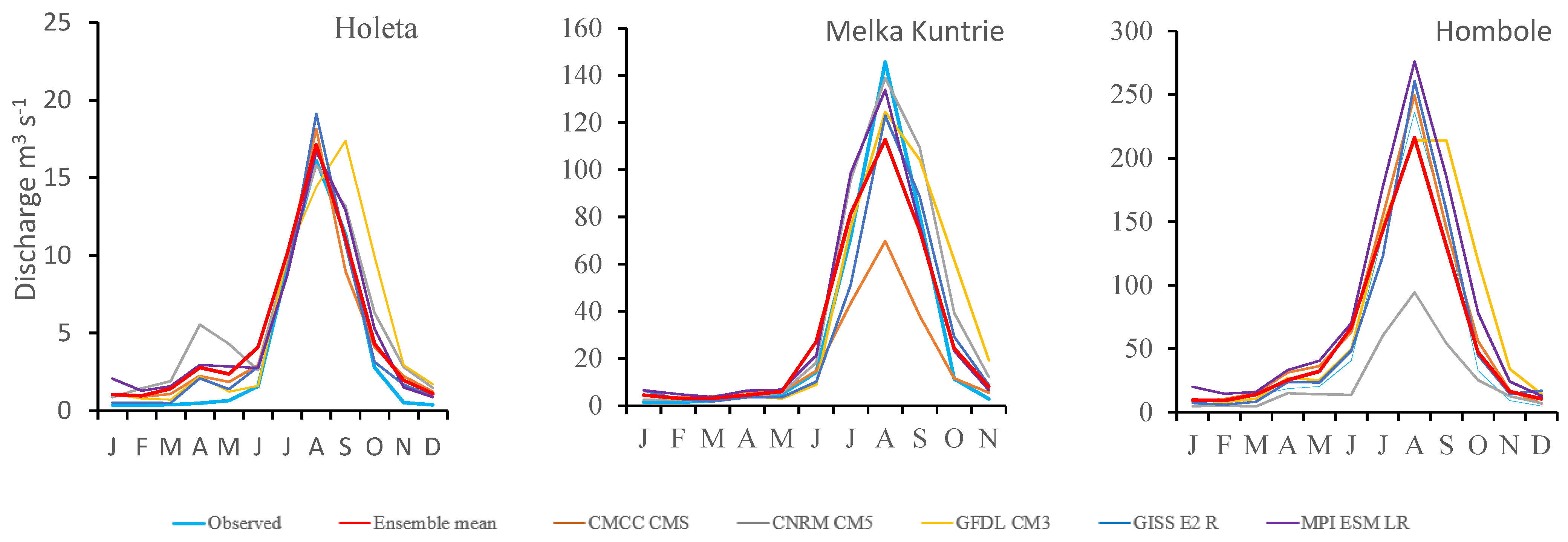
3.1. GCM Simulation Performance

The simulation performance assessment showed that all of the selected GCMs have good simulation capacity over the Upper Awash River Basin. The MREs for GFDLE-CM3, GISS-ET-R, and MPI-ESM-LR are all less than 5% for precipitation and less than 0.55 for temperature. The other GCMs have values of MRE in the range of 7.8% to 42%. The CORR and NSE values for precipitation are all greater than 0.89 and 0.71, respectively. The values of these statistics for air temperatures are similarly high and indicate superior GCM performance than for precipitation [32]; they range between 0.94 and 0.99, and between 0.83 and 0.99, respectively (Appendix A).

3.2. Hydrological Model Calibration and Validation

Calibration and validation of the SWAT model were performed against recorded streamflow data at the six gauging stations (Figure 2). Simulation performance for each gauging station and both the calibration and validation periods is described in Table 5. Performance was satisfactory at the Asigori, Melka Kuntrie, Hombole, and Holeta gauging stations. Performance at Ginchi was relatively poor for the calibration period but good for the validation period. In contrast, the model performed poorly for the Akaki gauging station in both the calibration and validation periods as indicated by the lower R2 and NS values relative to the other gauging stations.

3.3. Changes in Air Temperature

The mean monthly minimum temperature (Tmin) and maximum temperature (Tmax) for the baseline and each GCM, as well as the ensemble mean based on all of the GCMs, are presented in Figure 3 and Figure 4. Across the basin, Tmin for the baseline period ranges between 5.67 and 15.24 °C, while Tmax ranges from 16.70 to 31.06 °C. The mean monthly Tmin for the ensemble means ranges between 7.25 and 16.48 °C, while the corresponding ensemble mean Tmax ranges from 19.10 to 32.65 °C.
The mean annual change in Tmax (°C) and Tmin (°C) for the different GCMs relative to the baseline are presented in Table 6. The baseline (1983–2014) and projected (2015–2100) rate of change of annual Tmax and Tmin, which is defined by Sen’s slope in the MK test, are also presented in Table 7. Both mean annual Tmax and Tmin are projected to increase relative to the baseline at all stations for all five GCMs. Based on the ensemble mean of the GCMs, the change in Tmax across the basin ranges from 1.16 to 1.73 °C, while the Tmin changes range from 0.79 to 2.53 °C. However, individual GCMs project increases in Tmax and Tmin of up to 1.9 and 3.47 °C, respectively (Table 6).
Based on the MK trend tests, an extremely significant (α ≤ 0.001) increasing trend is indicated for both baseline and projected annual Tmax and Tmin (Table 7). The rate of change of temperature for the baseline period ranges from 0.2 to 0.8 °C per decade for both Tmax and Tmin. Projected annual rates of temperature change, however, vary between GCMs. The rate of change of mean annual Tmax is 0.3 °C per decade for CMCC CMS and MPI ESM LR, 0.2 °C per decade for NRM CM5, and 0.1 °C per decade for the GISS E2 R and GISS E2 R GCMs at all stations. The rate of change for mean annual Tmin, on the other hand, is 0.3 °C per decade for CMCC CMS, 0.2 °C per decade for CNRM CM5 and MPI ESM LR, and 0.4 °C per decade for GFDL CM3 and GISS E2 R, again at all stations.

3.4. Changes in Precipitation

Mean annual baseline precipitation for each station and changes (percent) relative to this baseline for the different GCMs and the ensemble mean are presented in Table 8. Increases in mean annual precipitation are indicated in most cases, although GISS E2 R projects decline at five of the six stations (the exception being Hombole). The largest overall increase in mean annual precipitation is projected for Hombole (a 60.5% increase for MPI ESM LR), while the largest decline is at Addis Ababa (14.9%, GISS E2 R).
Annual precipitation trends: The trend analysis revealed that both baseline and projected precipitation changes were not significant at most stations (Table 9). Variation in the magnitude and direction of the rates of changes across the different GCMs was indicated. Ginchi showed a significant (α ≤ 0.05) decreasing trend in precipitation for the baseline (i.e., observed) and a significant (α ≤ 0.05) increasing trend for the GFDL CM3 GCM. Addis Ababa, Alem Tena, Hombole, and Mojo also showed a significant increasing trend in annual precipitation for this GCM. Although they were not significant, there were decreasing trends in annual precipitation at Addis Abba, Alem Tena, and Hombole and increasing trends at Mojo and Tulu Bolo over the baseline period. On the other hand, there were nonsignificant increasing trends projected for CMCC CMS and GFDL CM3 and decreasing trends for GFDL CM3 and MPI ESM LR at all stations. CNRM CM5 also projected a decreasing trend at Ginchi and Addis Ababa and an increasing trend at the remaining stations. The annual ensemble mean trend, on the other hand, showed a nonsignificant decreasing trend at all stations except Tulu Bolo, which indicated a nonsignificant increasing trend.
Seasonal precipitation trends: Although not a significant trend, spring and summer showed a decreasing trend at Ginchi, Alem Tena, and Hombole over the baseline period, while a similarly not significant increasing trend was identified at Mojo and Tulu Bolo over the same period (Table 9). The projected precipitation indicated a decreasing (but not significant) trend in spring and summer for GISS E2 R, in spring for MPI ESM LR and CNRM CM5, and in summer for the GFDL CM3 model at all stations. The ensemble means indicated a nonsignificant decreasing trend in spring and summer and an increasing trend, again, not significant, in autumn and winter at all stations.
Monthly precipitation trends: In the majority of cases, there were nonsignificant (α ≤ 0.05) trends in most of the months at all stations (Figure 5). The five GCMs’ ensemble mean also projected a nonsignificant trend in most months and at most stations. The exception was April for Ginchi (significant decrease), October, and November for Hombole (significant increase).

3.5. Changes in Streamflow

Change in streamflow extremes:Table 10 presents mean discharge (Qmean) (m3 s−1), discharges equaled or exceeded for 5% of the time (Q5) (m3 s−1), and discharges equaled or exceeded for 90% for the time (Q90) (m3 s−1) for each of the five gauging stations for the baseline as well as the changes (percent) from these baseline figures for each GCM and the ensemble mean. Following the approach of [59], Qmean, Q5, and Q90 were derived from monthly baseline and projected discharge time series data. The annual and seasonal streamflow trends for each gauging station for each of the GCMs and the ensemble mean are described in Table 11.
The projected Qmean at Ginchi and Holeta show an increase for all five GCMs and the ensemble mean. In contrast, Akaki Qmean shows a decrease for all GCMs except CNRM CM5. Asigori and Kuntrie, on the other hand, show a decrease for CMCC CMS and GISS E2 R and an increase for CNRM CM5, GFDL CM3, and MPI ESM LR. Qmean at Hombole shows an increase for all GCMs except CNRM CM5. The largest increase in Qmean is projected in the upper catchment at Ginchi (198.3% for MPI ESM LR), while the largest decrease (55.2% for CNRM CM5) is projected in the lower catchment at Hombole. The ensemble mean projects an increase at all stations except Akaki.
All GCMs project increases in streamflow during periods of high flow (i.e., Q5) at Ginchi and Holeta and decreases at Asigori and Akaki. Q5 declines at Kuntrie for CMCC CMS and increases for the remaining GCMs. Results for Hombole, on the other hand, show declines in high flows for CMCC CMS, CNRM CM5, and GFDL CM3 and increases for GISS E2 R and MPI ESM LR. Q5 for the ensemble mean indicates declines during the high flow period at all stations except Ginchi. Low streamflow (i.e., Q90) increases at Holeta and decreases at Akaki and Hombole. Q90 at Kuntrie, on the other hand, increases for CMCC CMS, CNRM CM5, and MPI ESM LR and decreases for GFDL CM3 and GISS E2 R. Q90 for the ensemble mean declines at Akaki and increases at Holeta, Kuntrie, and Hombole catchments.
Annual streamflow trends: The annual baseline streamflow trends (Table 11) reveal increasing discharge at Melka Kuntrie, Hombole, and Akaki, while decreasing trends are evident at Ginchi, Asigori, and Holeta. However, only Melka Kuntrie showed a statistically significant increasing trend (6.9 m3 s−1 per decade). In common with projected precipitation and temperature, there is no overall agreement on the projected trends in both the magnitude and direction of change for streamflow across the GCMs (Table 11). Based on individual GCM projections, significant increasing trends in annual mean discharge were identified at Ginchi (6.3 m3 s−1 per decade), Holeta (2.1 m3 s−1 per decade), Asigori (3.0 m3 s−1 per decade), Akaki (8.3 m3 s−1 per decade), Hombole (25.7 m3 s−1 per decade), and Melka Kuntrie (13.5 m3 s−1 per decade) for GFDL CM3. Similarly, the MPI ESMLR GCM projects significant increasing trends at Ginchi (3.6 m3 s−1 per decade), Asigori (2.2 m3 s−1 per decade), Hombole (17.5 m3 s−1 per decade), and Melka Kuntrie (7.7 m3 s−1 per decade). In contrast, GISS E2 R projects nonsignificant but decreasing trends at these stations. The annual trends for the ensemble mean were not significant at all of the gauging stations.
Seasonal streamflow trends: Most of the seasonal trends for the baseline period were not significant; significant trends were restricted to an increasing trend (20.7 m3 s−1 per decade) for summer at Melka Kuntrie, a decreasing trend (6.5 m3 s−1 per decade) for autumn at Ginchi, and an increasing annual trend (6.9 m 3 s−1 per decade) at Melka Kuntrie. Similarly, the projected streamflows showed a nonsignificant increasing trend for most of the GCMs. However, a significant increasing trend was observed in spring at Ginchi (3.4 m3 s−1 per decade), Holeta (0.1 m3 s−1 per decade), Asigori (0.3 m3 s−1 per decade), Akaki (0.8 m3 s−1 per decade), Hombole (1.9 m3 s−1 per decade), and Melka Kuntrie (0.4 m3 s−1 per decade) for GFDL CM3. Furthermore, summer showed a significant increasing trend at Ginchi (3.5 m3 s−1 per decade), Holeta (0.2 m3 s−1 per decade), Asigori (0.4 m3 s−1 per decade), Akaki (1.0 m3 s−1 per decade), Hombole (3.1 m3 s−1 per decade), and Melka Kuntrie (1.4 m3 s−1 per decade) for MPI ESMLR. For the ensemble mean, winter experiences a significant increasing trend at Ginchi and Asigori (at rates of 0.12 m 3 s−1 and 0.029 m 3 s−1 per decade, respectively), while autumn has a significant increasing trend at Asigori (0.091 m 3 s−1 per decade). On the other hand, there is a significant decline in spring at Hombole (−0.58 m 3 s−1 per decade).
Monthly streamflow trends: The monthly trends for baseline streamflow shows nonsignificant decreases at Ginchi, Asigori, and Holeta and increases at Akaki, Hombole, and Melka Kuntrie in most months (Figure 6). However, Ginchi experienced a significant decrease in September (8.2 m3 s−1 per decade), November (0.1 m3 s−1 per decade), and December (0.1 m3 s−1 per decade). In contrast, Akaki, Hombole, and Melka experienced a significant increasing trend in January (2.0 m3 s−1, 1.6 m3 s−1, and 0.5 m3 s−1 per decade, respectively) and November (1.7 m3 s−1, 3.1 m3 s−1, and 0.9 m3 s−1 per decade, respectively). Melka Kuntrie also showed a significant increasing trend in May, June, July, and December (1.1 m3 s−1, 0.6 m3 s−1, 4.5 m3 s−1, 29.6 m3 s−1, and 0.6 m3 s−1 per decade, respectively).
The ensemble mean projects a significant increase at Ginchi in January (0.1 m3 s−1 per decade) and December (0.1 m3 s−1 per decade). In contrast, there is a significant decreasing trend at Holeta in April and July (rates of −0.01 m3 s−1 and −0.03 m3 s−1 per decade, respectively). Significant increasing trends (0.1 m3 s−1 per decade) are projected at Asigori from September to January, while significant decreasing trends are projected for April and July (0.1 m3 s−1 and 0.3 m3 s−1 per decade, respectively). At both Akaki and Melka Kuntrie, the ensemble mean projects significant increasing trends for October and July (0.2 m3 s−1 and 1.2 m3 s−1 per decade), while at Hombole significant decreasing trends are projected for April (1.2 m3 s−1 per decade) and July (3.3 m3 s−1 per decade).

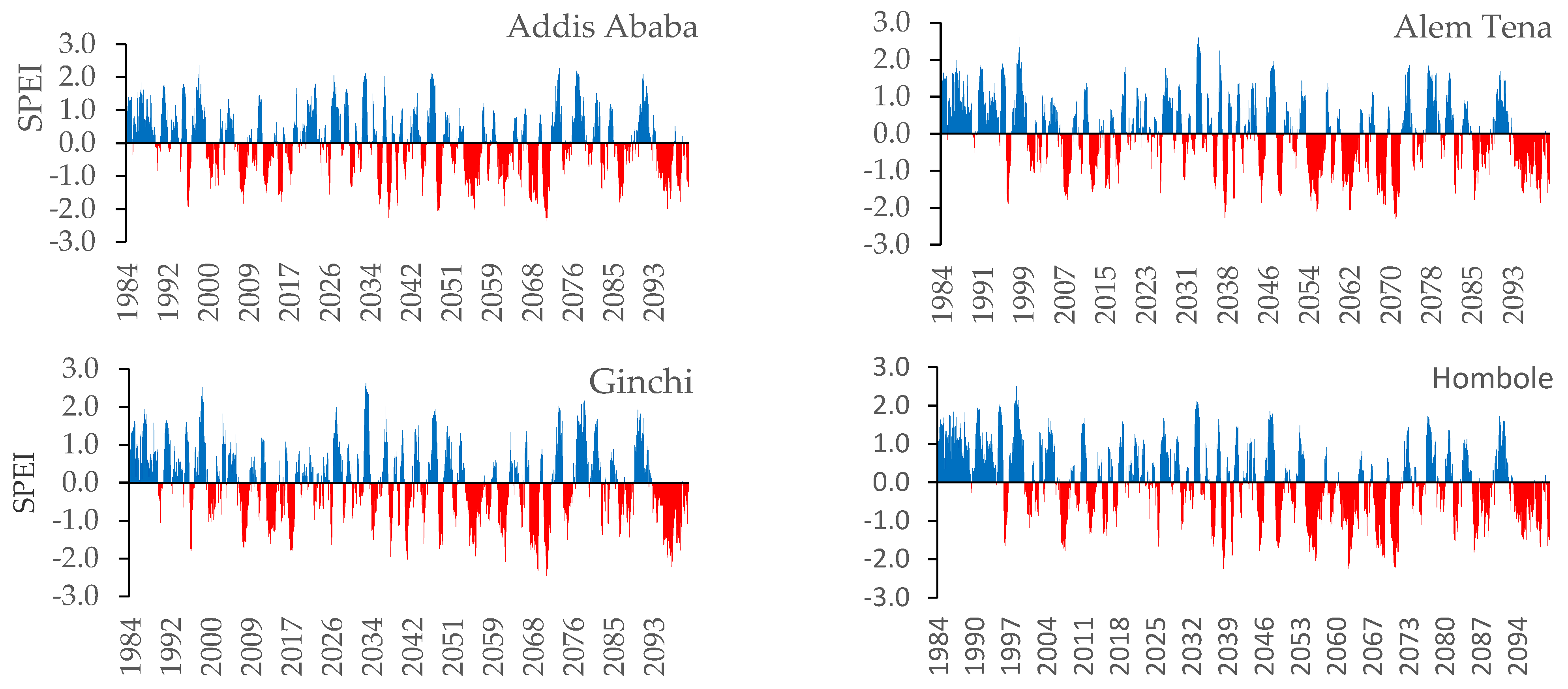
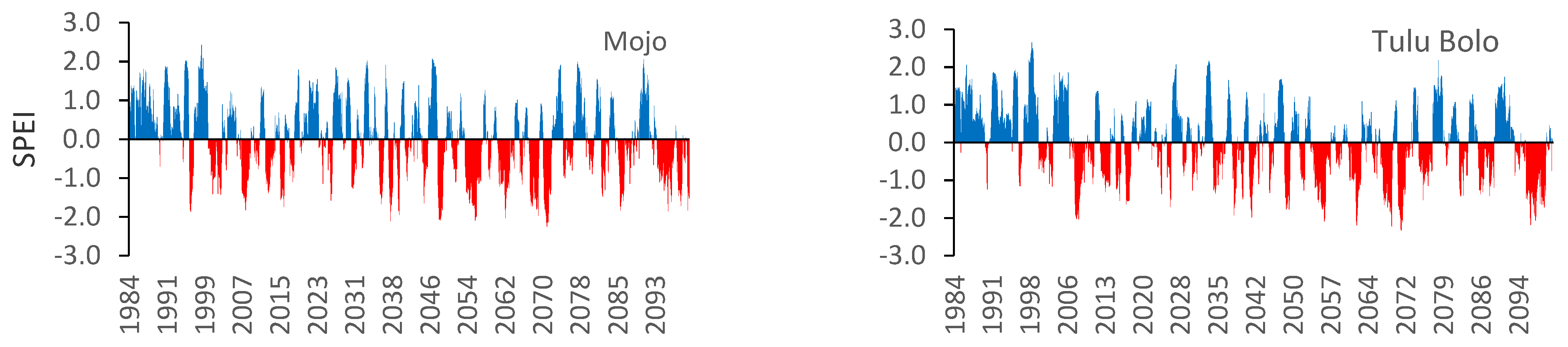
3.6. Climate Drought Index

Using the historical climate data (1984–2020) and the five GCM ensemble mean projections (2021–2100), the historical and potential future climatic droughts were analyzed for each meteorological station using the SPEI at a time scale of 12 months (Figure 7). Accordingly, the SPEI for the historical period shows that the years 1996, 1997, 2007, 2008, 2013, 2014, 2016, and 2018 were very dry, while 1999 was a very wet year. Figure 8 clearly shows an increasing trend towards meteorological drought in recent decades (2006–2020) compared with the beginning of the period (1984–1994). The SPEI trend analysis demonstrates a decrease towards a negative value at all stations. This trend was statistically significant at α ≤ 0.01, confirming the increasing tendency towards meteorological drought.
The projected SPEI for the period 2021–2100 indicates an increase in the frequency and severity of drought especially for the period 2045–2072 compared with 2021–2047. The increasing drought trend is significant (α ≤ 0.01) at all stations.

3.7. Hydrological Drought Index

The historical SDI is dominated by negative values, indicating dry years at most of the stations, the exception being Akaki (Figure 8). The basin experienced a range of conditions from modestly dry to very severe hydrological drought between 1986 and 2005. The MK trend test confirmed a significant increasing trend towards negative values of SDI at Ginchi, Asigori, Holeta, and Melka Kuntrie, supporting the assertation of increasing hydrological drought over the past three decades. However, a significant increasing trend towards positive values (indicating wetter conditions) was identified for Akaki, while no significant trend was established for Hombole.
The projected SDI, on the other hand, indicates conditions that range from modestly dry to modestly wet at all stations. The MK trend analysis confirmed an increasing trend towards positive values (i.e., wetter years) at all stations. Trends were statistically significant at Asigori, Ginchi, and Akaki.

4. Discussion

4.1. The Impacts of Climate Change on Precipitation

This study suggests that some changes in the climate of the Upper Awash River Basin have occurred over the period beginning in 1984 and extending to 2014. Declines in precipitation in spring and summer and increases in autumn and winter were identified over this baseline period, although these trends were not statistically significant. Results show that at some stations precipitation decreased by up to 22.4 and 8.8 mm per decade in spring and summer, respectively, between 1983 and 2014. This study, therefore, supports earlier investigations regarding the impacts of climate change on precipitation and their implication for Ethiopia [60,61,62,63,64]. For instance, a study in the southern part of the country revealed that precipitation in spring and summer declined between 1972 and 2011 [65]. In another study in the northeastern part of the Blue Nile basin, a nonsignificant decreasing trend was observed in spring between 1981 and 2010 [66]. A further study also showed a decreasing trend in precipitation in spring throughout the country between 1980 and 2010 [67].
The IPCC third assessment report [2] stated that because of the diversity of climatic conditions and limited meteorological stations, projected precipitation in Africa, particularly at regional and local scales, is not well defined. Under intermediate warming scenarios, one study showed an increase in projected rainfall during the dry season (December to February) and a decrease in the rainy season (June to August) over parts of East Africa, including the current study area [2]. This study showed that for the ensemble mean, projected future precipitation, especially in spring and summer and as a result annually, showed a decreasing trend at most stations. The magnitude and directions of change do, however, vary between different GCMs, stations, and seasons, echoing the variability identified in earlier studies employing a number (in most cases, fewer than the current study) of climate models [20,21,67].
Declining precipitation will have a significant implication for agricultural productivities. As one of the major agricultural regions of Ethiopia, spring and summer are overwhelmingly important in the Upper Awash River Basin because more than 95% of crop production is produced at this time of year [68]. Decreases in precipitation together with the extremely variable nature of rainfall, and increasing temperature, are likely to have a significant impact on agricultural production as well as the water sector of the basin. Furthermore, the economic dependency of both rural and urban communities on agriculture, combined with the dominant rain-fed nature of the farming system, makes the area particularly vulnerable to climate variability and change. It has been suggested that climate change would affect Ethiopia’s GDP growth by 0.5–2.5% per year due to declining agricultural productivity [69]. Another study showed that, due to rainfall variability, about USD 2 billion will be lost in the agricultural sector over future decades [70].

4.2. The Implication of Climate Change on Streamflow

Streamflow is strongly influenced by changes in precipitation, temperature, land use, and other factors, such as the withdrawal of water for human use. Change in streamflow can affect the amount of water available for irrigation, water supply, and hydropower generation. Seasonal and spatial variability of streamflow and their changes into the future, therefore, have the potential to exert significant impacts on the economy and local development. The area downstream of the Upper Awash River Basin is relatively developed for irrigation. These irrigation developments include the Wonji and Metehara sugar plantations; upper, middle, and lower Awash state farms developed for fruit and vegetable production; and cotton plantations. Such schemes have flourished following the construction of the Koka Dam, which defines the outlet of the current study area [71]. Streamflow changes in the upper catchment will have an impact on reservoir inflows, and they, therefore, have the potential for large impacts on downstream projects.
This study suggests that discharges during the high flow period (as indicated by Q5) decline by up to 61.9% compared with the baseline at some gauging stations with the largest changes in the opposite direction indicating increases of 84.3%. The ensemble mean, however, projects a decline in these flows at five of the stations (mean of those declining = −40.8%). Conversely, mean flows for the ensemble mean are projected to increase at five stations (declines at the one remaining station), although there is a notable decline in the magnitude of the increases in a downstream direction (just 1.4% at the lowest station). Across the different GCMs, there is considerable variability in the magnitude of changes in mean flow, including both increases and decreases, which concur with those results of other multi-GCM studies of change over the basin [22]. The low flow period is projected to experience both declines and increases in discharge with Q90 reducing by 100% (i.e., flows cease) at Akaki and Hombole for individual GCM projections (Table 10). The magnitude of changes in percentage terms is much higher for low flows than both mean and high flows. These larger percentage changes in low flows agree with an earlier study undertaken within the Upper Awash Basin using a number of GCMs, including some used in the current study [22]. It also supports a recent global analysis showing greater risks of change in low flow conditions compared with high flows [72]. However, for the ensemble mean there are more declines in high flows than in low flows across the different gauging stations. Reductions in streamflow during the high flow period results from precipitation reductions in spring and summer, the main rainy seasons in the basin. A similar study in the Blue Nile basin identified declines in low streamflow (Q95) of 18.1% between 1982 and 2000, while high streamflow (Q5) increased by 7.6% over the same period [73].
The trend analysis also confirmed that streamflow in the upper catchment (Ginchi, Asigori, and Holeta gauging stations) experienced a decline over the period 1985–2010, while it increased in the lower catchment (Akaki, Melka Kuntrie, and Hombole) in most months and seasons. The projected streamflow, on the other hand, showed no overall agreement in terms of both magnitude and direction of change between different GCMs. As an example, GISS E2 R showed a dominant decreasing trend, while GFDL CM3 projected an increasing trend in most months at Ginchi, Asigori, Hombole, and Kuntrie. CMCC CMS projected a nonsignificant increasing trend, while for MPI ESMLR there was a significant increasing trend in most of the months at all stations. The ensemble mean showed an increasing monthly trend from September to February and a decreasing trend in April and July. The seasonal results showed a decreasing trend in spring and summer, while an increasing trend was identified for autumn and winter. At an annual level, results indicated a decreasing trend at Holeta and Hombole and an increasing trend at the remaining stations.

4.3. The Implication of Climate Change on Meteorological and Hydrological Drought

Changes in temperature and precipitation can exacerbate extreme events, such as meteorological and hydrological droughts. Drought is a common phenomenon that occurs frequently in many parts of Ethiopia, including the study area. The frequency of drought in the country has increased, and devastating droughts have occurred in the recent decade [74,75]. The historical meteorological drought index used in the current study indicated an extremely significant increasing trend across the basin (Figure 8). The projected drought index also suggested that the basin will experience more severe droughts over the current century. Many studies have stated that droughts in Ethiopia are El Niño induced and that this climatic phenomenon is responsible for extreme dryness and major rainfall failures in many parts of the country [21,64,71,72]. Historical droughts have been associated with severe water and food shortages, widespread hunger, and diseases that destroyed the livelihood of millions of people across a large part of Ethiopia [74]. With the projected increase in drought incidence and severity, these extreme conditions are likely to remain significant concerns in the country. The hydrological drought index, on the other hand, showed significant dry years at Asigori and Holeta and very wet years at Ginchi, Akaki, and Melka Kuntrie between 1985 and 2020. In contrast, the projected SDI indicated that more wet years are expected than dry years.

5. Conclusions

This study demonstrated that over the baseline period (1983–2014), the Upper Awash River Basin experienced increases in mean annual maximum temperature (Tmax) in the ranges of 0.60 to 1.90 °C, while mean annual minimum temperature (Tmin) increased between 0.63 and 3.47 °C. The rate of change of temperature for the baseline period ranges from 0.2 to 0.8 °C per decade for both Tmax and Tmin. The projected annual rate of change in temperature over the remainder of the current century varies in magnitude between the five GCMs (between 0.1 and 0.4 °C per decade).
The trend analysis for precipitation shows a decreasing trend over the baseline period for most of the stations. Mean annual precipitation is projected to increase at all stations for all GCMs except GISS ET R. The overall range of change across all GCMs and stations is −14.9% to 60.0%. There is notable variation in the magnitude and direction of change in monthly, seasonal, and annual precipitation across the different GCMs. In the majority of cases, there were nonsignificant (α ≤ 0.05) trends for most months at all stations. The ensemble mean based on the five GCMs also projected a nonsignificant trend in most months and at most stations. However, both baseline and projected precipitation showed a decrease in spring and summer and increases in autumn and winter.
Based on projections using the ensemble mean, streamflow declines during the high flow period at all stations except Ginchi. On the other hand, low flows decrease at Akaki and increase at Holeta, Kuntrie, and Hombole. The mean annual streamflow trend shows an increase at all stations except Akaki. Individual GCMs, however, project changes that differ in terms of both magnitude and direction. Changes range from a decrease of 55% (Hombole for CNRM CM5) and an increase of 198% (Ginchi for MPI ESM LR). Streamflow during wet and dry periods also showed an increase at Ginchi, Holeta, and Kuntrie and a decrease at Asigori, Holeta, and Hombole. The baseline and projected mean monthly, seasonal, and annual streamflow trends indicated a nonsignificant decrease at Ginchi, Asigori, and Holeta and an increase at Akaki, Hombole, and Melka Kuntrie. There was no agreement over the projected streamflow trend in terms of both the magnitude and direction across the different GCMs. The GISS E2 R GCM projected a decreasing trend, while other GCMs projected an increasing trend in most months at all stations. Statistically, the CMCC CMS, CNRM CM5, and GISS E2 R GCMs showed a nonsignificant trend, while the GFDL CM3 and MPI ESMLR GCMs indicated a significant increasing trend at all stations. The seasonal ensemble mean streamflow, however, showed a decreasing trend in spring and summer at all stations except Asigori. The ensemble mean also showed a decrease at Holeta and Hombole and an increase at the remaining stations.
The SPEI confirmed that the basin experienced significant droughts in the past, and the frequency and severity of drought will increase in the future. The historical SDI, on the other hand, showed hydrological drought at Asigori and Holeta and very wet years at the remaining stations. The trend of the projected SDI showed more wet years than dry years.
Climate change in the basin would create seasonal variation in precipitation and streamflow. Both precipitation and streamflow will decline in the wet seasons and increase in the dry seasons. These changes are likely to have an impact on the agricultural system and water resource use within the basin. As such, there will be an urgent need to develop mitigation approaches in response to changing hydrometeorological conditions.
This research work is based on five GCMs and the intermediate emission scenarios. The extension of the research could include additional GCMs and emission scenarios to expand the assessment of the impacts of climate change on the hydrology of the Upper Awash Basin.

Author Contributions

Conceptualization, N.C.E., J.W.R., J.R.T., A.B. and D.S.; methodology, N.C.E., J.W.R., J.R.T., A.B., E.A., A.M. and G.M.M.; software, N.C.E., J.W.R., J.R.T., A.B., E.A., A.M., T.D.D. and P.M.O.; validation, N.C.E., J.W.R., J.R.T., A.B., E.A. and A.M.; formal analysis, N.C.E., J.W.R., J.R.T., A.B., E.A., A.M., T.D.D. and G.M.M.; investigation, N.C.E., J.W.R., J.R.T., A.B., E.A., A.M. and T.D.D.; resources, N.C.E., J.W.R., J.R.T., A.B., E.A., A.M., T.D.D. and D.S.; data curation, N.C.E., J.W.R., J.R.T., A.B., E.A., A.M., T.D.D., M.B.M. and G.M.M.; writing—original draft preparation, N.C.E., J.W.R., J.R.T., A.B., E.A., A.M., T.D.D., P.M.O., J.H., M.B.M. and G.M.M.; writing—review and editing, N.C.E., J.W.R., J.R.T., A.B., E.A., A.M., T.D.D., P.M.O., J.H., M.B.M., G.M.M. and D.S.; visualization, N.C.E., J.W.R., J.R.T., A.B., E.A., A.M., J.H., M.B.M., G.M.M. and D.S.; supervision, J.W.R., J.R.T., E.A., A.M., T.D.D., P.M.O., J.H., M.B.M., G.M.M. and D.S.; project administration, J.W.R., J.R.T., E.A., A.M., T.D.D., P.M.O., J.H., M.B.M., G.M.M. and D.S.; funding acquisition, N.C.E., J.W.R., J.R.T., A.B., E.A., A.M., T.D.D., P.M.O., J.H., M.B.M., G.M.M. and D.S. All authors have read and agreed to the published version of the manuscript.

Funding

This research was financially supported through CCAFS-EC grant reference 2000002575 for the project Building Livelihoods and Resilience to Climate Change in East and West Africa: Agricultural Research for Development (AR4D) for large-scale implementation of Climate-Smart Agriculture. The funds are administered by the International Fund for Agricultural Development (IFAD), Rome, Italy, while the project is implemented by Alliance Bioversity-CIAT. The initial stages of the research were financially supported by the UK Department for International Development (DfID) and the Climate Impact Research Capacity and Leadership Enhancement (CIRCLE) program (grant number 201871). The final part of the study was financially supported through a grant from the World Bank “Accelerating Impacts of CGIAR Climate Research for Africa (AICCRA)” ESA regional project (Grant number D7540) signed between CIAT and the International Development Association (IDA).

Institutional Review Board Statement

Not applicable.

Informed Consent Statement

Not applicable.

Data Availability Statement

The data presented in this study are available on request from the corresponding author. The data are not publicly available due to confidentiality requirements of the funding organisations for the project.

Acknowledgments

The authors would like to thank the Ethiopian National Meteorological Agency; Ministry of Irrigation, Energy, and Water Resource of Ethiopia; and Global Runoff Data Centre for providing the required climate and streamflow data.

Conflicts of Interest

The authors declare no conflict of interest. The funders had no role in the design of the study; in the collection, analyses, or interpretation of data; in the writing of the manuscript; or in the decision to publish the results.

Appendix A

Table A1. Simulation performance of different GCMs.
StationGCM ModelsPrecipitationTemperature
MRECORNSEMRECORNSE
Addis
Ababa
CMCC_CMS1.430.990.990.0020.990.99
CNRM-CM54.290.990.980.0000.990.99
GFDL-CM3−0.720.970.940.0090.990.99
GISS-ET-R−1.360.990.98−0.3500.970.95
MPI-ESM-LR1.160.910.840.0000.990.99
Alem Tena CMCC_CMS2.400.990.980.0020.990.99
CNRM-CM51.810.970.95−0.0040.990.99
GFDL-CM30.470.990.97−0.0070.990.99
GISS-ET-R−0.160.990.98−0.3170.970.93
MPI-ESM-LR1.810.890.800. 0000.990.99
Ginchi CMCC_CMS7.180.990.980.0020.990.99
CNRM-CM58.040.990.98−1.2240.990.99
GFDL-CM35.480.980.97−0.0420.990.99
GISS-ET-R4.250.990.97−0.3870.990.99
MPI-ESM-LR8.670.940.880.0000.990.99
HomboleCMCC_CMS42.200.990.710. 0000.990.99
CNRM-CM542.210.990.710.0020.990.99
GFDL-CM342.200.990.710.1370.990.99
GISS-ET-R42.200.990.71−0.3140.980.94
MPI-ESM-LR42.160.990.710.0100.990.99
MojoCMCC_CMS1.460.980.970.0000.990.99
CNRM-CM53.450.990.980.0060.990.99
GFDL-CM3−0.260.970.940.0240.660.32
GISS-ET-R−1.750.980.97−0.3130.980.95
MPI-ESM-LR0.900.910.830.0100.990.99
Tulu BoloCMCC_CMS8.380.990.970.0030.990.99
CNRM-CM58.600.990.970.0030.990.99
GFDL-CM34.460.990.98−0.0190.990.99
GISS-ET-R4.780.980.97−0.3510.940.83
MPI-ESM-LR10.200.950.890.0000.990.99

References

  1. Serdeczny, O.; Adams, S.; Baarsch, F.; Coumou, D.; Robinson, A.; Hare, W.; Schaeffer, M.; Perrette, M.; Reinhardt, J. Climate change impacts in Sub-Saharan Africa: From physical changes to their social repercussions. Reg. Environ. Chang. 2017, 17, 1585–1600. [Google Scholar] [CrossRef]
  2. Cooper, R.N.; Houghton, J.T.; McCarthy, J.J.; Metz, B. Climate Change 2001: The Scientific Basis. Foreign Aff. 2002, 81, 208. [Google Scholar] [CrossRef]
  3. Intergovernmental Panel on Climate Change (IPCC). Summary for Policymakers. In Global Warming of 1.5 °C; Intergovernmental Panel on Climate Change: Geneva, Switzerland, 2018; pp. 1–24. [Google Scholar]
  4. Intergovernmental Panel on Climate Change (IPCC). Climate Change 2014: Synthesis Report. Contribution of Working Groups I, II and III to the Fifth Assessment Report of the Intergovernmental Panel on Climate Change; Intergovernmental Panel on Climate Change: Geneva, Switzerland, 2014. [Google Scholar]
  5. Faramarzi, M.; Abbaspour, K.C.; Vaghefi, S.A.; Farzaneh, M.R.; Zehnder, A.J.; Srinivasan, R.; Yang, H. Modeling impacts of climate change on freshwater availability in Africa. J. Hydrol. 2013, 480, 85–101. [Google Scholar] [CrossRef]
  6. Schuol, J.; Abbaspour, K.C.; Srinivasan, R.; Yang, H. Estimation of freshwater availability in the West African sub-continent using the SWAT hydrologic model. J. Hydrol. 2008, 352, 30–49. [Google Scholar] [CrossRef]
  7. Almazroui, M.; Saeed, F.; Saeed, S.; Islam, M.N.; Ismail, M.; Klutse, N.A.B.; Siddiqui, M.H. Projected Change in Temperature and Precipitation over Africa from CMIP6. Earth Syst. Environ. 2020, 4, 455–475. [Google Scholar] [CrossRef]
  8. Engelbrecht, F.; Adegoke, J.; Bopape, M.-J.; Naidoo, M.; Garland, R.; Thatcher, M.; McGregor, J.; Katzfey, J.; Werner, M.; Ichoku, C.; et al. Projections of rapidly rising surface temperatures over Africa under low mitigation. Environ. Res. Lett. 2015, 10, 085004. [Google Scholar] [CrossRef]
  9. Arnell, N.W.; Brown, S.N.; Gosling, S.; Gottschalk, P.; Hinkel, J.; Huntingford, C.; Lloyd-Hughes, B.; Lowe, J.A.; Nicholls, R.J.; Osborn, T.J.; et al. The impacts of climate change across the globe: A multi-sectoral assessment. Clim. Chang. 2014, 134, 457–474. [Google Scholar] [CrossRef] [Green Version]
  10. Mekonnen, D.F.; Disse, M. Analyzing the future climate change of Upper Blue Nile River basin using statistical downscaling techniques. Hydrol. Earth Syst. Sci. 2018, 22, 2391–2408. [Google Scholar] [CrossRef] [Green Version]
  11. Gadissa, T.; Nyadawa, M.; Behulu, F.; Mutua, B. The Effect of Climate Change on Loss of Lake Volume: Case of Sedimentation in Central Rift Valley Basin, Ethiopia. Hydrology 2018, 5, 67. [Google Scholar] [CrossRef] [Green Version]
  12. Jilo, N.B.; Gebremariam, B.; Harka, A.E.; Woldemariam, G.W.; Behulu, F. Evaluation of the Impacts of Climate Change on Sediment Yield from the Logiya Watershed, Lower Awash Basin, Ethiopia. Hydrology 2019, 6, 81. [Google Scholar] [CrossRef] [Green Version]
  13. Legesse, D.; Abiye, T.A.; Vallet-Coulomb, C.; Abate, H. Streamflow sensitivity to climate and land cover changes: Meki River, Ethiopia. Hydrol. Earth Syst. Sci. 2010, 14, 2277–2287. [Google Scholar] [CrossRef] [Green Version]
  14. Hailemariam, K. Impact of climate change on the water resources of Awash River Basin, Ethiopia. Clim. Res. 1999, 12, 91–96. [Google Scholar] [CrossRef] [Green Version]
  15. Abdo, K.S. Assessment of Climate Change Impacts on the Hydrology of Gilgel Abay Catchment in Lake Tana Basin, Ethiopia. Master’s Thesis, International Institute for Geo-Information Science and Earth Observation, Enschede, The Netherlands, 2009. [Google Scholar]
  16. Zeray, L.; Roehrig, J.; Alamirew, D.; Abiyata, L.; Shala, L. Climate Change Impact on Lake Ziway Watershed Water. Unpublished. Master’s Thesis, Institute for Technology in the Tropics, University of Applied Science, Cologne, Germany, 2006. [Google Scholar]
  17. Abdo, K.S.; Fiseha, B.M.; Rientjes, T.H.M.; Gieske, A.S.M.; Haile, A.T. Assessment of climate change impacts on the hydrology of Gilgel Abay catchment in Lake Tana Basin, Ethiopia. Hydrol. Process. 2009, 23, 3661–3669. [Google Scholar] [CrossRef]
  18. Taddese, G.; Sonder, K.; Peden, D. The Water of the Awash River Basin: A Future Challenge to Ethiopia; ILRI: Addis Ababa, Ethiopia, 2009. [Google Scholar]
  19. Daba, M.; Tadele, K.; Shemalis, A. Evaluating Potential Impacts of Climate Change on Surface Water Resource Availability of Upper Awash Sub-Basin, Ethiopia. Open Water J. 2015, 3, 22. [Google Scholar]
  20. Daba, M.; You, S. Assessment of Climate Change Impacts on River Flow Regimes in the Upstream of Awash Basin, Ethiopia: Based on IPCC Fifth Assessment Report (AR5) Climate Change Scenarios. Hydrology 2020, 7, 98. [Google Scholar] [CrossRef]
  21. Taye, M.T.; Dyer, E.; Hirpa, F.A.; Charles, K. Climate Change Impact on Water Resources in the Awash Basin, Ethiopia. Water 2018, 10, 1560. [Google Scholar] [CrossRef] [Green Version]
  22. Chan, W.C.H.; Thompson, J.R.; Taylor, R.G.; Nay, A.E.; Ayenew, T.; MacDonald, A.M.; Todd, M.C. Uncertainty assessment in river flow projections for Ethiopia’s Upper Awash Basin using multiple GCMs and hydrological models. Hydrol. Sci. J. 2020, 65, 1720–1737. [Google Scholar] [CrossRef]
  23. Neitsch, S.; Arnold, J.; Kiniry, J.; Williams, J. Soil & Water Assessment Tool Theoretical Documentation Version 2009; Texas Water Resources Institute: College Station, TX, USA, 2011; pp. 1–647. [Google Scholar]
  24. Abbaspour, K.C.; Vaghefi, S.A.; Srinivasan, R. A Guideline for Successful Calibration and Uncertainty Analysis for Soil and Water Assessment: A Review of Papers from the 2016 International SWAT Conference. Water 2017, 10, 6. [Google Scholar] [CrossRef] [Green Version]
  25. Shrestha, M.; Acharya, S.C.; Shrestha, P.K. Bias correction of climate models for hydrological modelling—Are simple methods still useful? Meteorol. Appl. 2017, 24, 531–539. [Google Scholar] [CrossRef] [Green Version]
  26. Hughes, D.A.; Mantel, S.; Mohobane, T. An assessment of the skill of downscaled GCM outputs in simulating historical patterns of rainfall variability in South Africa. Hydrol. Res. 2013, 45, 134–147. [Google Scholar] [CrossRef]
  27. Raju, K.S.; Kumar, D.N. Review of approaches for selection and ensembling of GCMs. J. Water Clim. Chang. 2020, 11, 577–599. [Google Scholar] [CrossRef]
  28. Changulaa, L.K.; Jarvisa, J. Use of the Multi-Model Ensemble Mean of Global Climate Models for Hydroelectricity Generation Planning in Zambia. In Proceedings of the 38th Annual Conference of the International Association for Impact Assessment, Durban, South Africa, 16–19 May 2018. [Google Scholar]
  29. Thomson, A.M.; Calvin, K.V.; Smith, S.J.; Kyle, G.P.; Volke, A.; Patel, P.; Delgado-Arias, S.; Bond-Lamberty, B.; Wise, M.A.; Clarke, L.E.; et al. RCP4.5: A pathway for stabilization of radiative forcing by 2100. Clim. Chang. 2011, 109, 77–94. [Google Scholar] [CrossRef] [Green Version]
  30. Hassan, I.; Kalin, R.M.; White, C.J.; Aladejana, J.A. Selection of CMIP5 GCM Ensemble for the Projection of Spatio-Temporal Changes in Precipitation and Temperature over the Niger Delta, Nigeria. Water 2020, 12, 385. [Google Scholar] [CrossRef] [Green Version]
  31. Wilby, R.L.; Charles, S.P.; Zorita, E.; Timbal, B.; Whetton, P.; Mearns, L.O. Guidelines for Use of Climate Scenarios Developed from Statistical Downscaling Methods. Analysis 2004, 27, 1–27. [Google Scholar]
  32. Zhu, Y.; Lin, Z.; Wang, J.; Zhao, Y.; He, F. Impacts of Climate Changes on Water Resources in Yellow River Basin, China. Procedia Eng. 2016, 154, 687–695. [Google Scholar] [CrossRef] [Green Version]
  33. Wilby, R.; Dawson, C.; Murphy, C.; O’Connor, P.; Hawkins, E. The Statistical DownScaling Model-Decision Centric (SDSM-DC): Conceptual basis and applications. Clim. Res. 2014, 61, 259–276. [Google Scholar] [CrossRef] [Green Version]
  34. Mearns, M.; Giorgi, L.O.; Whetton, F.; Pabon, P.; Hulme, D.; Lal, M. Guidelines for Use of Climate Scenarios Developed from Regional Climate Model Experiments; Data Distribution Centre of the Intergovernmental Panel on Climate Change: Geneva, Switzerland, 2003. [Google Scholar]
  35. Teutschbein, C.; Seibert, J. Bias correction of regional climate model simulations for hydrological climate-change impact studies: Review and evaluation of different methods. J. Hydrol. 2012, 456–457, 12–29. [Google Scholar] [CrossRef]
  36. Fang, G.H.; Yang, J.; Chen, Y.N.; Zammit, C. Comparing bias correction methods in downscaling meteorological variables for a hydrologic impact study in an arid area in China. Hydrol. Earth Syst. Sci. 2015, 19, 2547–2559. [Google Scholar] [CrossRef] [Green Version]
  37. Vicente-Serrano, S.M.; Beguería, S.; López-Moreno, J.I. A Multiscalar Drought Index Sensitive to Global Warming: The Standardized Precipitation Evapotranspiration Index. J. Clim. 2010, 23, 1696–1718. [Google Scholar] [CrossRef] [Green Version]
  38. Nalbantis, I.; Tsakiris, G. Assessment of Hydrological Drought Revisited. Water Resour. Manag. 2009, 23, 881–897. [Google Scholar] [CrossRef]
  39. Zeng, X.; Zhao, N.; Sun, H.; Ye, L.; Zhai, J. Changes and Relationships of Climatic and Hydrological Droughts in the Jialing River Basin, China. PLoS ONE 2015, 10, e0141648. [Google Scholar] [CrossRef] [Green Version]
  40. Hirsch, R.M.; Slack, J.R. A Nonparametric Trend Test for Seasonal Data with Serial Dependence. Water Resour. Res. 1984, 20, 727–732. [Google Scholar] [CrossRef] [Green Version]
  41. Asfaw, A.; Simane, B.; Hassen, A.; Bantider, A. Variability and time series trend analysis of rainfall and temperature in northcentral Ethiopia: A case study in Woleka sub-basin. Weather Clim. Extrem. 2018, 19, 29–41. [Google Scholar] [CrossRef]
  42. Allen, R.G.; Jensen, M.E.; Wright, J.L.; Burman, R.D. Operational Estimates of Reference Evapotranspiration. Agron. J. 1989, 81, 650–662. [Google Scholar] [CrossRef]
  43. McKee, T.B.; Doesken, N.J.; Kleist, J. The relationship of drought frequency and duration to time scale. In Proceedings of the Eighth Conference on Applied Climatology, Anaheim, CA, USA, 17–22 January 1993; American Meteorological Society: Boston, MA, USA, 1993; pp. 179–184. [Google Scholar]
  44. Singh, V.P.; Guo, H.; Yu, F.X. Parameter estimation for 3-parameter log-logistic distribution (LLD3) by Pome. Stoch. Hydrol. Hydraul. 1993, 7, 163–177. [Google Scholar] [CrossRef]
  45. Gassman, P.W.; Reyes, M.R.; Green, C.H.; Arnold, J.G. The Soil and Water Assessment Tool: Historical Development, Applications, and Future Research Directions. Trans. ASABE 2007, 50, 1211–1250. [Google Scholar] [CrossRef] [Green Version]
  46. Rouholahnejad, E.; Abbaspour, K.C.; Srinivasan, R.; Bacu, V.; Lehmann, A. Water resources of the Black Sea Basin at high spatial and temporal resolution. J. Am. Water Resour. Assoc. 2014, 50, 5866–5885. [Google Scholar] [CrossRef] [Green Version]
  47. Abbaspour, K.C.; Yang, J.; Maximov, I.; Siber, R.; Bogner, K.; Mieleitner, J.; Zobrist, J.; Srinivasan, R. Modelling hydrology and water quality in the pre-alpine/alpine Thur watershed using SWAT. J. Hydrol. 2007, 333, 413–430. [Google Scholar] [CrossRef]
  48. Yang, J.; Reichert, P.; Abbaspour, K.C. Bayesian un certainty analysis in distributed hydrologic modeling: A case study in the Thur River basin (Switzerland). Water Resour. Res. 2007, 43. [Google Scholar] [CrossRef] [Green Version]
  49. Ghoraba, S.M. Hydrological modeling of the Simly Dam watershed (Pakistan) using GIS and SWAT model. Alex. Eng. J. 2015, 54, 583–594. [Google Scholar] [CrossRef] [Green Version]
  50. Hallouz, F.; Meddi, M.; Mahé, G.; Alirahmani, S.; Keddar, A. Modeling of discharge and sediment transport through the SWAT model in the basin of Harraza (Northwest of Algeria). Water Sci. 2018, 32, 79–88. [Google Scholar] [CrossRef] [Green Version]
  51. Schuol, J.; Abbaspour, K. Using monthly weather statistics to generate daily data in a SWAT model application to West Africa. Ecol. Model. 2007, 201, 301–311. [Google Scholar] [CrossRef]
  52. Wang, D.; Hejazi, M.; Cai, X.; Valocchi, A. Climate change impact on meteorological, agricultural, and hydrological drought in central Illinois. Water Resour. Res. 2011, 47. [Google Scholar] [CrossRef] [Green Version]
  53. Arnold, J.G.; Kiniry, J.R.; Srinivasan, R.; Williams, J.R.; Haney, E.B.; Neitsch, S.L. Soil & Water Assessment Tool Theoretical Documentation Version 2012; Texas Water Resources Institute: College Station, TX, USA, 2011; p. 1068. [Google Scholar] [CrossRef]
  54. Abbaspour, K.C. Calibration and Uncertainty Programs; Swiss Federal Institute of Aquatic Science and Technology (Eawag): Dübendorf, Switzerland, 2012; p. 106. [Google Scholar]
  55. Abbaspour, K.C.; Van Genuchten, M.T.; Schulin, R.; Schläppi, E. A sequential uncertainty domain inverse procedure for estimating subsurface flow and transport parameters. Water Resour. Res. 1997, 33, 1879–1892. [Google Scholar] [CrossRef] [Green Version]
  56. Abbaspour, K.C.; Rouholahnejad, E.; Vaghefi, S.; Srinivasan, R.; Yang, H.; Kløve, B. A continental-scale hydrology and water quality model for Europe: Calibration and uncertainty of a high-resolution large-scale SWAT model. J. Hydrol. 2015, 524, 733–752. [Google Scholar] [CrossRef] [Green Version]
  57. Khalid, K.; Ali, M.F.; Rahman, N.F.A.; Mispan, M.R.; Haron, S.H.; Othman, Z.; Bachok, M.F. Sensitivity Analysis in Watershed Model Using SUFI-2 Algorithm. Procedia Eng. 2016, 162, 441–447. [Google Scholar] [CrossRef] [Green Version]
  58. Ang, R.; Oeurng, C. Simulating streamflow in an ungauged catchment of Tonlesap Lake Basin in Cambodia using Soil and Water Assessment Tool (SWAT) model. Water Sci. 2018, 32, 89–101. [Google Scholar] [CrossRef] [Green Version]
  59. Thompson, J.; Laizé, C.; Green, A.; Acreman, M.; Kingston, D. Climate change uncertainty in environmental flows for the Mekong River. Hydrol. Sci. J. 2014, 59, 935–954. [Google Scholar] [CrossRef] [Green Version]
  60. Conway, D. The Climate and Hydrology of the Upper Blue Nile River. Geogr. J. 2000, 166, 49–62. [Google Scholar] [CrossRef] [Green Version]
  61. Cheung, W.H.; Senay, G.B.; Singh, A. Trends and spatial distribution of annual and seasonal rainfall in Ethiopia. Int. J. Clim. 2008, 28, 1723–1734. [Google Scholar] [CrossRef]
  62. Seleshi, Y.; Zanke, U. Recent changes in rainfall and rainy days in Ethiopia. Int. J. Clim. 2004, 24, 973–983. [Google Scholar] [CrossRef]
  63. Shang, H.; Yan, J.; Gebremichael, M.; Ayalew, S.M. Trend analysis of extreme precipitation in the Northwestern Highlands of Ethiopia with a case study of Debre Markos. Hydrol. Earth Syst. Sci. 2011, 15, 1937–1944. [Google Scholar] [CrossRef] [Green Version]
  64. Gebremicael, T.; Mohamed, Y.; Betrie, G.; van der Zaag, P.; Teferi, E. Trend analysis of runoff and sediment fluxes in the Upper Blue Nile basin: A combined analysis of statistical tests, physically-based models and landuse maps. J. Hydrol. 2013, 482, 57–68. [Google Scholar] [CrossRef]
  65. Viste, E.; Korecha, D.; Sorteberg, A. Recent drought and precipitation tendencies in Ethiopia. Theor. Appl. Clim. 2013, 112, 535–551. [Google Scholar] [CrossRef] [Green Version]
  66. Mengistu, D.; Bewket, W.; Lal, R. Recent spatiotemporal temperature and rainfall variability and trends over the Upper Blue Nile River Basin, Ethiopia. Int. J. Clim. 2014, 34, 2278–2292. [Google Scholar] [CrossRef]
  67. Gummadi, S.; Rao, K.P.C.; Seid, J.; Legesse, G.; Kadiyala, M.D.M.; Takele, R.; Amede, T.; Whitbread, A. Spatio-temporal variability and trends of precipitation and extreme rainfall events in Ethiopia in 1980–2010. Theor. Appl. Clim. 2018, 134, 1315–1328. [Google Scholar] [CrossRef] [Green Version]
  68. Taffesse, A.S.; Dorosh, P.; Gemessa, S.A. 3 Crop Production in Ethiopia: Regional Patterns and Trends. In Food and Agriculture in Ethiopia; University of Pennsylvania Press: Addis Ababa, Ethiopia, 2012. [Google Scholar]
  69. NCEA. Climate Change Profile Ethiopia; NCEA: Addis Ababa, Ethiopia, 2015. [Google Scholar]
  70. Bukantis, A.; Rimkus, E. Climate variability and change in Ethiopia: Summary of findings. Usaid 2015, 15, 100–104. [Google Scholar]
  71. AWBA. Awash Basin Water Allocation Strategic Plan; AWBA: Addis Abab, Ethiopia, 2017. [Google Scholar]
  72. Thompson, J.R.; Gosling, S.N.; Zaherpour, J.; Laizé, C.L.R. Increasing Risk of Ecological Change to Major Rivers of the World with Global Warming. Earth’s Future 2021, 9, e2021EF002048. [Google Scholar] [CrossRef]
  73. Rientjes, T.S.; Haile, T.H.M.; Kebede, A.T.; Mannaerts, E.; Habib, C.M.M.; Steenhuis, E. Changes in land cover, rainfall and stream flow in Upper Gilgel Abbay catchment, Blue Nile basin—Ethiopia. Hydrol. Earth Syst. Sci. 2011, 15, 1979–1989. [Google Scholar] [CrossRef] [Green Version]
  74. Mera, G.A. Drought and its impacts in Ethiopia. Weather Clim. Extrem. 2018, 22, 24–35. [Google Scholar] [CrossRef]
  75. Gebru, S.Y. The Role of Reservoirs in Drought Mitigation in Ethiopia, Awash River Basin. Master’s Thesis, Department of Hydraulic and Environmental Engineering, Norwegian University of Science and Technology, Trondheim, Norway, 2016. [Google Scholar]
Figure 1. Map of the Upper Awash River Basin.
Hydrology 09 00003 g001
Figure 2. Calibration and validation result for streamflow and each gauging station for the calibration and validation periods.
Hydrology 09 00003 g002aHydrology 09 00003 g002b
Figure 3. Mean monthly minimum temperature for baseline and different GCMs.
Hydrology 09 00003 g003
Figure 4. Monthly mean maximum temperature for baseline and GCMs.
Hydrology 09 00003 g004
Figure 5. Mean monthly precipitation for the baseline and each GCM for six meteorological stations.
Hydrology 09 00003 g005
Figure 6. Mean monthly streamflow for the baseline, each GCM, and the ensemble mean.
Hydrology 09 00003 g006aHydrology 09 00003 g006b
Figure 7. Standard precipitation evaporation index for the baseline and the five GCMs’ ensemble mean (blue indicates wet years and red dry years).
Hydrology 09 00003 g007aHydrology 09 00003 g007b
Figure 8. Hydrological drought index for the baseline and ensemble mean based on the five GCMs’ ensemble mean (blue indicates wet years and red dry years).
Hydrology 09 00003 g008aHydrology 09 00003 g008b
Table 1. GCMs used in the current study.
Model Name Institution and CountryResolution
(Degree)
CMCC-CMSCentro Euro-Mediterraneo sui Cambiamenti Climatici, Italy1.9 × 1.9
CNRM-CM5Centre National de Recherches Météorologiques, France1.4 × 1.4
GFDL-CM3Geophysical Fluid Dynamics Laboratory, USA2.0 × 2.5
GISS-E2-RNASA/GISS (Goddard Institute for Space Studies), USA2.0 × 2.5
MPI-ESM-LRMax Planck Institute, Germany1.9 × 1.9
Table 2. Definition of the SPEI drought index.
SPEI ValueClassification
≥2Extremely wet
1.5–2.0Very wet
1.0–1.5Modestly wet
(−1)–1.0Near normal
(−1.0)–(−1.5)Modestly dry
(−1.5)–(−2.0)Severely dry
≤(−2.0)Extremely dry
Table 3. Data type and sources used in SWAT model development.
Data Type ResolutionSource
DEM30 mUSGS; https://earthexplorer.usgs.gov/ (accessed on 20 October 2020).
Soil 250 mISRIC World Soil Information, Africa Soil Profiles Database; https://www.isric.org/projects/africa-soilgrids-soil-nutrient-maps-sub-saharan-africa−250-m-resolution (accessed on 10 October 2019).
Land use20 mEuropean Space Agency “Prototype land cover map of Africa v1.0 based on 1 year of Sentinel−2A observations from December 2015 to December 2016”;
http://2016africalandcover20m.esrin.esa.int/download.php?token=ce02f3bc0602d8dc365e7349065faed2 (accessed on 2 October 2017).
Climate ObservedNational Meteorological Agency of Ethiopia
Simulated (GCM)IPCC Data Distribution center;
http://www.ipcc-data.org/sim/gcm_monthly/AR5/Reference-Archive.html (accessed on 4 July 2017).
Discharge ObservedMinistry of Irrigation, Energy, and Water Resource of Ethiopia and Global Runoff Data Centre http://grdc.bafg.de (accessed on 10 July 2017).
Table 4. Sensitive parameters used for calibration and validation.
Parameter NameDefinition of ParametersMini
Mum
Maxi
Mum
Fitted
Value
1R__CN2.mgtRunoff curve number−0.20.2−0.08671
2R__SLSUBBSN.hruAverage slope length−0.80.8−0.66387
3R__GW_DELAY.gwGroundwater delay (days)−0.20.20.149467
4R__CH_N2.rteManning’s “n” value for the main channel−0.20.20.107811
5R__ESCO.hruSoil evaporation compensation factor−0.70.7−0.69561
6R__RCHRG_DP.gwDeep aquifer percolation fraction−0.10.1−0.0863
7R__SOL_K(..).solSaturated hydraulic conductivity−0.10.1−0.10273
8R__GW_REVAP.gwGroundwater “revap” coefficient−22−1.06996
9R__ALPHA_BF.gwBaseflow alpha factor−22−1.28959
10R__OV_N.hruManning’s “n” value for overland flow−0.30.3−0.20556
11R__SOL_BD(..).solMoist bulk density00.20.143441
12R__REVAPMN.gwThreshold depth of water in the shallow aquifer for “revap” to occur (mm)00.20.165369
13R__SOL_AWC (..).solAvailable water capacity of the soil layer00.90.930784
14R__ALPHA_BNK.rteBaseflow alpha factor for bank storage−0.30.3−0.18111
15R__HRU_SLP.hruAverage slope steepness011.012475
16R__GWQMN.gwThreshold depth of water in the shallow aquifer required for return flow to occur (mm)−0.20.2−0.2127
Table 5. SWAT model calibration and validation performance.
Stations CalibrationValidation
P-FactorR-FactorR2NSPBIASp-Factorr-FactorR2NSPBIAS
Ginchi0.250.930.400.40−17.900.290.870.510.50−10.60
Asigori0.871.050.620.62−3.900.581.310.660.64−27.60
Holeta0.781.150.600.59−4.900.761.160.580.583.30
Akaki0.730.520.430.4021.500.590.540.490.49−4.00
Kuntrie0.700.790.830.81−12.900.751.010.830.8115.30
Hombole0.720.850.690.69−4.900.730.900.780.78−7.00
Table 6. Mean annual Tmax and Tmin for the baseline and change (°C) for different GCMs and the ensemble mean of the five GCMs.
GinchiAddis
Ababa
Alem
Tena
HomboleMojoTulu Bolo
Tmax
(Change in °C)
Baseline (1983–2014)23.1223.4928.2926.4328.6824.78
Ensemble mean1.731.711.161.661.411.36
CMCC CMS1.571.541.031.531.241.2
CNRM CM51.291.260.61.090.960.92
GFDL CM31.871.881.371.861.581.51
GISS E2 R1.511.5811.51.211.21
MPI ESM LR1.91.821.311.81.521.52
Tmin
(Change in °C)
Baseline (1983–2014)9.319.8212.967.4311.699.39
Ensemble mean1.20.791.162.531.361.05
CMCC CMS1.430.991.413.081.671.25
CNRM CM51.140.631.032.711.310.96
GFDL CM31.881.371.813.472.071.73
GISS E2 R1.370.851.272.941.531.18
MPI ESM LR1.370.891.312.981.571.2
Table 7. Annual maximum and minimum temperature trend for the baseline period and projected by each of the GCMs at different stations (S is Sen’s slope (°C) and Z is the Z-test).
Variable GCMsAddis
Ababa
Alem TenaGinchiHomboleMojoTulu
Bolo
SZSZSZSZSZSZ
TmaxBaseline (1983–2014)0.022.810.033.610.081.820.062.500.084.320.041.17
Ensemble mean0.026.150.026.170.026.320.026.180.026.160.026.38
CMCC CMS0.038.780.038.800.038.870.038.790.038.780.038.87
CNRM CM50.025.750.025.770.026.830.025.770.025.750.026.82
GFDL CM30.014.140.014.210.013.880.014.220.014.170.014.16
GISS E2 R0.014.990.014.950.014.960.015.010.014.990.014.95
MPI ESM LR 0.037.110.037.130.037.080.037.120.037.100.037.09
TminBaseline (1983–2014)0.085.560.051.380.032.550.021.460.027.300.021.08
Ensemble mean0.038.600.028.170.038.390.028.170.028.170.028.25
CMCC CMS0.038.920.038.930.039.070.038.930.038.920.039.06
CNRM CM50.029.140.029.150.029.460.029.150.029.140.029.48
GFDL CM30.048.830.048.830.048.820.048.830.048.830.016.61
GISS E2 R0.048.830.016.650.027.300.016.650.016.660.048.83
MPI ESM LR 0.027.280.027.290.027.300.027.290.027.280.027.28
Table 8. Mean annual precipitation (mm) and change in percent for the different GCMs (the shaded cells are negative change compared with the baseline).
GCMsGinchiAddis
Ababa
Alem Tena HomboleMojoTulu Bolo
PCP
(change in percent)
Baseline1094.291029.61782.18600.58885.881024.78
Ensemble Mean6.911.793.2045.504.769.43
CMCC CMS5.510.082.0946.282.9711.25
CNRM CM511.5711.549.3456.6113.3715.45
GFDL CM315.636.4710.0048.1710.779.20
GISS E2 R−10.79−14.91−13.3524.65−11.39−9.49
MPI ESM LR 19.4611.9814.4260.4814.5425.33
Table 9. Annual and seasonal precipitation trends for the baseline (observed) period and projected future period for different GCMs. Minus sign(−) indicate a negative trend. S is Sen’s slope (mm) and Z the Z-test.
StationsSeasonsBaseline CMCC CMSCNRM CM5GFDL
CM3
GISS
E2 R
MPI
ESM LR
Ensemble
Mean
SZSZSZSZSZSZSZ
GinchiSpr−1.03−1.49−0.02−0.16−0.11−0.920.160.93−0.16−1.45−0.3−1.93−0.12−2.17
Sum−0.38−0.750.181.750.131.34−0.03−0.12−0.23−0.690.303.33−0.05−0.48
Aut−0.79−1.69−0.01−0.15−0.02−0.19−0.02−0.190.252.110.252.600.020.46
Win−0.61−1.53−0.01−0.050.040.690.383.630.020.53−0.03−0.630.020.46
Ann−0.86−2.610.020.5−0.02−0.250.181.94−0.01−0.080.060.81−0.01−0.01
Addis AbabaSpr−0.88−1.510.060.44−0.15−0.630.130.84−0.15−1.57−0.29−1.65−0.13−1.81
Sum0.110.290.100.510.151.71−0.04−0.14−0.22−0.650.211.45−0.1−1.12
Aut−0.32−0.960.081.060.050.410.010.130.212.210.110.750.050.92
Win−0.11−0.720.010.20−0.01−0.090.303.850.020.66−0.01−0.550.020.62
Ann−0.39−1.460.050.930.010.110.162.19−0.03−0.26−0.03−0.37−0.14−0.33
Alem TenaSpr−0.69−0.880.030.29−0.02−0.160.080.80−0.13−1.69−0.27−1.48−0.09−1.79
Sum−0.23−0.340.090.660.050.86−0.01−0.09−0.16−0.660.171.67−0.08−1.04
Aut0.270.780.071.030.020.370.020.370.162.170.060.740.020.75
Win−0.04−0.520.010.260.000.030.313.850.010.590.00−0.370.031.10
Ann−0.13−0.540.051.130.010.160.132.32−0.03−0.33−0.02−0.23−0.04−0.08
HomboleSpr−0.34−1.010.030.360.00−0.050.161.00−0.10−1.50−0.25−1.53−0.07−1.58
Sum−2.24−1.250.110.540.060.90.000.03−0.21−0.710.201.64−0.1−0.93
Aut0.00−0.050.051.070.020.50.020.500.132.210.100.930.020.86
Win0.00−1.600.010.15−0.04−0.50.303.910.031.10−0.01−0.720.010.25
Ann−0.83−1.450.040.870.000.030.172.69−0.03−0.35−0.02−0.34−0.07−0.16
MojoSpr0.750.920.020.29−0.10−0.630.110.70−0.09−1.41−0.21−1.62−0.08−1.73
Sum1.491.510.130.750.172.02−0.02−0.12−0.23−0.660.221.66−0.08−0.78
Aut0.521.180.071.060.040.310.00−0.070.172.180.110.850.030.92
Win−0.06−0.700.010.330.00−0.050.233.940.010.670.00−0.170.021.03
Ann0.561.660.051.090.030.560.121.84−0.02−0.310.010.18−0.08−0.18
Tulu BoloSpr0.000.02−0.01−0.12−0.11−1.110.311.62−0.12−1.45−0.2−1.91−0.06−1.12
Sum0.761.010.211.540.151.31−0.08−0.24−0.29−0.670.383.31−0.02−0.27
Aut0.71.360.00−0.1−0.04−0.63−0.04−0.630.121.890.242.580.030.90
Win−0.13−0.910.000.070.020.710.223.830.010.44−0.01−0.490.010.63
Ann0.350.670.041.290.00−0.030.172.48−0.03−0.250.112.550.240.54
Table 10. Qmean, Q5, and Q90 discharge in m3 s−1 for the baseline and change (percent) from the baseline for each GCM and ensemble mean (Minus sign (−) indicates declines relative to the baseline).
GinchiAsigoriHoletaAkakiKuntrieHombole
QMEANBaseline5.06.73.522.927.855.2
CMCC CMS128.1−26.625.9−11.4−37.817.5
CNRM CM5128.159.054.33.329.0−55.2
GFDL CM3172.219.639.5−6.016.715.7
GISS E2 R95.9−13.820.0−26.0−1.16.4
MPI ESM LR198.319.142.72.416.133.8
Ensemble mean 152.410.236.2−8.64.51.4
Q5Baseline24.833.916.3110.3124.1250.5
CMCC CMS39.3−39.712.6−31.4−48.9−8.0
CNRM CM539.3−15.16.3−35.99.5−61.9
GFDL CM384.3−5.224.8−30.86.1−3.3
GISS E2 R60.1−13.939.4−24.214.817.3
MPI ESM LR78.6−9.27.6−27.81.83.9
Ensemble mean53.6−25.1−2.2−40.8−13.5−21.4
Q90Baseline0.00.00.21.71.13.3
CMCC CMS--218.8−100.0158.5−0.9
CNRM CM5--275.0−100.055.7−36.8
GFDL CM3--125.0−98.9−1.9−100.0
GISS E2 R--93.8−100.0−34.0−42.6
MPI ESM LR--68.8−100.0138.7−28.0
Ensemble mean--312.5−79.3126.4−27.1
Table 11. Annual and seasonal streamflow trends for the baseline and each GCM. Minus sign (−) indicate negative trends. S is Sen’s slope (m3 s−1) and Z the Z-test.
Stations SeasonsBaseline CMCC CMSCNRM CM5GFDL CM3GISS E2 RMPI ESMLREnsemble Mean
SZSZSZSZSZSZSZ
GinchiSpr0.00−0.65−0.09−0.010.091.240.343.26−0.04−0.76−0.01−0.210.000.01
Sum−0.04−0.080.00−0.480.010.061.102.76−0.22−0.540.351.87−0.01−0.75
Aut−0.65−1.97−0.010.650.150.880.100.33−0.24−0.530.633.090.000.35
Win0.00−1.830.011.420.102.290.273.360.041.040.060.770.012.75
Ann−0.18−1.440.010.731.351.080.632.96−1.33−0.500.362.600.050.44
HoletaSpr0.010.530.000.15−0.01−0.760.012.380.00−1.880.00−0.98−0.01−1.82
Sum−0.05−0.080.00−0.110.010.770.041.88−0.02−0.660.022.00−0.01−0.86
Aut−0.06−0.830.011.900.022.000.010.990.000.390.011.730.011.49
Win0.00−0.760.001.830.000.790.003.600.000.330.000.280.000.36
Ann−0.08−0.680.020.360.040.690.212.39−0.08−0.870.081.35−0.01−0.22
AsigoriSpr−0.05−1.630.000.090.00−0.310.034.620.00−1.550.000.930.000.67
Sum−0.22−0.300.010.790.011.090.051.69−0.02−0.450.042.700.000.28
Aut−0.16−0.910.012.100.022.310.000.620.00−0.190.023.960.012.55
Win−0.01−1.250.002.550.001.700.003.540.00−0.920.004.760.013.40
Ann−0.23−1.440.051.190.121.480.302.56−0.04−0.320.223.640.081.52
AkakiSpr0.160.400.030.77−0.03−0.500.083.76−0.05−2.04−0.01−0.34−0.01−0.75
Sum1.271.090.010.240.041.790.071.05−0.05−0.570.102.020.00−0.02
Aut0.130.200.021.290.041.410.021.100.020.540.030.890.021.48
Win0.020.490.000.370.00−0.100.053.720.010.980.00−0.250.010.80
Ann0.240.590.120.760.210.850.833.14−0.16−0.570.291.280.110.78
HomboleSpr−0.39−0.600.000.01−0.01−0.450.193.89−0.06−1.72−0.07−1.54−0.06−2.15
Sum0.680.420.020.110.071.190.401.82−0.15−0.460.312.89−0.08−0.81
Aut0.020.040.121.880.051.590.080.87−0.01−0.040.242.860.050.98
Win0.000.000.010.690.012.150.084.060.000.390.010.460.021.04
Ann0.250.280.240.630.521.492.572.61−0.84−0.651.753.04−0.03−0.07
KuntrieSpr0.071.170.000.470.00−0.140.044.740.00−1.08−0.01−0.920.00−0.48
Sum2.072.90−0.02−0.53−0.02−0.390.262.43−0.12−0.820.142.36−0.05−1.08
Aut0.541.560.031.890.092.230.051.01−0.03−0.330.113.300.031.32
Win0.031.810.001.400.012.410.023.910.00−0.390.011.830.001.33
Ann0.692.460.070.590.261.001.332.78−0.52−0.730.773.140.050.23
Publisher’s Note: MDPI stays neutral with regard to jurisdictional claims in published maps and institutional affiliations.

