Article

Comparing Combined 1D/2D and 2D Hydraulic Simulations Using High-Resolution Topographic Data: Examples from Sri Lanka—Lower Kelani River Basin

by
Jayanga T. Samarasinghe
1,
Vindhya Basnayaka
2,
Miyuru B. Gunathilake
3,
Hazi M. Azamathulla
4 and
Upaka Rathnayake
2,*
1
Department of Earth Environmental and Resource Sciences, University of Texas, El Paso, TX 79968, USA
2
Department of Civil Engineering, Faculty of Engineering, Sri Lanka Institute of Information Technology, Colombo 10115, Sri Lanka
3
Environment and Natural Resources, Norwegian Institute of Bioeconomy and Research, 1433 Ås, Norway
4
Department of Civil and Environmental Engineering, Faculty of Engineering, University of West Indies, St. Augustine 32080, Trinidad and Tobago
*
Author to whom correspondence should be addressed.
Submission received: 18 January 2022 / Revised: 15 February 2022 / Accepted: 16 February 2022 / Published: 17 February 2022
(This article belongs to the Special Issue Climate Change Effects on Hydrology and Water Resources)

Abstract

:
The application of numerical models to understand the behavioural pattern of a flood is widely found in the literature. However, the selection of an appropriate hydraulic model is highly essential to conduct reliable predictions. Predicting flood discharges and inundation extents are the two most important outcomes of flood simulations to stakeholders. Precise topographical data and channel geometries along a suitable hydraulic model are required to accurately predict floods. One-dimensional (1D) hydraulic models are now replaced by two-dimensional (2D) or combined 1D/2D models for higher performances. The Hydraulic Engineering Centre’s River Analysis System (HEC-RAS) has been widely used in all three forms for predicting flood characteristics. However, comparison studies among the 1D, 2D to 1D/2D models are limited in the literature to identify the better/best approach. Therefore, this research was carried out to identify the better approach using an example case study of the Kelani River basin in Sri Lanka. Two flood events (in 2016 and 2018) were separately simulated and tested for their accuracy using observed inundations and satellite-based inundations. It was found that the combined 1D/2D HEC-RAS hydraulic model outperforms other models for the prediction of flows and inundation for both flood events. Therefore, the combined model can be concluded as the better hydraulic model to predict flood characteristics of the Kelani River basin in Sri Lanka. With more flood studies, the conclusions can be more generalized.

1. Introduction

Among many other natural disasters, floods are very common throughout the world. They are dangerous and can impact a significant area. Annually, USD 662 billion of damage is estimated from these floods over the world [1]. The adverse impacts of floods range from direct impacts such as the loss of human life, damage to property, destruction of crops, loss of livestock to indirect impacts such as the spread of waterborne diseases, deterioration in water quality, etc. Therefore, the ability to predict the nature and the extent of a flood is very important to local decision makers as this would enable them to plan for such adverse impacts and minimize the damage.
It is essential to develop appropriate mitigation measures to minimize flood risk and flood damage. Structural and non-structural flood mitigation approaches are sometimes coupled together for better solutions; however, each approach has its own merits and demerits. The construction of dykes, levees, dams, flood control reservoirs, diversions, flood-ways, etc., are a few examples of structural measures. However, these structural measures might be costly, and implementation can be time-consuming. On the other hand, flood forecasting and warning, watershed management, floodplain development guidelines, insurance, and awareness programs fall into non-structural measures [2,3]. The structural measures have a certain design capacity, and, in cases of unexpected extreme flood events, failures are possible and, thus, the damage could be disastrous [4,5,6,7]. Therefore, non-structural approaches are very important to promote settlement and reduce property damage, ensuring the safety and well-being of the public.
Recent studies revealed that there is an increasing trend of floods [8,9,10,11]. Rapid urbanization, unplanned and uncontrolled developments on floodplains, and the blockage of drainage paths associated with the increasing population can potentially increase the flood risk [12,13,14,15]. Impervious surfaces decrease the infiltration and thus increase the surface runoff. Therefore, the usual shape of the hydrograph is changed and flash floods are frequent. In addition, the changing climate has increased the number of floods and their magnitude in some areas [16,17,18,19]. Therefore, more adverse impacts can be witnessed and expected in the future. Thus, as it was stated, non-structural solutions are much needed for society.
The hydrodynamic simulations to forecast the inundation extent is considered as one of the widely used methods among non-structural measures. However, decision makers and researchers have diverse experiences regarding the selection of hydrodynamic models. A wide variety of numerical models developed by many researchers/decision makers to estimate/predict floods and flood-induced risk can be found in the literature. However, the selection based on the dimension of modelling (either one-dimensional (1D), two-dimensional (2D), or combined model (1D/2D)) are still problematic and questionable [20,21,22].
The Hydraulic Engineering Centre’s River Analysis System (HEC-RAS) is a public domain software that is widely used in hydraulic-related applications throughout the world. Many researchers have conducted different studies on comparisons of HEC-RAS (i.e., 1D, 2D, or combined (1D/2D)) models with other open-source or perpetual licence hydrodynamic models such as TELEMAC-2D, LISFLOOD-FP, MIKE-11, MIKE-21, etc. [23,24]. Furthermore, it is reported that the prediction capability of models remains the same but performance varies with changes in the friction parameters. However, due to the limitations of 1D models in capturing the properties of the floodplain, coupled 1D/2D or 2D modelling approaches were suggested by some of the researchers [23,24].
Timbadiya et al. [25] suggested that the selection of numerical model type also plays a crucial role in the accuracy of hydraulic simulations similar to precise topography and channel geometry. In most cases, 1D models are now replaced by the 2D or combined 1D/2D models for higher performances. Hydraulic simulations for complex flood plain scenarios were usually carried out using the combined 1D/2D models [20,21]. The main channel is modelled as a 1D case, while the flood plain is modelled as a 2D case under the combined 1D/2D simulations. The literature showcases many studies based on the combined 1D/2D hydraulic modelling [20,26,27,28]. However, limited applications can be found for comparison studies of 1D to 2D and combined 1D/2D. Vozinaki et al. [21] attempted to compare 1D to combined 1D/2D hydraulic simulations; however, it was not that comprehensive. In addition, there is no literature on the selection of 1D, 2D, and combined 1D/2D hydraulic models in the context of Sri Lanka, even though the country has major flood events annually.
Therefore, this study, for the first time, presents a comprehensive comparison study of 1D to 2D and combined 1D/2D hydraulic models using a case study in Sri Lanka. The lower stretch of the Kelani River with the influence of tides and the use of high-resolution data were integrated for the modelling purposes of the HEC-RAS hydraulic model. The calibration and validations were conducted for both flows and inundation extents with measured stages and satellite-observed inundation extents.

2. Hydraulic Modelling of River Flow

The schematic diagram of the river flow is expressed in Figure 1. The 2D flow conditions can be seen from the plan view (Figure 1a) and the longitudinal view (Figure 1c).

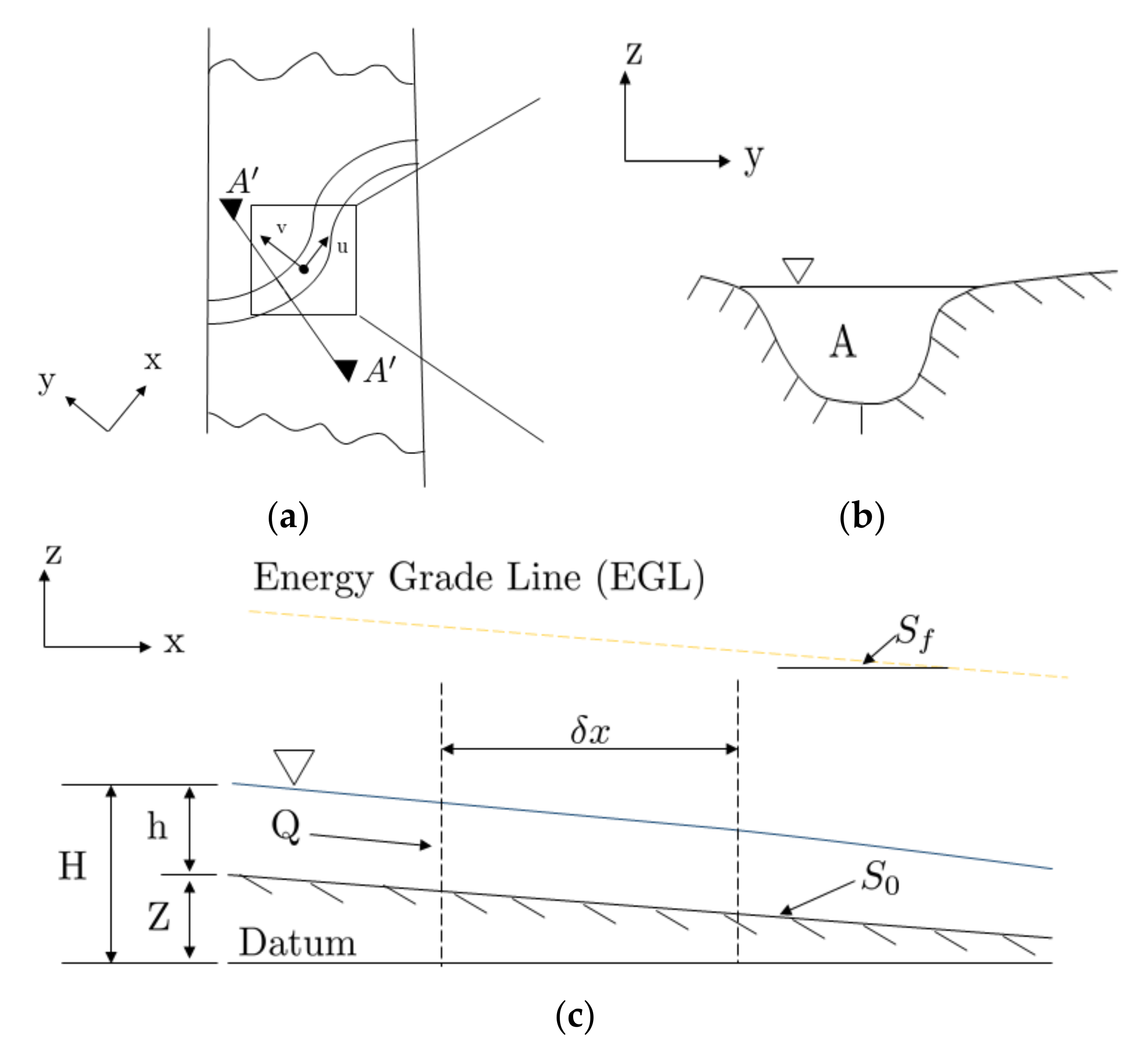
2.1. Governing Equations for 2D HEC-RAS Hydrodynamic Model

The HEC-RAS 2D model is developed to model and simulate complex floodplains in situations where the 1D flow is no longer valid enough for expected outcomes. The 2D unsteady flow varies with time and along two spatial dimensions. The governing laws of 2D unsteady flow are the conservation of mass (continuity) and conservation of momentum. The two-dimensional unsteady continuity equation is mathematically expressed in Equation (1).
H t + h u x + h v y = 0
where H is the water surface elevation (m), h is the water depth (m), u and v are the depth-averaged velocities in the x and y direction (m/s).
The conservation of momentum is calculated by Newton’s second law of motion, which states that the sum of forces acting on an element equals the rate of change of momentum, which is written by considering the gravitational force, eddy viscosity, friction, and Coriolis effect [29]. The Coriolis effect and the eddy viscosity terms are usually neglected in the 2D model due to the size of the river basin and to maintain uniformity in the comparisons with the 1D flow and the unavailability of the required parameters for the calibration of the eddy viscosity coefficient [30,31]. Therefore, the modified full momentum equations can be written as Equations (2) and (3) for x and y directions.
Momentum balance in x direction
u t + u u x + v u y + g H x + g   n 2 u R 4 / 3 u = 0
Momentum balance in y direction
v t + u v x + v v y + g H y + g   n 2 v R 4 / 3 v = 0
where g is the gravitational acceleration (m/s2), n is the Manning’s coefficient, and R is the wetted perimeter (m).
In order to reduce the computational time and the numerical instabilities, the HEC-RAS 2D unsteady flow Saint-Venant equations (shallow water equation) are often simplified using diffusive wave approximation. However, those simplifications are only valid for certain flow conditions. Nevertheless, the rivers that are influenced by tides are advised to incorporate the full momentum equations [31]. The Kelani River, which was used as an example in this study, has tidal influences [32,33] and, therefore, comprehensive analysis is recommended.

2.2. Governing Equations for 1D/2D HEC-RAS Hydrodynamic Model

The main river stretch is modelled as a 1D model, while the flood plain is a model with a 2D modelling approach in the coupled 1D/2D HEC-RAS model. The HEC-RAS uses a tight coupling technique. In other terms, both the 1D domain and the 2D domain are coupled on a time step basis. A lateral structure is used in order to establish the connection between the 1D and 2D domains [34].
The main river stretch solves the 1D Saint-Venant (shallow water) equation, which is comprised of continuity and momentum equations as shown in Equations (4) and (5).
A t + Q x = 0
t Q A + t Q 2 A 2 + g H x + g S 0 S f = 0
where, A ,   Q , S 0 , and S f are the cross section area (m2), the water flowrate (m3/s), the slope of the riverbed, and the energy slope, respectively. In addition, flow in the flood plain is calculated using 2D continuity equations and momentum equations as given in Equations (1)–(3).

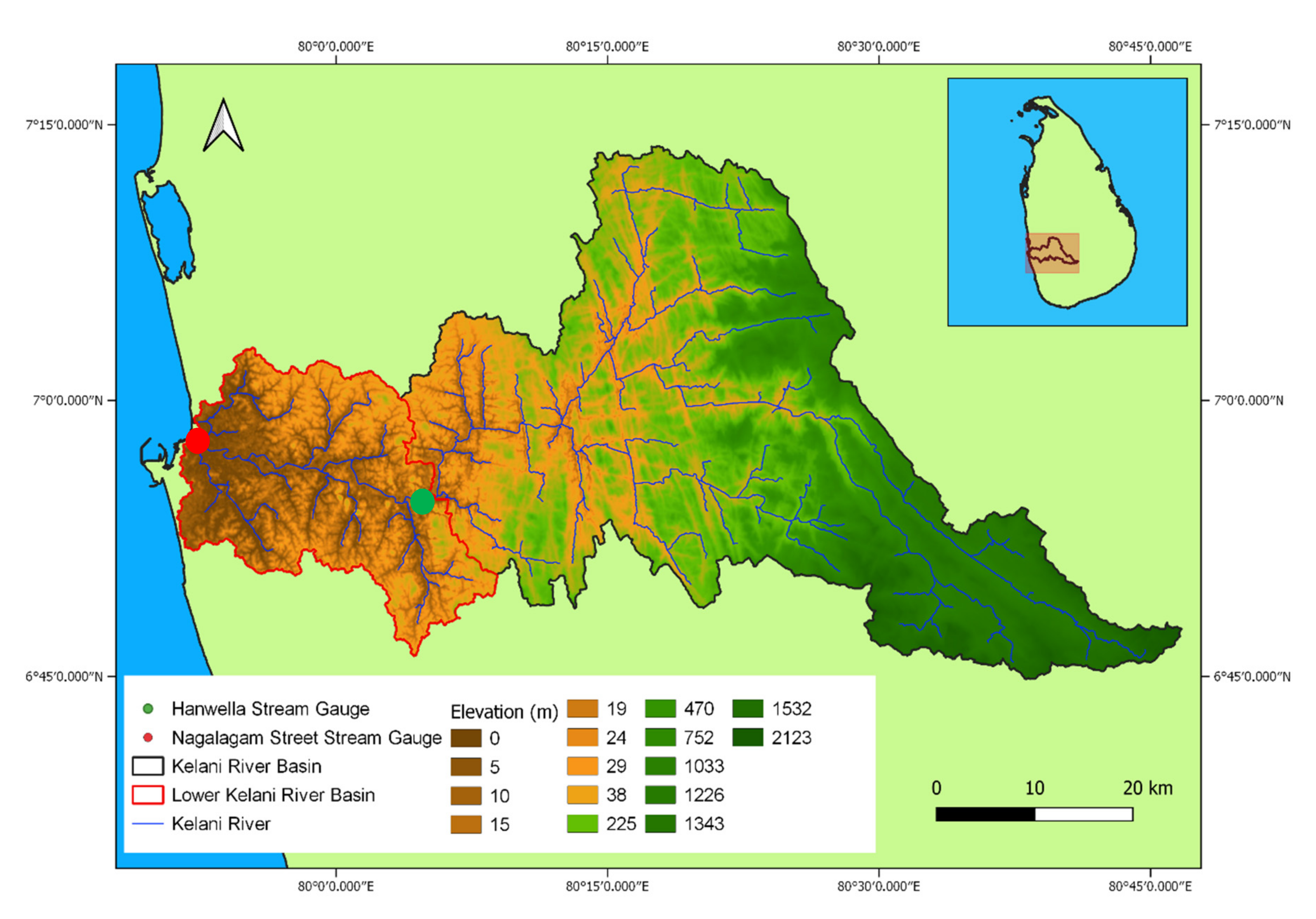
3. Case Study Application

The Kelani River basin in Sri Lanka is the second-largest river basin based on the catchment area. River Kelani extends from the central hills of the country to Colombo, at a distance of about 145 km when measured along the channel centreline. The river basin is located between Northern latitude 6°47′ to 7°05′ and Eastern longitudes 79°52′ to 80°13′, with a basin area of nearly 2230 km2 as shown in Figure 2. Broadly, the river basin can be categorized into upper and lower basins. The upper basin features mountainous terrain, whereas the lower basin is generally flat terrain. The lower basin lies below the Hanwella River gauging station, which has an approximate area of 500 km2 (refer to Figure 2, light brown area).
The upper catchment is predominantly covered with vegetation, whereas the lower catchment is heavily urbanized. The river basin receives an average annual rainfall of nearly 2400 mm and carries a peak discharge of 800–1500 m3/s during the monsoonal periods (i.e., especially in the southwest monsoon period from May to September). During the southwest monsoon period, the lower reach of the basin is frequently flooded as recorded from the flood gauge located at Nagalagam Street (refer to Figure 2).
Recurring flood events happened in consecutive years, 2016, 2017, and 2018, at the Lower Kelani River basin. Out of them, the 2016 event was recorded as the most severe flood in almost 30 years (compared to the flood that happened in 1989). Rapid urbanization, unplanned developments, and reduced drainage density were identified as the major causes for these flood events. According to (Sri Lanka post-disaster needs assessment: May 2016 floods and landslides, 2016) records, more than 60% of the total population in Colombo and Gampaha Districts were affected and significant damage to the infrastructure happened due to the 2016 event.

4. Methodology

4.1. Overall Methodology

It is interesting to observe the flood events under 1D and 2D hydraulic models and then to compare their capabilities. Therefore, Hydraulic Engineering Centre’s River System (HEC-RAS) was used to analyse the extreme events that happened in 2016 and 2018 using a combined one-dimensional and two-dimensional (1D/2D) model and two-dimensional (2D) model. In addition, a high-resolution Digital Elevation Model (DEM) was used to map the inundations during the flood events along the river and floodplains.

4.2. HEC-RAS Model Inputs

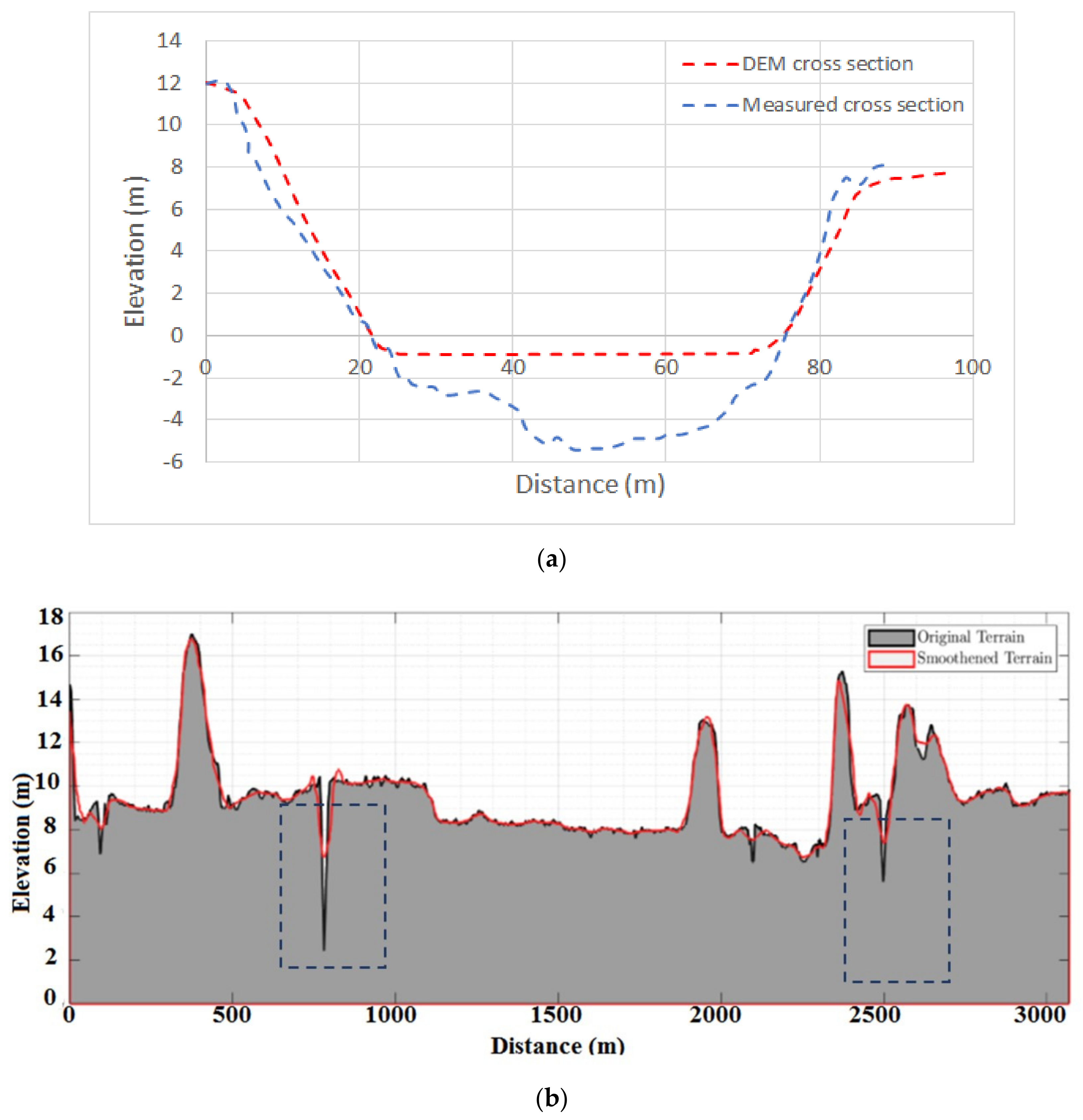
4.2.1. Elevation and Modification of River Bathymetry

The Digital Elevation Model (DEM) developed using Light Detection and Ranging (LiDAR) was used to capture the topographic features. However, the LiDAR data are unable to detect the terrain features underneath the water [35]. Figure 3a explains this feature. Therefore, measured bathymetries (river cross sections) were fed using a conventional manner. Perpendicular interpolations were conducted for the sections spaced approximately at a 1 km distance, which was also used by Nandalal [3]. These interpolations were important when the change in velocity head was too large to determine the energy gradient along the river. Furthermore, the inline structures (i.e., bridges and salinity barrier) were neglected when modelling the river stretch.
In developing the 1D/2D HEC-RAS model, the 2D area was connected to the main river stretch with lateral structures established next to the river over banks. A lateral structure has the same topographical features next to the river over banks. However, sudden variations in the elevation data can lead to model instabilities. As shown in Figure 3b, a smoothening was conducted to the elevations of the lateral structure by following “Savitzky–Golay” algorithm developed by Gorry [36]. However, some places were adjusted manually in order to have a good representation of the natural terrain (see Figure 3b).
The models were developed on a personal computer (HP—Elite Book i5) with an 8 core processor at a speed of 3.7 GHz and a RAM of 6 GB. The simulation times of 10 min and 45 s and 7 min and 32 s were taken for the combined 1D–2D model for 2016 and 2018, respectively. In addition, 17 min and 24 s and 6 min and 41 s were taken for the simulations of HEC-RAS 2D model for the 2016 and 2018 years, respectively.

4.2.2. Land Use Characteristics

The upper basin is predominantly covered with heavy vegetation such as forests, grasslands, scrublands, and cultivations, whereas the lower basin is heavily urbanized [37]. The preliminary manning’s coefficients were assigned based on the suggestions of Chow [38,39].

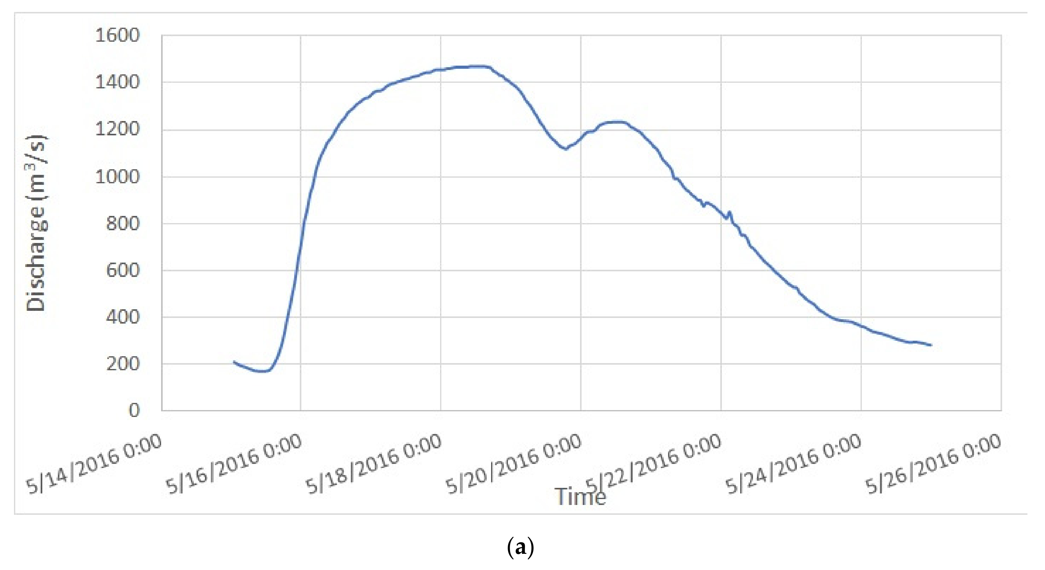
4.2.3. Boundary Conditions

An hourly flow hydrograph and a stage hydrograph were established as the upper and lower boundary conditions, respectively, for both models. These unsteady flow hydrographs are given in Figure 4 for years 2016 and 2018. Lower boundary conditions were established at the sea outfall by giving hourly tidal fluctuation (as stage). Therefore, the stage hydrograph at Nagalagam Street was able to replicate the tidal fluctuation including backwater effect [39]. Additionally, an energy slope for the distribution of flow along the boundary line was assigned after measuring an average slope from the DEM for the 2D model.

4.2.4. Implicit Weighting Factor, Calculation Time Step, and Optimal Mesh Size

As was already stated, the Kelani River is a tidally influenced river, and the bed elevation at the outfall is usually lower than the mean sea level. Therefore, the backwater effect has a significant impact on the flows. As the tidal fluctuations are very dynamic, Brunner [40] suggested maintaining an implicit weighting factor around 0.6 in order to have an accurate system. Therefore, a trial and error procedure was applied to identify the optimum value for theta weighting factor. The optimal weighting factor was identified as 0.71 for the Kelani River. The weighting factor is capable of performing stable calculation.
In addition, Courant number C was defined to ensure the model stability selection of time step and the mesh size. This Courant number is expressed in Equation 6.
C = u   Δ t Δ x < 1  
where   u is the flow velocity (m/s), Δ t is computational time step (s), and Δ x is the spatial step (m), i.e., cross section spacing in 1D models and cell size in 2D models. According to the Equation (6), the time step of 60 s was selected for the calculation. Minimum of 15 m fine cell resolution in the main channel and maximum of 30 m coarse cell resolution were used for the computational mesh for suitable locations of the river basin.

4.3. Model Analysis and Results Comparison

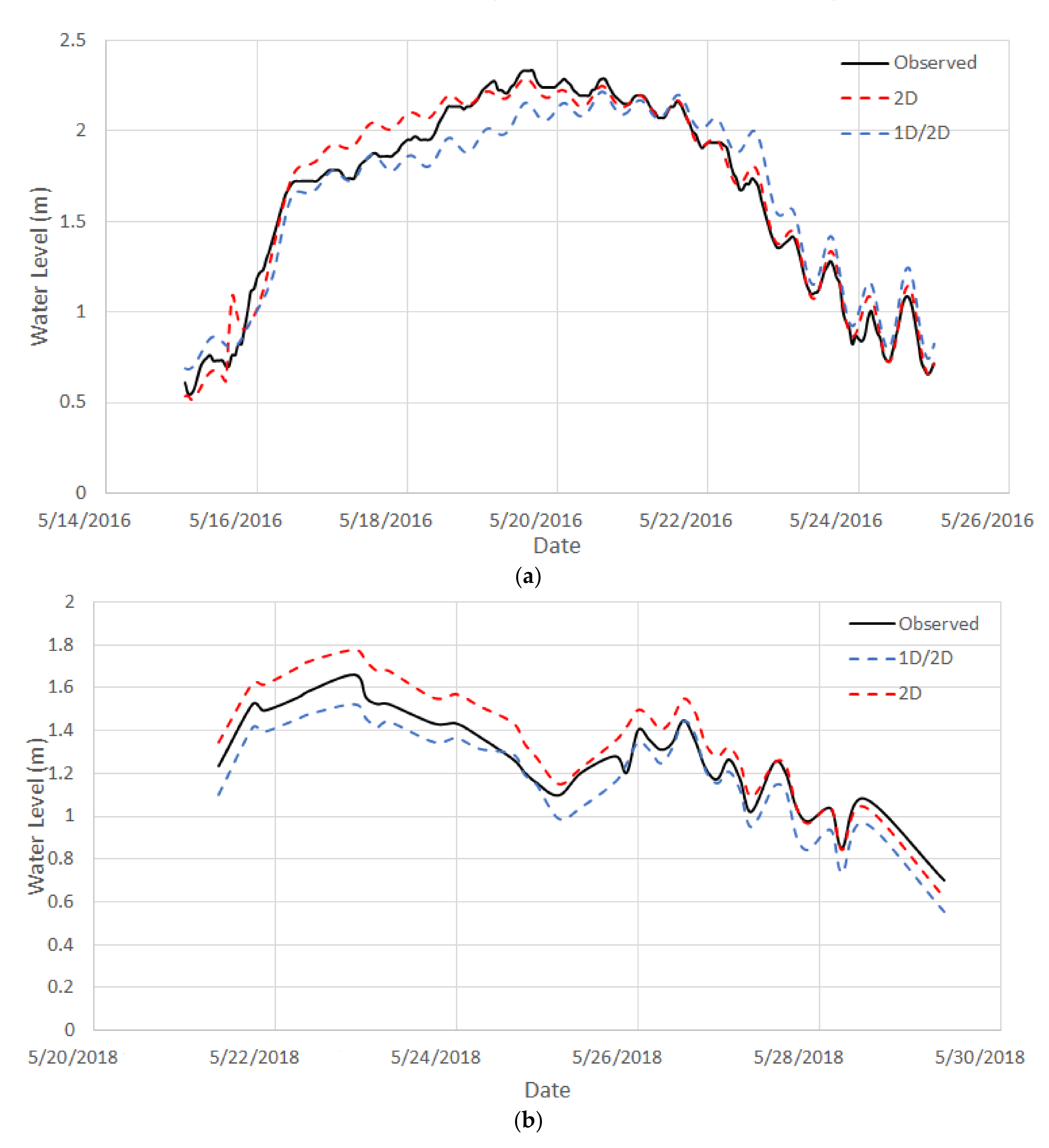
4.3.1. Water Level Comparison

The better agreement between the simulated water level in Nagalagam Street gauge and the observed water level was ensured with the use of the Nash–Sutcliffe efficiency coefficient (NSE) [41]. The value 1 in the Nash–Sutcliffe efficiency coefficient denotes a perfect match. Equation (7) presents the Nash–Sutcliffe efficiency coefficient.
N S E = 1 i = 1 n S i O i 2 i = 1 n O i O _ 2  
where O i is observed flow at ith time, S i is simulated flow at ith time, O _ is mean of observed flow, S _ is mean of simulated flow, and n is the number of observations.
In addition to this, Pearson coefficient of determination (R2) and Root Mean Square Error (RMSE) were calculated to ensure a good capture of the correlation and minimize the error between simulated and observed water levels. These are given in Equations (8) and (9).
R 2 = i = 1 n O i O _ × S i S _ 2 i = 1 n O i O _ 2 × S i S _ 2
R M S E = 1 n i = 1 n O i S i 2

4.3.2. Inundation Extent Comparison

A comprehensive evaluation with satellite-observed inundation extents and surveyed inundations were carried out to evaluate the model’s performance. Flood Area Index ( F A I ), accuracy, Bias score, Probability of Detection, false alarm ratio, Probability of False Detection, and Success Index were extracted from Bennett et al. [42], Falter et al. [43], and Khaing et al. [44] in order to compare the inundation extents. A self-explanatory skill matrix composed of Equations (10)–(16) was developed.
F A I = M 1 D 1 M 1 D 1 + M 1 D 0 + M 0 D 1  
A c c u r a c y = h i t s + c o r r e c t   n e g a t i v e s t o t a l  
B i a s   s c o r e = h i t s + f a l s e   a l a r m s h i t s + m i s s e s  
P r o b a b i l i t y   o f   D e t e c t i o n   h i t   r a t e = h i t s h i t s + m i s s e s  
F a l s e   a l a r m   r a t i o = f a l s e   a l a r m s h i t s + f a l s e   a l a r m s  
P r o b a b i l i t y   o f   F a l s e   D e t e c t i o n   f a l s e   a l a r m   r a t e = f a l s e   a l a r m s c o r r e c t   n e g a t i v e s + f a l s e   a l a r m s  
S u c c e s s   I n d e x = 1 2   h i t s h i t s + m i s s e s + c o r r e c t   n e g a t i v e s   c o r r e c t   n e g a t i v e s + f a l s e   a l a r m s  
where M 1 D 1 is the number of grid cells correctly predicted as flooded by the model (hits), M 1 D 0   is the number of cells flooded in the prediction but observed as dry in the observation (false alarm), M 0 D 1   is the predicted dry area but observed wet area (misses), and the number of correct negatives are the cells predicted and observed as dry.

4.3.3. Calibration and Validation

The calibration of the hydrodynamic model was conducted by following a trial and error procedure while changing Manning’s coefficients. The initial guesses for Manning’s roughness coefficients were assigned based on the land use type along with visual observations. Suggestions of Chow (1959) were further used for the justification of the values applied for the model.

5. Results and Discussion

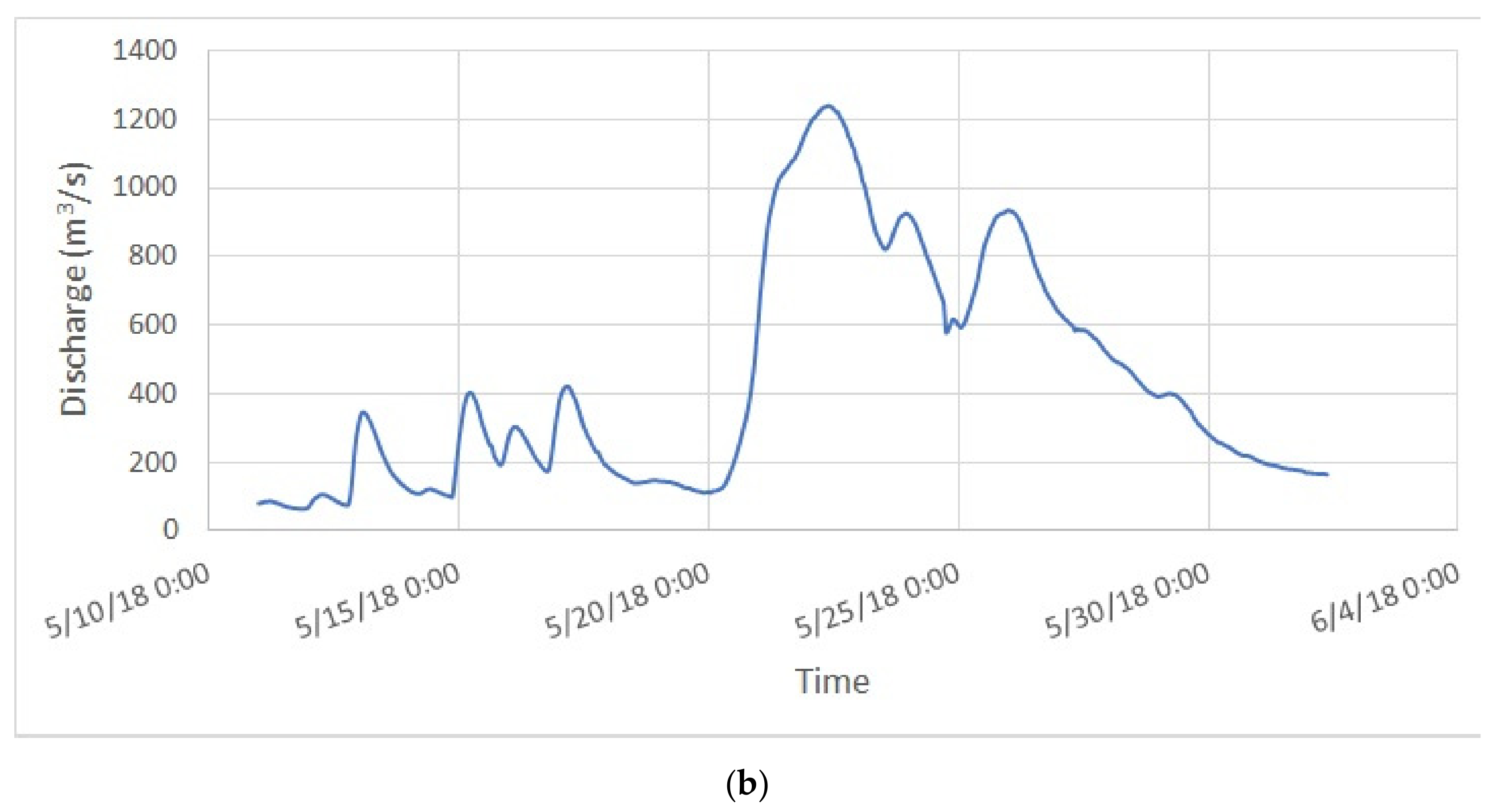
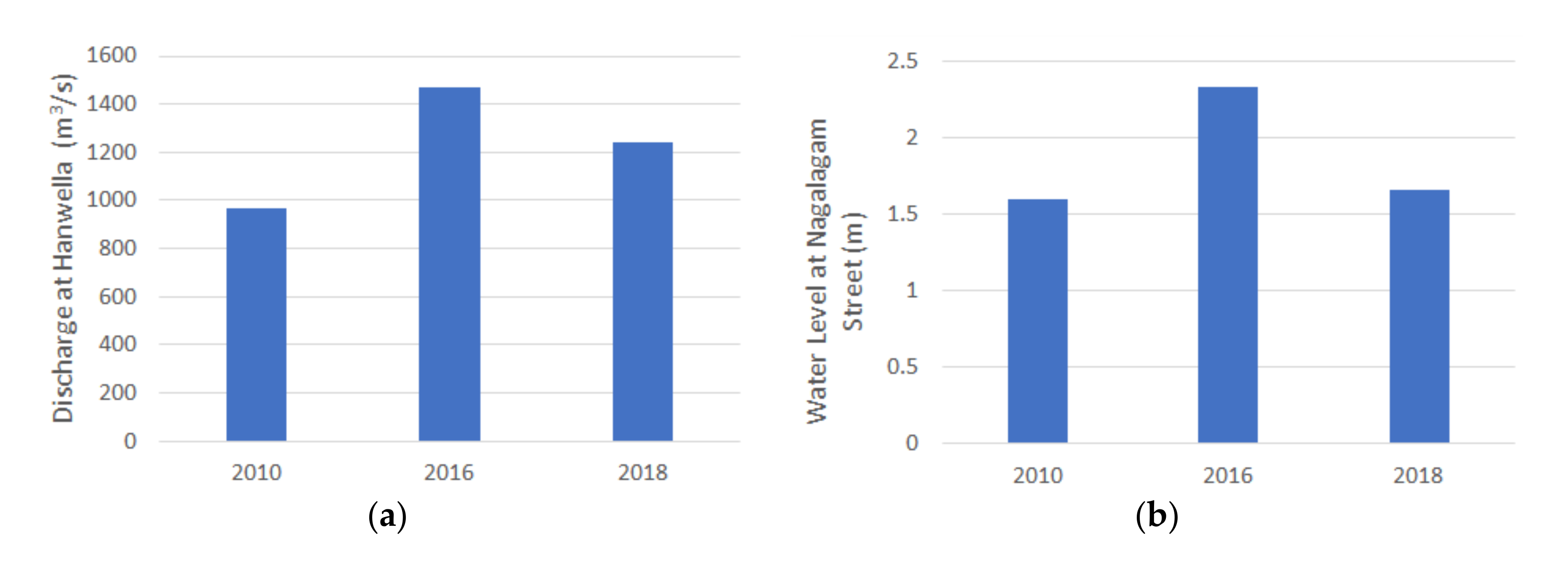
5.1. Comparison of 2016 and 2018 Flood Stages

The year 2016 flood was an extreme event and the stages recorded at Nagalagam Street was observed to be almost at 2.4 m, which was the highest recorded flood after 1989. Figure 5a showcases the stage heights comparison from the observed to simulated stages, while Figure 5b presents those in 2018. Usually, the 2D model overestimated the flood heights compared to the observed heights. However, on average, slight underestimations can be seen in the results of the 1D/2D model. Nevertheless, the 2D hydraulic model can be considered a better model by the visual observations from Figure 5a,b.
The time to the peak is also well captured by the 2D model compared to the 1D/2D model. Nevertheless, overestimations, as discussed earlier, can be observed in the 2D model. The performance of the 1D/2D and 2D models with respect to the stages for years 2016 and 2018 were evaluated with statistical parameters suggested by Moriasi et al. [45], as stated in the methodology section. The calculated statistical parameters comparing the simulated stages with the observed stages are given in Table 1. Based on the calculated statistical parameters, the overall model is capable of capturing the flow processes with both models showing a very good performance rating.
According to the estimated statistical parameters for both the 1D/2D and 2D models, the 2D model shows a high prediction capability of stages (i.e., NSE = 0.98, R2 = 0.98, and RMSE = 0.08) compared to the 1D/2D model (i.e., NSE = 0.95, R2 = 0.91, and RMSE = 0.14). However, the 1D/2D model was comparatively able to capture the flow processes better than the 2D model for the 2018 event. Nevertheless, by comparing the visual characteristics of the hydrograph and the statistical parameters, it can be stated that the 2D model outperforms the 1D/2D model.

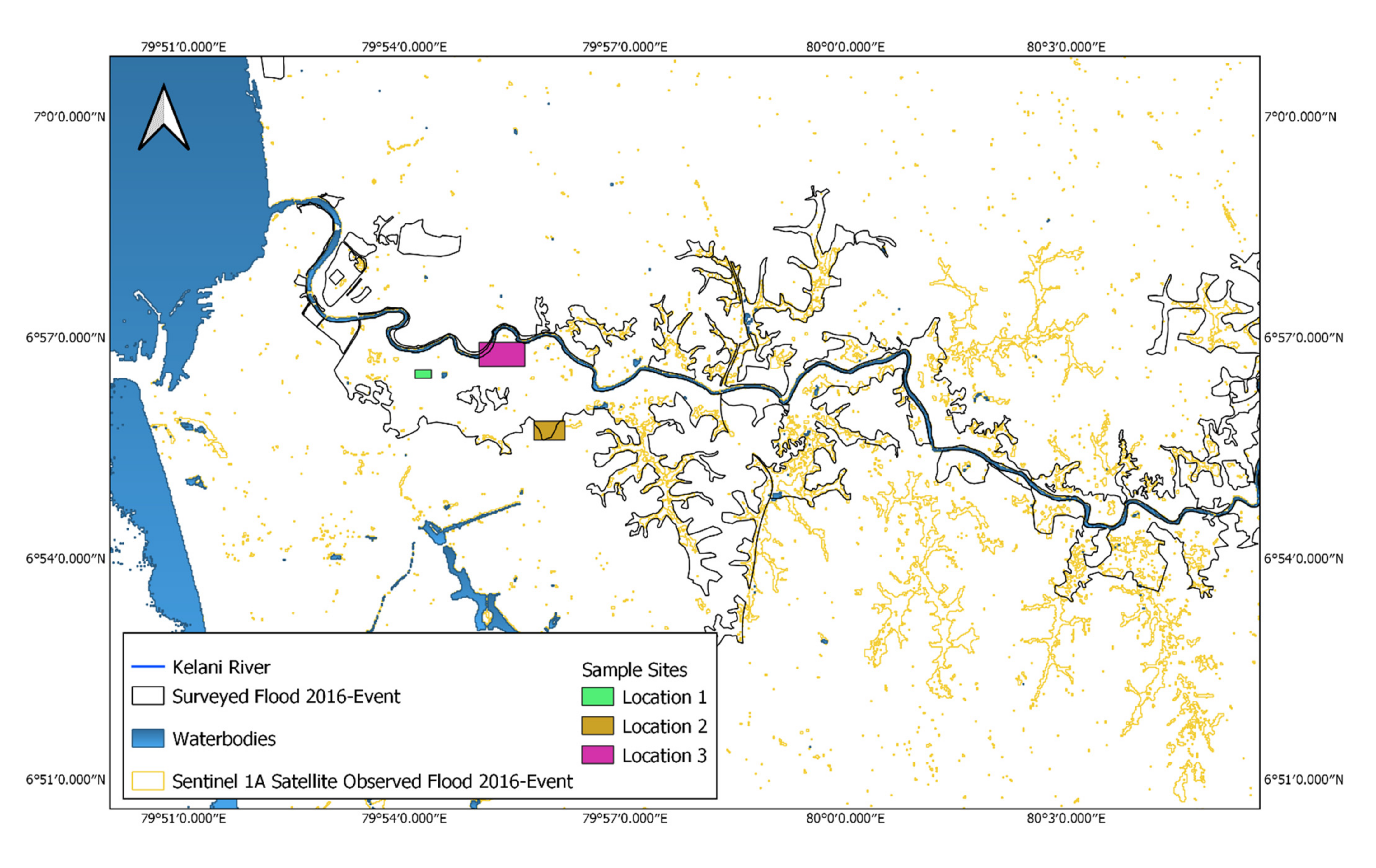
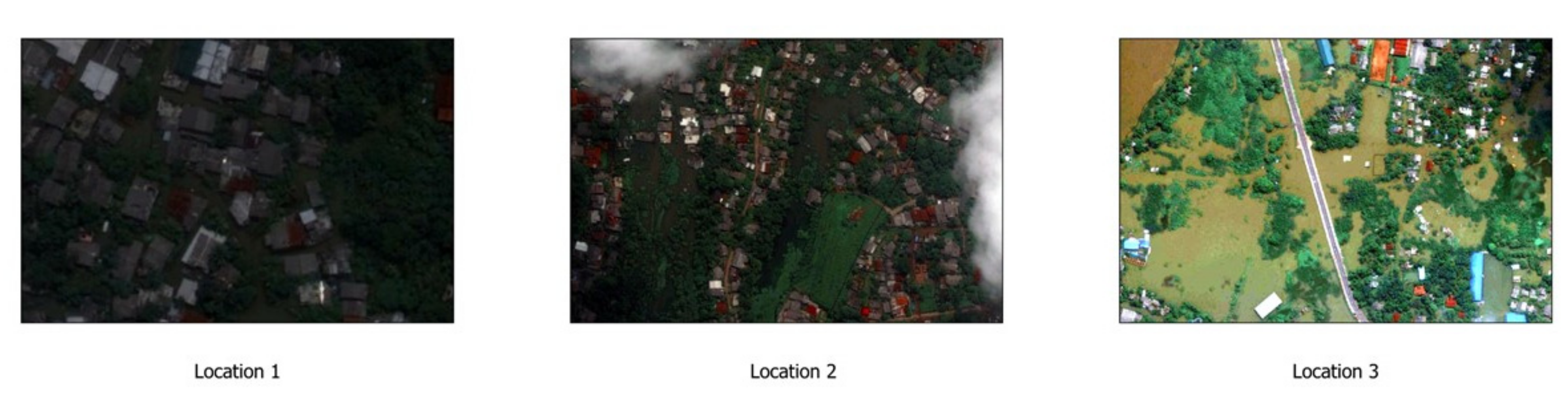
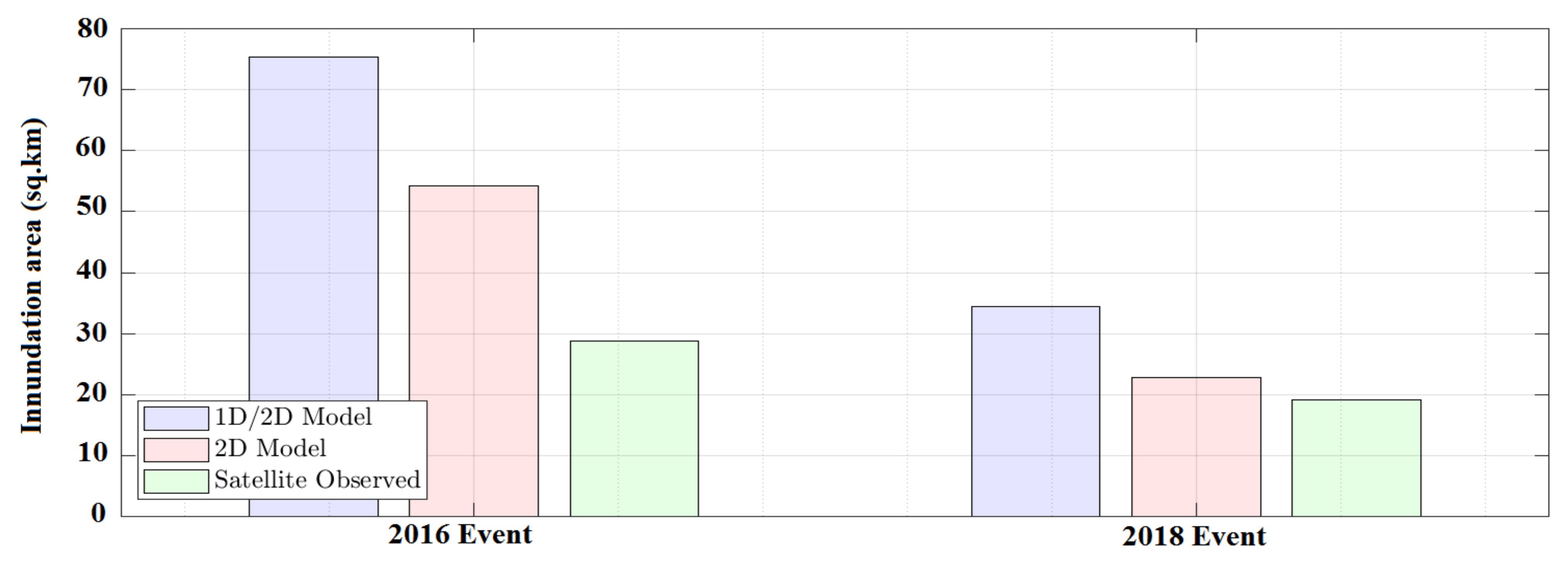
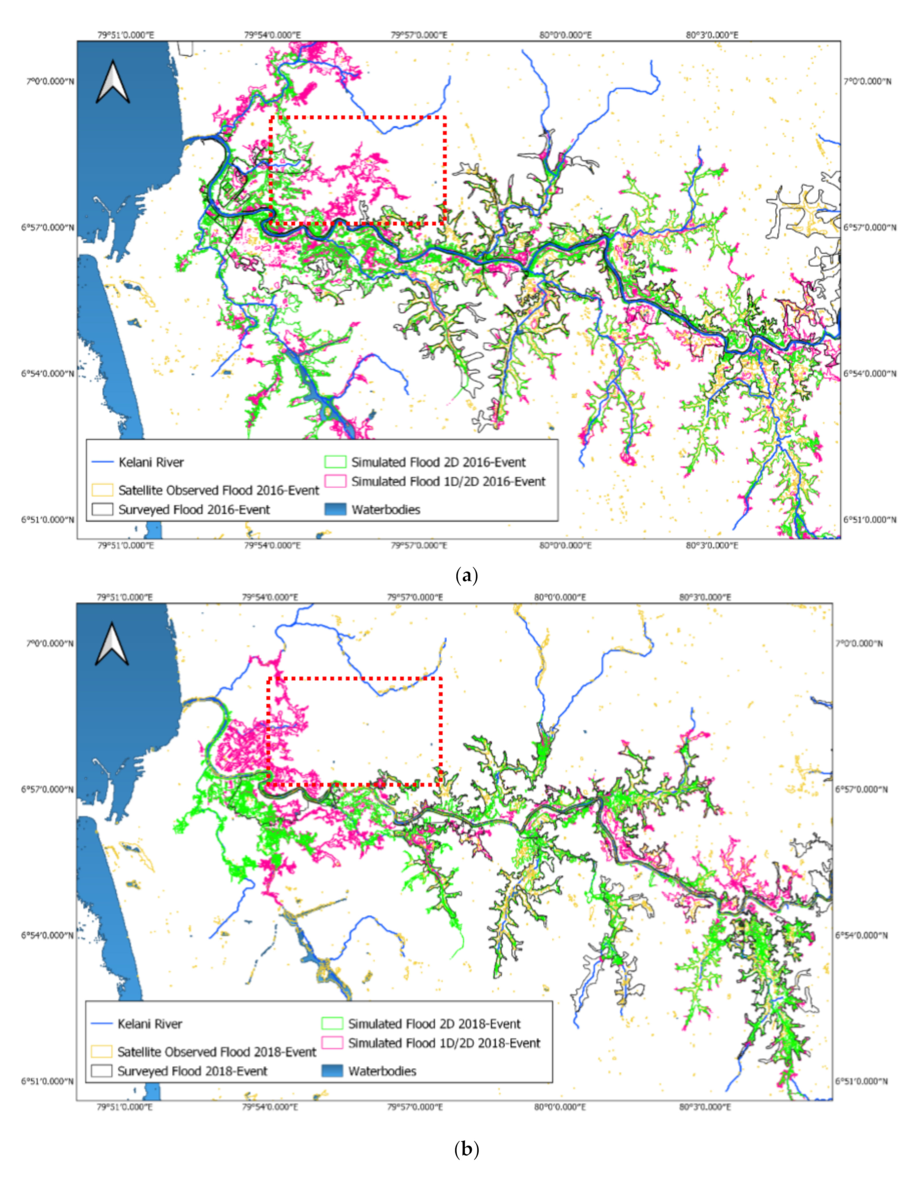
5.2. Inundation Extent Comparison

The microwave images captured by Sentinel-1 during the floods of 2016 and 2018 were processed and used to compare the simulated inundation extent. The comparisons were conducted by following a cell by cell approach of sub-regions suggested by De Silva et al. [46] and evaluated with the statistical parameters mentioned above. However, the inundation extents of some areas, especially the highly urbanized and mountainous areas, are partly constricted by the satellite images [43]. Figure 6 shows a comparison between the surveyed inundations with the Sentinel-1 satellite-observed inundation extent.
Locations 1–3 were areas that actually experienced floods during the 2016 event, which are marked with the surveyed inundation and further justified with Google Earth pro high-resolution images. However, these were not captured by the Sentinel-1 satellite image. The incoming signals of Sentinel-1 could have been double bounced, causing the backscatter to be higher than normal due to the densely built-up areas and, therefore, the signal was unable to reach the ground. This scenario was stated by Solbø and Solheim [47]. This could be a possible reason for not capturing the three locations. Therefore, there can be some underestimations of flood cover in satellite images, even though they are considered one of the most reliable sources to make comparisons with the simulated extent [43].
Figure 7 illustrates the inundated areas from the 2016 and 2018 floods for the river basin using satellite observations and hydrological models (1D/2D and 2D).
Based on the derived inundation maps for the 2016 and 2018 events, the predicted inundation areas from the 1D/2D model were 75.24 km2 and 34.47 km2 for the 2016 and 2018 floods, respectively, whereas the predicted inundation areas from the 2D model were 54.19 km2 and 22.86 km2, respectively. Therefore, the 1D/2D model predicts more inundation area compared to the 2D model. Moreover, the inundated areas calculated from the Sentinel-1 satellite images are lower than the inundation extents simulated from both models. These are approximately 14.28 km2 and 3.51 km2, respectively. Most of the flooded areas in the Colombo and Gampaha districts were not captured by the satellite images. However, high-resolution satellite images of Google Earth Engine (refer to Figure 6) showcase the flooded areas that were not captured by the Sentinel-1 satellite images.
Furthermore, Figure 8a,b present the simulated inundation areas for both models for the 2016 and 2018 flood events along with the satellite-observed inundation extent and the recorded surveyed inundation for urban areas.
The inundated area observed during the 2016 flood event is comparatively larger than in 2018, as it was an extreme event. Apparently, both models have many overlapping areas. In order to have a comprehensive assessment, sub-region-based cell by cell comparison was conducted for both models with the satellite-observed flood, which is summarised in Table 2.
For the event in 2016, the 1D/2D model showed a very good agreement with the satellite-observed flood, which is indicated with a probability of detection (hit rate) of 97% and an accuracy of 88%. However, the model tends to overestimate the inundation extent, which can be identified by the false alarm ratio of 48%, a false alarm rate of 13%, and a biased score of 1.97. Nevertheless, the 1D/2D model was able to successfully predict the inundation extent with a success index of 92% for the 2016 event. This is a significantly improved result when compared to past studies for the same basin [42,46].
However, the 2D model was unable to predict the extent as it was in the 1D/2D model for 2016, which is illustrated with a hit rate of 68% and an accuracy of 86%. Furthermore, a similar overestimation was observed when compared to the 1D/2D model, which is quantified with a false alarm ratio of 50%, a false alarm rate of 12%, and a biased score of 1.49. Due to that, the occurrence or non-occurrence of the event was captured with a 78% success index. Therefore, the 2D model for the 2016 event was able to reasonably capture the inundation extent.
However, the 1D/2D model predictions showed a slightly better performance for the 2018 event compared to the 2016 flood event, which is denoted by an increased accuracy of 94%, a reduced bias score (1.35), a lower false alarm ratio (34%), and a lower false alarm rate (5%), but it has a lower hit rate (83%). As a result, the prediction ends up with a success index of 89%, slightly lower when compared to the 2016 event.
The 2D model for the 2018 event showcases similar behaviour as was shown for the 2016 event. It indicated a hit rate of 41%, an accuracy of 89%, a false alarm ratio of 50%, and a false alarm rate of 6%. However, the 2D model underestimates the inundation extent, which is denoted with a bias score of 0.99. Therefore, the success index of the 2D model for the year 2018 is 73%.
After combining the results for both events, the 1D/2D model was able to successfully predict the inundation extent with a high hit rate (90%) and a high accuracy (91%), together with an overestimation denoted by statistical parameters such as false alarm ratio (41%), false alarm rate (9%), and biased score (1.66). Based on the statistical results, the 2D model was unable to predict the inundations in the same way as the 1D/2D model. Even the predictions showed an underestimation when compared with satellite-observed inundation extents.
Even the statistical matrix showed a good agreement: in visual observations, the combined 1D/2D model (refer to Figure 8a,b—pink outline highlighted with red coloured dotted box) seems to be an overestimation. However, during the flood events, those areas were inundated. However, there was no valid proof in the scientific world other than the statements of local people. Therefore, to justify the statement, “during the flood events, those areas were inundated”, we conducted a comparison with the recorded maximum discharges at Hanwella Gauge, and the stages at Nagalagam Street with past studies conducted by the Disaster Management Centre Sri Lanka (DMC) and the University of Kelaniya, Sri Lanka [48].
The initial environmental examination conducted by the University of Kelaniya [48] showed some photographs captured during the 2010 flood and the recorded flood surface elevation (2.10 m above MSL), which justify that the area was inundated with the maximum recorded discharge of 907.8 m3/s at Hanwella gauge and a stage of 1.58 m at Nagalagam Street gauge (refer to Figure 9).
However, the recorded flood events in 2016 (1470 m3/s) and 2018 (1238 m3/s) had higher magnitudes compared to 2010 (964 m3/s). Based on that judgement, the statement can be justified. Therefore, the predicted flood inundations in the 1D/2D model are acceptable.

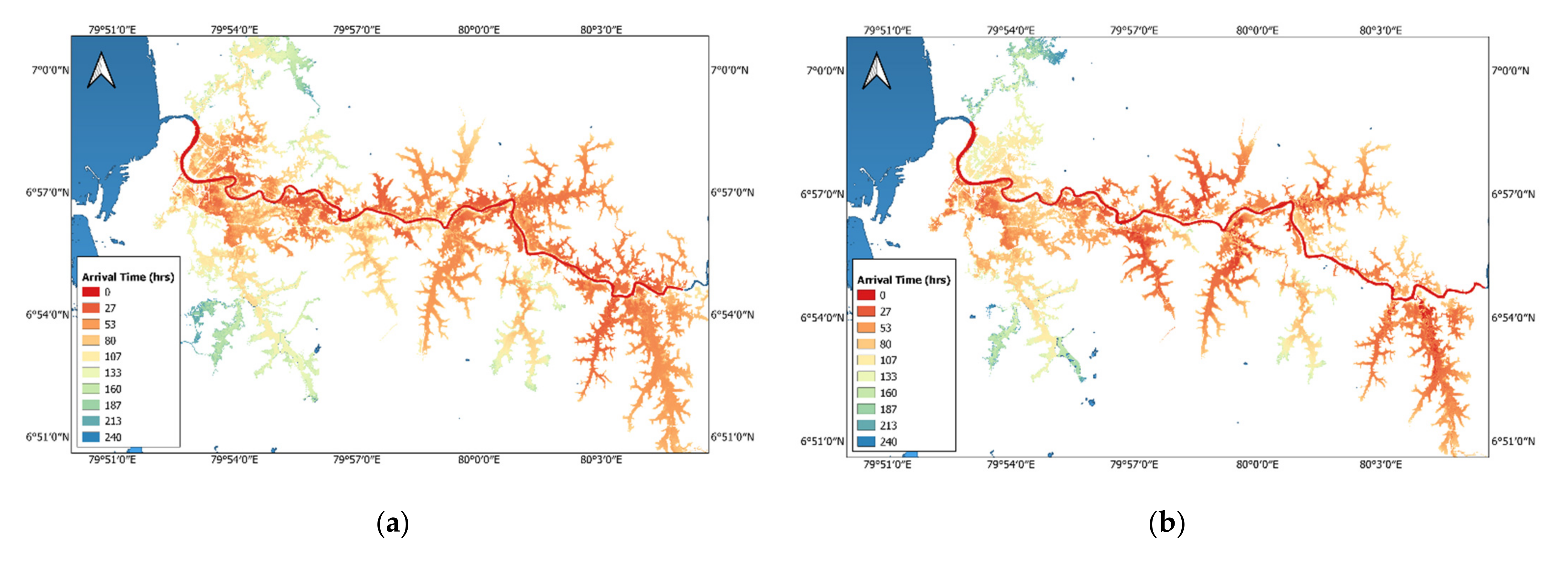
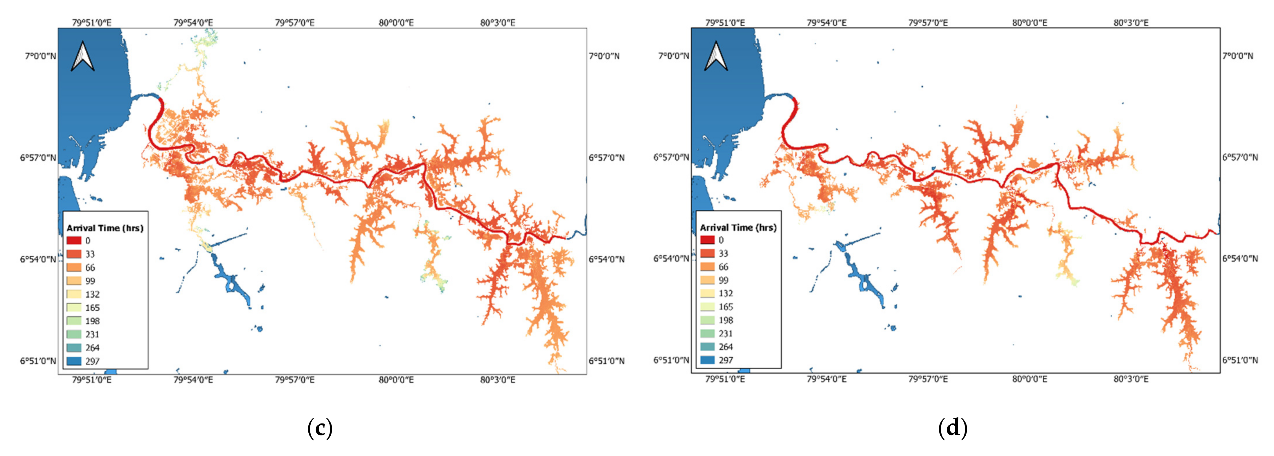
5.3. Travel Time Comparison

Figure 10 showcases the travel time comparison for both the 1D/2D and 2D models for both flood events (2016 and 2018). The spatial distribution of the flood arrival time was calculated. Both models were solved using the same 2D equation in the floodplain and, therefore, the travel time was similar. However, the mean travel time for most of the areas either side of the river bank was approximately 1 day (24 h) from the beginning of the flood wave.

6. Summary and Conclusions

The present study was conducted with high-resolution spatial data by two hydraulic models, which are solved in the 1D and 2D environments (1D/2D model and 2D model). The comparisons are conducted with coupled 1D/2D and 2D models of HEC-RAS, which has not been comprehensively studied in terms of capturing the inundations with the flows in the Sri Lankan context. Therefore, the major objective of comparing both models was conducted without changing the topography, channel geometries, boundary conditions, flows, and stages. The calibration was conducted by changing Manning’s coefficient and validated for similar flood scenarios that happened closer to the calibrated event. Based on the comparisons conducted, the following conclusions were made.
  • The HEC-RAS 2D model was able to successfully capture the flow process when compared to the coupled 1D/2D HEC-RAS models during high flow conditions.
  • The 1D/2D HEC-RAS model was a better predictor of flows when it came to low flow situations.
  • Combining the prediction capability of flows during high flows and low flows, the HEC-RAS 1D/2D model is a better predictor than the 2D model.
  • The HEC-RAS coupled 1D/2D model is a better predictor when predicting inundation extents during high flow and low flow situations.
  • Overall, the HEC-RAS 1D/2D model is a better model compared to the 2D model in predicting inundation extents and the flows under high and low flow situations.
The results would be interesting to the stakeholders such as the Disaster Management Centre of Sri Lanka to forecast the future needs based on the capacity of the hydraulic model.

Author Contributions

Conceptualization, J.T.S. and U.R.; methodology, J.T.S. and V.B.; software, J.T.S. and V.B.; validation, J.T.S. and V.B.; formal analysis, J.T.S. and V.B.; writing—original draft preparation, J.T.S.; writing—review and editing, M.B.G., H.M.A. and U.R.; supervision, U.R.; funding acquisition, U.R. All authors have read and agreed to the published version of the manuscript.

Funding

This research was carried out under the Sri Lanka Institute of Information Technology; SLIIT Research Grant of FGSR/RG/FE/2021/11.

Data Availability Statement

Data used in this research can be requested from the corresponding author for research purposes.

Acknowledgments

Authors would like to acknowledge the support received from the Sri Lanka Institute of Information Technology (SLIIT), Sri Lanka to carry out this research work.

Conflicts of Interest

The authors declare no conflict of interest.

References

  1. UNISDR. The Human Costs of Weather-Related Disasters. 2015. Available online: https://www.unisdr.org/2015/docs/climatechange/COP21_WeatherDisastersReport_2015_FINAL.pdf (accessed on 30 December 2021).
  2. Caddis, B.; Nielsen, C.; Hong, W.; Tahir, P.A.; Teo, F.Y. Guidelines for floodplain development—A Malaysian case study. Int. J. River Basin Manag. 2012, 10, 161–170. [Google Scholar] [CrossRef]
  3. Nandalal, K. Use of a hydrodynamic model to forecast floods of Kalu River in Sri Lanka. J. Flood Risk Manag. 2009, 2, 151–158. [Google Scholar] [CrossRef]
  4. Apel, H.; Thieken, A.; Merz, B.; Bloschl, G. Flood risk assessment and associated uncertainty. Nat. Hazards Earth Syst. Sci. 2004, 4, 295–308. [Google Scholar] [CrossRef]
  5. Morris, M.; Hassan, M.; Vaskinn, K. Breach formation: Field test and laboratory experiments. J. Hydraul. Res. 2007, 45 (Suppl. 1), 9–17. [Google Scholar] [CrossRef]
  6. Thieken, A.H.; Kienzler, S.; Kreibich, H.; Kuhlicke, C.; Kunz, M.; Mühr, B.; Müller, M.; Otto, A.; Petrow, T.; Pisi, S.; et al. Review of the flood risk management system in Germany after the major flood in 2013. Ecol. Soc. 2016, 21, 51. [Google Scholar] [CrossRef]
  7. Vorogushyn, S.; Lindenschmidt, K.-E.; Kreibich, H.; Apel, H.; Merz, B. Analysis of a detention basin impact on dike failure probabilities and flood risk for a channel-dike-floodplain system along the river Elbe, Germany. J. Hydrol. 2012, 436–437, 120–131. [Google Scholar] [CrossRef] [Green Version]
  8. Barredo, J.I.; Sauri, D.; Llasat, M.C. Assessing trends in insured losses from floods in Spain 1971–2008. Nat. Hazards Earth Syst. Sci. 2012, 12, 1723–1729. [Google Scholar] [CrossRef] [Green Version]
  9. Cunderlik, J.M.; Ouarda, T.B. Trends in the timing and magnitude of floods in Canada. J. Hydrol. 2009, 375, 471–480. [Google Scholar] [CrossRef]
  10. Kundzewicz, Z.W.; Pińskwar, I.; Brakenridge, G.R. Large floods in Europe, 1985–2009. Hydrol. Sci. J. 2013, 58, 1–7. [Google Scholar] [CrossRef]
  11. Najibi, N.; Devineni, N. Recent trends in the frequency and duration of global floods. Earth Syst. Dyn. 2018, 9, 757–783. [Google Scholar] [CrossRef] [Green Version]
  12. Baker, J.L. Climate Change, Disaster Risk, and the Urban Poor: Cities Building Resilience for a Changing World; The World Bank: Washington, DC, USA, 2012. [Google Scholar]
  13. Egbinola, C.; Olaniran, H.; Amanambu, A. Flood management in cities of developing countries: The example of Ibadan, Nigeria. J. Flood Risk Manag. 2017, 10, 546–554. [Google Scholar] [CrossRef]
  14. Teo, F.Y.; Falconer, R.A.; Lin, B.; Xia, J. Investigations of hazard risks relating to vehicles moving in flood. J. Water Resour. Manag. 2012, 1, 52–66. [Google Scholar]
  15. Teo, F.Y.; Xia, J.; Falconer, R.A.; Lin, B. Experimental studies on the interaction between vehicles and floodplain flows. Int. J. River Basin Manag. 2012, 10, 149–160. [Google Scholar] [CrossRef]
  16. Daksiya, V.; Mandapaka, P.V.; Lo, E.Y.M. Effect of climate change and urbanisation on flood protection decision-making. J. Flood Risk Manag. 2020, 14, e12681. [Google Scholar] [CrossRef]
  17. Kay, A.; Rudd, A.; Fry, M.; Nash, G.; Allen, S. Climate change impacts on peak river flows: Combining national-scale hydrological modelling and probabilistic projections. Clim. Risk Manag. 2021, 31, 100263. [Google Scholar] [CrossRef]
  18. Mehryar, S.; Surminski, S. National laws for enhancing flood resilience in the context of climate change: Potential and shortcomings. Clim. Policy 2021, 21, 133–151. [Google Scholar] [CrossRef]
  19. Ponting, J.; Kelly, T.J.; Verhoef, A.; Watts, M.; Sizmur, T. The impact of increased flooding occurrence on the mobility of potentially toxic elements in floodplain soil—A review. Sci. Total Environ. 2021, 754, 142040. [Google Scholar] [CrossRef]
  20. Lea, D.; Yeonsu, K.; Hyunuk, A. Case study of HEC-RAS 1D–2D coupling simulation: 2002 Baeksan flood event in Korea. Water 2019, 11, 2048. [Google Scholar]
  21. Vozinaki, A.-E.K.; Morianou, G.G.; Alexakis, D.D.; Tsanis, I.K. Comparing 1D and combined 1D/2D hydraulic simulations using high-resolution topographic data: A case study of the Koiliaris basin, Greece. Hydrol. Sci. J. 2016, 62, 642–656. [Google Scholar] [CrossRef]
  22. Betsholtz, A.N.B. Potentials and Limitations of 1D, 2D and Coupled 1D-2D Flood Modelling in HEC-RAS. Master’s Thesis, Lund University, Lund, Sweden, 2017; pp. 1–128, Report number TVVR17/5003. [Google Scholar]
  23. Cook, A.; Merwade, V. Effect of topographic data, geometric configuration and modeling approach on flood inundation mapping. J. Hydrol. 2009, 377, 131–142. [Google Scholar] [CrossRef]
  24. Horritt, M.; Bates, P. Evaluation of 1D and 2D numerical models for predicting river flood inundation. J. Hydrol. 2002, 268, 87–99. [Google Scholar] [CrossRef]
  25. Timbadiya, P.V.; Patel, P.L.; Porey, P.D. Calibration of HEC-RAS model on prediction of flood for lower Tapi River, India. J. Water Resour. Prot. 2011, 3, 805–811. [Google Scholar] [CrossRef] [Green Version]
  26. Jun, S.M.; Song, J.-H.; Choi, S.-K.; Lee, K.-D.; Kang, M.S. Combined 1D/2D Inundation Simulation of Riverside Farmland using HEC-RAS. J. Korean Soc. Agric. Eng. 2018, 60, 135–147. [Google Scholar] [CrossRef]
  27. Patel, D.P.; Ramirez, J.A.; Srivastava, P.K.; Bray, M.; Han, D. Assessment of flood inundation mapping of Surat city by coupled 1D/2D hydrodynamic modeling: A case application of the new HEC-RAS 5. Nat. Hazards 2017, 89, 93–130. [Google Scholar] [CrossRef]
  28. Pasquier, U.; He, Y.; Hooton, S.; Goulden, M.; Hiscock, K.M. An integrated 1D–2D hydraulic modelling approach to assess the sensitivity of a coastal region to compound flooding hazard under climate change. Nat. Hazards 2018, 98, 915–937. [Google Scholar] [CrossRef] [Green Version]
  29. Brunner, G. HEC—RAS, River Analysis System Hydraulic Reference Manual; US Army Corps Engineers, Hydrologic Engineering Center: Davis, CA, USA, 2016. [Google Scholar]
  30. Brunner, G. HEC-RAS 5.0 2D Modeling User’s Manual; US Army Corps Engineers, Hydrologic Engineering Center: Davis, CA, USA, 2016. [Google Scholar]
  31. Raman, A.; Liu, F. An investigation of the Brumadinho Dam Break with HEC RAS simulation. arXiv 2019, arXiv:1911.05219. [Google Scholar]
  32. Gunathilaka, M.; Wikramanayake, W.; Perera, D.; Lanka, S. Identifying the impact of tidal level variation on river basin flooding. In Proceedings of the National Conference on Water, Food Security, and Climate Change in Sri Lanka, BMICH, Colombo, Sri Lanka, 9–11 June 2009; Water Quality, Environment, and Climate Change. IWMI: Colombo, Sri Lanka, 2010; Volume 2, p. 119. [Google Scholar]
  33. Hettiarachchi, P. Hydrological Report on the Kelani River Flood in May 2016; Department of Irrigation: Colombo, Sri Lanka, 2020. [Google Scholar]
  34. Brunner, G. Combined 1D and 2D Modelling with HEC–RAS, v. 5; US Army Corps Engineers, Hydrologic Engineering Center: Davis, CA, USA, 2016. [Google Scholar]
  35. Podhorányi, M.; Fedorcak, D. Inaccuracy introduced by LiDAR-generated cross sections and its impact on 1D hydrodynamic simulations. Environ. Earth Sci. 2015, 73, 1–11. [Google Scholar] [CrossRef]
  36. Gorry, P.A. General least-squares smoothing and differentiation by the convolution (Savitzky-Golay) method. Anal. Chem. 1990, 62, 570–573. [Google Scholar] [CrossRef]
  37. De Silva, M.M.G.T.; Weerakoon, S.B.; Herath, S. Modeling of event and continuous flow hydrographs with HEC–HMS: Case study in the Kelani River Basin, Sri Lanka. J. Hydrol. Eng. 2014, 19, 800–806. [Google Scholar] [CrossRef]
  38. Chow, V.T. Open-Channel Hydraulics; McGraw-Hill Civil Engineering Series; Kogakusha Company LTD: Tokyo, Japan; McGraw-Hill Publishers: New York, NY, USA, 1959. [Google Scholar]
  39. Bakhtyar, R.; Maitaria, K.; Velissariou, P.; Trimble, B.; Mashriqui, H.; Moghimi, S.; Abdolali, A.; Van Der Westhuysen, A.J.; Ma, Z.; Clark, E.P.; et al. A New 1D/2D coupled modeling approach for a riverine-estuarine system under storm events: Application to Delaware River Basin. J. Geophys. Res. Oceans 2020, 125, e2019JC015822. [Google Scholar] [CrossRef]
  40. Brunner, G. HEC—RAS River Analysis System User’s Manual Version 5.0; US Army Corps Engineers, Hydrologic Engineering Center: Davis, CA, USA, 2016. [Google Scholar]
  41. Nash, J.E.; Sutcliffe, J.V. River flow forecasting through conceptual models part I—A discussion of principles. J. Hydrol. 1970, 10, 282–290. [Google Scholar] [CrossRef]
  42. Bennett, N.D.; Croke, B.F.W.; Guariso, G.; Guillaume, J.H.A.; Hamilton, S.H.; Jakeman, A.J.; Marsili-Libell, S.; Newham, L.T.; Norton, J.P.; Perrin, C.; et al. Characterising performance of environmental models. Environ. Model. Softw. 2013, 40, 1–20. [Google Scholar] [CrossRef]
  43. Falter, D.; Schröter, K.; Dung, N.V.; Vorogushyn, S.; Kreibich, H.; Hundecha, Y.; Apel, H.; Merz, B. Spatially coherent flood risk assessment based on long-term continuous simulation with a coupled model chain. J. Hydrol. 2015, 524, 182–193. [Google Scholar] [CrossRef] [Green Version]
  44. Khaing, Z.M.; Zhang, K.; Sawano, H.; Shrestha, B.; Sayama, T.; Nakamura, K. Flood hazard mapping and assessment in data-scarce Nyaungdon area, Myanmar. PLoS ONE 2019, 14, e0224558. [Google Scholar] [CrossRef] [PubMed] [Green Version]
  45. Moriasi, D.N.; Arnold, J.G.; Van Liew, M.W.; Bingner, R.L.; Harmel, R.D.; Veith, T.L. Model evaluation guidelines for systematic quantification of accuracy in watershed simulations. Trans. Am. Soc. Agric. Biol. Eng. 2007, 50, 885–900. [Google Scholar]
  46. De Silva, M.M.G.T.; Weerakoon, S.B.; Herath, S.; Ratnayake, U.R.; Mahanama, S. Flood Inundation Mapping along the Lower Reach of Kelani River Basin under the Impact of Climatic Change. Eng. J. Inst. Eng. Sri Lanka 2012, 45, 23. [Google Scholar] [CrossRef] [Green Version]
  47. Solbø, S.; Solheim, I. Towards Operational Flood Mapping with Satellite SAR; European Space Agency, (Special Publication) ESA SP: Paris, France, 2005. [Google Scholar]
  48. University of Kelaniya. Sri Lanka: Science and Technology Human Resource Development Project Proposed Faculty of Computing and Technology Building Complex; Part II-Annexes; University of Kelaniya: Colombo, Sri Lanka, 2018. [Google Scholar]
Figure 1. Schematic diagram of river flow. (a) River schematic diagram—plan view, (b) cross section A′-A′, (c) elementary control volume.
Hydrology 09 00039 g001
Figure 2. Kelani River basin.
Hydrology 09 00039 g002
Figure 3. River bathymetry; (a) comparison of the measured cross-section with measured bathym-try; (b) smoothening of the terrain.
Hydrology 09 00039 g003
Figure 4. Inflow hydrographs as the boundary conditions for the model; (a) for 2016, (b) for 2018.
Hydrology 09 00039 g004aHydrology 09 00039 g004b
Figure 5. Comparison of stages of Nagalagam Street Gauge. (a) For 2016, (b) for 2018.
Hydrology 09 00039 g005
Figure 6. Comparison of Sentinel Satellite-observed flood with surveyed flood.
Hydrology 09 00039 g006aHydrology 09 00039 g006b
Figure 7. Comparisons of inundation areas.
Hydrology 09 00039 g007
Figure 8. Inundation extent comparison for developed models to satellite-observed and surveyed inundation for urban areas: (a) for 2016, (b) for 2018.
Hydrology 09 00039 g008
Figure 9. Maximum recorded discharges and the stages of (a) Hanwella and (b) Nagalagam Street gauges.
Hydrology 09 00039 g009
Figure 10. Travel time comparison. (a) Travel time combined 1D/2D model for 2016, (b) travel time 2D model for 2016, (c) travel time combined 1D/2D model for 2018, (d) travel time 2D model for 2016.
Hydrology 09 00039 g010aHydrology 09 00039 g010b
Table 1. Performance of the models with respect to the stages.
Statistical Parameters2016 Event2018 Event
2D1D/2D2D1D/2D
R20.980.950.970.95
NSE0.980.910.720.80
RMSE0.080.140.110.09
Table 2. Calculated statistical matrixes for inundation areas.
Statistical Parameter20162018AverageAverage
1D/2D2D1D/2D2D1D/2D2D
FAI0.510.360.550.260.530.31
Accuracy0.880.860.940.890.910.88
Bias Score1.971.491.350.991.661.23
Hit rate0.970.680.830.410.900.55
False Alarm Ratio0.480.500.340.500.410.50
False Alarm Rate0.130.120.050.060.090.09
Success Index0.920.780.890.680.900.73
Publisher’s Note: MDPI stays neutral with regard to jurisdictional claims in published maps and institutional affiliations.

