
Hydrological Drought Assessment in a Small Lowland Catchment in Croatia


Faculty of Civil Engineering and Architecture, Josip Juraj Strossmayer University of Osijek, Ulica V. Preloga 3, 31000 Osijek, Croatia
*
Author to whom correspondence should be addressed.
Hydrology 2022, 9(5), 79; https://0-doi-org.brum.beds.ac.uk/10.3390/hydrology9050079
Submission received: 31 March 2022
/
Revised: 29 April 2022
/
Accepted: 8 May 2022
/
Published: 10 May 2022
(This article belongs to the Special Issue Climate Change Effects on Hydrology and Water Resources)
Abstract
:Hydrological drought is critical from both water management and ecological perspectives. Depending on its hydrological and physical features, the resilience level of a catchment to groundwater drought can differ from that of meteorological drought. This study presents a comparison of hydrological and meteorological drought indices based on groundwater levels from 1987 to 2018. A small catchment area in Croatia, consisting of two sub-catchments with a continental climate and minimum land-use changes during the observed period, was studied. The first analysis was made on a comparison of standardized precipitation index (SPI) and standardized precipitation evapotranspiration index (SPEI). The results showed their very high correlation. The correlation between the standardized precipitation index (SPI) and standardized groundwater index (SGI) of different time scales (1, 3, 6, 12, 24 and 48 months) showed different values, but had the highest value in the longest time scale, 48 months, for all observation wells. Nevertheless, the behavior of the SPI and groundwater levels (GW) correlation showed results more related to physical catchment characteristics. The results showed that groundwater drought indices, such as SGI, should be applied judiciously because of their sensitivity to geographical, geomorphological, and topographical catchment characteristics, even in small catchment areas.
1. Introduction
Droughts can be studied from different perspectives. This paper discusses some aspects of hydrological drought. Meteorological drought is the first indicator of drought occurrence, duration, and severity, based only on precipitation and air temperature. Its prolonged duration can cause hydrological drought, which affects water resources, the environment, and the economy [1,2].
Meteorological droughts occur more frequently than hydrological droughts because of the physical and hydrogeological characteristics of catchments [3]. A hydrological drought is broadly defined as a negative anomaly in river discharge and groundwater levels. However, hydrological drought is more complex and has more aspects of drought impact than meteorological drought [1].
Many analyses of hydrological droughts in Europe and other continents have been published since the beginning of the 21st century.
One of the first comprehensive anlyses was the pan-European research based on a dataset of more than 600 daily streamflow records analyzed over four time periods between 1911 and 1995 (1962–1990, 1962–1995, 1930–1995, and 1911–1995) [4]. This was followed by many other studies on different aspects of drought in Europe [4,5,6,7,8,9,10,11,12] and particular European regions such as the Mediterranean [5,13,14] or Central Europe [15,16,17]. The scientists involved in these and many other studies shared conclusions regarding drought complexity, temporal and spatial diversity, and their effects on all components of the hydrological cycle. The impact of drought on groundwater is particularly diverse and complex due to the lagged responses of streamflow and groundwater level on precipitation [18].
According to Lorenzo–Lacruz et al. [13], there were three main responses of aquifers to accumulated precipitation anomalies across the Mediterranean island: (i) at short time scales of the SPI (<6 months), (ii) at medium time scales (6–24 months), and at long time scales (>24 months). Modeling of drought frequency, maximum drought duration, and maximum drought intensity in large parts of the Americas, Africa, and Asia shows increasing anthropogenic forcing [19]. In some parts of the world, such as Africa, Eastern Asia, Mediterranean region, and Southern Australia, significant drought indices have been recognized [20]. Recent investigations offer reasonable evidence that climate change will continue to increase drought risk and severity depending on regions and seasons [21]. For example, in North America, projected changes in both meteorological and hydrological droughts consistently worsen for the longer considered return periods [22].
Hydrological and agricultural droughts have complex geneses and manifestations. The concept introduced by McKee et al. [23] for the standardized precipitation index (SPI) can be used to evaluate various hydrological components (groundwater, streamflow, soil moisture). This concept is based on the normalized gamma distribution of precipitation and presents several standard deviations with an average value. The basic advantage of this method is that it requires only a precipitation dataset for a longer period (30 or more years) and can be used for various time scales (1, 3, 6, 12, 24, or 48 months). A disadvantage of this simple method is that precipitation is typically not normally distributed for accumulation periods of 12 months or less, but this can be overcome by applying a transformation to the distribution [23]; nevertheless, it is widely used in drought analysis all over the world [19,21,22]. Lately, it was modified by introducing air temperature indirectly, by evapotranspiration, known as the standardized precipitation evapotranspiration index (SPEI), a method based on a combination of precipitation and temperature data. It is similar to SPI, but includes the effects of temperature variability on drought assessment [24,25].
However, natural catchment characteristics, precipitation regime, artificial influences, and hydraulic structures (land use and vegetation cover changes, water abstraction, excessive water usage, and agricultural irrigation, among others) can modify trends in drought deficit volumes or durations to a large extent [7,8,26,27].
Groundwater level is an essential water balance metric that has been less studied in the context of drought. It is worth emphasizing that anthropogenic groundwater overexploitation might interfere with the propagation processes of meteorological to groundwater drought [28]. Numerous studies have been conducted to better understand groundwater droughts in the context of meteorological drivers, and in particular, how droughts propagate through hydrological systems. SPI is a commonly used hydrological drought index that was applied to groundwater level data to define a new groundwater level index for use in groundwater drought monitoring and analysis [29] and is known as the standardized groundwater level index (SGI).
The problem of spatial scale is also worth mentioning, as noted by Van Loon and Laaha (2015) [30]. The dominant factors in determining hydrological drought duration and deficit were highly dependent on the spatial scale. On a small scale (regional or national), drought occurrence is more affected by altitude, whereas a large scale shows a stronger relationship between drought duration and climate [31]. Groundwater drought varies significantly in different areas due to the complexity of geographical location, agricultural irrigation, population, and other natural environments and human activities, including hydrogeological conditions such as vadose zone, lithology, and soil properties [7,32,33,34].
Considering the above, the main objective of this study is to discuss the reliability of meteorological and hydrological drought indices in the drought categorization of groundwater aquifer of small catchment areas. Relationships among standardized precipitation index (SPI), standardized precipitation evapotranspiration index (SPEI), standardized groundwater level index (SGI) and groundwater level were compared, to define their relationship and the range of their applicability in drought evaluation. The selected catchment is predominantly agricultural, situated in the Pannonian Valley, in the Danube River basin. This area shares common features with the lowland areas of Hungary, Slovakia, and Germany, among others. Furthermore, regarding continental climate, dominance of agricultural area and relatively large available water resources, we explored the occurrence of hydrological drought over different time scales (1, 3, 6, 12, 24 and 48 months). The results obtained and the methodology discussed can be valuable for drought analysis of European agricultural regions.
2. Study Area
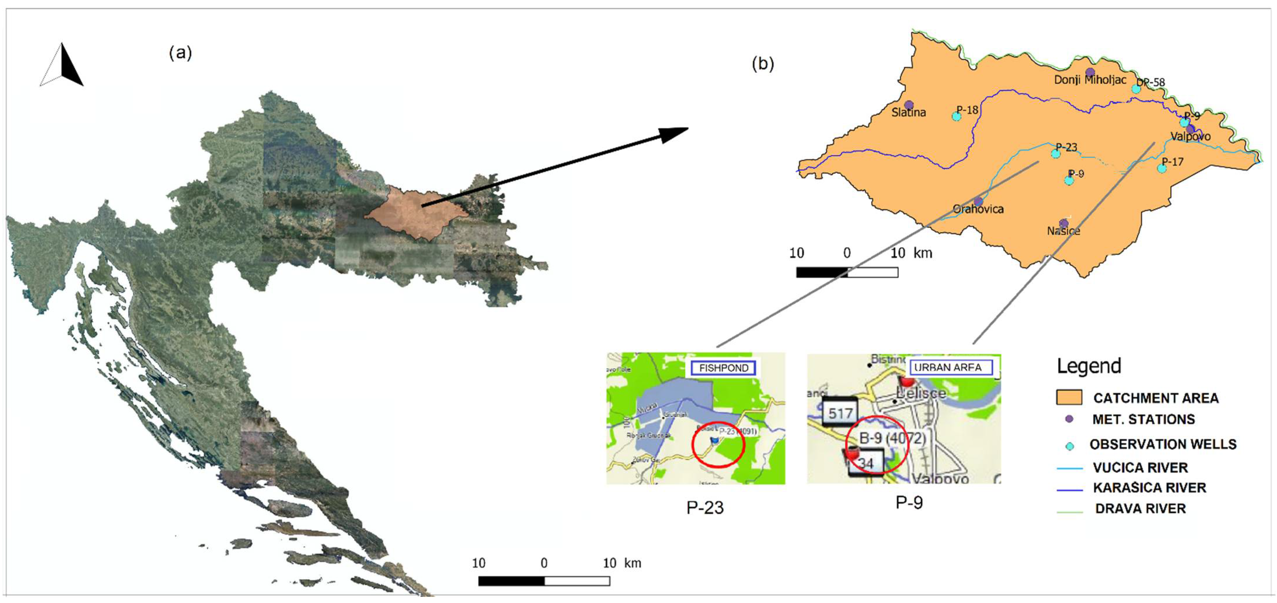
Drought analyses should be conducted in catchments with minimum anthropogenic impacts over a longer period to obtain reliable results [35]. In this study, a small catchment of the Karašica and Vučica rivers in northern Croatia was selected. The catchment is located in the continental part of Croatia, which belongs to the Danube River basin and its tributary, the Drava River sub-basin. It consists of hilly and lowland areas, mainly under agricultural usage. Based on hydrological and geological characteristics, the downstream part of the catchment is considered a perennial stream with a porous aquifer. It is divided into two sub-catchments of almost equal size (Figure 1).
Both sub-catchments were recognized as almost natural, with minimum human impact on the hydrological regime (small portion of irrigation land, no new constructed reservoirs or water abstractions, etc.) and steady land use and vegetation cover [35].
In this part of Croatia, more frequent drought episodes and warming started in 1988 [36].
Severe droughts occurred in 2000 and 2003, but one of the most extreme droughts was in 2011/2012. In the continental region, its duration was extremely long, with the highest magnitudes since the beginning of the twentieth century [37]. Particularly, this catchment area was characterized by an increasing trend in air temperatures and, at the same time, variability of the precipitation regime [38].
Climate change models predict future warming, especially for summer, in all Croatian regions [39].
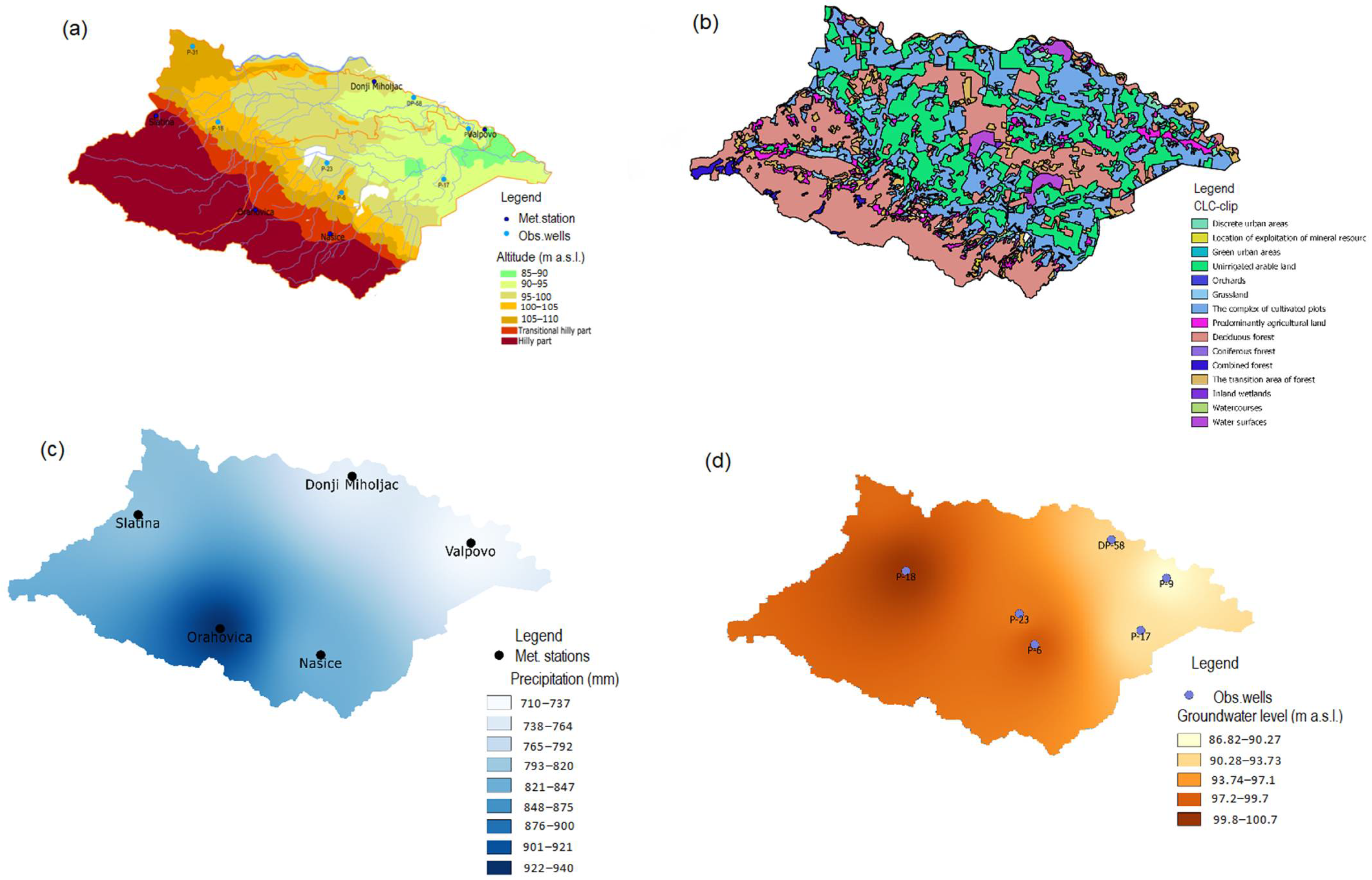
The first small sub-catchment, the Karašica River catchment, has dominant lowland characteristics with a porous aquifer and a small average longitudinal slope (0.011%) (Figure 2a, Table 1). It mostly consists of agricultural land (over 50%), pastures, and forests (Figure 2b) [35].
The data showed on Figure 2 were interpolated by IDW method (inverse distance weighting) by QGIS computer program. IDW interpolation gives weights to sample points, such that the influence of one point on another declines with distance from the new point being estimated. Interpolation results are shown as a two-dimensional raster layer (QGIS Documentation v:3.22. https://docs.qgis.org/3.22/en/docs/gentle_gis_introduction/spatial_analysis_interpolation.html, accessed on 1 February 2022)
Figure 2c depicts the average annual precipitation from 1987 to 2018. The annual precipitation varied between 710 mm at 97.0 m above sea level, and 922 mm at 180.0 m above sea level, at the five meteorological sites. From 1987 to 2018, groundwater levels were recorded at six observation wells in the lowest part of the basin. Figure 2d depicts the average annual groundwater level during the observation period.
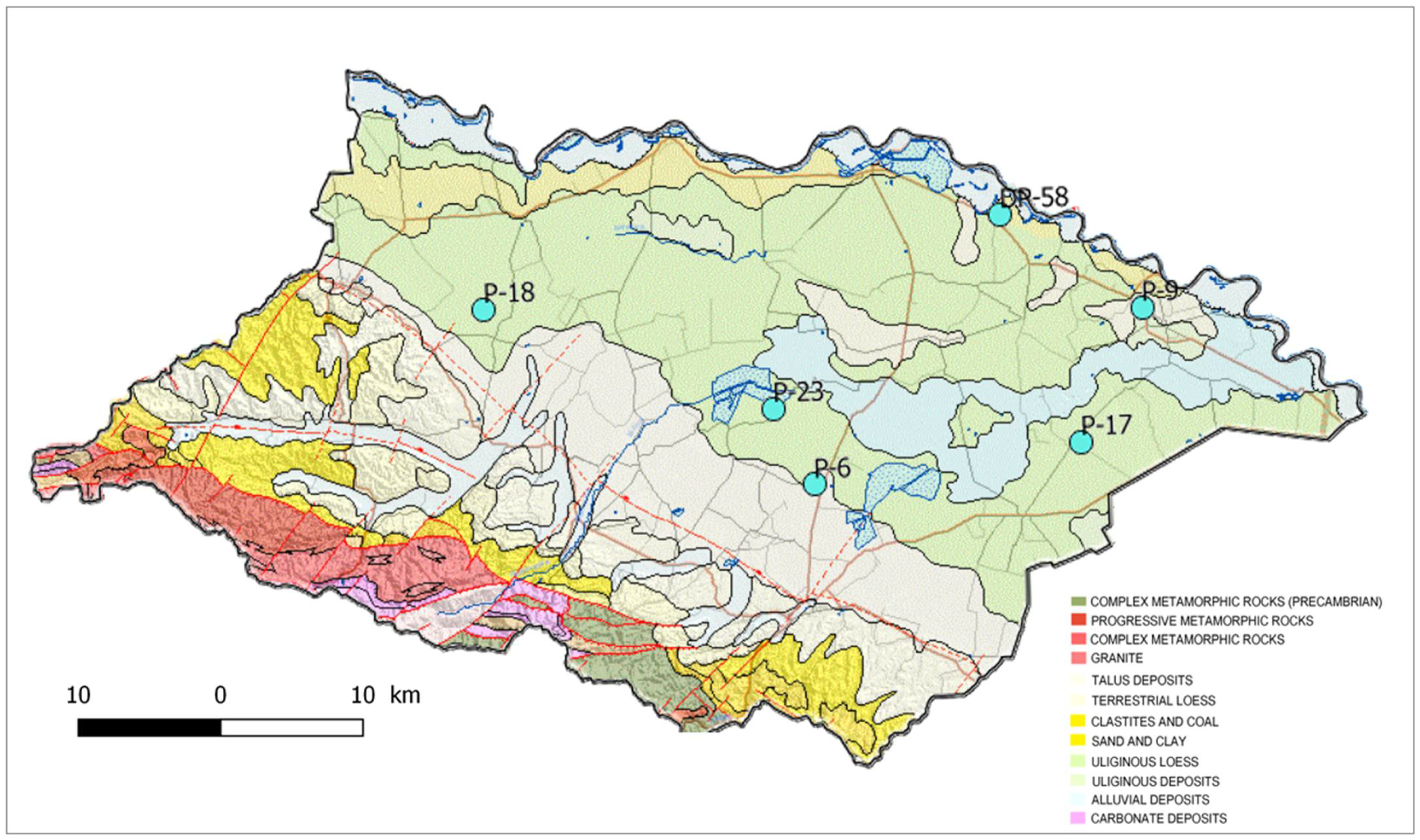
The rest of the catchment is mostly hilly and dominated by forests. Geological characteristics of the study area are exceptionally important for the analysis of hydrological (groundwater) drought. Figure 3 presents the geological catchment map (http://webgis.hgi-cgs.hr/gk300, accessed on 18 March 2022). Most of the lowland area consists of alluvial deposits of different permeability.
3. Materials and Methods
3.1. Input Data
Meteorological and hydrological data used in further analyses of drought indices were provided by the Croatian Meteorological and Hydrological Service, https://meteo.hr/index_en.php (accessed on 15 January 2022). Monthly precipitation data for the period 1987–2018 from five meteorological stations were used for the meteorological drought index. Hydrological drought indices were calculated based on the daily groundwater levels (GW) of six observation wells. These are shown in Figure 1. The positions of the observation wells and average annual groundwater levels for the period 1987–2018 are given in Table 2. Altitude “0” refers to the bottom of the observation well.
3.2. Standardized Precipitation Index (SPI)
The SPI, which is the approach most widely used in all parts of the world, regardless of meteorological or topographical conditions, was used to analyze meteorological drought. Each dataset was fitted to the gamma function to define the relationship between probability and precipitation. Once the relationship of probability to precipitation was established from the historical records, the probability of any observed precipitation data point was calculated and used, along with an estimate of the inverse normal, to calculate the precipitation deviation for a normally distributed probability density with a mean of zero and a standard deviation of unity [23]. Negative SPI and SPEI values indicated mild to extremely dry periods (Table 3). The same index can be used to evaluate drought severity in various water resources (groundwater, open watercourses, and soil moisture) depending on the purpose of the drought analysis. Time scales of 1–6 months are appropriate for the analysis of drought in agriculture, 1–2 months are needed for meteorological drought, and 6–24 months are needed for hydrological drought.
The results of the 1, 3, 6, 12, 24, and 48 month SPI calculations for the period 1981–2018 are given in the Supplementary Materials. Extreme droughts of short periods (1, 3, and 6 months) with SPI values < −2.0 occasionally occurred during the complete observation period. The 24 and 48-month SPIs occurred at the end of the 1990s over a longer period.
3.3. Standardized Precipitation Evapotranspiration Index (SPEI)
The SPEI was proposed by Vicente–Serrano [24]. It is based on the same calculation as the SPI, which uses the normalized gamma distribution of precipitation and provides a number of standard deviations with regard to an average value. The only difference is that precipitation is replaced by the difference between precipitation and potential evapotranspiration. The classification of SPI and SPEI values are the same and are shown in Table 3. Potential evapotranspiration was calculated based on the Thornthwaite equation. The SPEI results are provided in the Supplementary Materials.
3.4. Standardized Groundwater Level Index (SGI)
Groundwater flow is complex process, and it is difficult to obtain direct observational data related to groundwater resources [32]. Water accumulation in the soil, nonetheless, is an important water balance component that has a significant impact on agriculture and water use. SPI is a good technique for groundwater drought evaluation when applied to groundwater level data from a specific area under standard set conditions with variable accumulation times. The time periods required to achieve a maximum correlation exhibit high spatial variability (ranging from 3 to 36 months) [41]. The interpretation of the resulting SGI must reflect an appreciation of the hydrogeological environment of the observation borehole, because SGI can be strongly influenced by site-specific recharging [29]. This approach is similar to the standardized water level index (SWI), with certain adjustments [42]. Since ground water level is measured down from the surface, positive anomalies correspond to drought and negative anomalies correspond to wet or normal conditions. To avoid this approach, we used water depth data measured from the bottom of each observation well:
where Gij represents monthly water level of i-th well and j-th observation, Gim is the mean value of the data series, and σ is its standard deviation.
3.5. Correlation Function
Correlations of SPI and SPEI, SPI and SGI, and SPI and GW, between 1 and 48 months were calculated using the Pearson correlation method [43]:
where N represents the number of data points in each data series, and xi and yi are data points in the first and second data series, respectively.
The Pearson correlation method has been recognized as the most appropriate, compared with the Kendall and Spearman correlation functions [44]. According to the physical processes of surface runoff and percolation into the soil, a temporal delay between the precipitation and water balancing components is necessary. After a certain period, rainfall deficiency and drought consequences are recognized as below-average storage conditions in surface water, reservoirs, and groundwater [41]. As a result, hydrological drought forecasting has become more complicated and unreliable.
Another study concluded that SGI values correlated well with SPI values that were observed 5–8 months ago [45].
4. Results and Discussion
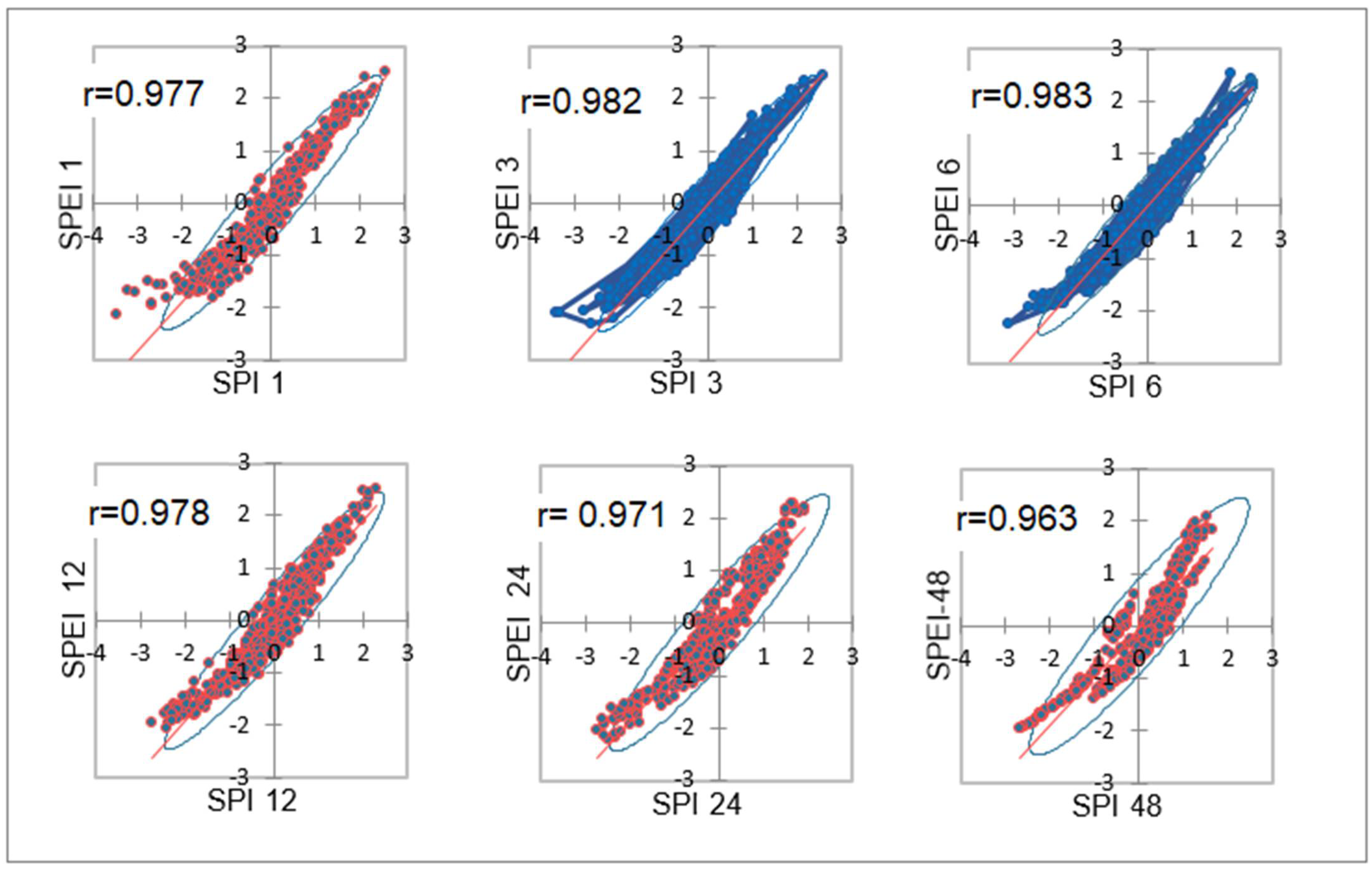
Meteorological drought indices, standardized precipitation index and standardized precipitation evapotranspiration index were compared, in order to define their reliability for further analysis. We calculated their correlations over different time scales (1 to 48 months). The results are presented in Figure 4, showing a very high level of correlation.
All SPI/SPEI correlation values were very high, between 0.963 and 0.983. The highest values of Pearson correlation coefficients were obtained for 3 and 6 month timescales. The other basic statistic parameters, such as index of agreement (d), mean absolute error (MAE), root mean square error (RMSE), mean bias error (MBE), trendline equation (slope and intercept) and determination coefficient (R2) also confirmed high correspondence between all SPI and SPEI values (Table 4). This result led us to the conclusion that application of SPI in further analyses gives acceptable accuracy.
Additionally, we calculated SPI/SPEI correlations over different time scales (1 to 48 months) for Našice and Slatina meteorological stations. Results are given in the Supplementary materials, showing a very high level of correlation (0.82–0.881, and 0.935 and 0.981, respectively). Two other two meteorological stations (Orahovica and Valpovo) had long periods of missing data in air temperature data series, and the SPEI could not be calculated.
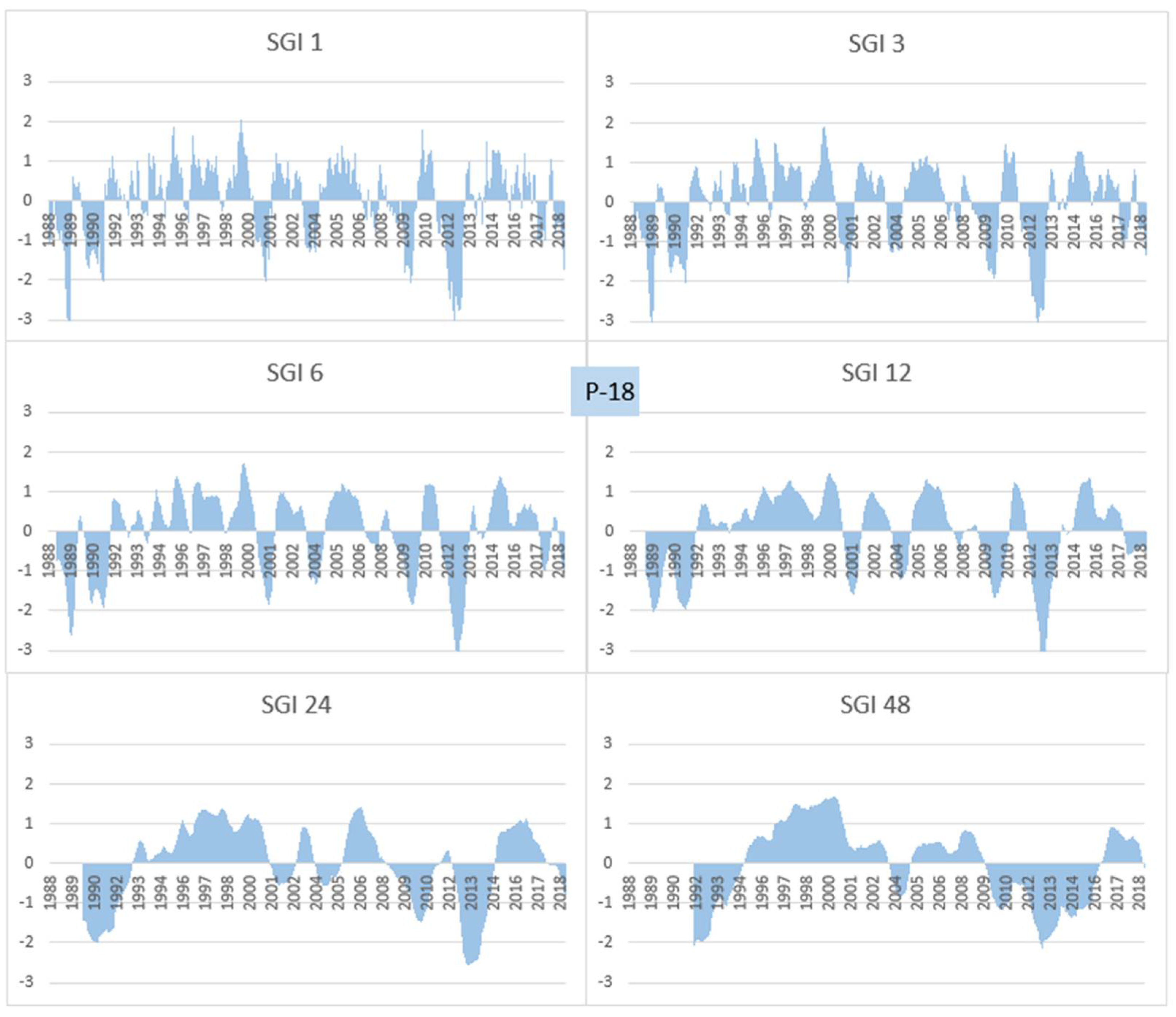
Figure 5 presents the 1, 3, 6, 12, 24, and 48 month SGI values calculated for one observation well, P-18. Pronounced severe drought periods of all analyzed time scales occurred in the 1990s. The SGI results calculated for the other five observation wells are provided in the Supplementary Materials.
The SPI calculation procedure only requires precipitation data, which are almost always available. Hydrological drought deficits are influenced by average catchment wetness (mean annual precipitation) and elevation (reflecting seasonal storage in the snowpack and glaciers), both of which are governed by a complex combination of climate and catchment characteristics, including catchment storage capacity [29].
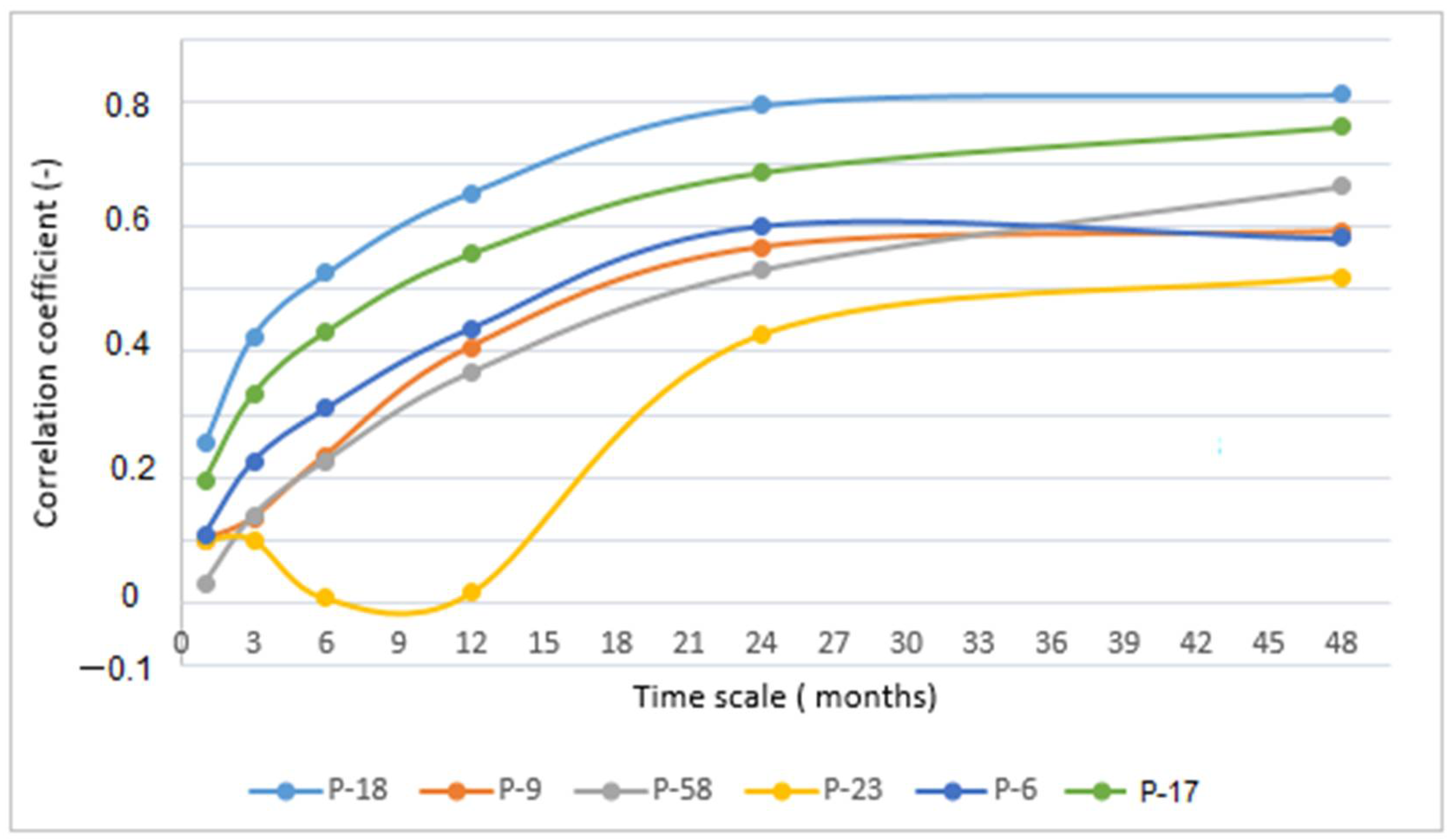
The correlation between the SPI and standardized groundwater index (SGI) was highest at the longest time scale (48 months) for all observation wells. Correlations between SPI and SGI ranged between 0.52 and 0.82, as shown in Figure 6.
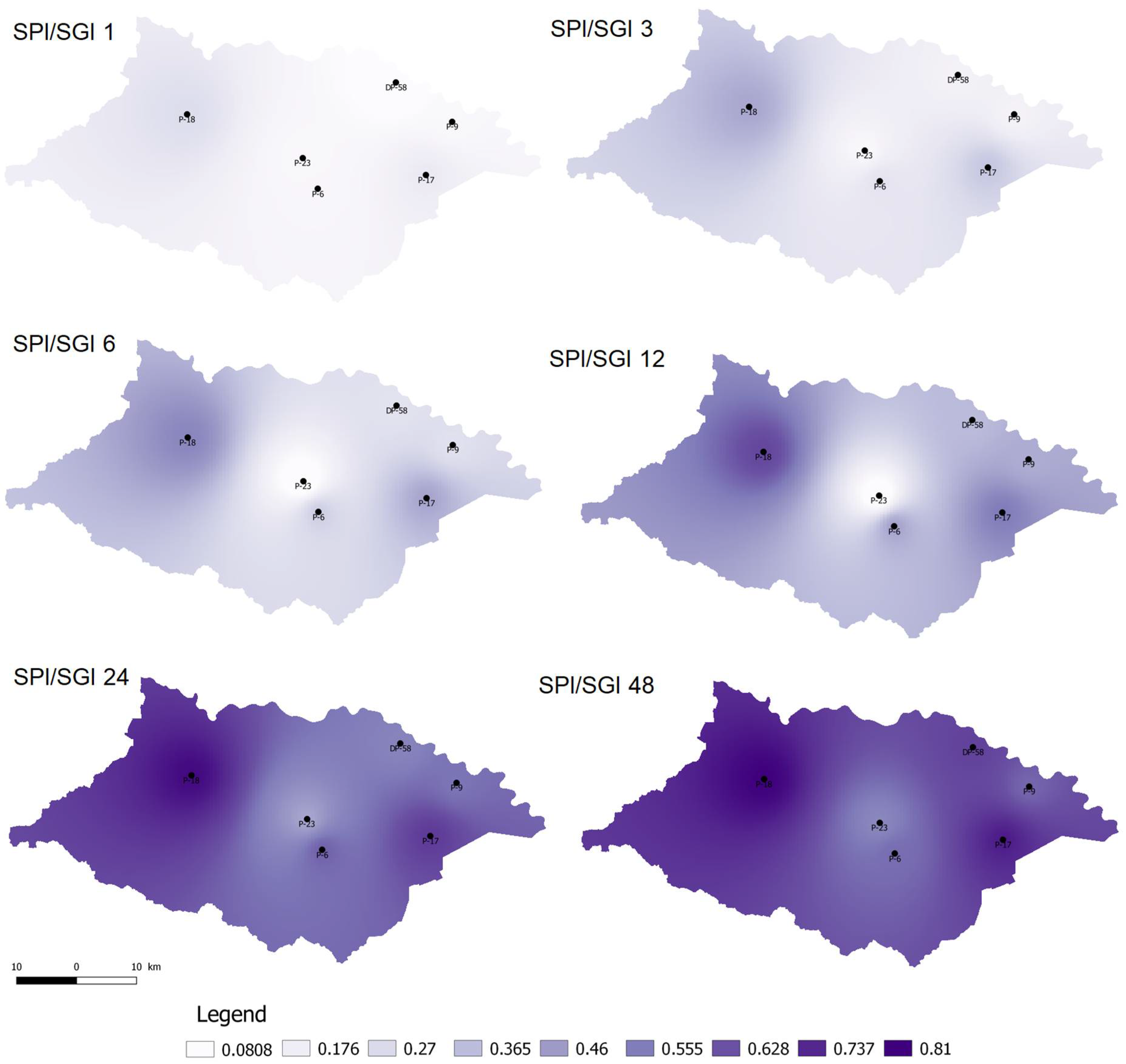
Calculated SGI was correlated to the SPI of the nearest meteorological station. The SPI/SGI correlation coefficients for most observation wells were continuously increasing over different time scales. Only P-23 exhibited a typical behavior. According to Table 2, it is a shallow piezometer located close to the fishpond (Figure 1), and its groundwater table was strongly impacted by surface water. It exceeded the maximum SPI/SGI correlation at the 48 month time scale, similar to the others, but the correlation coefficient at the 1 month scale was higher than on the 6 and 12 month scales. Very high correlation coefficients for P-18 were only at the 24 and 48 month scales, and for P-17 at the 48 month scale. For the other wells, except for P-23, the correlations were moderate at 24 and 48 months. The spatial distributions of the calculated SPI/SGI correlations over different time scales are presented in Figure 7. The highest values of the correlation function for all observation wells were at the longest time scale (48 months), with very high correlation coefficients.
As stated earlier, the catchments are situated in lowland Holocene river terraces, with the lowest parts at 80–120 m above sea level. They are built up from fluvial sediments of variable thickness, permeability, and composition (gravel, sand, silt, or clay) belonging to Gleysols, Fluvisols, and sporadically, other hydromorphic soils characterized by large clay content [46].
Input data for mapping SPI/SGI correlations are in given in the Supplementary Materials.
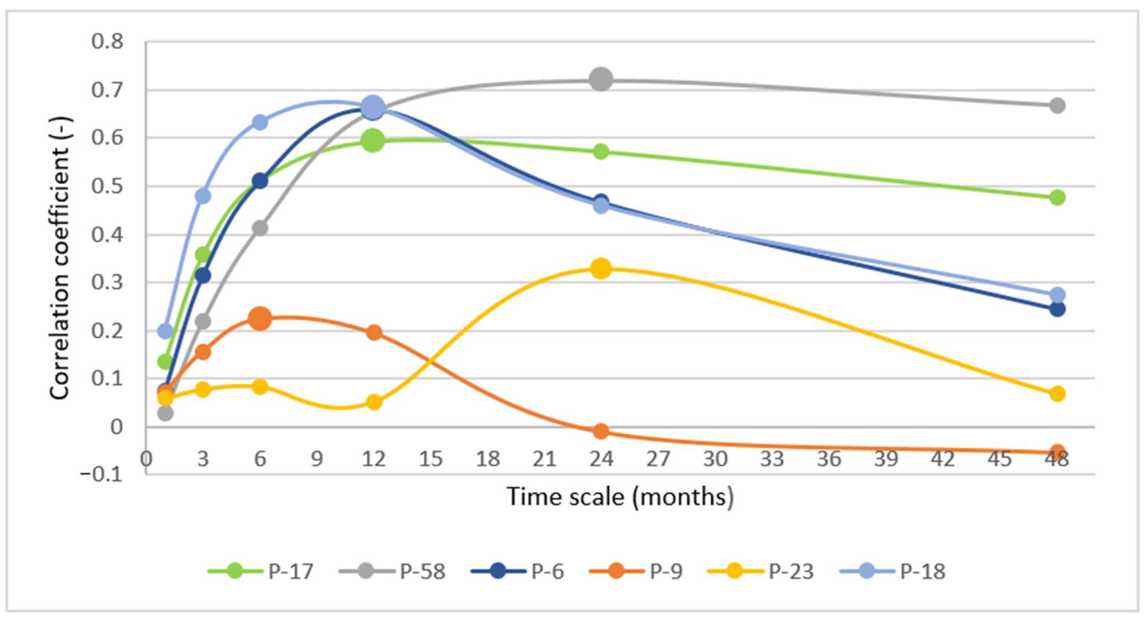
Further application of correlation analysis on SPI and groundwater levels (GW) showed a different relationship (Figure 8). The results showed that the curves of most correlation coefficients followed the same pattern (P-17, P-6 and P-18). Each curve in this group increased as it reached the correlation peak (0.6 to 0.66) in 12 months, and then slowly decreased to values between 0.25 and 0.48. Observation well P-58 had the highest correlation peak (0.72), which appeared much later, after 24 months. Observation well P-9 had the lowest SPI/GW correlation coefficient; the maximum value was 0.22 and it appeared in a short time period, after 6 months. After that, its correlation curve dropped to negative values. According to Table 2, it is a deep piezometer located in the urban area, close to the river (Figure 1), and its groundwater table was probably impacted by soil structure and surface water.
Observation well P-23 exhibited similar behavior as in SPI/SGI correlation analysis. According to Table 2, it is a shallow piezometer located close to the fishpond (Figure 1), and its groundwater table was strongly impacted by surface water. It exceeded the maximum SPI/GW correlation at the 24 month time scale (0.33) but its correlation coefficient curve was completely different.
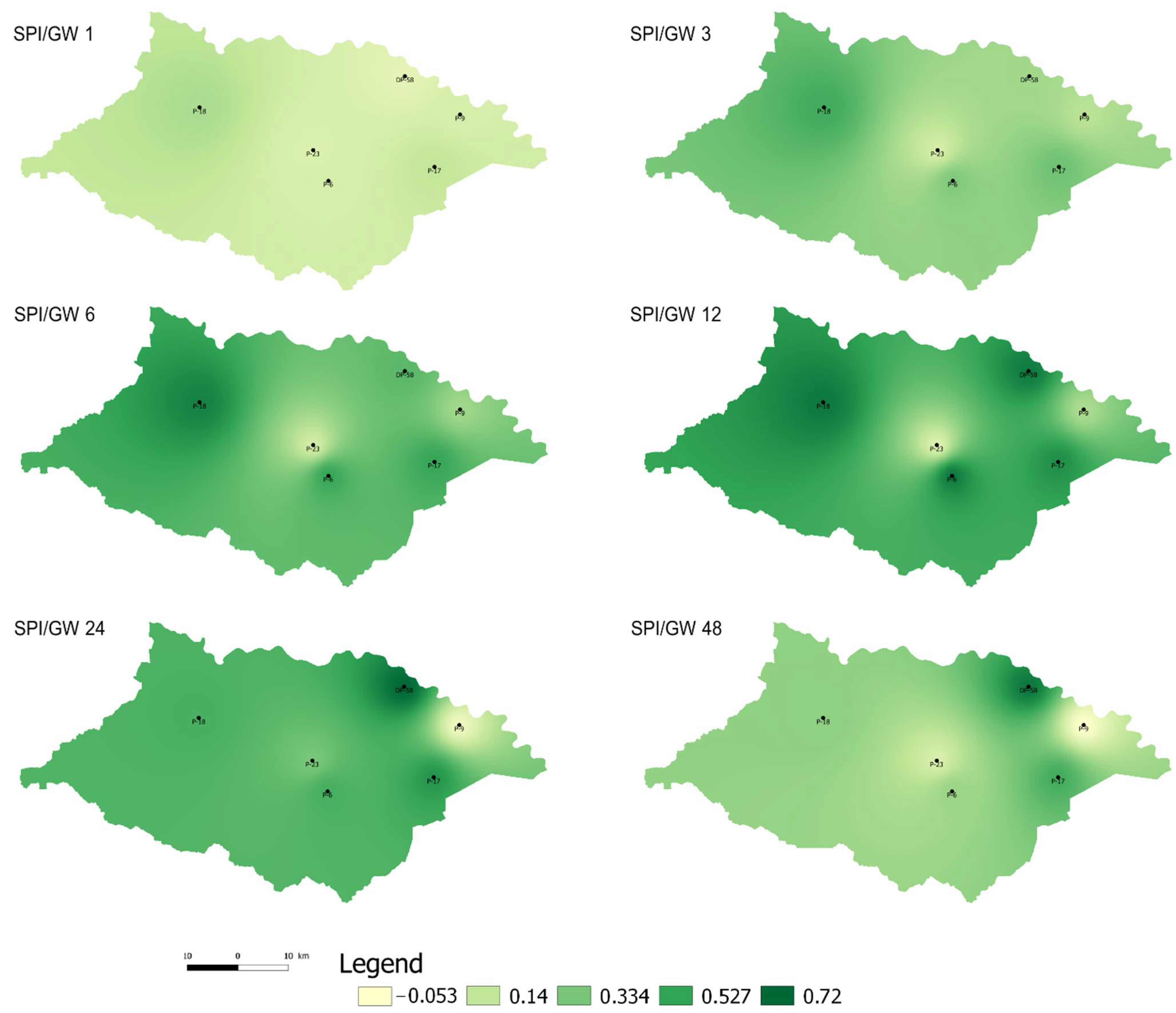
In order to check their correlation uniformity, we introduced SPI/GW (groundwater level) correlation analysis [44]. SPI/GW correlation analysis was performed in order to examine the relationship between meteorological drought and groundwater level. The spatial distributions of the calculated SPI/GW correlations over different time scales are presented in Figure 9. Compared with Figure 7, the maximum correlation coefficients for most observation wells appeared over a shorter time period, 12 and 24 months. Input data for mapping SPI/GW correlations are in given in the Supplementary Materials.
Observed results showed lower and more variable correlation values. The correlation between the SPI and groundwater level (GW) was the highest at different time scales (6 to 24 months) for all observation wells. Maximum correlations between SPI and GW ranged between 0.22 and 0.72, as shown in Figure 8. The correlation coefficients showed much higher variability related to the position and depth of observation wells. Again, only shallow observation well P-23 had specific behavior because of its dependence on surface water (fishpond). Its SPI/GW correlation coefficients were, compared with others, very low. Additionally, P-9 had a relatively low correlation (even negative) with meteorological drought, due to its position in the urban area, very close to the Karašica River. It is a deep observation well and it was probably strongly impacted by deeper aquifers (Figure 1).
5. Conclusions
According to the analysis of meteorological and groundwater drought, it can be concluded that the SPI and SGI correlations are significant over a longer time scale. The study area is located in Danubian valley and is characterized by multi-layered alluvial lowland.
The time taken for rainwater to accumulate in the subsurface and percolate into deeper layers is important for detecting groundwater shortages. Hydrological drought can take up to 36 months to manifest, compared with meteorological conditions, according to published research [17].
In addition, in regions with a carbonate basement, the delay is much less, only 18 months [44,47]. However, the behavior of groundwater is complex, which confirms this finding. In this research, groundwater drought, expressed by SGI, is about 48 months’ delayed. The lag impact on the SGI revealed variations, since groundwater level is influenced by a variety of hydraulic and hydrological phenomena. The correlation between the SPI and standardized groundwater index (SGI) was the highest at the longest time scale (48 months) for all observation wells. Correlations between SPI and SGI ranged between 0.52 and 0.82, as shown in Figure 6. The observed area was only 2000 km2, approximately, but SPI/SGI curves had almost the same shape, with the exception of P-23 (Figure 6).
Correlation coefficients showed similar behavior related to position and depth of observation wells. Only shallow observation well P-23 showed specific behavior because of its dependence on surface water (fishpond). Its SPI/SGI correlation coefficients were the lowest.
The results confirmed that groundwater response to drought and its changes over time are very site specific, and observations are, therefore, hardly scalable from point to catchment scale [48].
Drought, particularly hydrological drought, is a complicated phenomenon. The size of the catchment area greatly affects the accuracy of drought classification. This is especially evident in groundwater drought analysis, where the location of observation wells, their height/depth, proximity to water bodies, geological properties, and other factors significantly impact drought classification. In addition, meteorological drought severity, compared with hydrological droughts, is much more complex. Groundwater drought has a long delay period and lasts for decades. Therefore, predicting hydrological drought based on meteorological data is highly risky and unreliable.
Supplementary Materials
The following supporting information can be downloaded at: https://0-www-mdpi-com.brum.beds.ac.uk/article/10.3390/hydrology9050079/s1, Figure S1: Standardised precipitation index over different time periods (1, 3, 6, 12, 24 and 48 months) for Donji Miholjac meteorological station; Figure S2: Standardised precipitation evapotranspiration index over different time periods (1, 3, 6, 12, 24 and 48 months) for Donji Miholjac meteorological station; Figure S3: Standardised groundwater index over different time periods (1, 3, 6, 12, 24 and 48 months) for P-58 observation well; Figure S4: Standardised groundwater index over different time periods (1, 3, 6, 12, 24 and 48 months) for P-18 observation well; Figure S5: Standardised groundwater index over different time periods (1, 3, 6, 12, 24 and 48 months) for P-23 observation well; Figure S6: Standardised groundwater index over different time periods (1, 3, 6, 12, 24 and 48 months) for P-6 observation well; Figure S7: Standardised groundwater index over different time periods (1, 3, 6, 12, 24 and 48 months) for P-9 observation well; Figure S8: Standardised groundwater index over different time periods (1, 3, 6, 12, 24 and 48 months) for P-17 observation well; Figure S9: Correlation between SPI and SPEI in different time scales (Našice meteorological station); Figure S10: Correlation between SPI and SPEI in different time scales (Slatina meteorological station); Table S1: Data base of spatial distribution of SPI/SGI correlation over different time scales presented in Figure 7; Table S2: Data base of spatial distribution of SPI/SGI correlation over different time scales presented in Figure 9.
Author Contributions
Conceptualization, T.B.; methodology, T.B. and L.T.; data analysis, L.T. and T.B.; writing—original draft preparation, T.B. and L.T.; writing—review and editing, L.T. and T.B. All authors have read and agreed to the published version of the manuscript.
Funding
This research received no external funding.
Institutional Review Board Statement
Not applicable.
Informed Consent Statement
Not applicable.
Data Availability Statement
Not applicable.
Conflicts of Interest
The authors declare no conflict of interest.
References
- Van Loon, A.F. Hydrological drought explained. WIREs Water 2015, 2, 359–392. [Google Scholar] [CrossRef]
- Wilhite, D.A.; Glantz, M.H. Understanding the drought phenomenon: The role of definitions. Water Int. 1985, 10, 111–120. [Google Scholar] [CrossRef] [Green Version]
- Koffi, B.; Kouadio, Z.A.; Kouassi, K.H.; Yao, A.B.; Sanchez, M.; Kouassi, K.L. Impact of Meteorological Drought on Streamflows in the Lobo River Catchment at Nibéhibé, Côte d’Ivoire. J. Water Resour. Prot. 2020, 12, 495–511. [Google Scholar] [CrossRef]
- Blöschl, G.; Hall, J.; Viglione, A.; Perdigão, R.A.P.; Parajka, J.; Merz, B.; Lun, D.; Arheimer, B.; Aronica, G.T.; Bilibashi, A.; et al. Changing climate both increases and decreases European river floods. Nature 2019, 573, 108–111. [Google Scholar] [CrossRef] [PubMed]
- Masseroni, D.; Camici, S.; Cislaghi, A.; Vacchiano, G.; Massari, C.; Brocca, L. 65-year changes of annual streamflow volumes across Europe with a focus on the Mediterranean basin. Hydrol. Earth Syst. Sci. 2021, 25, 5589–5601. [Google Scholar] [CrossRef]
- Teuling, A.J.; De Badts, E.A.G.; Jansen, F.A.; Fuchs, R.; Buitink, J.; Hoek Van Dijke, A.J.; Sterling, S.M. Climate change, reforestation/afforestation, and urbanization impacts on evapotranspiration and streamflow in Europe. Hydrol. Earth Syst. Sci. 2019, 23, 3631–3652. [Google Scholar] [CrossRef] [Green Version]
- Vicente-Serrano, S.M.; Peña-Gallardo, M.; Hannaford, J.; Murphy, C.; Lorenzo-Lacruz, J.; Dominguez-Castro, F.; López-Moreno, J.I.; Beguería, S.; Noguera, I.; Harrigan, S.; et al. Climate, irrigation, and land-cover change explain streamflow trends in countries bordering the Northeast Atlantic. Geophys. Res. Lett. 2019, 46, 10821–10833. [Google Scholar] [CrossRef] [Green Version]
- Stahl, K.; Hisdal, H.; Hannaford, J.; Tallaksen, L.M.; van Lanen, H.A.J.; Sauquet, E.; Demuth, S.; Fendekova, M.; Jódar, J. Streamflow trends in Europe: Evidence from a dataset of near-natural catchments. Hydrol. Earth Syst. Sci. 2010, 14, 2367–2382. [Google Scholar] [CrossRef] [Green Version]
- Gudmundsson, L.; Tallaksen, L.M.; Stahl, K.; Clark, D.B.; Dumont, E.; Hagemann, S.; Bertrand, N.; Gerten, D.; Heinke, J.; Hanasaki, N.; et al. Comparing large-scale hydrological model simulations to observed runoff percentiles in Europe. J. Hydrometeorol. 2011, 13, 604–620. [Google Scholar] [CrossRef]
- Prudhomme, C.; Parry, S.; Hannaford, J.; Clark, D.B.; Hagemann, S.; Voss, F. How Well Do Large-Scale Models Reproduce Regional Hydrological Extremes in Europe? J. Hydrometeorol. 2011, 12, 1181–1204. [Google Scholar] [CrossRef] [Green Version]
- Lloyd-Hughes, B.; Shaffrey, L.C.; Vidale, P.L.; Arnell, N.W. An evaluation of the spatiotemporal structure of large-scale European drought within the HiGEM climate model. Int. J. Climatol. 2012, 33, 2024–2035. [Google Scholar] [CrossRef] [Green Version]
- Hanel, M.; Rakovec, O.; Markonis, Y.; Máca, P.; Samaniego, L.; Kyselý, J.; Kumar, R. Revisiting the recent European droughts from a long-term perspective. Sci. Rep. 2018, 8, 9499. [Google Scholar] [CrossRef]
- Lorenzo-Lacruz, J.; Garcia, C.; Morán-Tejeda, E. Groundwater level responses to precipitation variability in Mediterranean insular aquifers. J. Hydrol. 2017, 552, 516–531. [Google Scholar] [CrossRef]
- Caloiero, T.; Veltri, S.; Caloiero, P.; Frustaci, F. Drought Analysis in Europe and in the Mediterranean Basin Using the Standardized Precipitation Index. Water 2018, 10, 1043. [Google Scholar] [CrossRef] [Green Version]
- Breuer, H.; Ács, F.; Skarbit, N. Climate change in Hungary during the twentieth century according to Feddema. Theor. Appl. Climatol. 2017, 127, 853–863. [Google Scholar] [CrossRef]
- Vogel, M.M.; Zscheischler, J.; Seneviratne, S.I. Varying soil moisture-atmosphere feedbacks explain divergent temperature extremes and precipitation projections in central Europe. Earth Syst. Dyn. 2018, 9, 1107–1125. [Google Scholar] [CrossRef] [Green Version]
- Ács, F.; Takács, D.; Breuer, H.; Skarbit, N. Climate and climate change in the Austrian–Swiss region of the European Alps during the twentieth century according to Feddema. Theor. Appl. Climatol. 2018, 133, 899–910. [Google Scholar] [CrossRef]
- Hellwig, J.; Stahl, K. An assessment of trends and potential future changes in groundwater-baseflow drought based on catchment response times. Hydrol. Earth Syst. Sci. 2018, 22, 6209–6224. [Google Scholar] [CrossRef] [Green Version]
- Chiang, F.; Mazdiyasni, O.; AghaKouchak, A. Evidence of anthropogenic impacts on global drought frequency, duration, and intensity. Nat. Commun. 2021, 12, 2754. [Google Scholar] [CrossRef]
- Spinoni, J.; Naumann, G.; Carrao, H.; Barbosa, P.; Vogt, J. World drought frequency, duration, and severity for 1951–2010. Int. J. Climatol. 2014, 34, 2792–2804. [Google Scholar] [CrossRef] [Green Version]
- Cook, B.I.; Mankin, J.S.; Marvel, K.; Williams, A.P.; Smerdon, J.E.; Anchukaitis, K.J. Twenty-first century drought projections in the CMIP6 forcing scenarios. Earth’s Future 2020, 8, e2019EF001461. [Google Scholar] [CrossRef] [Green Version]
- Zhao, C.; Brissette, F.; Chen, J.; Martel, J.L. Frequency change of future extreme summer meteorological and hydrological droughts over North America. J. Hydrol. 2020, 584, 124316. [Google Scholar] [CrossRef]
- McKee, T.B.; Doeskin, N.J.; Kleist, J. Drought Monitoring with Multiple Time Scales. In Proceedings of the 9th Conference on Applied Climatology, Dallas, TX, USA, 15–20 January 1995; pp. 233–236. [Google Scholar]
- Vicente-Serrano, S.; Beguaria, S.; López-Moreno, J.I. A Multiscalar Drought Index Sensitive to Global Warming: The Standardized Precipitation Evapotranspiration Index. J. Clim. 2010, 23, 1696–1718. [Google Scholar] [CrossRef] [Green Version]
- Tirivarombo, S.; Osupile, D.; Eliasson, P. Drought monitoring and analysis: Standardised Precipitation Evapotranspiration Index (SPEI) and Standardised Precipitation Index (SPI). Phys. Chem. Earth 2018, 106, 1–10. [Google Scholar] [CrossRef]
- Hisdal, H.; Stahl, K.; Tallaksen, L.M.; Demuth, S. Have streamflow droughts in Europe become more sever or frequent? Int. J. Climatol. 2001, 21, 317–333. [Google Scholar] [CrossRef]
- Peña-Angulo, D.; Vicente-Serrano, S.M.; Domínguez-Castro, F.; Noguera, I.; Tomas-Burguera, M.; López-Moreno, J.I.; Lorenzo-Lacruz, J.; El Kenawy, A. Unravelling the role of vegetation on the different trends between climatic and hydrologic drought in headwater catchments of Spain. Anthropocene 2021, 36, 100309. [Google Scholar] [CrossRef]
- Han, Z.; Huang, S.; Huang, Q.; Leng, G.; Liu, Y.; Bai, Q.; He, P.; Liang, H.; Shi, W. GRACE -based high-resolution propagation threshold from meteorological to groundwater drought. Agric. For. Meteorol. 2021, 307, 108476. [Google Scholar] [CrossRef]
- Bloomfield, J.P.; Marchant, B.P. Analysis of groundwater drought using a variant of the Standardised Precipitation. Hydrol. Earth Syst. Sci. Discuss. 2013, 10, 7537–7574. [Google Scholar]
- Van Loon, A.F.; Laaha, G. Hydrological drought severity explained by climate and catchment characteristics. J. Hydrol. 2015, 526, 3–14. [Google Scholar] [CrossRef] [Green Version]
- Fleig, A.K.; Tallaksen, L.M.; Hisdal, H.; Demuth, S. A global evaluation of streamflow drought characteristics. Hydrol. Earth Syst. Sci. 2006, 10, 535–552. [Google Scholar] [CrossRef] [Green Version]
- Guo, M.; Yue, W.; Wang, T.; Zheng, N.; Wu, L. Assessing the use of standardized groundwater index for quantifying groundwater drought over the conterminous US. J. Hydrol. 2021, 598, 126227. [Google Scholar] [CrossRef]
- Beguería, S.; López-Moreno, J.I.; Lorente, A.; Seeger, M.; García-Ruiz, J.M. Assessing the effect of climate oscillations and land-use changes on streamflow in the Central Spanish Pyrenees. Ambio 2003, 32, 283–286. [Google Scholar] [CrossRef] [PubMed]
- Fenta, A.A.; Yasuda, H.; Shimizu, K.; Haregeweyn, N. Response of streamflow to climate variability and changes in human activities in the semiarid highlands of northern Ethiopia. Reg. Environ. Chang. 2017, 17, 1229–1240. [Google Scholar] [CrossRef]
- Tadić, L.; Dadić, T.; Leko-Kos, M. Variability of Hydrological Parameters and Water Balance Components in Small Catchment in Croatia. Adv. Meteorol. 2016, 2016, 1393241. [Google Scholar] [CrossRef] [Green Version]
- Bonacci, O. Analiza nizova srednjih godišnjih temperatura zraka u Hrvatskoj. Građevinar 2010, 62, 781–791. [Google Scholar]
- Cindrić, K.; Telišman Prtenjak, M.; Herceg-Bulić, I.; Mihajlović, D.; Pasarić, Z. Analysis of the extraordinary 2011/2012 drought in Croatia. Theor. Appl. Climatol. 2016, 123, 503–522. [Google Scholar] [CrossRef]
- Tadić, L.; Brleković, T.; Hajdinger, A.; Španja, S. Analysis of the Inhomogeneous Effect of Different Meteorological Trends on Drought: An Example from Continental Croatia. Water 2019, 11, 2625. [Google Scholar] [CrossRef] [Green Version]
- Marinović, I.; Cindrić Kalin, K.; Güttler, I.; Pasarić, Z. Dry Spells in Croatia: Observed Climate Change and Climate Projections. Atmosphere 2021, 12, 652. [Google Scholar] [CrossRef]
- Li, B.; Zhou, W.; Zhao, Y.; Ju, Q.; Yu, Z.; Liang, Z.; Acharya, K. Using the SPEI to Assess Recent Climate Change in the Yarlung Zangbo River Basin, South Tibet. Water 2015, 7, 5474–5486. [Google Scholar] [CrossRef] [Green Version]
- Kumar, R.; Musuuza, J.L.; Van Loon, A.F.; Adriaan, J.; Teuling, A.J.; Barthel, R.; Broek, J.T.; Mai, J.; Samaniego, L.; Attinger, S. Multiscale evaluation of the Standardized Precipitation Index as a groundwater drought indicator. Hydrol. Earth Syst. Sci. 2016, 20, 1117–1131. [Google Scholar] [CrossRef] [Green Version]
- Bhuiyan, C. Various Drought Indices for Monitoring Drought Condition in Aravalli Terrain of India. In Proceedings of the XXth ISPRS Congress, Istanbul, Turkey, 12–23 July 2004; pp. 12–23. Available online: http://www.isprs.org/proceedings/XXXV/congress/comm7/papers/243.pdf (accessed on 23 March 2022).
- Berman, J.J. Principles and Practice of Big Data, 2nd ed.; Academic Press: Cambridge, MA, USA, 2018. [Google Scholar]
- Balacco, G.; Alfio, M.R.; Fidelibus, M.D. Groundwater Drought Analysis under Data Scarcity: The Case of the Salento Aquifer (Italy). Sustainability 2022, 14, 707. [Google Scholar] [CrossRef]
- Uddameri, V.; Singaraju, S.; Hernandez, E.A. Is Standardized Precipitation Index (SPI) a Useful Indicator to Forecast Groundwater Droughts?—Insights from a Karst Aquifer. JAWRA 2019, 55, 70–88. [Google Scholar] [CrossRef]
- Rubinić, V.; Ilijanić, N.; Magdić, I.; Bensa, A.; Husnjak, S.; Krklec, K. Plasticity, Mineralogy, and WRB Classification of Some Typical Clay Soils along the Two Major Rivers in Croatia. Eurasian Soil Sc. 2020, 53, 922–940. [Google Scholar] [CrossRef]
- Lorenzo-Lacruz, J.; Vicente-Serrano, S.M.; González-Hidalgo, J.C.; López-Moreno, J.I.; Cortesi, N. Hydrological drought response to meteorological drought in the Iberian Peninsula. Clim. Res. 2013, 58, 117–131. [Google Scholar] [CrossRef] [Green Version]
- Van Loon, A.F.; Kumar, R.; Mishra, V. Testing the use of standardised indices and GRACE satellite data to estimate the European 2015 groundwater drought in near-real time. Hydrol. Earth Syst. Sci. 2017, 21, 1947–1971. [Google Scholar] [CrossRef] [Green Version]
Figure 1.
(a) Remote sensing map of study area, https://geoportal.dgu.hr (accessed on 20 March 2022), (b) catchment area with designated main watercourses and observation wells particularly P-29 and P-9.
Figure 1.
(a) Remote sensing map of study area, https://geoportal.dgu.hr (accessed on 20 March 2022), (b) catchment area with designated main watercourses and observation wells particularly P-29 and P-9.

Figure 2.
(a) Altitude map of the catchment area, (b) vegetation cover, (c) annual precipitation distribution, (d) mean groundwater level.
Figure 2.
(a) Altitude map of the catchment area, (b) vegetation cover, (c) annual precipitation distribution, (d) mean groundwater level.

Figure 3.
Geological map of the catchment area with designated observation wells, (http://webgis.hgi-cgs.hr/gk300/, accessed on 19 March 2022).
Figure 3.
Geological map of the catchment area with designated observation wells, (http://webgis.hgi-cgs.hr/gk300/, accessed on 19 March 2022).

Figure 4.
Correlation between SPI and SPEI in different time scales (Donji Miholjac meteorological station).
Figure 4.
Correlation between SPI and SPEI in different time scales (Donji Miholjac meteorological station).

Figure 5.
SGI values for 1, 3, 6, 12, 24, and 48 months (observation well P-18).

Figure 6.
SPI/SGI correlation in different time scales for six observation wells.

Figure 7.
Spatial distribution of SPI/SGI correlation over different time scales.

Figure 8.
SPI/GW correlation in different time scales for six observation wells.

Figure 9.
Spatial distribution of SPI/GW correlation over different time scales.


Table 1.
Basic catchment characteristics.
| Catchment | Area (km2) | Hmin (m Above Sea Level) | Hmax (m Above Sea Level) | Catchment Slope (%) |
|---|---|---|---|---|
| Karašica (K) | 919 | 85 | 556 | 0.011 |
| Vučica (V) | 1156 | 125 | 953 | 0.012 |
Table 2.
Description of observation wells.
| Observation Well | Gaus–Krüger Coordinates | “0” Altitude (m Above Sea Level) | Average Annual Groundwater Level (m Above Sea Level) |
|---|---|---|---|
| P-6 | X = 5 047 122 Y = 6 058 424 | 96.00 | 97.71 |
| P-9 | X = 5 058 545 Y = 6 531 164 | 86.00 | 86.92 |
| P-18 | X = 5 059 774 Y = 6 486 225 | 98.00 | 100.63 |
| P-17 | X = 5 049 538 Y = 6 526 801 | 88.00 | 89.49 |
| P-23 | X = 5 052 429 Y = 6 505 786 | 94.00 | 95.59 |
| P-58 | X = 5 065 203 Y = 6 521 671 | 89.00 | 90.66 |
Table 3.
Limit values for standardized precipitation index (SPI) and standardized precipitation evapotranspiration index (SPEI). Data from [23,40].
| SPI, SPEI Values | Drought Category |
|---|---|
| 0–(−0.99) | Mild drought |
| (−1.0)–(−1.49) | Moderate drought |
| (−1.5)–(−1.99) | Severe drought |
| ≤(−2.0) | Extreme drought |
Table 4.
Statistic parameters of SPI/SPEI correlation.
| Time Scale (Months) | 1 | 3 | 6 | 12 | 24 | 48 |
|---|---|---|---|---|---|---|
| d | 0.977 | 0.983 | 0.983 | 0.978 | 0.971 | 0.798 |
| MAE | 0.21 | 0.198 | 0.199 | 0.232 | 0.289 | 0.675 |
| RMSE | 0.298 | 0.261 | 0.258 | 0.295 | 0.339 | 0.827 |
| MBE | −0.005 | −0.004 | −0.011 | −0.09 | 0.05 | 0.01 |
| Slope (a) | 0.94 | 0.957 | 0.962 | 0.951 | 0.936 | 0.923 |
| Intercept (b) | 0.0041 | −0.006 | −0.0099 | −0.01 | 0.0019 | −0.011 |
| R2 | 0.913 | 0.933 | 0.935 | 0.915 | 0.89 | 0.861 |
Publisher’s Note: MDPI stays neutral with regard to jurisdictional claims in published maps and institutional affiliations. |
© 2022 by the authors. Licensee MDPI, Basel, Switzerland. This article is an open access article distributed under the terms and conditions of the Creative Commons Attribution (CC BY) license (https://creativecommons.org/licenses/by/4.0/).
Share and Cite
MDPI and ACS Style
Brleković, T.; Tadić, L. Hydrological Drought Assessment in a Small Lowland Catchment in Croatia. Hydrology 2022, 9, 79. https://0-doi-org.brum.beds.ac.uk/10.3390/hydrology9050079
AMA Style
Brleković T, Tadić L. Hydrological Drought Assessment in a Small Lowland Catchment in Croatia. Hydrology. 2022; 9(5):79. https://0-doi-org.brum.beds.ac.uk/10.3390/hydrology9050079
Chicago/Turabian StyleBrleković, Tamara, and Lidija Tadić. 2022. "Hydrological Drought Assessment in a Small Lowland Catchment in Croatia" Hydrology 9, no. 5: 79. https://0-doi-org.brum.beds.ac.uk/10.3390/hydrology9050079
Note that from the first issue of 2016, this journal uses article numbers instead of page numbers. See further details here.