The Development of Explicit Equations for Estimating Settling Velocity Based on Artificial Neural Networks Procedure

Abstract

This study proposes seven equations to predict the settling velocity of sediment particles with variations in grain size (d), particle shape factor (SF), and water temperature (T) based on the artificial neural network procedure. The data used to develop the equations were obtained from digitizing charts provided by the U.S. Interagency Committee on Water Resources (U.S-ICWR) and compiled from the measurement data of settling velocity from several sources. The equations are compared to three existing equations available in the literature and then analyzed using graphical and statistical analysis. The simulation results show the proposed equations produce satisfactory results. The proposed equations can predict the settling velocity of natural particle sediments, with diameters ranging between 0.05 mm and 10 mm in water with temperatures between 0 °C and 40 °C, and shape factor SF ranging between 0.5 and 0.95.

1. Introduction

The settling or fall velocity of sediment particles (W_s) is an important aspect of sediment transport processes, such as suspension, deposition, mixing, and exchange near the bed [1]. It is defined as the average terminal velocity attained by a sediment particle during the settling process in still water [1]. Some of its influencing factors include fluid properties, such as temperature, viscosity, and flow regime as well as sediment characteristics, such as particle size and its shape factor, and submerged specific weight [1,2]. The settling velocity for a single spherical particle, W_s, was studied by applying gravity force, buoyancy, and drag forces during its settling process [1,2]. Due to the hydrodynamic complexity associated with W_s, a correlation is usually proposed between non-dimensional parameters of the drag coefficient C_D and the particle Reynold number Re defined by Equations (1) and (2) [1,3].

$$Re=\frac{W_{s}d}{\vartheta }$$

(1)

$$C_D=\frac{4\left({\rho }_s/{\rho }_f-1\right)dg}{3W_s^2}$$

(2)

where d is the particle diameter, ϑ and ρ_f are the kinematic viscosity and density of the fluid, respectively, ρ_s is the density of sediment, and g = gravity acceleration [1,3]. The original idea of the C_D to Re relationship was Stokes. Stokes derived the drag force on a spherical particle by solving the Navier–Stokes equations without the inertia terms and proposed relationship C_D = 24/Re. This theory was observed to be valid in the laminar region for Re < 0.1. However, the theory fails to accurately predict the settling velocity when the fluid becomes turbulent, thereby, making the turbulent drag important [4]. Oseen and Goldstein (see Wu [1]) improved the Stokes theorem by including the inertia terms in the Navier–Stokes equations to provide the formulas to estimate the settling velocity considered to be valid for the turbulent region. Meanwhile, the sediment particles with irregular shapes, such as those in natural rivers, have rough surfaces and exhibit different characteristics in settling velocity compared to spherical particles.

The hydrodynamic complexity associated with W_s, for nonspherical materials, becomes more complex. The study of settling velocity for nonspherical materials has been carried out for a long time. The effect of particle shape on the settling velocity was studied extensively over sixty years ago using experimental investigation [5,6,7,8,9]. These studies provide a series of graphical relations to estimate the settling velocity of sediment particles for given particle sizes, shape factors, and water temperature [1,2]. The graphic was published by the Subcommittee on Sedimentation of the U.S. Interagency Committee on Water Resources, US-ICWR [10] to determine the settling velocity at different fluid conditions and sediment particles. However, this graphical relationship is inconvenient because some interpolation is required to obtain the desired value [1,11]. Several methods and formulas have been proposed afterward to estimate the sediment settling velocity for spherical and nonspherical particles [11,12,13,14,15,16,17,18,19,20,21,22,23,24,25,26]. Among these formulas, the formula proposed by Wu and Wang [11] was obtained by using more extensive experimental data. They matched the results as closely as possible to the charts from the Interagency Committee. In other words, the formula of Wu and Wang [11] can be said to be an explicit form of the more complete Interagency Committee’s charts.

This study also proposes explicit equations for the Interagency Committee’s charts. In contrast to the development of the Wu and Wang formula [11], the procedures presented in this study directly use the information available on the Interagency Committee’s charts through an artificial neural networks (ANN) approach. The relationship between a number of input and output data can be built through the ANN method. The input data consisting of grain diameter (d), particle shape (SF), water temperature (T), and output (W_s) is taken from the graphics through digitizing the Interagency Committee’s charts. This study uses the Corey shape factor SF which is defined by Equation (3):

$$SF=\frac{c}{\sqrt{ab}}$$

(3)

where a, b, and c are the lengths of the longest, the intermediate, and the shortest mutually perpendicular axes, respectively [1]. This explicit ANN method proposed in this study will be helpful because it can also be applied to obtain sediment parameters that must be obtained through many graphic interpolations found in sediment transport studies. Examples include Shield diagrams to determine the critical bed shear stresses at the bottom regarding the initial motion of particles, some charts related to the C_D and Re relationship for calculating W_s, and other graphics that are widely used in sediment transport studies. The proposed equations in this study were validated and tested through their application to other experimental data on settling velocity compiled from several sources. The equations are also compared to three existing equations to compute the settling velocity of particle sediment considering shape factor SF including those proposed by Jimenez and Madsen [21], Wu and Wang [11], and Camenen [23], for evaluating their performances.

The continuous availability of the dataset as well as the existence of multidimensional and complex non-linear relations in the settling velocity estimation makes the ANN approach feasible as an alternative solution. Artificial neural networks (ANNs) are a computational approach inspired by the neural system of the human brain. They have become very popular in many diverse fields in recent years due to their ability to receive multiple information and provide meaningful solutions to problems with high-level complexity and nonlinearity without requiring the complex nature of the underlying process to be well defined or clearly understood [27,28,29,30]. Moreover, the process of receiving and processing the information of neural networks relies on several non-linear processing elements, such as nodes or neurons [27]. The commonly used and simple neural network model is the Multilayer Perceptron (MLP) which is an architecture arranged in a layered configuration consisting of three main layers which include the input, hidden, and output layers. The ANNs have been successfully used in studies related to hydrologic modeling [31,32,33,34], and for streamflow predictions [35,36,37,38]. Several studies have also successfully applied the method in sediment transport, such as suspended sediment estimations [39,40,41,42,43], prediction of bed sediment load [44,45], and others. However, its application to sediment settling velocity estimation is quite limited as observed in Seyed Mortez et al. [46], Goldstein and Coco [4], and Rushd et al. [3]. Seyed Mortez et al. [46] developed an ANN model to predict the settling velocity of natural sediment and compared the results with the experimental and existing formulas from the previous study. It was discovered that the ANN model has more prediction ability than the available formulas. Goldstein and Coco [4] also developed a genetic programming (GP) algorithm in an ANN model to predict the settling velocity of non-cohesive sediment and found that the GP models improved the results better compared to the formulas of Dietrich [17] and Ferguson and Church [22]. It was concluded that the GP models ideally capture the complex and non-linear properties of the input variables considered, such as the nominal diameter of the sediment, kinematic viscosity of the fluid, and submerged specific gravity of the sediment. Moreover, Rushd et al. [3] predicted the settling velocity of spherical particles using MLP based methodology for both the Newtonian and the non-Newtonian fluids (Power-law, Bingham Plastic, and Herschel Bulkley models) and showed that MLP has a good performance, thereby, making it an effective and accurate prediction tool for the settling velocity in both fluid conditions. It should be noted that the ANN procedure involves implicit operations, and this makes it difficult for those not familiar with the system to understand and apply it to practical studies. Therefore, this study proposes five explicit equations of the ANN algorithm to ensure their easy application and integration into other existing programs dealing with sediment transport and settling velocity computations.

The ANNs can also be treated as a universal approximator with the ability to learn the complex nature of the underlying process under consideration without it being explicitly defined in a mathematical form [47,48]. It was, therefore, considered an approximation method in this study for the three-dimensional function of the settling velocity with three independent variables which include sediment grain size (d), shape (SF), and fluid temperature (T) or kinematics viscosity ϑ. In this case, the graphical form of the settling velocity function is known which is the Interagency Committee’s charts while its mathematical equation needs to be determined using the ANN procedure.

The main objective of this study is to determine equations that describe an explicit neural network formulation to estimate the settling velocity of sediment particles. Five equations are proposed in this study. The first and second equations of settling velocity are related directly to sediment and fluid parameters as the input, such as the sediment size (d), shape factor (SF), and water temperature (T). The third to fifth equations use shape factor SF and non-dimensional diameter parameter $D_{*}$ defined by Equation (4) as the input parameters and particle Reynold number Re or drag coefficient C_D as the output parameter while setting velocity is determined from Re and C_D.

$$D_{*}=d {\left[\frac{g\left({\rho }_s/{\rho }_f-1\right)}{{\vartheta }^2}\right]}^{1/3}$$

(4)

The following section of this paper will describe the materials and methods used in developing the equations. The compilation of the data needed for training, validation, and testing is described in the data description, then the method is given to specify the ANN structure and the method used for transforming the ANN model into explicit equations to determine the settling velocity as a function of sediment and fluid characteristics. Then, the section is followed by the simulation results of the ANN models and a comparison with existing formulas will be discussed. Examples for the use of procedures and the conclusion are also given.

2. Materials and Methods

2.1. Data Description

The data for training and validation of the model were obtained by digitizing the Interagency Committee’s charts using WebPlotDigitizer software (https://automeris.io/WebPlotDigitizer/, accessed on 20 August 2021). The digitization process produced 520 data points with nominal diameter of the sediment particle (d) ranging from 0.06 mm to 10 mm, water temperature (T) from 0 °C to 40 °C, shape factor of the sediment particle (SF) from 0.5 to 0.9, and settling velocity (W_s) from 0.177 cm/s to 50.67 cm/s. From these digitized data, 350 were used for training and 86 for validation, and 84 for testing (testing 1). The measurement data from several available sources were used in another testing model (testing 2), as indicated in

Table 1. Data used for training, validation, and testing ANN Models.

Source Number	Source	Data Using	Data Point	Range of Fluid and Sediment Parameters
1	U.S. Inter-Agency Committee [10]; data obtained by digitizing charts.	training & validation	359, 86	d: 0.06 mm to 10 mm, T: 0 °C to 40 °C, SF: 0.5 to 0.9 and Ws: 0.177 cm/s to 50.67 cm/s.
		testing 1	84
2	Schultz et al. [9]	testing 2	121	d: 0.19 mm to 1.6 mm, T: 13.5 °C to 19.5 °C, SF: 0.34 to 0.99 and Ws: 1.6 cm/s to 16.35 cm/s.
3	Cheng [20]	testing 2	38	d: 0.061 mm to 10.0 mm, T: 7.5 °C to 20 °C, SF: 0.7 and Ws: 0.235 cm/s to 44.54 cm/s.
4	Smith and Cheung [49]	testing 2	22	d: 0.42 mm to 6.91 mm, T: 20.0 °C, SF: 0.29 to 0.977 and Ws: 4.8 cm/s to 31.6 cm/s.
5	Hallermeier [16]	testing 2	35	d: 0.083 mm to 1.098 mm, T: 10.5 °C to 27.5 °C, SF: 1.0 and Ws: 0.5 cm/s to 17.0 cm/s.
6	Gibbs et al. [12]	testing 2	16	d: 0.084 mm to 5.0mm, T: 20 °C, SF: 1 and Ws: 0.521 cm/s to 46.07 cm/s.
7	Ferguson and Church [22]	testing 2	12	d: 0.075 mm to 4.796 mm, T: 23 °C, F: 0.7 and Ws: 0.425 cm/s to 30.07 cm/s.

. The sediment material under study is limited to quartz material with a density of around 2650 kg/m³.

Testing 2 was conducted with a set of different datasets, such as the data from Schultz et al. [9]. This data can be used for testing, although some data used to develop the Interagency Committee’s charts was obtained from experiments conducted by Schultz et al. [1,9,10,11]. However, in this study, the data were considered suitable for testing because those obtained from the digitization of the charts were generally not equal to those provided by Schultz et al. [9].

2.2. Artificial Neural Network Configuration

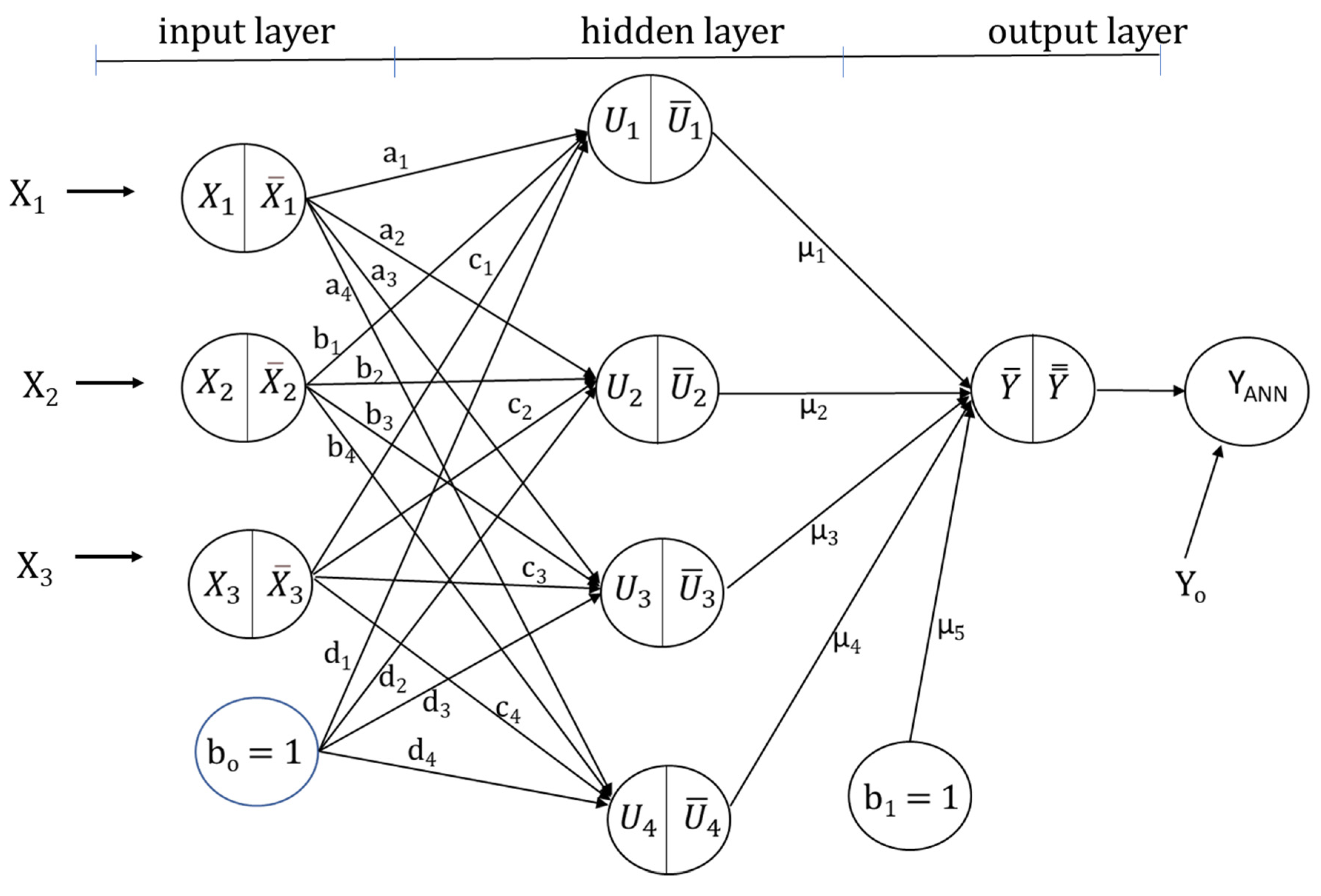
This study employed the feed-forward backpropagation neural network which is one of the most popular neural networks widely used due to its simplicity, accuracy, and efficiency in algorithm processing. It is often distinguished by one or more hidden layers in the ANN configuration which is normally followed by an output layer. Figure 1 shows the ANN configuration used in this study. The configuration consists of three layers which are the input, hidden, and output layers with three neurons constructed in the input layer to represent the value relating to the sediment and fluid characteristics. The neurons are also connected to four neurons in the hidden layer and transferred into one neuron in the output layer. This multiple layer configuration of neurons along with the nonlinear transfer function allows the learning process of the nonlinear relation between the input and output layers as indicated in the ANN configuration presented in Figure 1.

This study developed five ANN models, ANN1 to ANN5, with respect to the input and output parameters.

Table 2. Input and output parameters for ANN1 to ANN5.

Model	Input Parameters and Unit	Output Parameters and Unit
ANN1	X1 = d (mm), X2 = SF (non-dimensional parameter) and X3 = T (°C)	YANN = Ws (cm/s)
ANN2	X1 = log(d (mm)), X2 = SF and X3 = T (°C)	YANN = log (Ws), Ws (cm/s)
ANN3	X1 = SF and X2$=D_{*}$ (non-dimensional parameter)	YANN = log(Re)—non-dimensional parameter
ANN4	X1 = SF and X2$=\log \left(D_{*}\right)$	YANN = log(Re)—non-dimensional parameter
ANN5	X1 = SF and X2$=\log (D_{*}$)	YANN = log(CD)—non-dimensional parameter

shows the input and output parameters used in each ANN model. In the first model (ANN1), the original dataset was configured as the input parameters and these include X₁ = d is the nominal particle diameter in millimeter (mm), X₂ = T is the water temperature in °C, and X₃ = SF is the shape factor while the settling velocity, Y₀ = W_s (cm/s), was used as the target parameter in the output layer. Meanwhile, in the second model (ANN2), the logarithmic transformation was conducted for the particle diameter in the input layer, X₁ = log(d (mm)), and the log transformation of settling velocity as the output layer, Y₀ = log(W_s (cm/s)) while the water temperature and shape factor remain the same as in the first model. In the third to fifth models (ANN3 to ANN5), two non-dimensional parameters are used for the input and a non-dimensional parameter as the output. The input parameters for ANN3 are X₁ = SF and X₂ = $D_{*}$ and for ANN4 are X₁ = SF and X₂ = log$\left(D_{*}\right)$ while the output parameter for ANN3 and ANN4 is the same Y₀ = log(Re). The ANN5 uses the same input as the ANN4 with output Y₀ = log(C_D).

The second-order algorithm of Levenberg–Marquardt was adopted to avoid some drawbacks of the feed-forward algorithm in the local optima problem. This Levenberg–Marquardt method is also superior in reducing the learning time with less iteration compared to the traditional backpropagation algorithm, thereby, leading to an increase in the searching rate to search and obtain the weight and biases and achieve faster convergence with high precision.

2.3. Development of Explicit Equations

The explicit equations are developed based on the non-linear function of the neural network transfer function. This involved normalizing the input parameters, X_i, i = 1, 2, and 3 (number of input or node in input layer) in the initial step using their maximum (X_{i, max}) and minimum (X_{i, min}) values based on the following relation:

$$\overline{X_i}=2\left(X_i-X_{i,min}\right)/\left(X_{i,max}-X_{i,min}\right)-1$$

(5)

The normalized values ($\overline{X_i}$) and the bias with the value of unity (b_o = 1) are multiplied with their respective weight a_m, b_m, c_m, and d_m where m = 1, 2, 3, and 4. It is important to note that the number of weights of each input parameter is in line with the number of nodes in the hidden layer, such that a_m, b_m, and c_m represent the weight of each input node, respectively, while the index, m, represents the node number in the hidden layer and d_m indicates the weighting factor of the bias node for each hidden layer node ‘m’. Moreover, the input value for nodes in the hidden layer is provided by multiplying the normalized input and the product was summed to determine the neuron’s value in the hidden layer input, U_m, through the linear relationship presented in Equation (6).

$$U_m=a_m\overline{X_1}+b_m\overline{X_2}+c_m\overline{X_3}+d_m$$

(6)

The input in the hidden layer nodes is later transferred using the non-linear transferred function of a hyperbolic tangent to produce the final value in each hidden layer neuron, ${\overline{U}}_m$. Finally, each value of ${\overline{U}}_m$ is multiplied with the respective weight, μ_m, such that the index ‘m’ represents the number node of in the hidden layer and additional bias node. The values obtained are summed to provide the input value for the output node based on the following equation.

$$\overline{Y}={\mu }_1 tanh\left({\overline{U}}_1\right)+{\mu }_2 tanh \left({\overline{U}}_2\right)+{\mu }_3 tanh\left({\overline{U}}_3\right)+{\mu }_4 tanh\left({\overline{U}}_4\right)+{\mu }_5$$

(7)

The linear transformation is used to provide the normalized output value, $\stackrel{=}{Y}$, to ensure $\overline{Y}=\stackrel{=}{Y}$ while the final output Y_ANN is obtained after $\stackrel{=}{Y}$ is denormalized to produce the following explicit Equation (8).

$$Y_{ANN}={\displaystyle \sum }_{k=1}^4{A}_{k}tanh\left(a_k{\overline{X}}_1+b_k{\overline{X}}_2+c_k{\overline{X}}_3+d_k\right)+B$$

(8)

where Y_ANN is the predicted value relating to W_s, Re or C_D and A_k and B are coefficients that depend on the weights a_k, b_k, c_k, and d_k where k = 1, 2, 3, and 4. These weight coefficients are obtained through a training process in the ANN model with the objective function of minimizing the error of each output value based on the following equation:

$$min E\left(Y_{ANN}\right)= min{\displaystyle \sum }_{i=1}^N{\left(Y_{ANN,i}-Y_{0,i}\right)}^2$$

(9)

where Y₀ is the ANN target value relating to W_s, log(W_s), log(Re), and log(C_D) for ANN1, ANN2, ANN3 & ANN4, and ANN5, respectively, and N is the amount of data. The application of a simple configuration of the ANN model led to an additional optimization process after the weight coefficients are produced from MATLAB. This involved developing an additional ANN algorithm using the Excel spreadsheets to change $\stackrel{=}{Y}$ in the form of the original data set to produce the final output value Y_ANN and also to develop the explicit equation defined in equation (8) towards improving the model. The optimization is conducted using the iterative process with the Generalized Reduced Gradient Non-Linear (GRG Nonlinear) method.

2.4. Comparison with Existing Formulas

The proposed equations, ANN1 to ANN5, will be compared with three existing formulas for estimating the settling velocity of sediment particles. The first formula is developed by Jiménez and Madsen [21] to predict setting velocity W_s. They built the equation to determine W_s from the previous study by Dietrich [17]. They proposed an equation to estimate W_s for sediment particles with a given shape factor, roundness parameter, and diameter using Equation (10):

$$W_s=\frac{\sqrt{\left({\rho }_s/{\rho }_f-1\right)gd}}{C+\frac{D}{S_{*}}}$$

(10)

In which,

$$S_{*}=\frac{d}{4\vartheta }\sqrt{\left({\rho }_s/{\rho }_f-1\right)gd}$$

(11)

where C and D depend on shape factor (SF) and particle roundness (P). They provided relationship charts between the values of C and D concerning SF and P. For natural sediment particles, the values for SF = 0.7 and P = 3.5, and the values for C and D are 0.954 and 5.12. Wu and Wang [11] developed the second equation to determine W_s using the following Equation (12)

$$W_s=\frac{M_w\vartheta }{N_{w}d} {\left[ \sqrt{{\left(\frac{4N_w}{3{\left(M_w\right)}^2}{D}_{*}^3\right)}^{\frac{1}{n}}+\frac{1}{4}} -\frac{1}{2}\right]}^n$$

(12)

where M_w, N_w and n are coefficients obtained from the calibration results, namely M_w = 53 5e^−0.655SF, N_w = 5.65e^−2.5SF, and n = 0.7 + 0.9 SF. Camenen [23] developed an equation to determine the value of W_s by considering the shape factor SF and roundness (P) using the following equation:

$$W_s=\frac{\vartheta }{d}{\left[\sqrt{\frac{1}{4}{\left(\frac{A}{B}\right)}^{\frac{2}{n}}+{\left(\frac{4}{3}\frac{D_{*}^3}{B}\right)}^{\frac{1}{n}}}-\frac{1}{2}{\left(\frac{A}{B}\right)}^{\frac{1}{n}}\right]}^n$$

(13)

where A, B, and n are calibration coefficients depending on the shape factor SF, and roundness (P):

$$A=a_1+a_2{\left[1-sin\left(\frac{\pi }{2}SF\right)\right]}^{a_3}$$

(14)

$$B=b_1+b_2{\left[1-sin\left(\frac{\pi }{2}SF\right)\right]}^{b_3}$$

(15)

$$n= n_1{\left[sin\left(\frac{\pi }{2}SF\right)\right]}^{n_2}$$

(16)

where a₁ = 24, b₁ = 0.39 + 0.22(6 − P), n₁ = 1.2 + 0.12P, a₂ = 100, b₂ = 20, n₂ = 0.47, a₃ = 2.1 + 0.06P and b₃ =1.75 + 0.35P. For a particle roundness (P = 3.5): b₁ = 0.94, n₁ = 1.65, a₃ = 2.31 and b₃ = 2.975. The statistical measure of these three existing equations will be calculated and used as the comparison with the developed explicit equation.

2.5. Statistical Performance

The ANN1 to ANN5 performance is evaluated based on four statistical measures which include:

• Coefficient of determination, R², between the W_sp and W_se, where W_sp is the predicted settling velocity and W_se are the data obtained from digitizing the Interagency Committee’s chart and measurement data compiled from several sources for each input parameter of sediment and fluid characteristic. The coefficient of determination ranges from 0 to 1 defined as:

$$R^2=\frac{{{\displaystyle \sum }}_{i=1}^N\left(W_{se,i}-{\overline{W}}_{se}\right)\left(W_{sp,i}-{\overline{W}}_{sp}\right)}{\sqrt{{{\displaystyle \sum }}_{i=1}^N{\left(W_{se,i}-{\overline{W}}_{se}\right)}^2}\sqrt{{{\displaystyle \sum }}_{i=1}^N{\left(W_{sp,i}-{\overline{W}}_{sp}\right)}^2}}$$

(17)

where ${\overline{W}}_{se}$ and ${\overline{W}}_{sp}$ are mean digitized or measured and predicted data, respectively, and N is the amount of data.

2.

Mean absolute relative error, MRE, which is defined as:

$$MRE=\frac{1}{N}{\displaystyle \sum }_{i=1}^N\left|\frac{W_{se,i}-W_{sp,i}}{W_{se,i}}\right|\times 100\%$$

(18)

3.

Maximum absolute relative error, MAXRE, which is defined as:

$$MAXRE=max {\displaystyle \sum }_{i=1}^N\left|\frac{W_{se,i}-W_{sp,i} }{W_{se,i}}\right|\times 100\%$$

(19)

4.

Root Mean Square Error. (RMSE). RMSE is a standard way to estimate the error of an equation in estimating real values-responses [3]. RMSE is defined by Equation (20)

$$RMSE=\sqrt{{\displaystyle \sum }_{i=1}^N\frac{{\left(W_{se,i}-W_{sp,i}\right)}^2}{N}}$$

(20)

3. Results and Discussion

The training conducted using the MATLAB program produced weights coefficients a, b, c, d, and μ for five ANN models, and these weight values were used as the initial values for further optimizations in the MS Excel program developed by the author. These optimizations were conducted using the objective function of minimizing MRE as defined in Equation (18) to further minimize the relative error of the predicted settling velocity as indicated by the coefficients produced for the ANN models in

Table 3. Coefficient of Equation (8) for ANN1 model.

	Coefficient
k	ak	bk	ck	dk	Ak	B
1	0.296	0.0713	0.1162	1.6124	43.8976	−98.0281
2	−6.1369	−3.661	0.996	1.3414	3.2274
3	−0.3883	−0.1107	−0.1664	1.039	−74.0032
4	1.4203	−0.0537	−0.0894	2.6377	146.6105

,

Table 4. Coefficient of Equation (8) for ANN2 model.

	Coefficient
k	ak	bk	ck	dk	Ak	B
1	1.0431	1.2349	−0.0188	2.0878	0.0623	−0.5864
2	−0.2999	−1.6478	1.8649	1.5139	0.0123
3	−0.7134	0.0237	−0.2138	0.7840	−0.5145
4	0.8745	0.0731	−0.0041	1.0787	2.2831

,

Table 5. Coefficient of Equation (8) for ANN3 model.

	Coefficient
k	ak	bk	ck	dk	Ak	B
1	−0.0039	−0.0152	0	0.1779	−28.7443	−43.2153
2	−0.014	11.4145	0	12.8343	13.7859
3	0.0067	57.9223	0	59.8398	22.6845
4	0.0232	−1.8331	0	−3.2811	−15.0682

,

Table 6. Coefficient of Equation (8) for ANN4 model.

	Coefficient
k	ak	bk	ck	dk	Ak	B
1	−0.0305	0.8205	0	0.9759	2.9174	37.2271
2	−1.3304	−3.195	0	−0.9563	0.0191
3	−26.6184	16.1434	0	−4.3576	−0.0086
4	−0.0059	−0.0768	0	1.0946	−47.1924

and

Table 7. Coefficient of Equation (8) for ANN5 model.

	Coefficient
k	ak	bk	ck	dk	Ak	B
1	0.2694	−1.2492	0	−1.2904	2.2816	2.6739
2	−4.7911	2.3532	0	2.0994	0.1445
3	−8.1959	−4.3167	0	−1.1346	0.1038
4	−1.0957	−2.2051	0	−2.2642	0.4561

. Thus, the explicit ANN1 to determine the settling velocity is Equation (8) with coefficients a_k, b_k, c_k, d_k, A_k, and B in Table 3 with normalized parameters defined by Equation (21).

$${\overline{X}}_1=0.2012d-1.0121,{\overline{X}}_2=0.05T-1,{\overline{X}}_3=5SF-3.5,and{Y}_{ANN}=W_s$$

(21)

where d (mm), T (°C), SF (-), W_s (cm/s).

The explicit ANN2 uses Equation (8) with coefficients in Table 4 and uses normalized parameters in Equation (22).

$${\overline{X}}_1=0.90 log\left(d\right)+0.09971, {\overline{X}}_2=0.05 T-1, {\overline{X}}_3=5SF-3.5, and Y_{ANN}=log(W_s)$$

(22)

where d (mm), T (°C), SF (-), W_s (cm/s).

The explicit ANN3 uses Equation (8) with coefficients in Table 5 and uses normalized parameters in Equation (23).

$${\overline{X}}_1=5SF-3.5, {\overline{X}}_2=0.00751D_{*}-1.0077, {\overline{X}}_3=0, and Y_{ANN}=log\left(Re\right)$$

(23)

The explicit ANN4 uses Equation (8) with coefficients in Table 6 and uses normalized parameters in Equation (24).

$${\overline{X}}_1=5SF-3.5, {\overline{X}}_2=0.82864log\left(D_{*}\right)-1.0083, {\overline{X}}_3=0, and Y_{ANN}=log\left(Re\right)$$

(24)

The explicit ANN5 uses Equation (8) with coefficients in Table 7 and uses normalized parameters in Equation (25).

$${\overline{X}}_1=5SF-3.5, {\overline{X}}_2=0.82864log\left(D_{*}\right)-1.0083, {\overline{X}}_3=0, and Y_{ANN}=log\left(C_D\right)$$

(25)

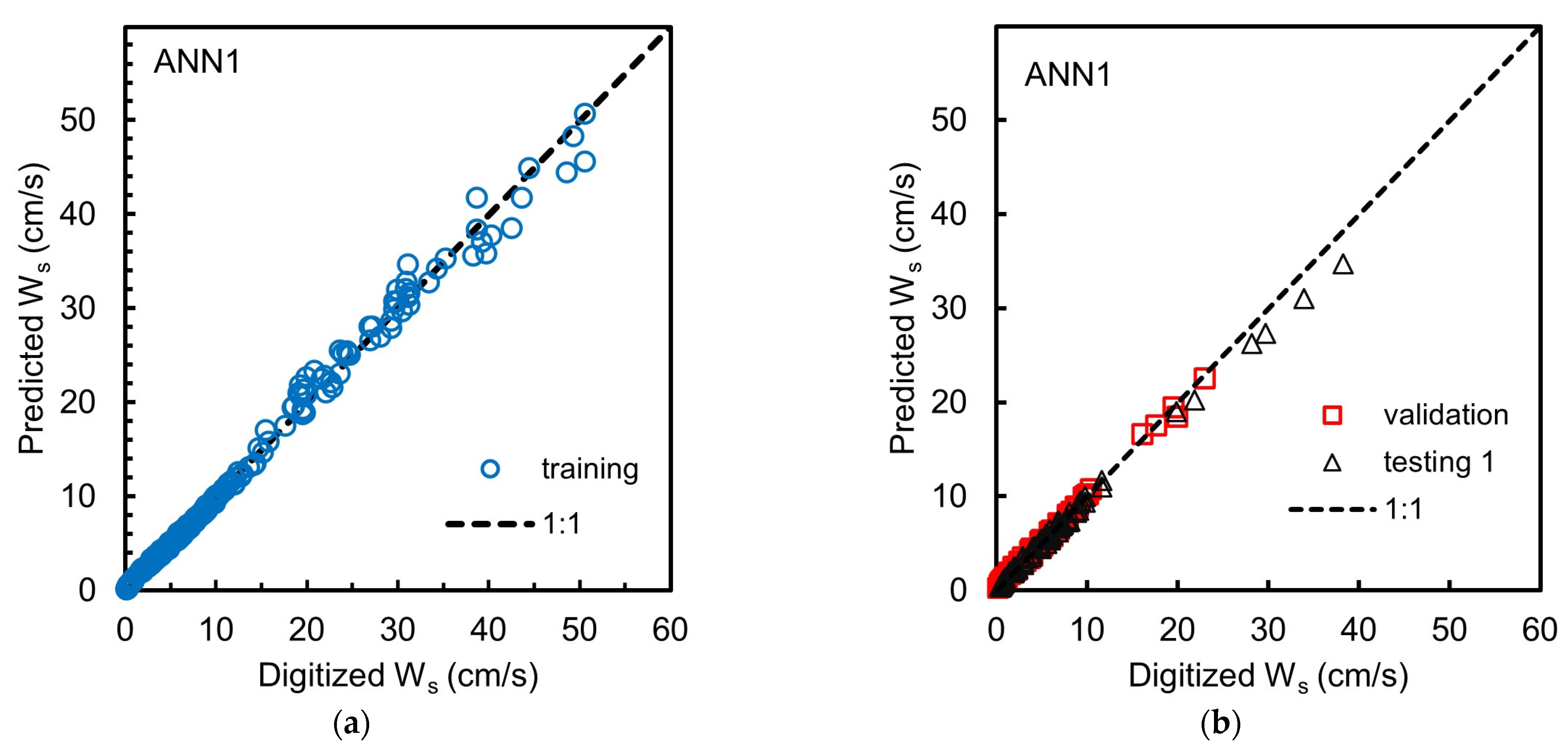
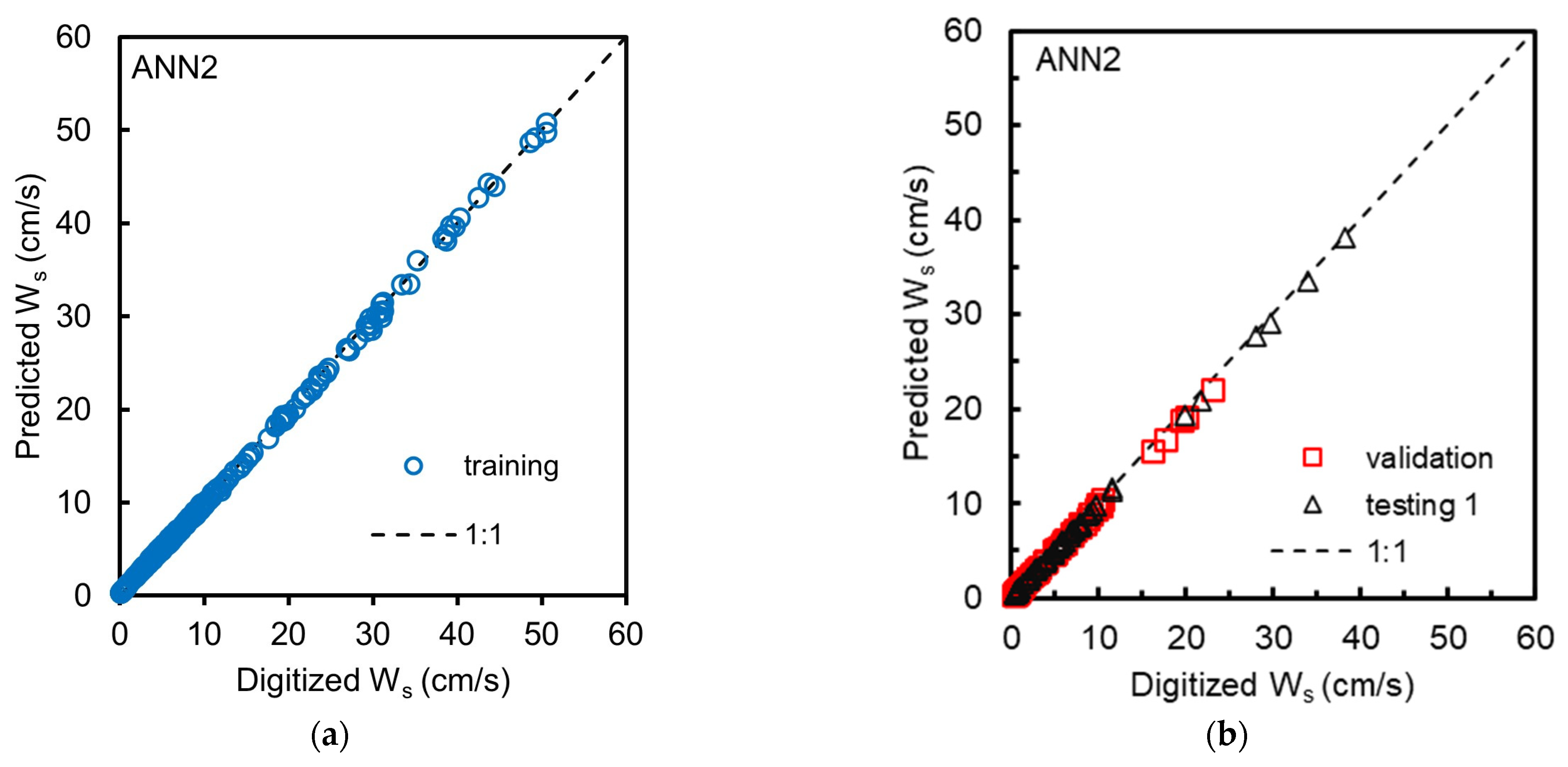
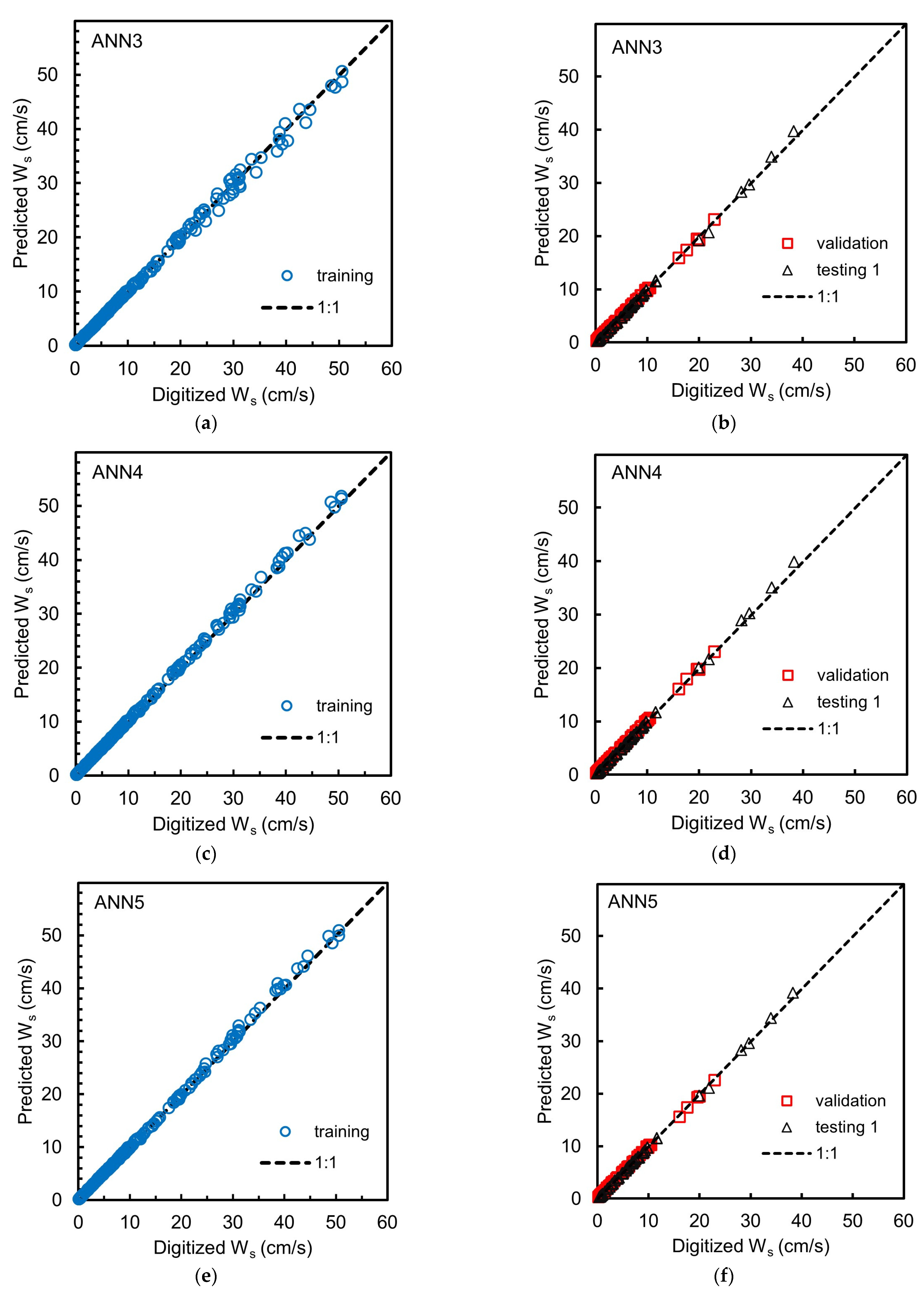
Figure 2, Figure 3 and Figure 4 show the scatter plot between the predicted settling velocity and the digitized data from the Interagency Committee’s charts for training, validation, and testing 1 for the ANN1 to ANN5 models, respectively. Moreover, the statistical measures of the simulation results for the training, validation, and testing 1 of the five ANN models are provided in

Table 8. Statistical measures for ANN1 to ANN5.

Model		MRE	MAXRE	RMSE	R2
ANN1	Training	7.88	80.92	0.76	0.9951
	Validation	9.41	44.47	0.30	0.9968
	Testing 1	10.20	47.17	0.68	0.9973
ANN2	Training	2.71	6.91	0.32	0.9996
	Validation	2.17	5.57	0.23	0.9996
	Testing 1	2.37	7.96	0.18	0.9996
ANN3	Training	2.16	8.31	0.47	0.9996
	Validation	2.48	8.04	0.12	0.9995
	Testing 1	1.89	5.06	0.26	0.9990
ANN4	Training	1.24	5.55	0.23	0.9996
	Validation	1.39	3.97	0.09	0.9998
	Testing 1	1.57	4.10	0.19	0.9996
ANN5	Training	1.52	5.55	0.29	0.9994
	Validation	1.69	4.74	0.14	0.9997
	Testing 1	1.35	3.84	0.15	0.9996

.

The results show that the coefficient of determination (R²) for the ANN1 to ANN5 models is excellent, as indicated by the values estimated to be more than 0.995. The simulation of the ANN1 produced MRE of 7.88%, 9.41%, and 10.20% for training, validation, and testing 1, respectively. The MAXRE values produced by ANN1 are 80.92%, 44.47%, and 47.17% for training, validation, and testing 1, respectively. However, the ANN2 and ANN3 produced more satisfactory results in terms of MRE and MAXRE, with the MRE between 1.89% and 2.71% in training, validation, and testing 1, respectively, while the MAXRE is between 5.06% and 8.31% in the training, validation and testing 1, respectively. Moreover, the ANN4 and ANN5 produced very satisfactory results in terms of MRE and MAXRE, with the MRE in the range of 1.24–1.69 in training, validation, and testing 1, respectively, while the MAXRE in the range of 3.84% to 5.55% in training, validation and testing 1, respectively.

To find out the contribution of the error to ANN1, we provide scattering plot for results of the ANN1 and ANN2 models for W_s values lower than 10 cm/s, as seen in Figure 5. It was discovered that the prediction of the settling velocity using the ANN1 (see Figure 5) provided inaccurate results for W_s smaller than 10 cm/s which is related to grain sizes smaller than 1 mm. These errors may be because the Interagency Committee’s charts were constructed for data with Re > 3, and the curves were extended for Re < 3 using Stokes’ law assumptions [1,11]. However, the ANN2 produced very satisfactory results for all particle sizes (d), Safe Factor (SF), and water temperature (T) under consideration.

The coefficients A₂ and A₃ of the ANN 4 equation in Table 6 have relatively small values, so their effect on the overall function value is small. By removing the coefficients A₂ and A₃ and applying the optimization technique, new coefficients a, b and A₁, A₄, and B are determined, resulting in a simplified form of explicit Equation (8) for ANN4.

$$Log\left(Re\right)=2.7001 tanh\left(-0.0329{\eta }_1+0.8483{\eta }_2+0.9665\right)-45.2316 tanh\left(-0.0057{\eta }_1-0.0756{\eta }_2+1.0567\right)+35.1902$$

(26)

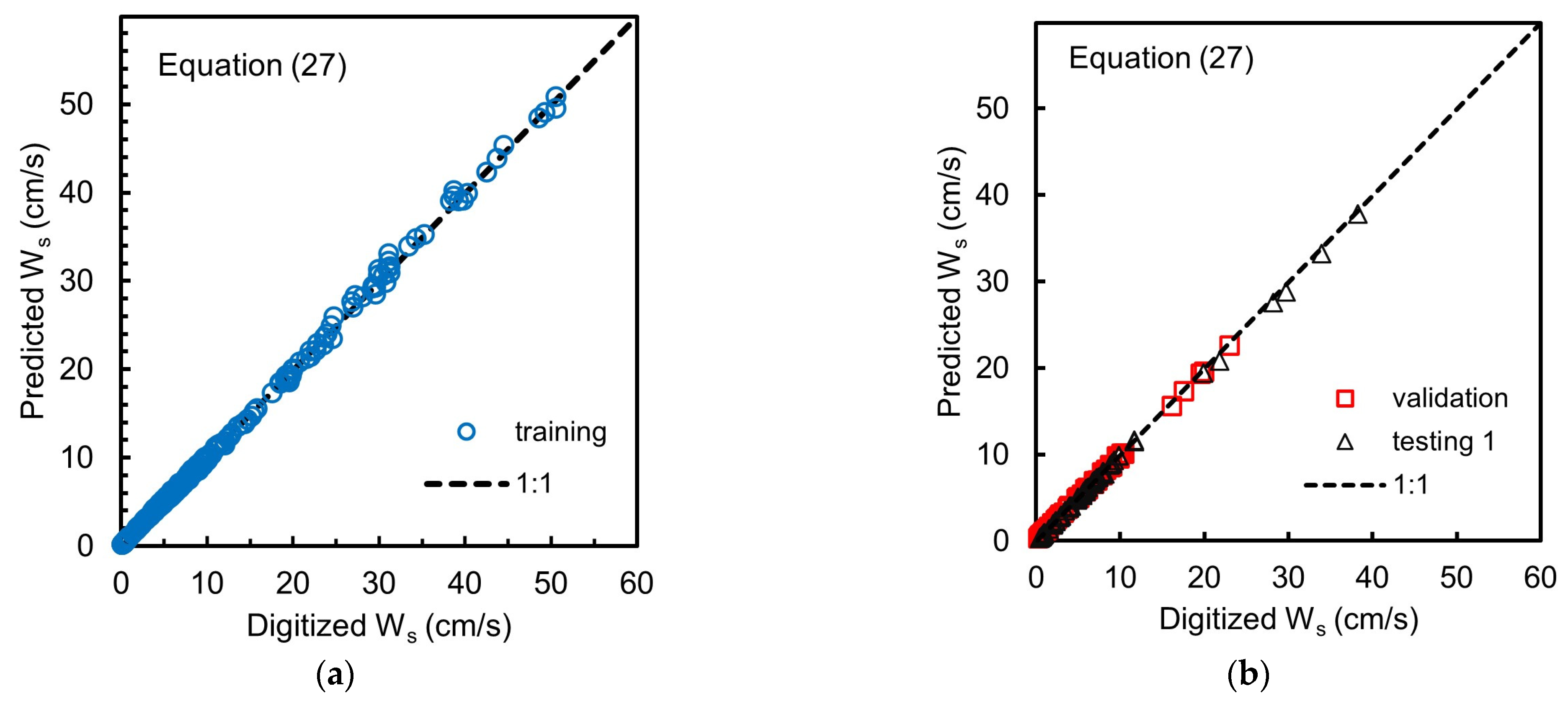
where ${\eta }_1=5SF-3.5 and {\eta }_2=0.82864log\left(D_{*}\right)-1.0083.$ The coefficients A₂ and A₃ for ANN5 are also relatively small. By performing the same procedure to obtain the simplification of the ANN 4 equation, the simplified form of Equation (8) for ANN 5 is:

$$Log(C_D)=2.148 tanh\left(0.0824{\eta }_1-1.3963{\eta }_2-1.1600\right)+0.2902 tanh\left(-0.8174{\eta }_1+0.1532{\eta }_2-0.0501\right)+2.1129$$

(27)

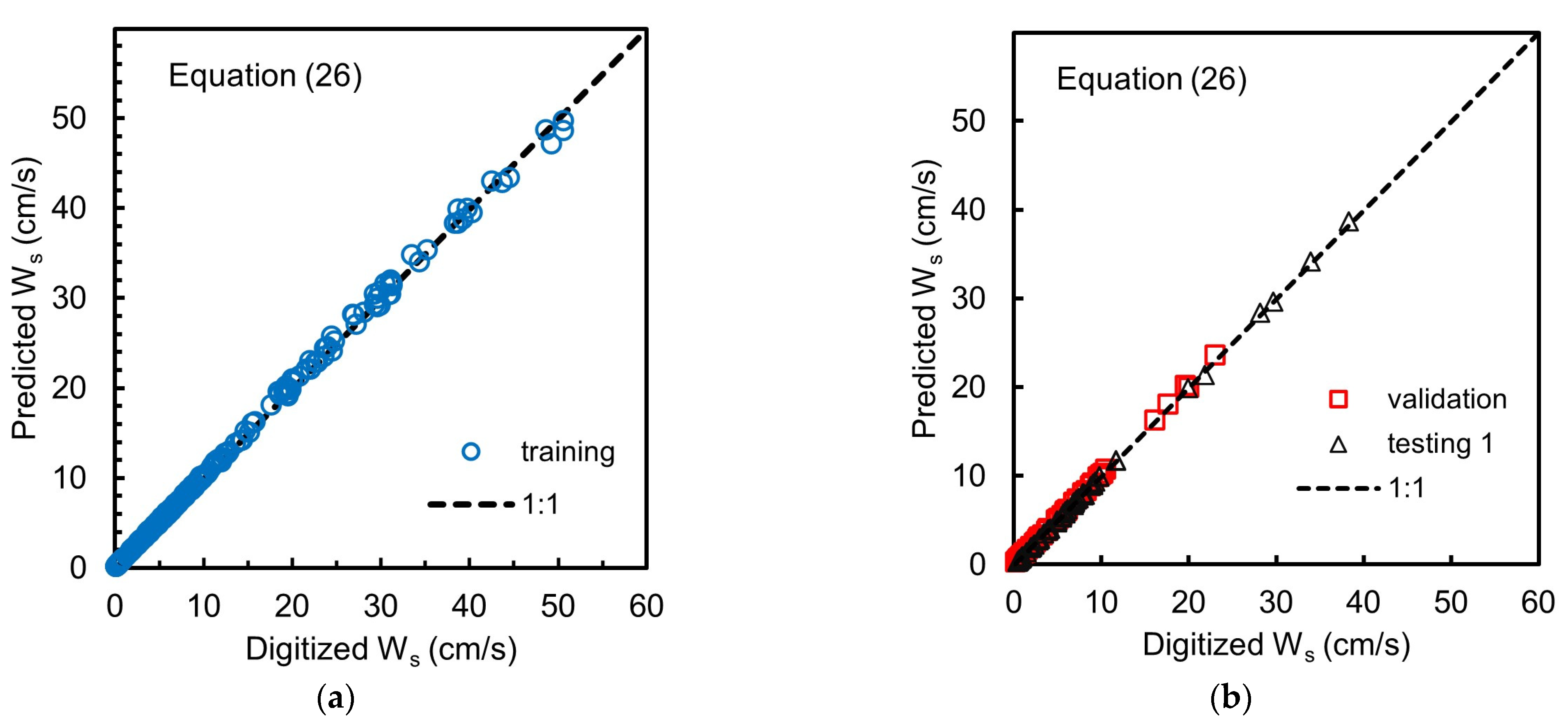
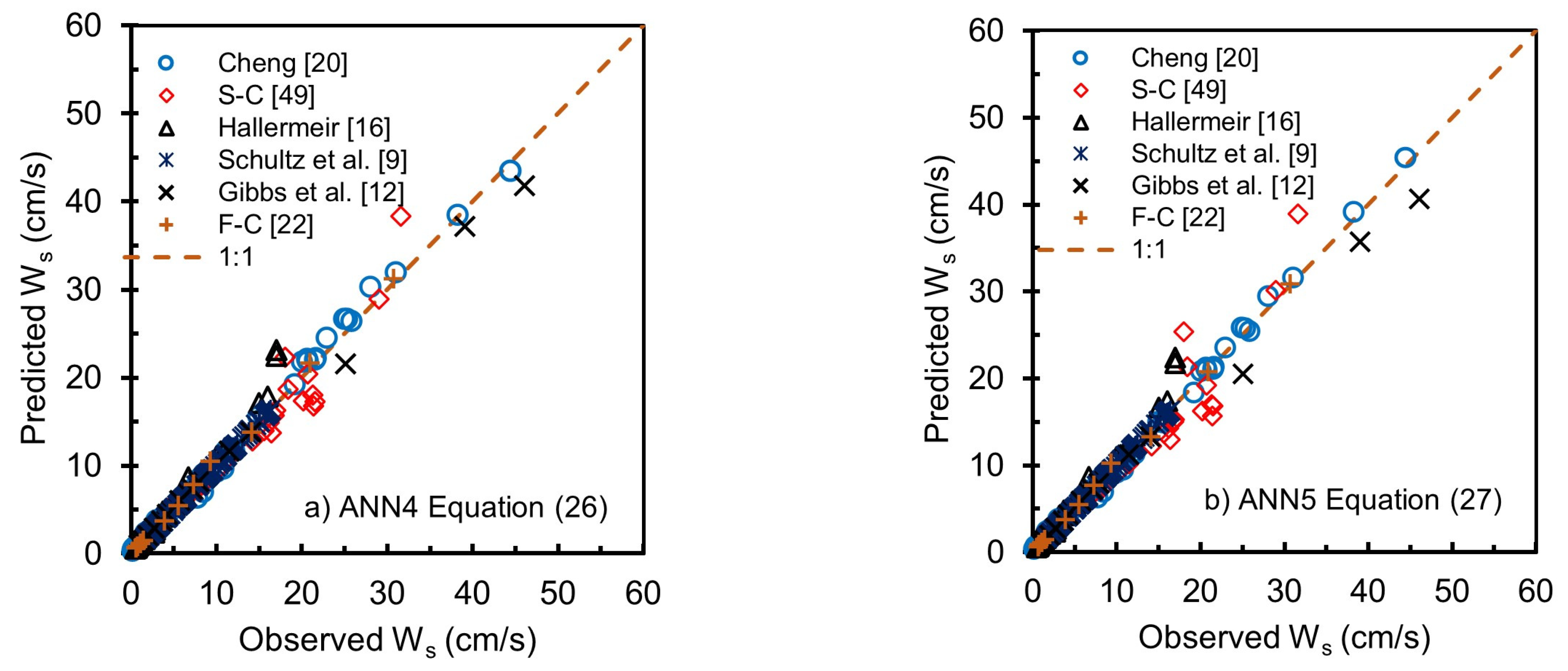
where${\eta }_1=5SF-3.5 and {\eta }_2=0.82864log\left(D_{*}\right)-1.0083.$ Statistical measures of the simulation results for the training, validation, and testing 1 of the simplified ANN4 Equation (26) and simplified ANN5 Equation (27) are given in

Table 9. Statistical measures for ANN4 Equation (26) and ANN5 Equation (27).

	Simplified ANN4, Equation (26)				Simplified ANN5, Equation (27)
Simulation	MRE	MAXRE	RMSE	R2	MRE	MAXRE	RMSE	R2
	(%)	(%)			(%)	(%)
Training	2.55	8.38	0.34	0.9991	2.15	6.01	0.31	0.9992
Validation	2.58	6.10	0.12	0.9998	1.81	5.24	0.18	1.00
Testing 1	2.16	4.87	0.14	0.9998	2.11	6.40	0.20	0.9996

. Figure 6 and Figure 7 show the scatter plot between the predicted settling velocity and the digitized data from the Interagency Committee’s charts for training, validation, and testing 1 for the simplified ANN4 Equation (26) and the simplified ANN5 Equation (27), respectively.

Table 10. Statistical measures for ANN1 to ANN5 as well as existing equations and ANN4 Equation (26) and ANN5 Equation (27) for testing 2.

Formula	MRE (%)	MAXRE (%)	RMSE	R2
ANN1	10.84	68.86	1.16	0.9785
ANN2	9.65	56.01	1.24	0.9762
ANN3	9.15	54.24	1.18	0.9778
ANN4	9.17	55.26	1.21	0.9763
ANN5	10.78	100.51	1.41	0.9680
* Jimenez and Madsen [21]	11.45	64.98	1.56	0.9639
* Wu and Wang [11]	9.21	56.22	1.23	0.9759
* Camenen [23]	11.54	74.70	1.66	0.9582
Simplified ANN4, Equation (26)	9.73	58.49	1.19	0.9777
Simplified ANN5, Equation (27)	9.31	60.24	1.35	0.9706

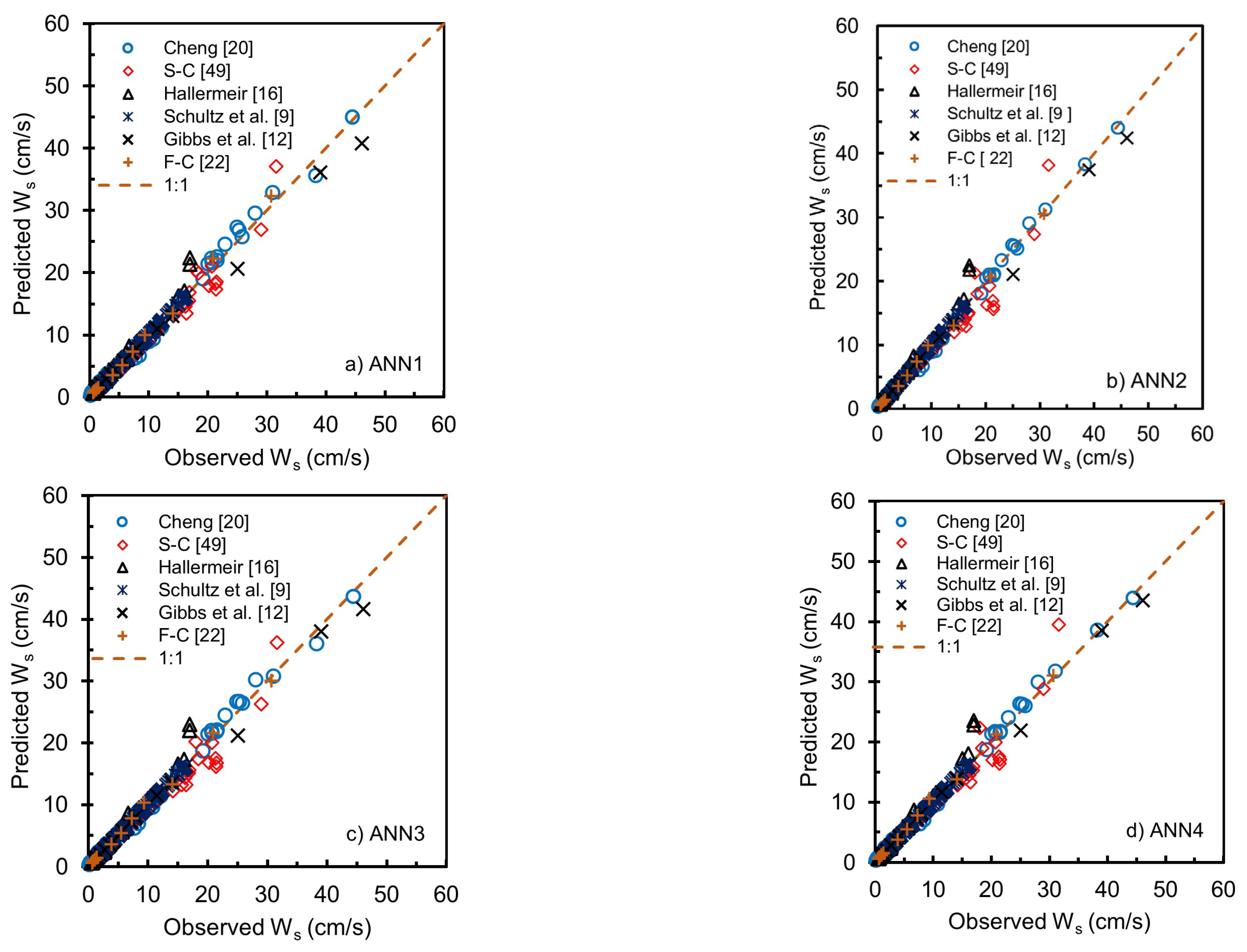
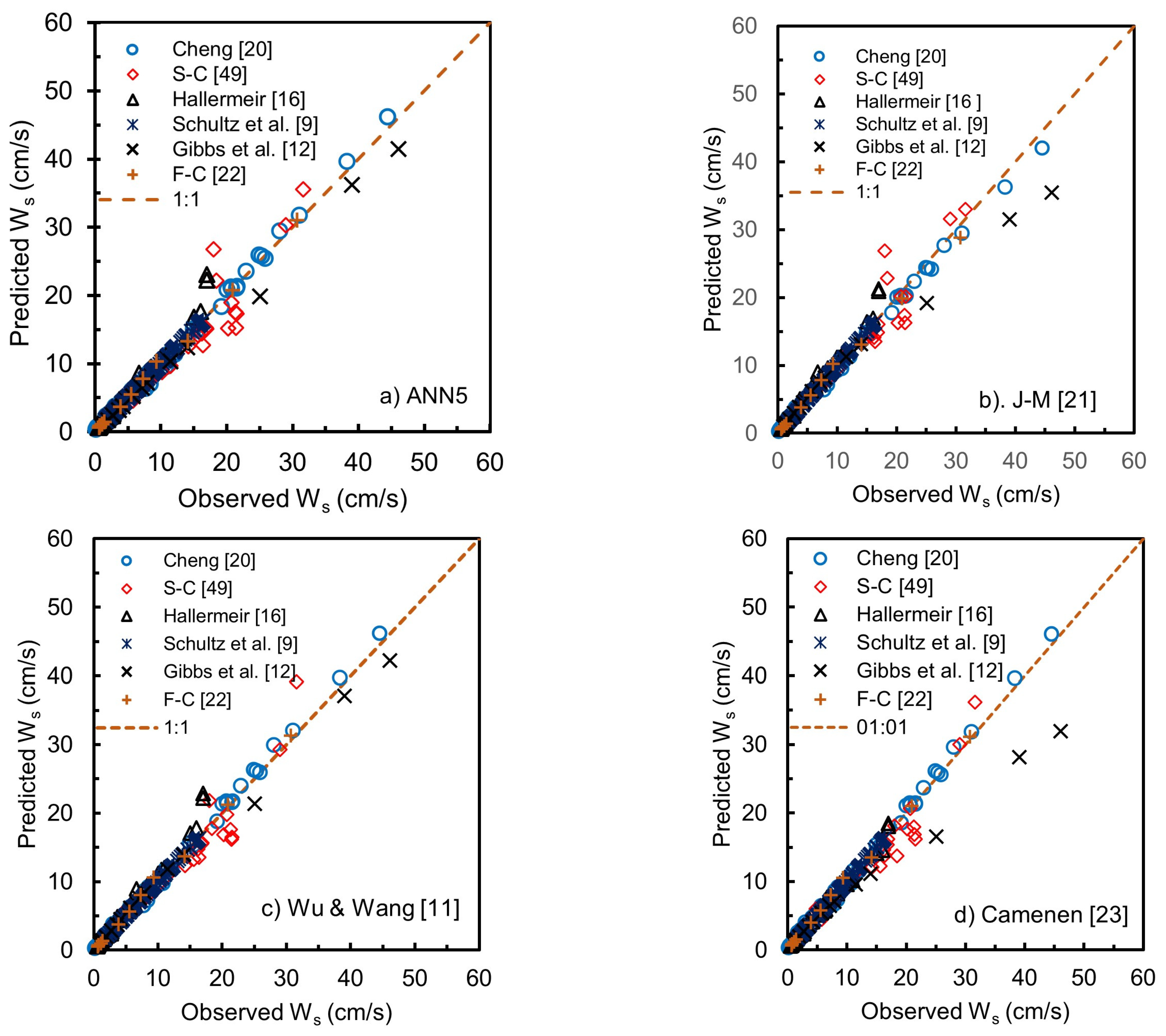
* Existing formulas compared to this study.

presents the statistical values of the results of testing 2 for the five models, ANN1 to ANN5, as well as the three existing equations reviewed, Jiminez and Madsen [21], Wu and Wang [11], and Camenen [23], and also the simplified ANN4 Equation (26) and simplified ANN 5 Equation (27), respectively. Plotting between W_s predictions and data is given in Figure 8, Figure 9 and Figure 10. As in the previous test results, ANN3 and ANN4 give slightly more accurate results than other proposed ANN. The MRE, MAXRE, and RMSE values of results of ANN3 and ANN4 are lower than other ANNs. The simulation results also show that ANN2 and the formula of Wu and Wang [11] provide MRE, MAXRE, RMSE, and R² values close to each other. It is not surprising because the Wu-Wang formula [11] was also developed using the Interagency Committee’s charts as a reference. Shankar et al. [50] also conclude that the Wu-Wang model predicts the settling velocity of sediment particles better than the 14 existing models reviewed in their comparison study. Through visual observations in Figure 9, the results of plotting the models of Jeminez-Madsen [21] and Camenen [23], there are quite large deviations in some data with W_s between 40 to 50 cm/s. Surprisingly, the simplified model of ANN4 Equation (26) and ANN5 Equation (27) produce statistical measures nearly the same as its full equation (Figure 8d and Figure 9e).

The above results indicate that the simplified ANN4 Equation (26) and simplified ANN5 Equation (27) can potentially be used to predict the settling velocity of natural sediments, especially for those sediment quartz with diameters between 0.05 mm and 10 mm in water having temperatures between 0 °C and 40 °C and the shape factor ranging between 0.5 and 0.95 with reasonable accuracy.

4. Application of Explicit Equations

The following are examples of using the ANN formula Equation (8). Examples are given for ANN1 and ANN2 formulas. The data are taken from a sample test result by Smith and Cheung [49] with grain diameter d = 0.59 mm, water temperature T = 20 °C, particle safe factor SF = 0.62 and measured settling velocity W_se = 7.3 cm/s. For the application of the formula ANN1, settling velocity W_sp can be estimated using Equation (8) with coefficients and normalized parameters in Table 3. The detailed calculation can be described as follows:

Normalized parameters from Equation (21),

$$\begin{gathered} {\overline{X}}_1=(0.2012\times 0.59)-1.0221=-0.89336 \\ {\overline{X}}_2=(0.05\times 20)-1=0 \\ {\overline{X}}_3=(5\times 0.62)-3.5=-0.4 \end{gathered}$$

Predict the settling velocity using Equation (8) with coefficients (a_k, b_k, c_k, d_k, A_k and B) on Table 3, elaborate Equation (8) for k = 1,2,3 and 4,

$$W_s=W_{s_{,k=1}}+W_{s{,}_{k=2}}+W_{s{,}_{k=3}}+W_{s{,}_{k=4}}+B$$

(28)

$$W_{s_{,k=1}}=43.8976\times \mathit{tanh}\left(\left(0.296\times -0.89336\right)+\left(0.0713\times 0\right)+\left(0.1162\times -0.4\right)+1.6124\right)$$

$$W_{s_{,k=2}}=3.2274\times \mathit{tanh}\left(\left(-6.1369\times -0.89336\right)-\left(3.661\times 0 \right)+\left(0.996 \times -0.4\right)+1.3414\right)$$

$$W_{s_{,k=3}}=-74.0032\times \mathit{tanh}(\left(-0.3883\times -0.89336)-\left(0.1107\times 0\right)-\left(0.1664\times -0.4\right)+1.039\right)$$

$$W_{s_{,k=4}}=146.6105\times tanh (\left(1.4203\times -0.89336)-\left(0.0537\times 0\right)-\left(0.0894\times -0.4\right)+2.6377\right)$$

$$B=-98.0281$$

Thus, we obtain $W_s=6.67\mathrm{cm}/\mathrm{s}$.

Based on the explicit equation developed from the ANN1 model, the result shows the absolute relative error = abs((7.3 − 6.67)/7.3) = 8.61%.

For the application of Formula ANN2, the predicted settling velocity W_sp can be estimated using Equation (8) with coefficients in Table 4 and normalized parameters from Equation (22). The detailed calculation can be described as follows:

Normalized parameter

$$\begin{gathered} {\overline{X}}_1=(0.90\times log(0.59\left)\right)+0.09971=-0.106568 \\ {\overline{X}}_2=(0.05\times 20)-1=0 \\ {\overline{X}}_3=(5\times 0.62)-3.5=-0.4 \end{gathered}$$

Predict the settling velocity:

$$Log\left(W_s\right)=W_{s_{,k=1}}+W_{s{,}_{k=2}}+W_{s{,}_{k=3}}+W_{s{,}_{k=4}}+B$$

(29)

$$W_{s_{,k=1}}=0.0623\times \mathit{tanh}\left(\left(1.0431\times -0.106568\right)+\left(1.2349\times 0\right)-\left(0.0188\times -0.4\right)+2.0878\right)$$

$$W_{s_{,k=2}}=0.0123\times \mathit{tanh}\left(\left(-0.2999\times -0.106568\right)-\left(1.6478\times 0\right)+\left(1.8649\times -0.4\right)+1.5139\right)$$

$$W_{s_{,k=3}}=-0.5145\times \mathit{tanh}\left(\left(-0.7134\times -0.106568\right)+\left(0.0237\times 0\right)-\left( 0.2138\times -0.4\right)+0.784\right)$$

$$W_{s_{,k=4}}=2.2831\times \mathit{tanh}\left(\left(0.8745\times -0.106568\right)+\left(0.0731\times 0\right)-\left(0.0041\times -0.4\right)+2.2831\right)$$

$$B=-0.5864$$

$$\mathrm{Thus},\mathrm{we}\mathrm{obtain}log(W_s)=0.832508\mathrm{and}{W}_s={10}^{0.832508}=6.80\mathrm{cm}/\mathrm{s}$$

The explicit formula developed from model ANN2 produces the absolute relative error = abs((7.3−6.8)/7.3) = 6.84%. The relatively low relative error is shown for both formulas.

5. Conclusions

This study develops five explicit ANN formulas, ANN1 to ANN5, to predict the settling velocity of sediment particles with variations in grain size, particle shape factor, and water temperature using the ANN procedure. The process involved in developing the ANN models consists of using the data obtained from digitizing the Interagency Committee’s charts and additional settling velocity measurement data from several sources. The proposed ANN formulas explicitly express the Interagency Committee’s charts. The proposed ANN models are compared with three existing equations for predicting settling velocity, including the equation of Jiménez and Madsen [21], Wu and Wang [11], and Camenen [23], to evaluate their performances. The simulation results show that all ANN models, ANN1 to ANN5, produce accurate results. However, the ANN using non-dimensional inputs and outputs, such as ANN3, ANN4, and ANN5 have very satisfactory results. The results show the quality of ANN2 models is very close to that proposed by Wu and Wang [11]. Moreover, the equations of ANN4 and ANN5 can be simplified by omitting the two insignificant coefficients A₂ and A₃ giving the simpler equation of ANN4, Equation (26) and the simple equation of ANN5, Equation (27). Both Equation (26) and (27) produce very satisfactory results, nearly the same as in their full Equation (8). Thus, Equations (26) and (27) have a high potential to be used in predicting the settling velocity of particle sediment for quartz with a density around 2650 kg/m³, especially for diameters between 0.05 mm and 10 mm in water with temperatures between 0 °C and 40 °C and the shape factor of grains ranging between 0.5 and 0.95.

This study proposes an explicit expression of an ANN multilayer perceptron (MLP) consisting of three layers, input, hidden, and output layers. The output layer consists of a single node. The straightforward equation is defined by Equation (8). Equation (8) is a series of hyperbolic tangent functions with the sequence number according to the number of nodes in the hidden layer. Each hyperbolic tangent part contains coefficients with the number of coefficients equal to the number of input parameters. The MATLAB software can determine the series coefficient and the initial value for the optimization to obtain the best coefficients. Removing small values of series coefficients of hyperbolic tangent and re-optimizing to determine the new series and weight coefficients can simplify Equation (8). Equation (8) is a general form of explicit expression of an ANN multilayer perceptron with three layers and a single output node. Equation (8) can be applied to other cases using the same ANN approach to find the relationship between input parameters and outputs. For example, the explicit ANN Equation (8) will be helpful because it can also be applied to obtain sediment parameters that must be obtained through many graphic interpolations widely found in sediment transport computation.

It is noted that the ANN model proposed in this study uses data (sediment, fluid properties, and settling velocity), generally from the results of laboratory experiments obtained from the literature. Therefore, the proposed ANN model applies to hydrodynamic and fluid conditions during the investigation. The settling velocity experiment was generally carried out under stationary flow conditions. However, the settling process in the field is very complex, with many influencing factors, such as flow velocity, turbulence, sediment concentration, salinity, viscosity, fluid temperature, etc. Therefore, the development of advanced methods and tools that can measure the settling velocity in the field along with the hydrodynamic and fluid conditions during measurement is a challenge. Measurements are carried out under several hydrodynamic and fluid conditions and locations. Using data from field measurements (big data), we can build a fall velocity equation that is more in line with field conditions as a function of hydrodynamic and fluid parameters by using ANN in the explicit form of Equation (8). The use of an ANN is very suitable because it can produce an input-output relationship for a nonlinear and complex process, such as a settling process in the field without knowing the process that occurs.

References

- Wu, W. Computational River Dynamics; Taylor & Francis Group: London, UK, 2008. [Google Scholar]
- Julien, P.Y. Eroson and Sedimentation, 2nd ed.; Cambridge University Press: Cambridge, UK, 2010. [Google Scholar]
- Rushd, S.; Hafsa, N.; Al-Faiad, M.; Arifuzzaman, M. Modeling the Settling Velocity of a Sphere in Newtonian and Non-Newtonian Fluids with Machine-Learning Algorithms. Symmetry 2021, 13, 71. [Google Scholar] [CrossRef]
- Goldstein, E.B.; Coco, G. A machine learning approach for the prediction of settling velocity. Water Resour. Res. 2014, 50, 3595–3601. [Google Scholar] [CrossRef]
- Krumbein, W.C. Settling Velocities and Flume Behavior of Non-Spherical Particles; Transactions, American Geophysical Union: Washington, DC, USA, 1942; pp. 621–633. [Google Scholar]
- Corey, A.T. Influence of Shape on the Fall Velocity of Sand Grains. Ph.D. Thesis, Colorado A & M College, Fort Collins, CO, USA, 1949. [Google Scholar]
- McNown, J.S.; Malaika, J.; Pramanik, R. Particle shape and settling velocity’, Transactions. In Proceedings of the 4th Meeting of IAHR, Bombay, India, 2–5 March 1951; pp. 511–522. [Google Scholar]
- Wilde, R.H. Effect of Shape on the Fall-Velocity of Sand-Sized Particles. Ph.D. Thesis, Colorado A & M College, Fort Collins, CO, USA, 1952; p. 86. [Google Scholar]
- Schulz, E.F.; Wilde, R.H.; Albertson, M.L. Influence of Shape on the Fall Velocity of Sedimentary Particles; Missouri River Division Sedimentation Series Report No. 5; Corps of Engineers, U.S. Army: Omaha, NE, USA, 1954; Available online: https://mountainscholar.org/handle/10217/184172 (accessed on 22 July 2021).
- U.S. Interagency Committee. Some Fundamentals of Particle Size Analysis, A Study of Methods Used in Measurement and Analysis of Sediment Loads in Streams; Report No. 12; Subcommittee on Sedimentation, Interagency Committee on Water Resources, St. Anthony Falls Hydraulic Laboratory: Minneapolis, MN, USA, 1957. Available online: https://water.usgs.gov/fisp/docs/Report_12.pdf (accessed on 9 July 2021).
- Wu, W.; Wang, S.S. Formulas for sediment porosity and settling velocity. J. Hydraul. Eng. 2006, 132, 858–862. [Google Scholar] [CrossRef]
- Gibbs, R.J.; Matthews, M.D.; David, A.L. The relationship between sphere size and settling velocity. J. Sediment. Res. 1971, 41, 7–18. [Google Scholar] [CrossRef]
- Rubey, W. Settling velocities of gravel, sand and silt particles. Am. J. Sci. 1933, 225, 325–338. [Google Scholar] [CrossRef]
- Kohonen, T. An introduction to neural computing. Neural Netw. 1988, 1, 3–16. [Google Scholar] [CrossRef]
- Graf, W.H. Hydraulics of Sediment Transport; McGraw-Hill: New York, NY, USA, 1971. [Google Scholar]
- Hallermeier, R.J. Terminal settling velocity of commonly occurring sand grains. Sedimentology 1981, 28, 859–865. [Google Scholar] [CrossRef]
- Dietrich, W.E. Settling velocity of natural particles. Water Resource. Res. 1982, 18, 1615–1626. [Google Scholar] [CrossRef]
- Van Rijn, L.C. Sediment transport, part II: Suspended load transport. J. Hydraulic Eng. ASCE 1984, 110, 1613–1641. [Google Scholar] [CrossRef]
- Raudkivi, A.J. Loose Boundary Hydraulics, 3rd ed.; Pergamon: Oxford, UK, 1990; 533p. [Google Scholar]
- Cheng, N.-S. Simplified settling velocity formula for sediment particle. J. Hydraul. Eng. 1997, 123, 149–152. [Google Scholar] [CrossRef]
- Jiménez, J.A.; Madsen, O.S. A simple formula to estimate settling velocity of natural sediments. J. Water. Port Coastal Ocean Eng. 2003, 129, 70–78. [Google Scholar] [CrossRef] [Green Version]
- Ferguson, R.I.; Church, M. A simple universal equation for grain settling velocity. J. Sediment. Res. 2004, 74, 933–937. [Google Scholar] [CrossRef]
- Camenen, B. Simple and general formula for the settling velocity of particles. J. Hydraul. Eng. 2007, 133, 229–233. [Google Scholar] [CrossRef]
- Song, Z.; Wu, T.; Xu, F.; Li, R. A simple formula for predicting settling velocity of sediment particles. Water Sci. Eng. 2008, 1, 37–43. [Google Scholar]
- Alcerreca, J.C.; Silva, R.; Mendoza, E. Simple settling velocity formula for calcareous sand. J. Hydraul. Res. 2013, 51, 215–219. [Google Scholar] [CrossRef]
- Riazi, A.; Türker, U. The drag coefficient and settling velocity of natural sediment particles. Comput. Particle Mech. 2019, 6, 427–437. [Google Scholar] [CrossRef]
- Haykin, S. Neural Networks: A Comprehensive Foundation; Prentice Hall: Englewood Cliffs, NJ, USA, 1999. [Google Scholar]
- Haykin, S. Neural Networks and Learning Machines, 3rd ed.; Pearson Prentice Hall: New York, NY, USA, 2009. [Google Scholar]
- Srinivasulu, S.; Jain, A.A. Comparative analysis of training methods for artificial neural network rainfall–runoff models. Appl. Soft Comput. 2006, 6, 295–306. [Google Scholar] [CrossRef]
- Huo, Z.; Feng, S.; Kang, S.; Huang, G.; Wang, F.; Guo, P. Integrated neural networks for monthly river flow estimation in arid inland basin of Northwest China. J. Hydrol. 2012, 420, 159–170. [Google Scholar] [CrossRef]
- Shamseldin, A.Y. Application of a neural network technique to rainfall–runoff modelling. J. Hydrol. 1997, 199, 272–294. [Google Scholar] [CrossRef]
- Solomatine, D.P.; Dulal, K.N. Model trees as an alternative to neural networks in rainfall—Runoff modelling. Hydrol. Sci. J. 2003, 48, 399–411. [Google Scholar] [CrossRef]
- Rozos, E.; Dimitriadis, P.; Mazi, K.; Koussis, A.D. A Multilayer Perceptron Model for Stochastic Synthesis. Hydrology 2021, 8, 67. [Google Scholar] [CrossRef]
- Rozos, E.; Dimitriadis, P.; Bellos, V. Machine Learning in Assessing the Performance of Hydrological Models. Hydrology 2022, 9, 5. [Google Scholar] [CrossRef]
- Kang, K.W.; Park, C.Y.; Kim, J.H. Neural network and its application to rainfall–runoff forecasting. Korean J. Hydrosci. 1993, 4, 1–9. [Google Scholar]
- Chang, F.-J.; Chen, Y.-C. A counterpropagation fuzzy-neural network modeling approach to real time streamflow prediction. J. Hydrol. 2001, 245, 153–164. [Google Scholar] [CrossRef]
- Campolo, M.; Soldati, A.; Andreussi, P. Artificial neural network approach to flood forecasting in the River Arno. Hydrol. Sci. 2003, 48, 381–398. [Google Scholar] [CrossRef]
- Kisi, O.; Cigizoglu, H.K. Comparison of different ANN techniques in continuous and intermittent river flow prediction. Civ. Eng. Env. Sys. 2007, 24, 211–231. [Google Scholar] [CrossRef]
- Lafdani, E.K.; Nia, A.M.; Ahmadi, A. Daily suspended sediment load prediction using artificial neural networks and support vector machines. J. Hydrol. 2013, 478, 50–62. [Google Scholar] [CrossRef]
- Choubin, B.; Darabi, H.; Rahmati, O.; Sajedi-Hosseini, F.; Kløve, B. River suspended sediment modelling using the CART model: A comparative study of machine learning techniques. Sci. Total Environ. 2018, 615, 272–281. [Google Scholar] [CrossRef]
- Cigizoglu, H.K.; Kisi, O. Methods to improve the neural network performance in suspended sediment estimation. J. Hydrol. 2006, 317, 221–238. [Google Scholar] [CrossRef]
- Kaveh, K.; Kaveh, H.; Bui, M.D.; Rutschmann, P. Long short-term memory for predicting daily suspended sediment concentration. Eng. Comput. 2020, 37, 2013–2027. [Google Scholar] [CrossRef]
- Kisi, O. Constructing neural network sediment estimation models using a data-driven algorithm. Math. Comput. Simul. 2008, 79, 94–103. [Google Scholar] [CrossRef]
- Sahraei, S.; Alizadeh, M.R.; Talebbeydokhti, N.; Dehghani, M. Bed material load estimation in channels using machine learning and meta-heuristic methods. J. Hydroinf. 2017, 20, 100–116. [Google Scholar] [CrossRef] [Green Version]
- Riahi-Madvar, H.; Seifi, A. Uncertainty analysis in bed load transport prediction of gravel bed rivers by ANN and ANFIS. Arab. J. Geosci. 2018, 11, 688. [Google Scholar] [CrossRef]
- Seyed Mortez, S.-H.; Mohammad Hossei, N.; Ebrahim, A.-T. Fuzzy Regression Approach to Estimating the Settling Velocity of Sediment Particles. In Sekiguchi, Hideo (Hg.), Proceedings of the 4th International Conference on Scour and Erosion (ICSE-4), Tokyo, Japan, 5–7 November 2008; The Japanese Geotechnical Society S.: Tokyo, Japan, 2008; pp. 580–586. [Google Scholar]
- Hornik, K.; Stinchcombe, M.; White, H. Multilayer feedward networks are universal. Approx. Neural Netw. 1989, 2, 359–366. [Google Scholar] [CrossRef]
- Ferrari, S.; Stengel, R.F. Smooth Function Approximation Using Neural Networks. IEEE Trans. Neural Netw. 2005, 16, 24–38. [Google Scholar] [CrossRef]
- Smith, D.A.; Cheung, K.F. Settling characteristics of calcareous sand. J. Hydraul. Eng. 2003, 129, 479–483. [Google Scholar] [CrossRef]
- Shankar, M.S.; Pandey, M.; Shukla, A.K. Analysis of Existing Equations for Calculating the Settling Velocity. Water 2021, 13, 1987. [Google Scholar] [CrossRef]
Figure 1.
Configuration of an ANN model for estimating settling velocity.
Figure 2.
Scattering plot for results of training (a) and validation and testing 1 for ANN1 (b).
Figure 3.
Scattering plot for results of training (a); validation and testing 1 for ANN2 (b).
Figure 4.
Scattering plot for results of training (left panel); validation and testing 1 (right panel) for ANN3 (a,b); ANN4 (c,d) and ANN5 (e,f).
Figure 5.
Scattering plot for results of training, validation, and testing 1 of ANN1 (a) and ANN2 (b) for Ws lower than 10 cm/s.
Figure 6.
Scattering plot for results of model training (a); validation and testing 1 (b) for simplified ANN4, Equation (26).
Figure 7.
Scattering plot for results of model training (a); validation and testing 1 (b) for simplified ANN5, Equation (27).
Figure 8.
Scattering plot for results of testing 2 for equations of ANN1 (a); ANN2 (b); ANN3 (c) and ANN4 (d) [9,12,16,20,22,49].
Figure 9.
Scattering plot for results of testing 2 for equations of ANN5 (a); Jiménez and Madsen [21] (b); Wu and Wang [11] (c);.and Camenen [23] (d) [9,12,16,20,22,49].
Figure 10.
Scattering plot for results of testing 2 for simplified ANN4 Equation (26) (a) and simplified ANN5 Equation (27) (b) [9,12,16,20,22,49].