
KNN vs. Bluecat—Machine Learning vs. Classical Statistics


1
Institute for Environmental Research & Sustainable Development, National Observatory of Athens, 15236 Athens, Greece
2
Department of Water Resources and Environmental Engineering, School of Civil Engineering, National Technical University of Athens, 15780 Athens, Greece
3
Department of Civil, Chemical, Environmental and Materials Engineering (DICAM), University of Bologna, 40136 Bologna, Italy
*
Author to whom correspondence should be addressed.
Hydrology 2022, 9(6), 101; https://0-doi-org.brum.beds.ac.uk/10.3390/hydrology9060101
Submission received: 16 May 2022
/
Revised: 28 May 2022
/
Accepted: 31 May 2022
/
Published: 6 June 2022
(This article belongs to the Special Issue Traditional Statistics vs. Modern Machine Learning Approaches in Hydrology)
Abstract
:Uncertainty is inherent in the modelling of any physical processes. Regarding hydrological modelling, the uncertainty has multiple sources including the measurement errors of the stresses (the model inputs), the measurement errors of the hydrological process of interest (the observations against which the model is calibrated), the model limitations, etc. The typical techniques to assess this uncertainty (e.g., Monte Carlo simulation) are computationally expensive and require specific preparations for each individual application (e.g., selection of appropriate probability distribution). Recently, data-driven methods have been suggested that attempt to estimate the uncertainty of a model simulation based exclusively on the available data. In this study, two data-driven methods were employed, one based on machine learning techniques, and one based on statistical approaches. These methods were tested in two real-world case studies to obtain conclusions regarding their reliability. Furthermore, the flexibility of the machine learning method allowed assessing more complex sampling schemes for the data-driven estimation of the uncertainty. The anatomisation of the algorithmic background of the two methods revealed similarities between them, with the background of the statistical method being more theoretically robust. Nevertheless, the results from the case studies indicated that both methods perform equivalently well. For this reason, data-driven methods can become a valuable tool for practitioners.
1. Introduction
The cornerstone of modern machine learning techniques, the perceptron, was introduced by Rosenblatt in 1957 [1]. Back then, the envisaged applications included “concept formation, language translation, collation of military intelligence, and solution of problems through inductive logic”. Indeed, the vision of Rosenblatt has been materialised with the modern machine learning applications, which include clustering (i.e., divide and organise a population into a priorly unknown number of classes), automatic translation (e.g., Google Translate, Babel Fish), classification (i.e., label entities according to their characteristics), heuristic algorithms boosted by neural networks (e.g., AlphaGo), etc. The rather long period (more than half of a century) it took to accomplish these achievements is partly attributed to a misunderstanding after the publication of the book of Minsky and Papert [2], who proved that a single-layer perceptron is not capable of reproducing the XOR (exclusive or) function. The misunderstanding was that larger networks would also suffer this limitation. As a result, between 1969 and the mid 80s the interest in artificial intelligence was reduced. Then, the publication of Rumelhart et al. [3] came, which popularized backpropagation and paved the way for the achievements of modern machine learning.
Regarding hydrology, in the last 10 years the interest in machine learning applications has been growing linearly and the interest in deep learning (a subset of machine learning) exponentially [4]. A review of the early and modern machine learning methods utilised in water resources can be found in [5]. However, the scientific research in statistical hydrology is more reluctant to adopt machine learning techniques, most probably because of the lack of a rigorous mathematical formulation of the provided solutions. As a consequence, there is only a limited number of publications on relevant thematics, such as the stochastic synthesis of time series (e.g., [6]), the model residual analysis (e.g., [7,8]), and the uncertainty estimation (e.g., [9,10]).
In this study, we focus on the use of machine learning for estimating the uncertainty of hydrological models. We attempt to provide a theoretical foundation and demonstrate the potential benefits of machine learning. More specifically, we combine the idea of using the k-nearest neighbours (KNN) algorithm [11] in estimating the uncertainty of hydrological models [9] with the concept behind Bluecat, a direct and simple pure statistical method [12].
A careful inspection of the way KNN functions in this type of applications revealed that it is algorithmically almost equivalent to Bluecat. Then, taking advantage of the machine learning flexibility, more complicated sampling schemes were examined with KNN. Though this was straightforward with KNN, it would require significant changes in the code of Bluecat. KNN and Bluecat were applied in two real-world case studies giving similar results. Furthermore, conclusions regarding the more complicated sampling schemes with KNN were obtained. Finally, a simple technique is suggested to allow KNN to provide uncertainty estimations for simulation values that are outside the range of the data available for the KNN inference. The results indicate that KNN is a simple and reliable method for estimating the uncertainty of hydrological modelling.
Uncertainty estimation is typically performed with repeated runs of the hydrological model in Monte Carlo simulations (e.g., [13]), or with stochastic weather generators to generate various scenarios (e.g., [14,15]). However, these approaches are not appealing to practitioners. On the contrary, data-driven approaches are much simpler to implement and employ. For this reason, in this study, we have prepared and made publicly available a tool to facilitate practitioners to take advantage of the suggested method. This tool is very light, does not require any library or application to run (e.g., R or MATLAB) and was developed with minimal resources (a couple of days of coding). This wouldn’t be possible and worthwhile if the suggested method was not simple, reliable and theoretically founded.
2. Materials and Methods
2.1. Case Studies
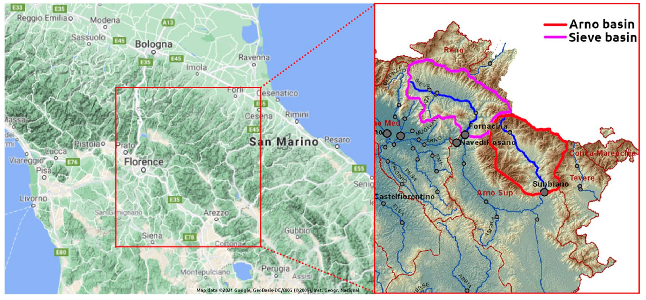
KNN and Bluecat were applied in two case studies, Arno River at Subbiano and Sieve River at Fornacina. Sieve River is a tributary of Arno River. They both flow in the Tuscany Region, Italy. Figure 1 presents a schematic map of Arno River and Sieve River basins.
The catchment of Arno River is 752 km2. The observed data include the mean areal daily rainfall, the evapotranspiration, and the discharge at the basin exit. The period of the available data starts from 2 January 1992 and ends on 1 January 2014.
The catchment area of Sieve River is 846 km2. The observed data include the mean areal hourly rainfall, the evapotranspiration, and the discharge at the basin exit. The period of the available data starts from 3 June 1992 and ends on 2 January 1997 (there is a gap in the data from 1 January 1995 to 2 June 1995). The flow regime of Sieve River is intermittent, 4% of the observed streamflow values are zero.
The streamflows of the two catchments were simulated with the hydrological model HyMod [16,17]. It should be stressed that the structure and characteristics of this hydrological model did not play any role in the estimation of the uncertainty, which is carried out exclusively based on the available data. The data of Arno River and Sieve River case studies were split (without shuffling) into training and test tests. These two sets correspond to the calibration and validation of HyMod. The split ratio was 91:9 for Arno River (8036 total data records) and 62:38 for Sieve River (36,554 total data records).
2.2. Estimate Uncertainty with KNN
An intuitive approach to estimate the uncertainty of a simulation value of a hydrological model would be to analyse the model behaviour during a period with available measurements and when the model was in states similar to that producing the assessed simulation value. This would include the following steps, first identify a number of occasions when the model was in a similar state, then, fetch the corresponding observations. If the hydrological model represents consistently the hydrological process, the fetched observations, which correspond to similar states of the model, will be similar. On the contrary, an increased variance of the fetched observations would imply an increased uncertainty whenever the model is in a state similar to the one assessed. Therefore, the statistical analysis of the fetched observations can provide information regarding the uncertainty of the assessed simulation value.
The previously mentioned idea resembles the concept behind the k-nearest neighbours (KNN) method. “KNN algorithm assumes the similarity between the new case/data and available cases and puts the new case into the category that is most similar to the available categories. KNN algorithm can be used for regression as well as for classification” [18]. KNN is an instance-based non-parametric model [19]. It is non-parametric because it depends on the available data to operate (in contrast, parametric models need the data only during the model training), and instance-based because it is based on resemblance with instances in the training set to make inference (instead of employing explicit operations).
KNN has been already applied by other researchers for estimating the uncertainty of hydrological models as part of complicated frameworks. For example, Sikorska et al. [9], have included KNN in Monte Carlo simulations for estimating the prediction limits. In this study, we employ a simpler data-driven approach, similar to the one employed in Bluecat [12]. KNN returns a set of observations made during an earlier period of that of the assessed simulation value that are related (i.e., correspond to a similar model state) to the assessed simulation value. Then, the uncertainty can be estimated with the following formula:
where s is a value related to the uncertainty of the value simulated by the hydrological model when it is in the state x, x is a vector (or a scalar) that defines the state of the model (the features in machine learning terminology), KNN(k, x) returns the set of the k observations that according to KNN are those most related to x, and f: ℝk → ℝ is a function that returns a value related with some statistical property of the set returned by KNN(k, x), in the typical regression applications of KNN this is the average. The previous quantities refer to the time instance t of a simulation obtained by the hydrological model. The symbol of the variable t is omitted from Equation (1) for the sake of simplicity (normally should appear either as a subscript or superscript).
s = f(KNN(k, x))
In this study, three functions were employed as f in Equation (1). The 90th percentile, the 10th percentile (these are the bounds of the 80% confidence interval), and the median value. Regarding the parameter k, this is a hyperparameter. A low k value will result in overfitting whereas a high k value in underfitting [19] and bias (see the Discussion section). The values of this parameter can range from 10 (for a small observation dataset) up to 1000 (for a large, say hundreds of thousands of records, dataset). Regarding the vector x, the following options were tested:
- 1D. One dimensional, this is the simplest approach that includes only the assessed discharge simulated by the hydrological model at the time step t, x = Qt. KNN returns the k observations that correspond to the k simulated discharges of the calibration period that are the closest to Qt.
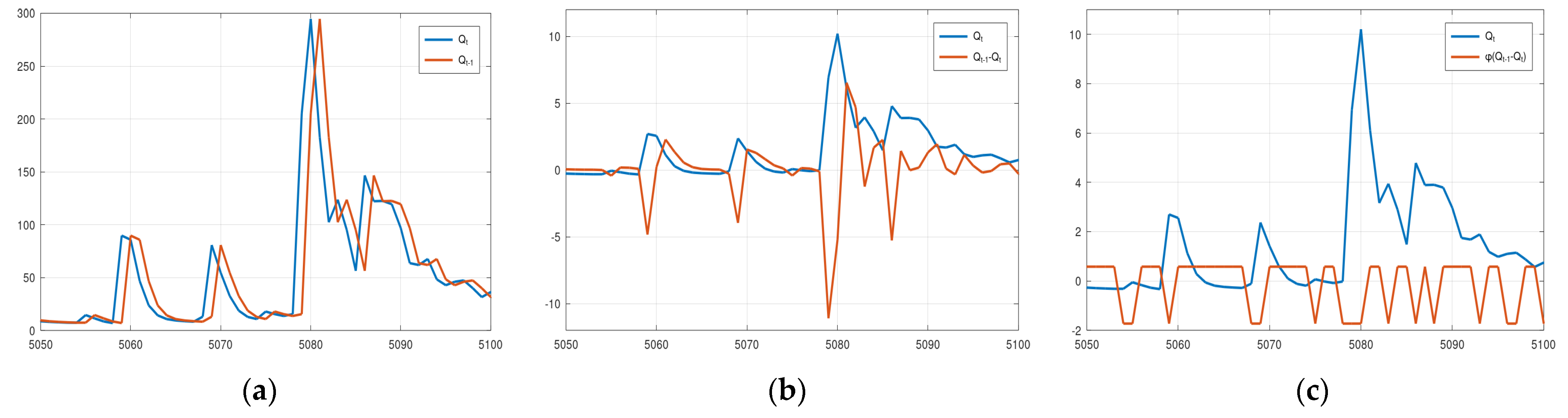
- 2D Option 1. The vector elements are two successive simulated discharges, x = (Qt, Qt−1), KNN returns the k observations that correspond to the k vectors of the calibration period that are closer in the 2D Euclidean space to the vector (Qt, Qt−1).
- 2D Option 2. The vector elements are the discharge Qt and the change of the simulated discharge between t − 1 and t, x= (Qt, Qt−1 − Qt).
- 2D Option 3. The vector elements are the discharge Qt and a binary value, 0 if the discharge increases and 1 if it does not increase, this binary value can be obtained with the function φ(⋅) = max(0, (⋅)/|⋅|), x = (Qt, φ(Qt−1 − Qt)).
In the last two options, the elements of vector x (i.e., the features) need to be scaled so that the Euclidean distance is equally sensitive to both dimensions. For this reason, the z-score normalisation was employed [20]. To avoid data leakage [21], the normalisation parameters (i.e., the mean and standard deviation) were obtained from the training set only, and then the normalisation was applied to both sets.
The time complexity for KNN to identify the nearest neighbours in a set of n records is O(n) when the naive method is used, O(log n) when the binary tree method is used, and O(1) when a hash table is used [19](pp. 739). In this study, the tool mlpack_knn from the package mlpack was run with the option of using dual tree for obtaining the nearest neighbours [22].
2.3. Estimate Uncertainty with Bluecat
In Bluecat, the uncertainty of a simulation value is estimated with the conditional distribution Fq|Q(q|Q), which is defined by the following formula.
where q and Q are specific values of the observed discharge and the discharge simulated by the hydrological model, respectively, q is the stochastic process that corresponds to the studied discharge, and Q is the stochastic process that corresponds to the simulated discharge.
Fq|Q(q|Q) ≔ P{q ≤ q|Q = Q }
The typical approach to estimate the probability at the right hand of Equation (2) is to use Bayesian inference.
where N(⋅) is a function that returns the frequency of occurrences of the event given within the parentheses, i.e., N(Q = Q|q ≤ q) is the inverse of the number of times the observed discharge is less than q during the calibration period multiplied by the number of times the simulated discharge is Q when on the same time the observed discharge is less than q, N(q ≤ q) is 1/n (n is the length of observations) multiplied by the number of times the observed discharge is less than q, and N(Q = Q) is 1/n multiplied by number of times the simulated discharge is Q.
P{q ≤ q|Q = Q} = N(Q = Q|q ≤ q) × N(q ≤ q)/N(Q = Q)
As the variables of interest in hydrology are of continuous type, we may expect that each value Q of the simulated time series is very uncommon to appear multiple times. As a result, N(Q = Q) will always be 1/n, and N(Q = Q|q ≤ q) will be non-continuous taking only the values 0 and the inverse of the number of times the observed discharge is less than q. For this reason, Koutsoyiannis and Montanari suggested an approximative estimation of the conditional distribution using the following formula.
where ΔQ1 and ΔQ2 define a neighbourhood of Q such that the intervals above and below Q contain appropriate numbers of simulation values, say 2m + 1 if the closest plus an equal number of m values above and below Q is selected.
Fq|Q(q|Q) ≈ P{q ≤ q|Q − ΔQ1 ≤ Q ≤ Q + ΔQ2}
Using Equation (4), the median and the 80% confidence interval can be obtained, which will be compared with the results obtained with KNN.
3. Results
This section provides the results of KNN and Bluecat applied in the two case studies (Arno River at Subbiano and Sieve River at Fornacina). The results are displayed employing (i) plots of the simulation values during the validation period, including the upper and lower bounds of the 80% confidence interval, and the median value; (ii) the scatter plots of the confidence interval, the median, and the observed values against the values simulated by the hydrological model (HyMod in these case studies); and (iii) the combined probability-probability plots of the median and the hydrological model values.
Regarding the plots of the simulation values, the criteria of the quantitative evaluation are the proximity of the median values to the corresponding observed values, and the successful envelopment of most of the observations by the confidence interval (approximately 10% should be above the upper limit and 10% below the lower limit).
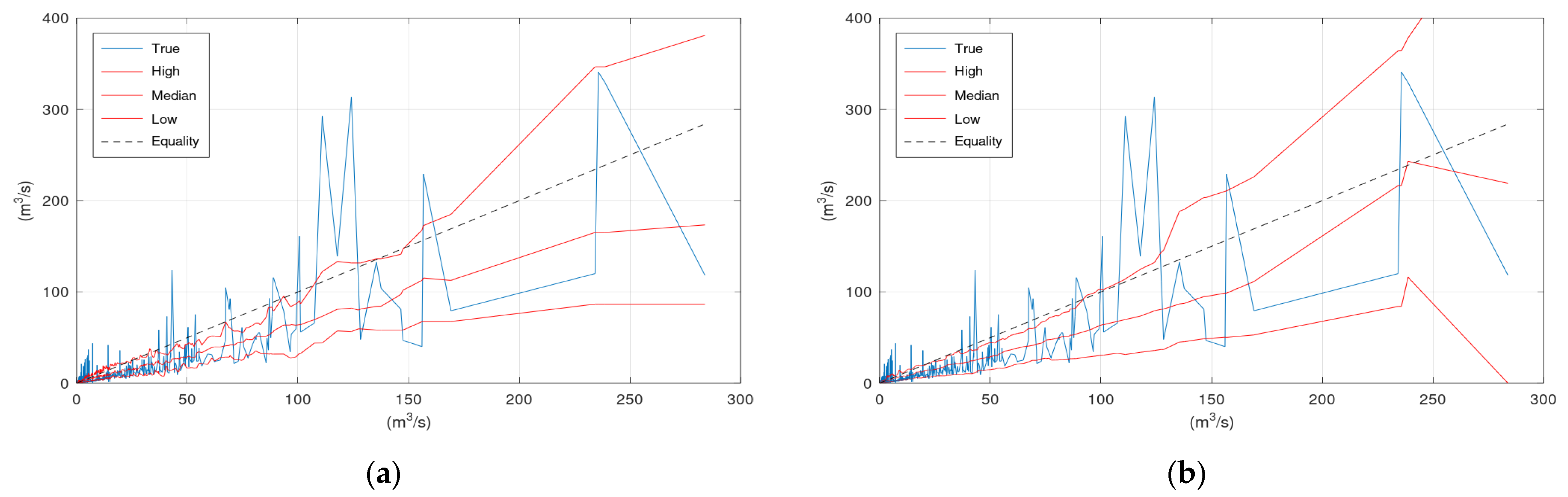
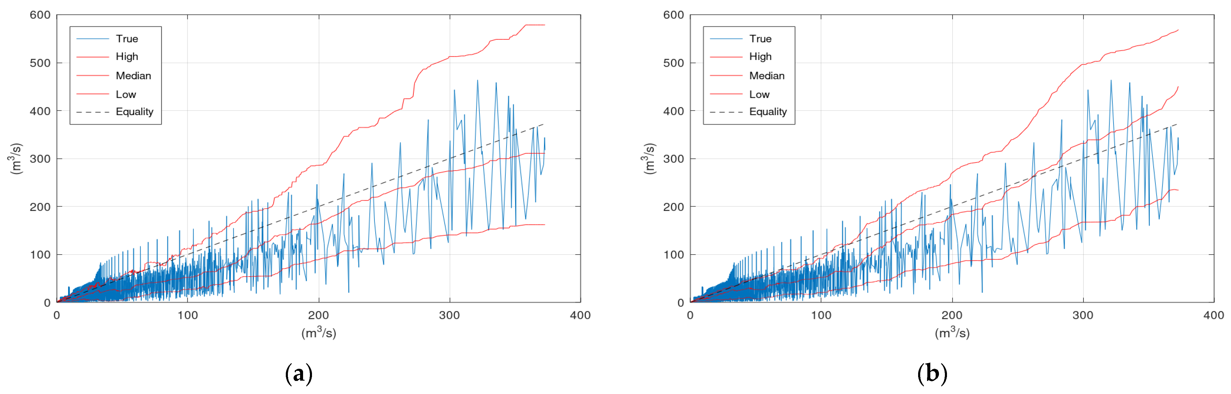
The scatter plots include in the x-axis the sorted simulation values of the hydraulic model. The line labelled “True” is obtained when the y-axis refers to the corresponding observed values, the line labelled “Median” when the y-axis refers to the corresponding median values, the line labelled “High” when the y-axis refers to the corresponding upper bound of the 80% confidence interval, and the line labelled “Low” when the y-axis refers to the corresponding lower bound of the 80% confidence interval. A deviation of the Equality line from the “True” line indicates errors or bias in the hydrological model. The smoother the “True” line, the lower the model errors. The spikes of the “True” line should be evenly placed above and below the Equality line, otherwise the model introduces bias. Regarding the KNN and Bluecat outputs, the “Median” should lay close to the “True” line (for the same reason the Equality line should be close to the “True” line). The percentage of the “True” line outside the “High” and “Low” lines should be equal to the selected confidence level. Ideally, this percentage should not be influenced by the magnitude of the simulation value.
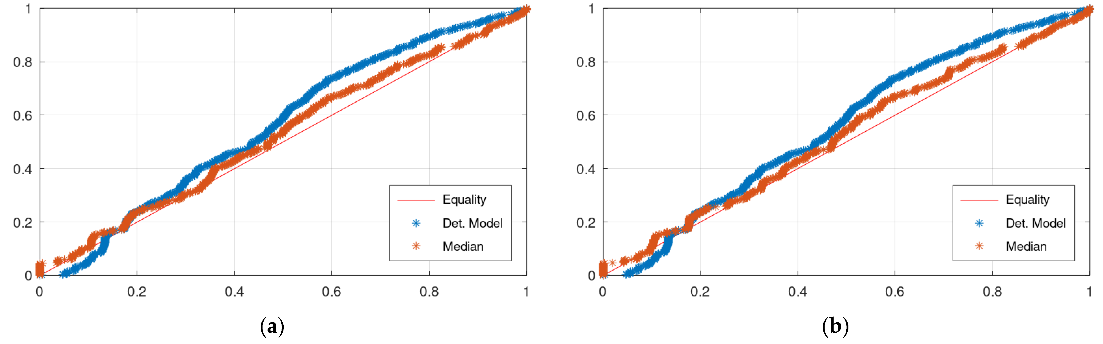
The combined probability-probability (CPP) plot is the plot of the values of the empirical distribution function of the median from KNN or Bluecat, or the hydrological model simulations (y-axis) against the corresponding values of the empirical distribution function of the observations (x-axis). Ideally, the CPP plot should be on the Equality line.
The scatter plots are superior in assessing the performance of a model at extreme values, where there are usually very few simulated and observed values. At this range, even if there is a significant deviation between these two, the difference between the corresponding values of the empirical distributions could be negligible because of the limited number of values at this range compared to the number of values in the whole assessed period. Thus, this small difference (e.g., 0.97 against 0.99) will pass unnoticed in the CPP plot. On the other hand, CPP plots are better for assessing the performance of a model at the range where the majority of simulations/observations occur.
3.1. Case Study—Arno
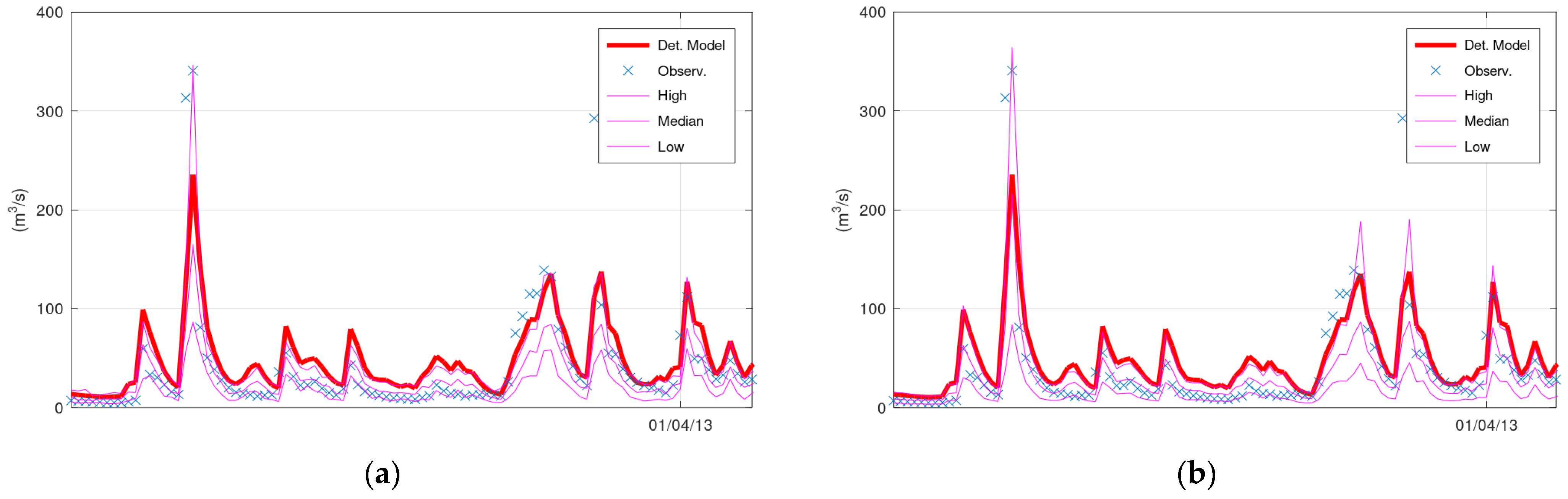
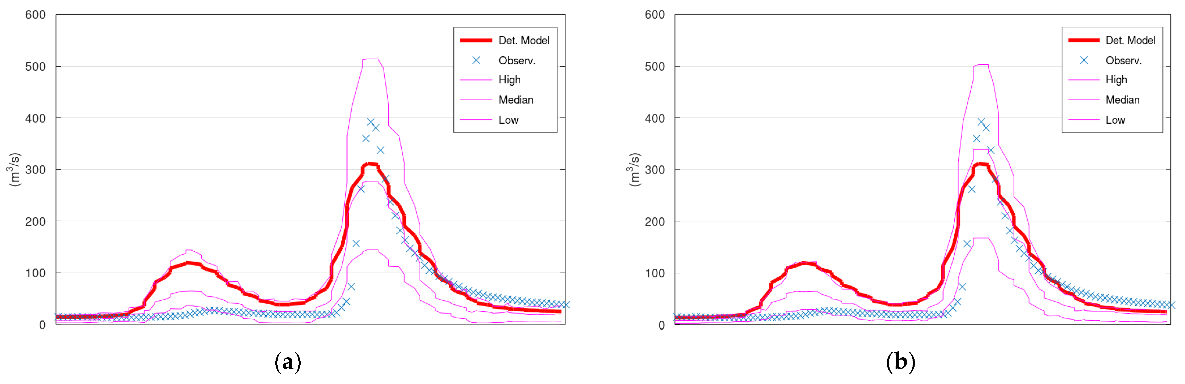
Figure 2 displays the simulated discharge of 100 days (out of the 731 in total) of the validation period (from 1 January 2013 until 11 April 2013), the corresponding confidence interval (“High” and “Low” lines), and the median values of KNN and Bluecat. The left panel displays the results of KNN with 40 neighbours, whereas the right panel displays the results of Bluecat. There are minor differences between these two figures regarding the confidence interval bounds at the two peaks before 1 April 2013.
Figure 3 displays the scatter plots of the application of KNN and Bluecat to the validation period of the Arno River case study. Significant differences between the plots of the two models appear in the region of very high flows. These differences are related to the limited number of observations and simulations at this range of values.
Figure 4 displays the CPP of the application of KNN and Bluecat to the validation period of the Arno River case study. The differences between the plots of the two models are insignificant.
3.2. Case Study—Sieve
Figure 5 displays the simulated discharge of 150 h (out of the 13,896 in total) of the validation period (starting from 5 January 1996), the corresponding confidence interval (“High” and “Low” lines) and the median values of KNN and Bluecat. The left panel displays the results of KNN with 200 neighbours, whereas the right panel displays the results of Bluecat. The median values of Bluecat appear closer to the observed values around the peak of this figure.
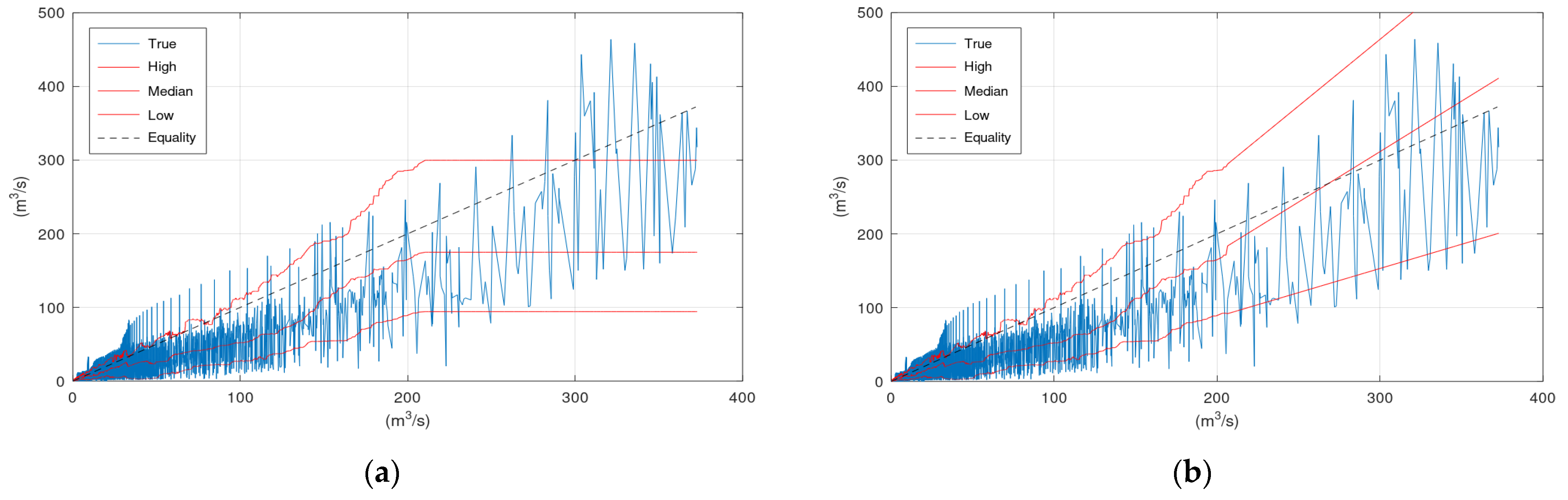
Figure 6 displays the scatter plots of the application of KNN and Bluecat to the validation period of the Sieve River case study. The “High” lines of KNN and Bluecat are very similar with minor differences at discharges around 200 m3/s. The “Low” line of Bluecat tends to be higher at high flows. The “Median” line of Bluecat seems to deviate from the “True” line at high flows.
Figure 7 displays the CPP of the application of KNN and Bluecat to the validation period of the Sieve River case study. The CPP of KNN appears slightly closer to the Equality line.
4. Discussion
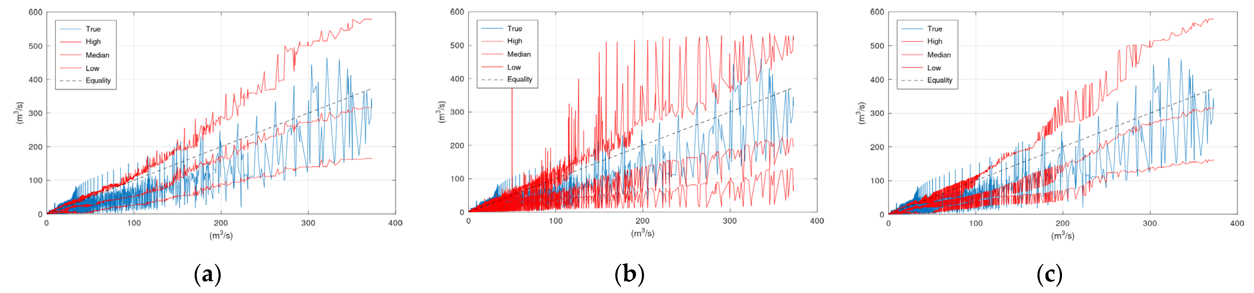
Regarding the three 2D options for sampling the model status, the basic idea for increasing the dimension of the sampling space was that this could discriminate between the rising and falling limbs of the hydrograph. A hydrological model may exhibit different magnitudes of errors when switching from one condition (rising) to another (recession), which could be captured by the 2D sampling. Option 1 includes the assessed discharge and the discharge of the previous step, Option 2 includes the assessed discharge and the change, and Option 3 includes the discharge and a binary value, 0 for rising and 1 for recession. An assessment of the properties of the Euclidean metric reveals that Option 1 may not be always appropriate for distinguishing between the rising and falling limbs. For example, suppose the assessed hydrological model with status vector (Qt, Qt−1), where Qt = 99 and Qt−1 = 100. In this case, the vector (100, 99) is closer to the assessed status vector than the vector (100, 102). Yet the former corresponds to a rising part of the hydrograph, whereas the latter and the status vector correspond to a recession. The distinction between rising and falling limbs of the hydrograph is guaranteed with Option 2 and Option 3. However, these options may overemphasise this distinction. For example, Figure 8 displays the plots of the elements (a.k.a. features) of status vector x for the three 2D options (normalised values in Options 2 and 3) for the Arno River case study. It is evident that in Option 2 two status vectors corresponding to successive simulated discharges may have very large Euclidean distance because the difference Qt−1 − Qt fluctuates strongly when passing from the rising to the falling limb (Figure 8b before and after 5080). This is probably the reason the boundaries of the confidence interval and the median value in Figure A2b exhibit the intense fluctuations. This effect is mitigated in Option 3. However, according to Figure A1 and Figure A2 neither option appears to offer any advantage over the simplest 1D option. It should be noted that this may be happening just because the error of the hydrological model used in this study and for these specific two case studies is similar in the rising and falling parts of the hydrograph. If this is the case, then the uncertainty depends only on the model output and not on its state. Therefore, the model output alone can be used in a data-driven method to obtain estimations of its uncertainty.
The results of KNN and Blueacat displayed in Figure 2, Figure 3, Figure 4, Figure 5, Figure 6 and Figure 7 indicate only insignificant differences between the two methods. Figure 3 and Figure 6 indicate that the “Median” line is closer to the “True” line than the Equality line, which means that the former is less biassed compared to the simulation values (Table 1). Furthermore, the upper bound of the 80% confidence interval has encapsulated the more extreme events in both case studies indicating that this would be a more reliable signal than the hydrological model simulation to be used in an early warning system. Finally, Figure 4 and Figure 7 indicate that the CPP line of the median values is closer to the Equality line, which means that the median value would be useful in applications of water resources management.
Regarding the insignificant differences between the two methods, a closer inspection of the theory behind them reveals algorithmic similarities. Applying Bayesian inference to Equation (4) gives,
where mQ, is the number of simulation values within the range (Q − ΔQ1, Q + ΔQ2) of which the corresponding observations are less than q, nq is the number of observations that are less than q, n is the total number of observations, and 2m + 1 is the predetermined total number of simulation values within the range (Q − ΔQ1, Q + ΔQ2).
Fq|Q(q|Q) ≈ (mQ/nq) × (nq/n)/((2m + 1)/n) = mQ/(2m + 1)
To obtain the number mQ, the observations that correspond to the 2m + 1 simulations within the range (Q − ΔQ1, Q + ΔQ2) need to be identified. These observations are more or less the output of KNN(k, x) in Equation (1) with only one difference, Equation (1) does not take extra care to ensure an equal number of values above and below Q. Furthermore, the right side of Equation (5) is the empirical distribution of the 2m + 1 observations. It is exactly the inverse of this empirical distribution that is used as f in Equation (1) to obtain the 90th and 10th percentiles, and the median value.
The previously mentioned difference between KNN and Bluecat regarding the selection of neighbours may result in a biased estimation of the conditional distribution Fq|Q(q|Q) at high and low Q by KNN because of an unbalanced number of values below and above Q. That is, the higher the assessed value Q the less the number of simulated values in the calibration period higher than Q. As a result, for very high Q values, KNN will return mostly observations corresponding to neighbours of Q lower than Q. This bias is the reason that the upper bound of the 80% confidence interval in Figure 2a coincides with the hydrological model simulation at the two peaks before 1 April 2013. It is also the reason for the differences between Figure 3a,b.
In both case studies, the maximum simulated discharge during the validation period was significantly lower than the maximum simulated discharge during the calibration. This allowed a sufficient number of neighbours above any Q value, even for the maximum Q value of the validation. However, it is not guaranteed this will be the case in every hydrological application. Recently, Koutsoyiannis and Montanari suggested a technique to address this issue [23]. In this study, we suggest a simpler approach, which is inspired by the scatter plots in Figure 3 and Figure 6.
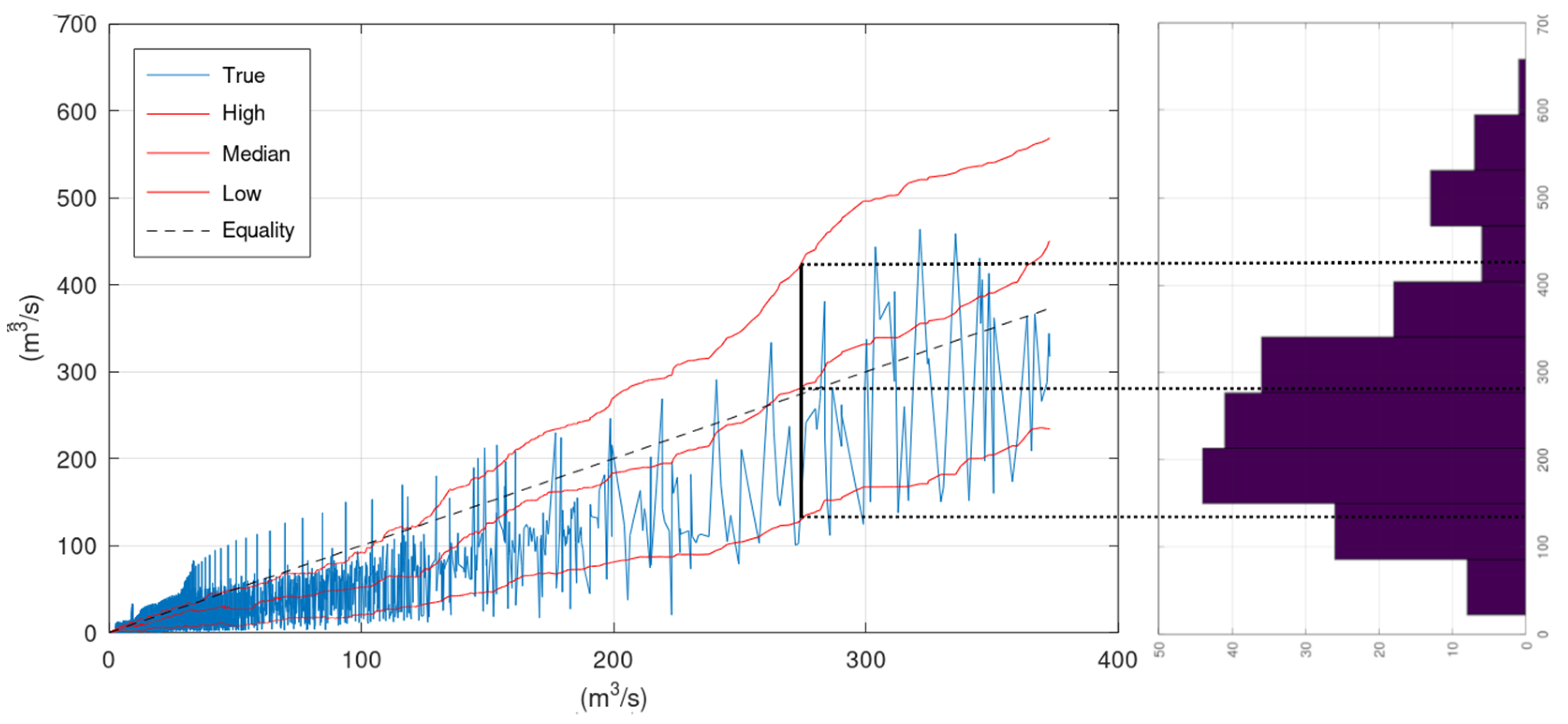
On the right side of Figure 9 lies the histogram of the observations that correspond to the simulated by the hydrological model values that are closer to the assessed simulation value of 275 m3/s. A rough representation of this histogram can be obtained by the values of the upper and lower confidence interval bounds and the median value that correspond to 275 m3/s (see vertical black and dotted lines in Figure 9). Therefore, the lines “High”, “Median”, and “Low” provide a rough representation of the histograms (or the graphical representation of the probability density function of Fq|Q(q|Q)) of all assessed Q values.
KNN and Bluecat can draw these three lines up to the Q value of the validation period that is covered by a sufficient number of greater discharges simulated by the hydrological model during the calibration period. The simplest approach to extend these three lines beyond this specific Q value, and, consequently, to obtain an estimation of the conditional distribution Fq|Q(q|Q) for Q values beyond the available information, is to extrapolate them with linear regression. The application of this simple approach for the two case studies is demonstrated in Appendix B.
5. Conclusions
In this study, we have employed a statistical data-driven method (Bluecat) and a machine learning method (k-nearest neighbours) to assess the uncertainty of a hydrological model simulation. The two methods were applied in two real-world case studies. The lessons from these applications were the following.
- The machine learning method is more flexible than the statistical method, which allows using more complex sampling schemes at higher dimensions (e.g., model simulation values from multiple time steps). This may improve the reliability of the estimated uncertainty in some cases. However, the application in the two case studies did not prove any advantage over the simplest approach (1D sampling, only the discharge). This finding cannot be generalized since it depends on the performance of the selected hydrological model in each specific case study. Nevertheless, it appears that the simplest approach captures successfully most (if not all) of the characteristics of the uncertainty.
- Machine learning is usually considered a black-box approach with some abstract/intuitive understanding of its functionality. However, in some applications, a close inspection can reveal similarities, or even equivalency, with rigorous mathematical approaches. The identification of the deviations of the algorithm underneath a machine learning method from the rigorous approach allows detecting the conditions under which the machine learning model may exhibit poor performance, and thus, increase its credibility.
- A very simple approach based on linear regression was employed to estimate the statistical structure of the assessed hydrological model uncertainty at conditions never met in the available data. This approach was tested in the two case studies and was found to perform satisfactorily.
The data-driven analysis of the uncertainty of the hydrological model (based on machine learning or statistical theory) in the two case studies can offer not only an estimation of the confidence we can have in the model results, but also operational benefits. For example, the median values had significantly less bias than the values simulated by the hydrological model. More specifically, the hydrological model overestimated the mean discharge by 50% whereas the median values by only 4%. Therefore, the median values can be more useful in applications of water resources management. Similarly, appropriate confidence levels, corresponding to an acceptable risk, could be selected to obtain probabilistic estimations of extreme values providing more reliable early warning systems. The latter requires research on the main weakness of the data-driven methods, i.e., the estimation of the uncertainty at conditions never met in the available data. A more thorough assessment of the simple approach (linear regression) employed here should be performed and more elaborated approaches (e.g., multi-layer perceptrons) need to be considered, which may prove more advantageous.
Author Contributions
Conceptualization, E.R., D.K. and A.M.; methodology, E.R.; software, E.R. and A.M.; validation, E.R. and D.K.; formal analysis, E.R.; investigation, E.R.; resources, E.R.; data curation, A.M.; writing—original draft preparation, E.R.; writing—review and editing, D.K. and A.M.; visualization, E.R.; supervision, E.R.; project administration, E.R.; funding acquisition, not applicable. All authors have read and agreed to the published version of the manuscript.
Funding
This research received no external funding.
Institutional Review Board Statement
Not applicable.
Informed Consent Statement
Not applicable.
Data Availability Statement
The hydrological model of this study is available for download at the web address: https://github.com/albertomontanari/hymodbluecat (accessed on 8 April 2022) along with instructions to compile it in R. The data of the two case studies are also included at this link. A tool suitable for practitioners will be made publicly available upon publication at http://hydronoa.gr (accessed on 1 February 2022).
Conflicts of Interest
The authors declare no conflict of interest.
Appendix A
The following figures display the scatter plots of the application of KNN to the validation period of Arno River for the three types of 2D sampling.
Figure A1.
Scatter plot of the KNN application in the Arno River case study during the validation period: (a) 2D Option 1; (b) 2D Option 2; (c) 2D Option 3.
Figure A1.
Scatter plot of the KNN application in the Arno River case study during the validation period: (a) 2D Option 1; (b) 2D Option 2; (c) 2D Option 3.

The following figures display the scatter plots of the application of KNN to the validation period of Sieve River for the three types of 2D sampling.
Figure A2.
Scatter plot of the KNN application in the Sieve River case study during the validation period: (a) 2D Option 1; (b) 2D Option 2; (c) 2D Option 3.
Figure A2.
Scatter plot of the KNN application in the Sieve River case study during the validation period: (a) 2D Option 1; (b) 2D Option 2; (c) 2D Option 3.

Appendix B
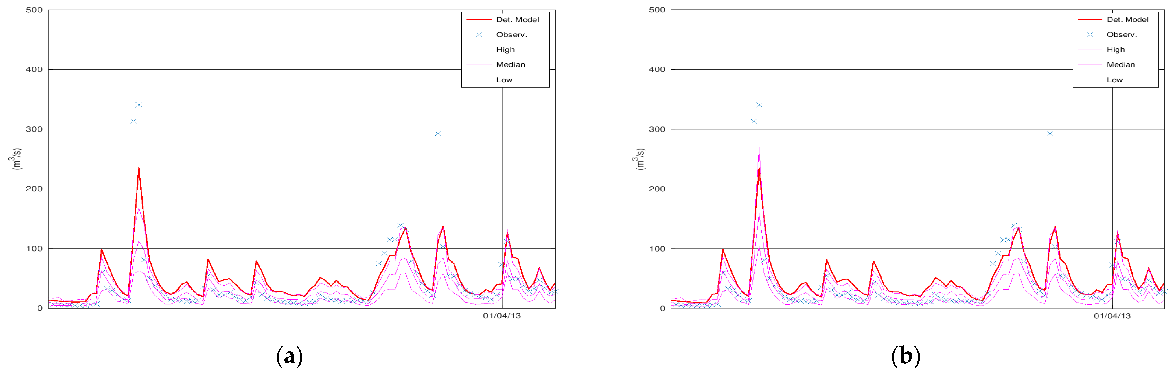
To evaluate the suggested extrapolation method, the simulated discharge values from the hydrological model greater than a specific value were removed from the calibration set, which resulted in a trimmed training data set (the set that is used by KNN to fetch the observations corresponding to the nearest simulated values). This specific value was 200 and 350 m3/s for the Arno River and Sieve River case studies, respectively. The results when applying the extrapolation method are displayed in the following figures.
Figure A3.
Discharge of Arno River, 100 daily time steps of the validation period starting from 1 January 2013: (a) KNN applied to the trimmed training data set; (b) KNN with linear extrapolation applied to the trimmed training data set. “Det. Model” is the simulation with HyMod.
Figure A3.
Discharge of Arno River, 100 daily time steps of the validation period starting from 1 January 2013: (a) KNN applied to the trimmed training data set; (b) KNN with linear extrapolation applied to the trimmed training data set. “Det. Model” is the simulation with HyMod.

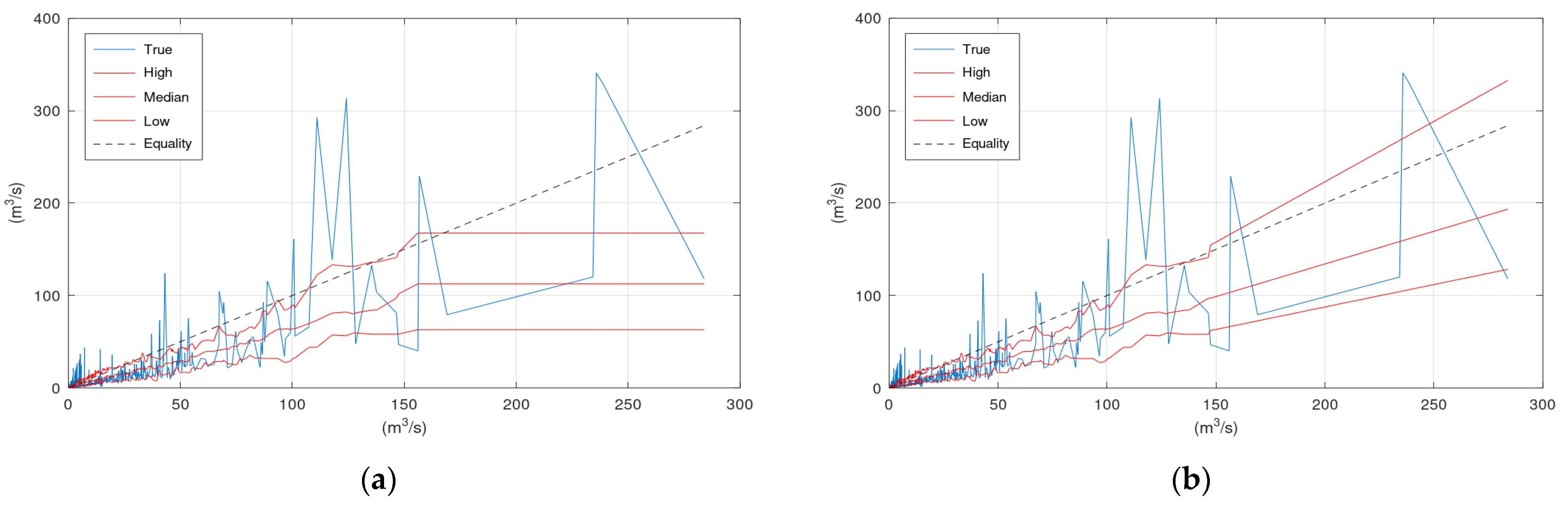
Figure A4.
Scatter plot of Arno River case study: (a) KNN applied to the trimmed training data set; (b) KNN with linear extrapolation applied to the trimmed training data set.
Figure A4.
Scatter plot of Arno River case study: (a) KNN applied to the trimmed training data set; (b) KNN with linear extrapolation applied to the trimmed training data set.

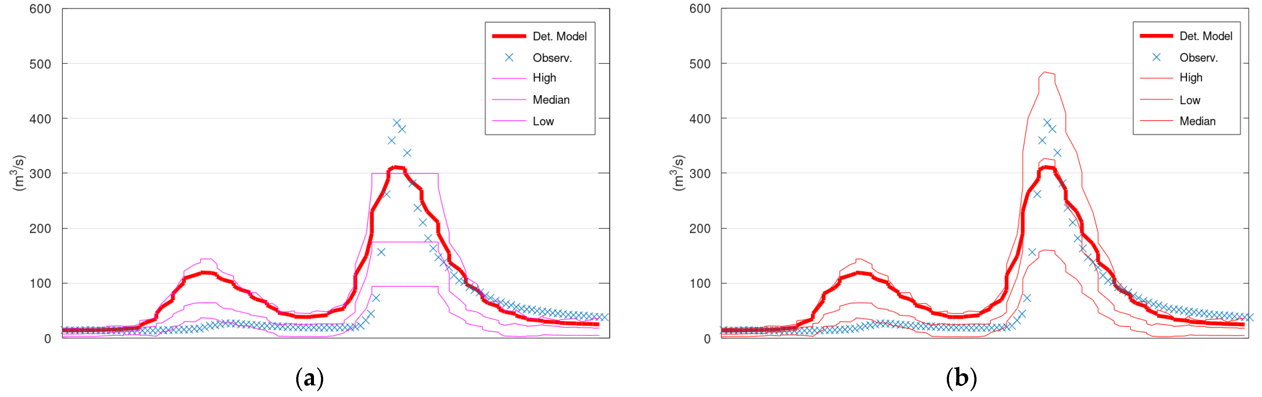
Figure A5.
Discharge of Sieve River, 150 hourly time steps of the validation period starting from 5 January 1996: (a) KNN applied to the trimmed training data set; (b) KNN with linear extrapolation applied to the trimmed training data set. “Det. Model” is the simulation with HyMod.
Figure A5.
Discharge of Sieve River, 150 hourly time steps of the validation period starting from 5 January 1996: (a) KNN applied to the trimmed training data set; (b) KNN with linear extrapolation applied to the trimmed training data set. “Det. Model” is the simulation with HyMod.

Figure A6.
Scatter plot of the Sieve River case study: (a) KNN applied to the trimmed training data set; (b) KNN with linear extrapolation applied to the trimmed training data set.
Figure A6.
Scatter plot of the Sieve River case study: (a) KNN applied to the trimmed training data set; (b) KNN with linear extrapolation applied to the trimmed training data set.

References
- Rosenblatt, F. The Perceptron, a Perceiving and Recognizing Automaton Project Para; Cornell Aeronautical Laboratory, Inc.: Buffalo, NY, USA, 1957. [Google Scholar]
- Minsky, M.; Papert, S. Perceptrons: An Introduction to Computational Geometry; MIT Press: Cambridge, MA, USA, 1969. [Google Scholar]
- Rumelhart, D.; Hinton, G.; Williams, R. Learning representations by back-propagating errors. Nature 1986, 323, 533–536. [Google Scholar] [CrossRef]
- Shen, C.; Laloy, E.; Elshorbagy, A.; Albert, A.; Bales, J.; Chang, F.; Ganguly, S.; Hsu, K.; Kifer, D.; Fang, Z.; et al. HESS Opinions: Incubating deep-learning-powered hydrologic science advances as a community. Hydrol. Earth Syst. Sci. 2018, 22, 5639–5656. [Google Scholar] [CrossRef] [Green Version]
- Shen, C. A Transdisciplinary Review of Deep Learning Research and Its Relevance for Water Resources Scientists. Water Resour. Res. 2018, 54, 8558–8593. [Google Scholar] [CrossRef]
- Rozos, E.; Dimitriadis, P.; Mazi, K.; Koussis, A.D. A Multilayer Perceptron Model for Stochastic Synthesis. Hydrology 2021, 8, 67. [Google Scholar] [CrossRef]
- Rozos, E.; Dimitriadis, P.; Bellos, V. Machine Learning in Assessing the Performance of Hydrological Models. Hydrology 2022, 9, 5. [Google Scholar] [CrossRef]
- Sikorska-Senoner, A.; Quilty, J. A novel ensemble-based conceptual-data-driven approach for improved streamflow simulations. Environ. Model. Softw. 2021, 143, 105094. [Google Scholar] [CrossRef]
- Sikorska, A.; Montanari, A.; Koutsoyiannis, D. Estimating the Uncertainty of Hydrological Predictions through Data-Driven Resampling Techniques. J. Hydrol. Eng. 2015, 20, A4014009. [Google Scholar] [CrossRef]
- Solomatine, D.P.; Shrestha, D.L. A novel method to estimate model uncertainty using machine learning techniques. Water Resour. Res. 2009, 45, W00B11. [Google Scholar] [CrossRef]
- Karlsson, M.; Yakowitz, S. Nearest-neighbor methods for nonparametric rainfall-runoff forecasting. Water Resour. Res. 1987, 23, 1300–1308. [Google Scholar] [CrossRef]
- Koutsoyiannis, D.; Montanari, A. Bluecat: A Local Uncertainty Estimator for Deterministic Simulations and Predictions. Water Resour. Res. 2022, 58, e2021WR031215. [Google Scholar] [CrossRef]
- Ehteram, M.; Mousavi, S.; Karami, H.; Farzin, S.; Singh, V.; Chau, K.; El-Shafie, A. Reservoir operation based on evolutionary algorithms and multi-criteria decision-making under climate change and uncertainty. J. Hydroinformatics 2018, 20, 332–355. [Google Scholar] [CrossRef]
- Sharafati, A.; Pezeshki, E. A strategy to assess the uncertainty of a climate change impact on extreme hydrological events in the semi-arid Dehbar catchment in Iran. Theor. Appl. Climatol. 2019, 139, 389–402. [Google Scholar] [CrossRef]
- Zhao, C.; Huang, Y.; Li, Z.; Chen, M. Drought Monitoring of Southwestern China Using Insufficient GRACE Data for the Long-Term Mean Reference Frame under Global Change. J. Clim. 2018, 31, 6897–6911. [Google Scholar] [CrossRef]
- Boyle, D. Multicriteria Calibration of Hydrological Models. Doctoral Dissertation, University of Arizona, Tucson, AZ, USA, 2000, unpublished. [Google Scholar]
- Montanari, A. Large sample behaviors of the generalized likelihood uncertainty estimation (GLUE) in assessing the uncertainty of rainfall-runoff simulations. Water Resour. Res. 2005, 41. [Google Scholar] [CrossRef]
- K-Nearest Neighbor(KNN) Algorithm for Machine Learning—Javatpoint. Available online: https://www.javatpoint.com/k-nearest-neighbor-algorithm-for-machine-learning (accessed on 12 May 2022).
- Russell, S.; Norvig, P. Artificial Intelligence; Prentice-Hall: Upper Saddle River, NJ, USA, 2010. [Google Scholar]
- Jordan, J. Normalizing Your Data (Specifically, Input and Batch Normalization). 2021. Available online: https://www.jeremyjordan.me/batch-normalization/ (accessed on 2 February 2021).
- Preventing Data Leakage in Your Machine Learning Model. Available online: https://towardsdatascience.com/preventing-data-leakage-in-your-machine-learning-model-9ae54b3cd1fb (accessed on 1 May 2022).
- Documentation mlpack-3-4-2. Available online: https://www.mlpack.org/doc/stable/cli_documentation.html#knn (accessed on 4 May 2022).
- Koutsoyiannis, D.; Montanari, A. Climate Extrapolations in Hydrology: The Expanded Bluecat Methodology. Hydrology 2022, 9, 86. [Google Scholar] [CrossRef]
Figure 1.
Basins of Arno River at Subbiano and Sieve River at Fornacina.

Figure 2.
Discharge of Arno River, 100 days of the validation period starting from 1 January 2013: (a) KNN; (b) Bluecat. “Det. Model” is the simulation with HyMod.
Figure 2.
Discharge of Arno River, 100 days of the validation period starting from 1 January 2013: (a) KNN; (b) Bluecat. “Det. Model” is the simulation with HyMod.

Figure 3.
Scatter plot of the Arno River case study: (a) KNN; (b) Bluecat.

Figure 4.
CPP plots of the Arno River case study: (a) KNN; (b) Bluecat. “Det. Model” is the simulation with HyMod.
Figure 4.
CPP plots of the Arno River case study: (a) KNN; (b) Bluecat. “Det. Model” is the simulation with HyMod.

Figure 5.
Discharge of Sieve River, 150 hourly time steps of the validation period starting from 5 January 1996: (a) KNN; (b) Bluecat. “Det. Model” is the simulation with HyMod.
Figure 5.
Discharge of Sieve River, 150 hourly time steps of the validation period starting from 5 January 1996: (a) KNN; (b) Bluecat. “Det. Model” is the simulation with HyMod.

Figure 6.
Scatter plot of the Sieve River case study: (a) KNN; (b) Bluecat.

Figure 7.
CPP plots of the Sieve River case study: (a) KNN; (b) Bluecat. “Det. Model” is the simulation with HyMod.
Figure 7.
CPP plots of the Sieve River case study: (a) KNN; (b) Bluecat. “Det. Model” is the simulation with HyMod.

Figure 8.
The elements of status vector x: (a) 2D Option 1; (b) 2D Option 2; (c) 2D Option 3.

Figure 9.
Visual explanation of confidence interval bound and median line for the discharge value of the hydrological simulation during the validation period equal to 275 m3/s (case study of Sieve River). The histogram on the right organises in classes the observed values that correspond to the 200 simulation values closer to 275 m3/s.


Table 1.
Mean value of the time series of observations, of the HyMod simulation, and of the Bluecat Median and KNN Median.
Table 1.
Mean value of the time series of observations, of the HyMod simulation, and of the Bluecat Median and KNN Median.
| Observations (m3/s) | HyMod (m3/s) | Bluecat Median (m3/s) | KNN Median (m3/s) | |
|---|---|---|---|---|
| Arno River | 10.98 | 16.24 | 12.24 | 11.32 |
| Sieve River | 12.56 | 17.79 | 11.78 | 11.58 |
Publisher’s Note: MDPI stays neutral with regard to jurisdictional claims in published maps and institutional affiliations. |
© 2022 by the authors. Licensee MDPI, Basel, Switzerland. This article is an open access article distributed under the terms and conditions of the Creative Commons Attribution (CC BY) license (https://creativecommons.org/licenses/by/4.0/).
Share and Cite
MDPI and ACS Style
Rozos, E.; Koutsoyiannis, D.; Montanari, A. KNN vs. Bluecat—Machine Learning vs. Classical Statistics. Hydrology 2022, 9, 101. https://0-doi-org.brum.beds.ac.uk/10.3390/hydrology9060101
AMA Style
Rozos E, Koutsoyiannis D, Montanari A. KNN vs. Bluecat—Machine Learning vs. Classical Statistics. Hydrology. 2022; 9(6):101. https://0-doi-org.brum.beds.ac.uk/10.3390/hydrology9060101
Chicago/Turabian StyleRozos, Evangelos, Demetris Koutsoyiannis, and Alberto Montanari. 2022. "KNN vs. Bluecat—Machine Learning vs. Classical Statistics" Hydrology 9, no. 6: 101. https://0-doi-org.brum.beds.ac.uk/10.3390/hydrology9060101
Note that from the first issue of 2016, this journal uses article numbers instead of page numbers. See further details here.