Article

Evolution of SO2 and NOx Emissions from Several Large Combustion Plants in Europe during 2005–2015

by
Daniel-Eduard Constantin
1,*,
Corina Bocăneala
1,
Mirela Voiculescu
1,
Adrian Roşu
1,
Alexis Merlaud
2,
Michel Van Roozendael
2 and
Puiu Lucian Georgescu
1
1
Faculty of Sciences and Environment, European Centre of Excellence for the Environment, “Dunarea de Jos” University of Galati, Domneasca Street, no. 111, 800201 Galati, Romania
2
Royal Belgian Institute for Space Aeronomy (BIRA-IASB), Ringlaan-3-Avenue Circulaire, B-1180 Brussels, Belgium
*
Author to whom correspondence should be addressed.
Int. J. Environ. Res. Public Health 2020, 17(10), 3630; https://0-doi-org.brum.beds.ac.uk/10.3390/ijerph17103630
Submission received: 16 April 2020 / Revised: 11 May 2020 / Accepted: 18 May 2020 / Published: 21 May 2020
(This article belongs to the Special Issue Energy Use and Environmental and Public Health)

Abstract

:
The aim of this paper is to investigate the evolution of SO2 and NOx emissions of ten very large combustion plants (LCPs >500 MW) located in the European Union (EU) during 2005–2015. The evolution of NOx and SO2 emissions were analyzed against the EU Directives in force during 2005–2015. The investigation was performed using space-borne observations and estimated emissions collected from the EEA (European Environment Agency) inventory of air pollutant emissions. The power plants were chosen according to their capacity and emissions, located in various parts of Europe, to give an overall picture of atmospheric pollution with NOx and SO2 associated with the activity of very large LCPs in Europe. Satellite observations from OMI (Ozone Monitoring Instrument) are compared with calculated emissions in order to assess whether satellite observations can be used to monitor air quality, as a standard procedure, by governmental or nongovernmental institutions. Our results show that both space observations and estimated emissions of NOx and SO2 atmospheric content have a descending trend until 2010, complying with the EU Directives. The financial and economic crisis during 2007–2009 played an important role in reducing emissions.

1. Introduction

Atmospheric pollution is one of the largest environmental health risks in Europe, severely affecting human health and causing more than 400,000 premature deaths each year [1]. More than 50% of the SO2 and NOx emissions in Europe are associated with the production and distribution of fossil fuels [2]. It is well known that the emissions from thermal processes of fossil fuels have negative effects on human health and the environment. High levels of NO2 can lead to cardiovascular dysfunctions and respiratory problems such as cold, bronchitis, asthma, and lung cancer [3,4] while the effects of sulfur dioxide on human body consists of irritation of the airways, coughing, shortness of breath and a sensation of tightening around the chest [5]. Large quantities of SO2 and NO2 can lead to acid rains and disturbances in the functioning and structure of ecosystems, e.g., the acidification of soils and waters [6].
Large combustion plants (LCPs) are combustion plants with a total rated thermal input equal to or greater than 50 MW and have an important contribution to the air quality degradation due to anthropogenic pollutant emissions in the atmosphere [7]. EU legislation has set specific emission limit values for NOx, SO2, and dust emissions from installations with a rated thermal input of ≥50 MW. LCPs use fossil fuels to produce thermal or electric energy, resulting in residues and waste products (including emissions) that affect the quality of all environmental components, with a specific and clear impact on the atmospheric composition. Large amounts of trace gases (NOx, SO2, CO2) and particulate matter (PM) are released in the atmosphere when LCPs are operational.
The first EU policy related to emissions control dates from the 1980s. Between 2005 and 2015 the main legislation related to the power plants was governed by: the LCP Directive (Directive 2001/80/EC) [8], the NEC (National Emission Ceilings) Directive (2001/81/EC) [9], the IPPC Directive (Directive 2008/1/EC) [10] and the Industrial Emissions Directive (IED, Directive 2010/75/EU) [11]. The Directive 2001/80/EC set up limitations for sulfur dioxide (SO2), nitrogen oxides (NOx), and dust emissions from large combustion plants. The NEC Directive introduced upper limits of national emissions for five important air pollutants: nitrogen oxides (NOx), non-methane volatile organic compounds (NMVOCs), sulfur dioxide (SO2), ammonia (NH3), and fine particulate matter (PM2.5). The measures of the LCP Directive were binding from 2008 until December 2015. As of 2010, according to the NEC Directive, all the EU states are required to meet their emission ceilings. Also, since 2010 the IED Directive imposed stack emission control and thresholds for each trace gas or PM, in order to reduce emissions. Note that the LCP and NEC Directives refer to reduction plans for each EU country at a national level by specifying a maximum total amount of emissions per year, without imposing specific measures for a certain plant. The Directive 2010/75/EU (IED), which replaced Directive 2001/80/EC (LCPD), comes with more restrictive measures, by constraining emissions locally, at the point where these leave the installation. However, exemptions from regulations for many EU countries (the so-called “Transitional National Plan”) could prolong the implementation of the reduction measures until 30 June, 2020 [11]. The restrictive measures of the LCP and NEC Directives are less tight than the new IED Directive. Consequently, the EU countries were free to manage the emission ceiling by closing certain power plants or reducing the number of operating hours [8,9].
Here we focus on two trace gases, NO2 and SO2, which are released into the atmosphere during thermal processes of fossil fuels when LCPs are operational. One of the purposes of this paper is to test whether satellite measurements of NO2 and SO2 can be used as proxies for NO2 or SO2 emissions over different areas of the Earth’s surface, thus replacing or supplementing the estimated emission calculations.
Satellite-based observations of atmospheric parameters have many applications, ranging from climate change monitoring to trace gas observations [12,13]. Moreover, space observations can provide self-consistent information about the evolution of NO2 and SO2 on a continuous-time basis, based on daily global coverage [13]. Spectroscopic measurements of NO2 and SO2 using UV-Vis DOAS space observations have been available since July 1995, when the Global Ozone Monitoring Experiment (GOME-1) was launched into space onboard ESA’s 2nd European Remote Sensing Satellite (ERS-2) [14,15]. Space-based DOAS observations of tropospheric NO2 and SO2 have, since then, become a very useful tool for monitoring of emissions from different sources at a global or regional level [16,17,18]. One such tool is the Ozone Monitoring Instrument (OMI), which is a space UV-Vis spectrometer based onboard of the AURA satellite, used for NO2, SO2, and other trace gas observations [19]. Space observation can be used for estimation of the quantity of NO2 and SO2 from various sectors of activity, including energy production [20,21,22,23].
Trends of regional NO2 or SO2 reported by satellite observations are different. For instance, a decrease of SO2 and NO2 emissions are reported for China [24,25], USA [26,27], and Europe [28], while increased emissions are observed for India [29]. Emissions from LCPs constitute a large proportion of total anthropogenic emissions. In 2015, LCP emissions of SO2 and NOx made up 44% and 14%, respectively, of total EU-28 emissions of these pollutants [2]. EU imposed specific emission limit values on emissions of NOx, SO2, and dust from plants with a rated thermal input equal to or greater than 50 MW. Also, an important role in the emission reduction was induced by the deindustrialization of many European countries; the most affected being the countries of Eastern Europe.
Figure 1 shows the evolution of the environmental performance of LCPs during 2004–2015 in the EU-28, expressed as implied emission factors for SO2 and NOx by fuel type. The implied emission factor is the ratio between emissions and fuel consumption. The implied emission factor for the NOx and SO2 pollutants decreased significantly between 2005 and 2015 for large combustion plants of different sizes [30]. However, according to the 2015 and 2017 indicator assessment [31,32] presented by the EEA, the emission reductions cannot be linked only to environmental policies implementation, but to other factors as well, e.g., broader economic and societal changes, economic conditions, international fuel prices, industry initiatives, etc. [30]. Singhal in 2019 presented a comprehensive study regarding the emissions reduction from LCPs in the European policies context; he concluded that the LCP Directive was an effective instrument in pollution abatement at the stack-level [33]. Also, Meyer and Pac (2017) [34] discussed the consequences of the LCP Directive over the 1585 EU’s large combustion plants.
The aim of this study is to analyze the evolution of NO2 and SO2 using space observations of the OMI instrument and EEA reported emissions for ten large power plants located in the EU, in order to assess the effect of EU standards and regulations implementation. This paper is organized as follows. Data and methodology are described in Section 2, results and discussions are presented in Section 3, while Section 4 is dedicated to conclusions.

2. Materials and Methods

Ten European power plants were selected, considering their capacity and quantity of NOx and SO2 emissions (https://www.eea.europa.eu/data-and-maps/data/lcp-9). The LCPs are located in various parts of the European continent (Figure 2) and are considered as very large combustion plants (>500 MW). Location (i.e., latitude and longitude) and the annual average of NOx and SO2 emissions level for the selected power plants are presented in Table 1.
The NO2 and SO2 satellite data were provided by the OMI space instrument as grid-averaged columnar amounts. OMI is a nadir-viewing UV-Vis spectrometer that measures atmospheric trace gases and aerosols. It provides daily global observations at a resolution of 13 km × 24 km. NO2 was gathered from the Tropospheric Emission Monitoring Internet Service (TEMIS) database (http://temis.nl/airpollution/NO2.html). OMI monthly-mean tropospheric NO2 columns were based on the Dutch OMI NO2 version 2.0 product, which is a post-processing data set performed at Koninklijk Nederlands Meteorologisch Instituut (KNMI) [35]. We used the ESRI grid format with a cell size 0.125 degree. Note that the OMI sensor can provide only information about NO2; in the case of intercomparisons, the NOx emissions estimated from the ground will be expressed as NO2 equivalent. The SO2 data were obtained from the NASA Geospatial Interactive Online Visualization ANd aNalysis Infrastructure (Giovanni) interface, which is a remote-sensing and model data Web-based analysis and visualization system developed by the Goddard Earth Sciences Data and Information Services Center (GES DISC) [36]. We used the SO2 Column Amount (Planetary Boundary Layer) OMSO2e v003 [37] available on https://giovanni.gsfc.nasa.gov/giovanni/. This is a Level-3 Aura/OMI global SO2 data product, based on grids (0.25-degree Latitude/Longitude grids) containing one observation of total column density of SO2 in the planetary boundary, derived from an improved band residual difference algorithm (BRD) [38,39]. The NO2 and SO2 columnar amount, within a grid cell of 0.25 degrees centered on each LCP center, were considered for this study. Data regarding NOx and SO2 emissions between 2005 and 2015 are obtained from the European Environment Agency online database.

3. Results

This section presents the evolution of SO2 and NO2 emissions reduction as observed from space or derived from the ground in the context of main industrial emissions directives which governed the period 2005–2015, especially the LCP and NEC Directives. The implications and main drivers that could lead to decreases or increases in emissions are introduced in this section.
Figure 3 and Figure 4 present maps of NO2 and SO2 tropospheric amounts observed by OMI, over Europe during 2005 and 2010. We show 2005 because this is the first full year of OMI measurements and 2010 because this was the milestone year of the NEC Directive. Hotspots can be clearly associated with the power plants, e.g., Greece, Bulgaria, and Romania. The NO2 decrease over the selected power plant is visible from OMI (Figure 3) but the most important drop is visible in the case of SO2 (Figure 4).

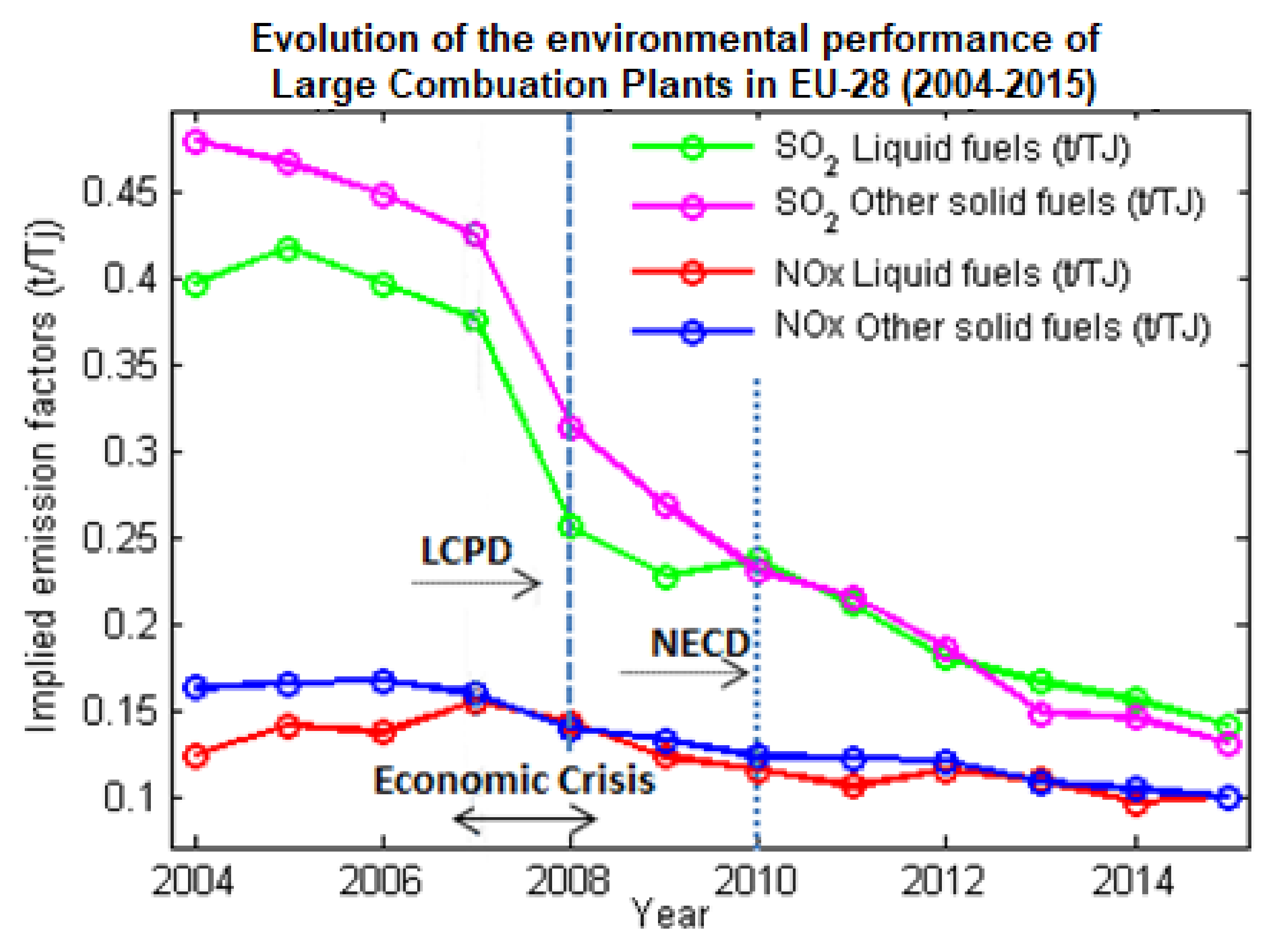
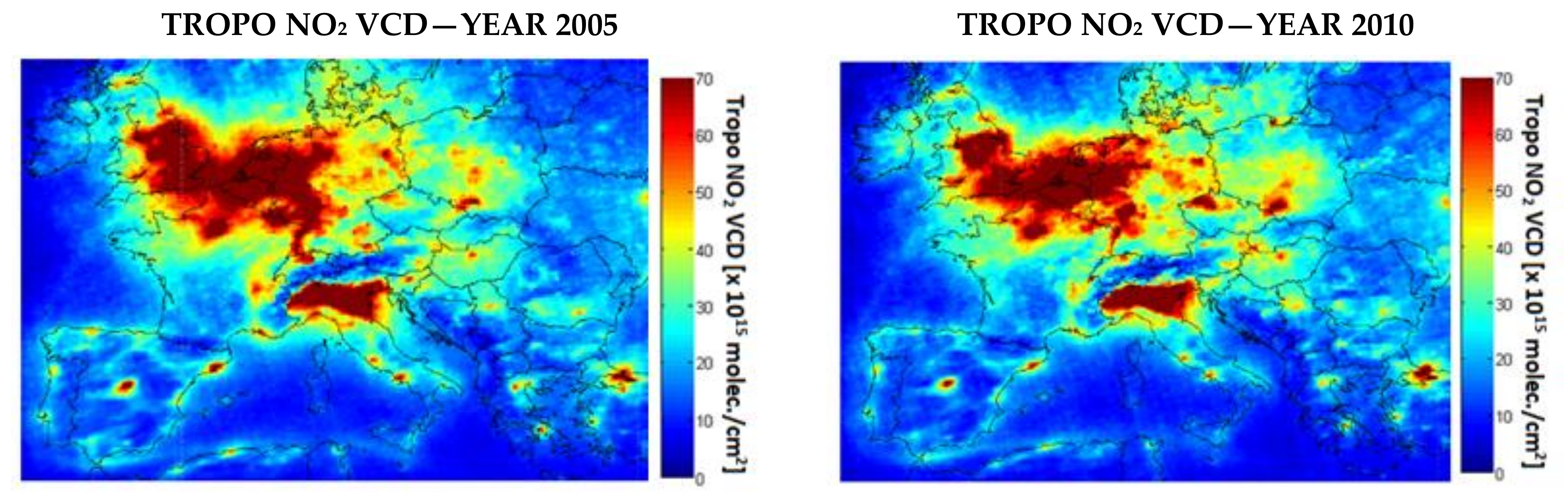
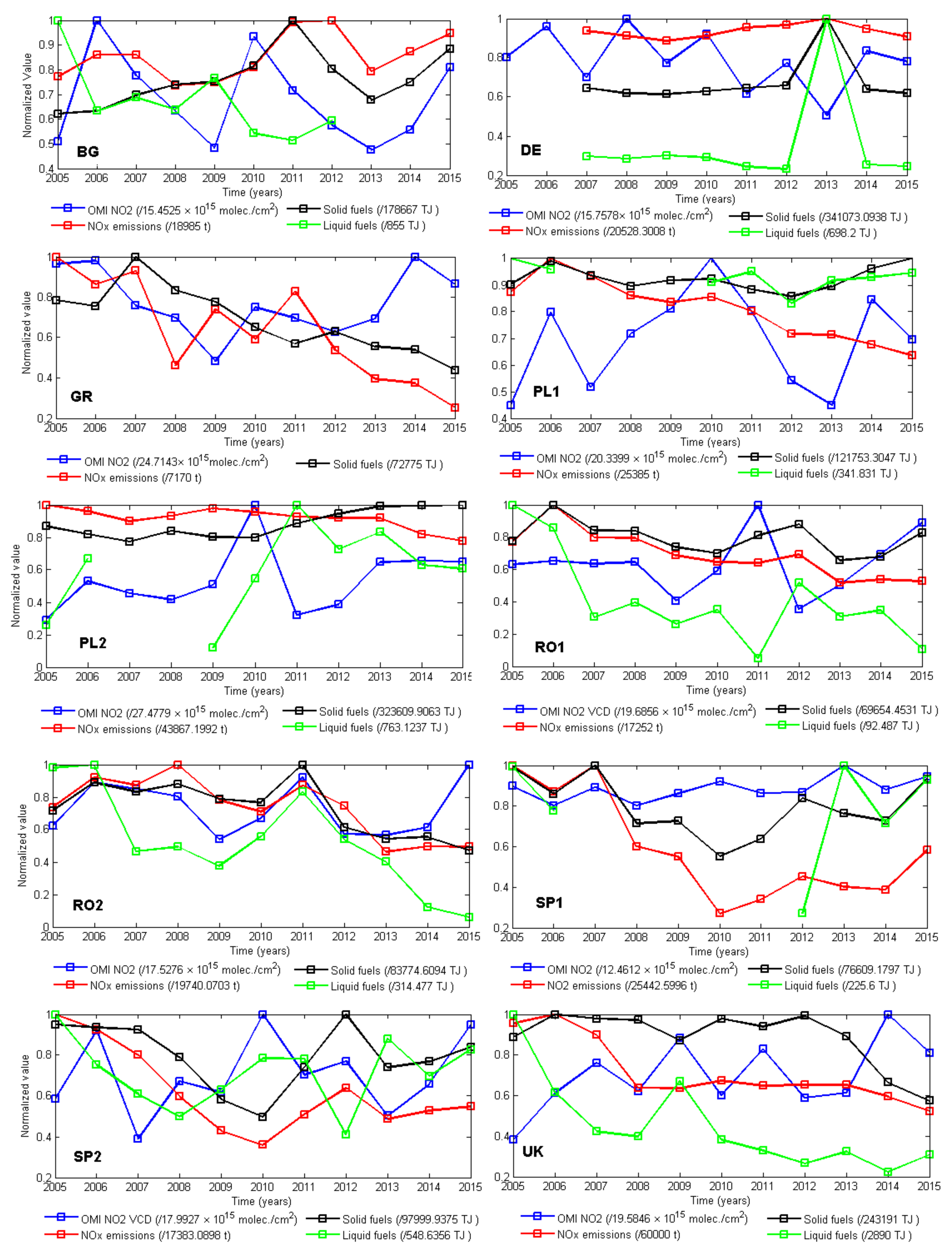
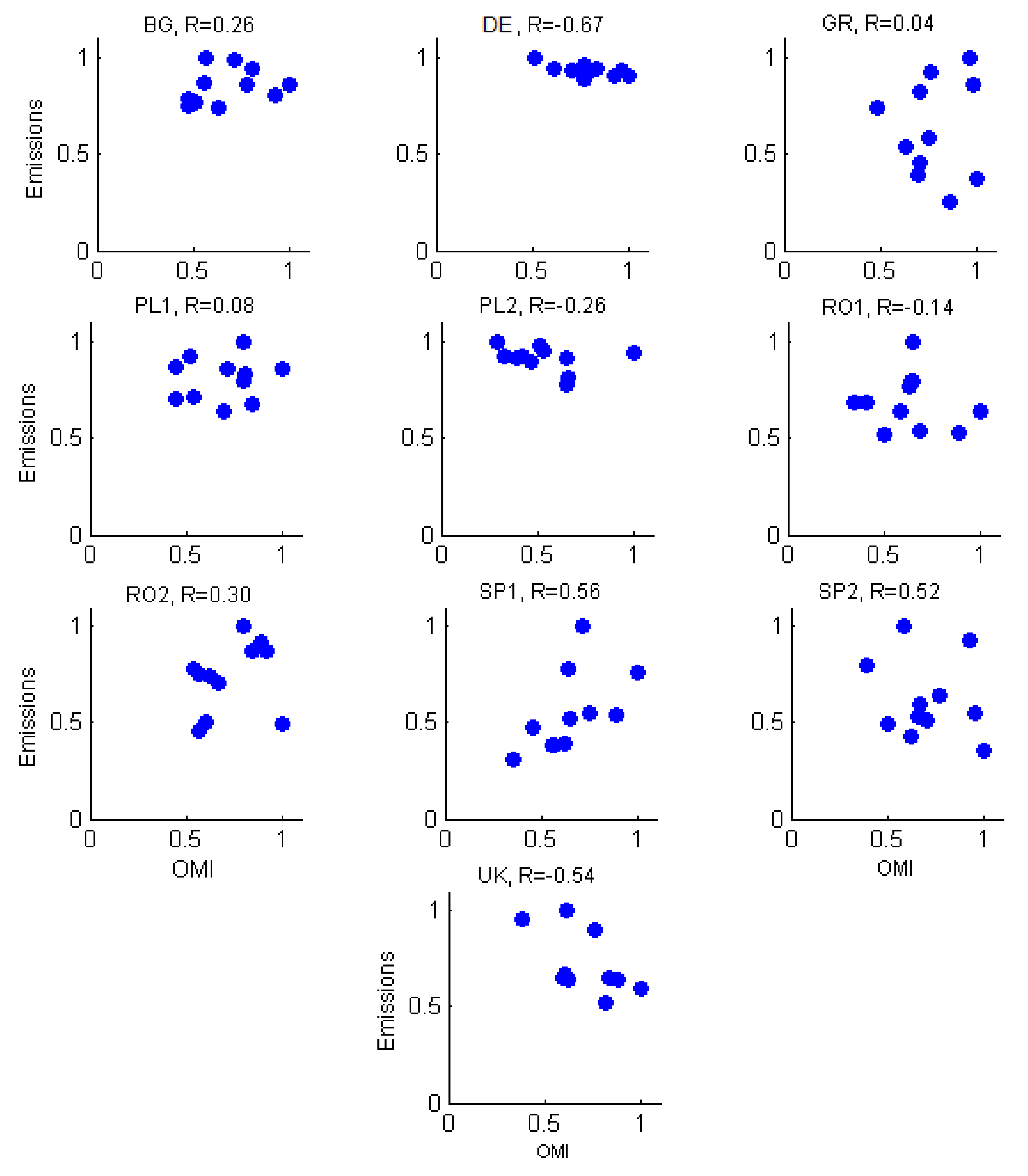
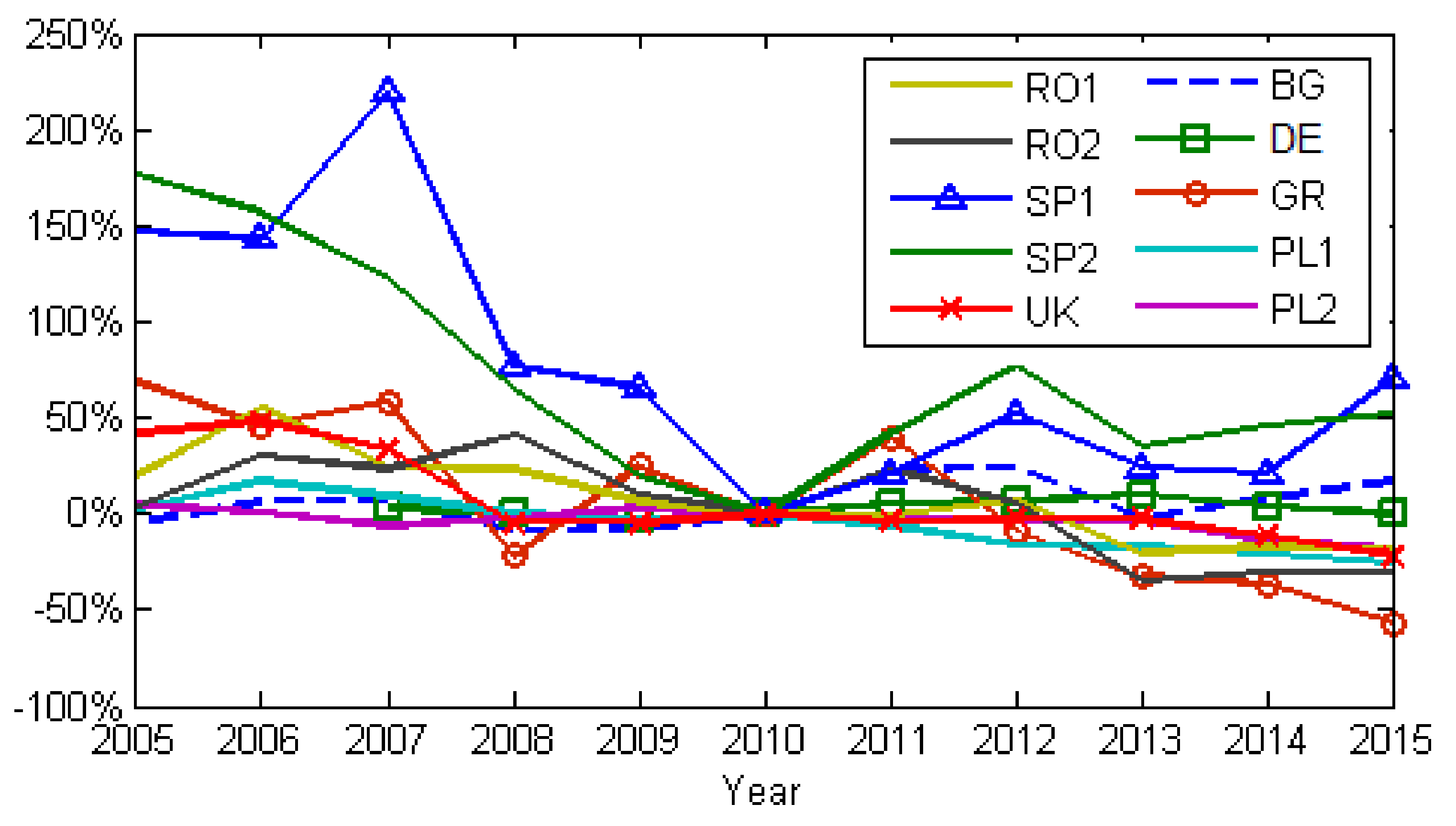
3.1. Nitrogen Oxides
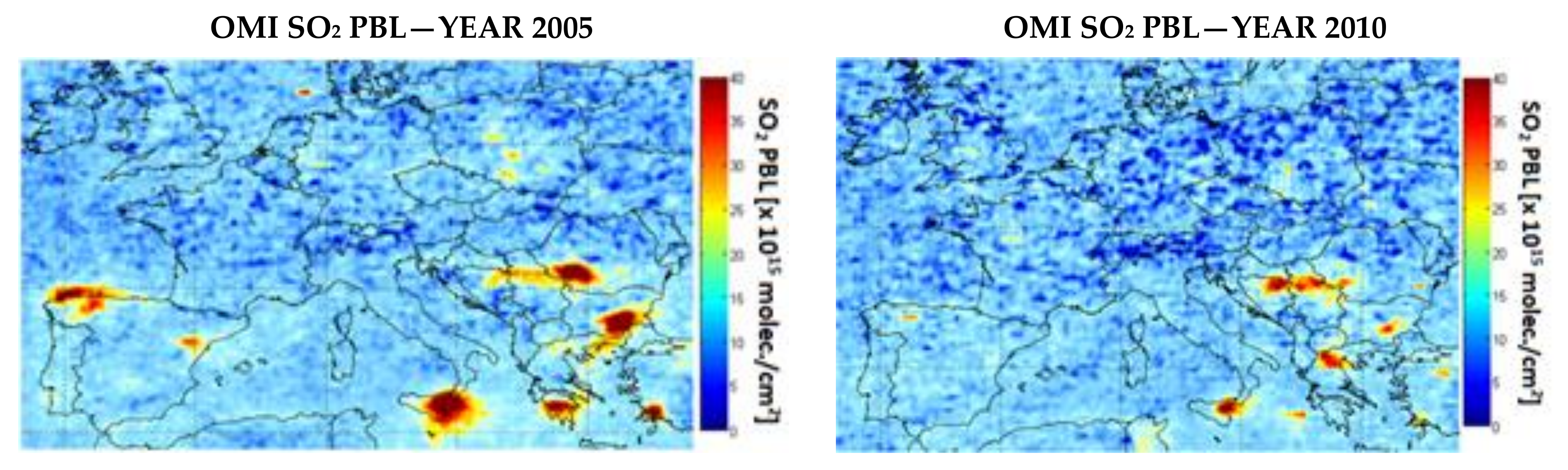
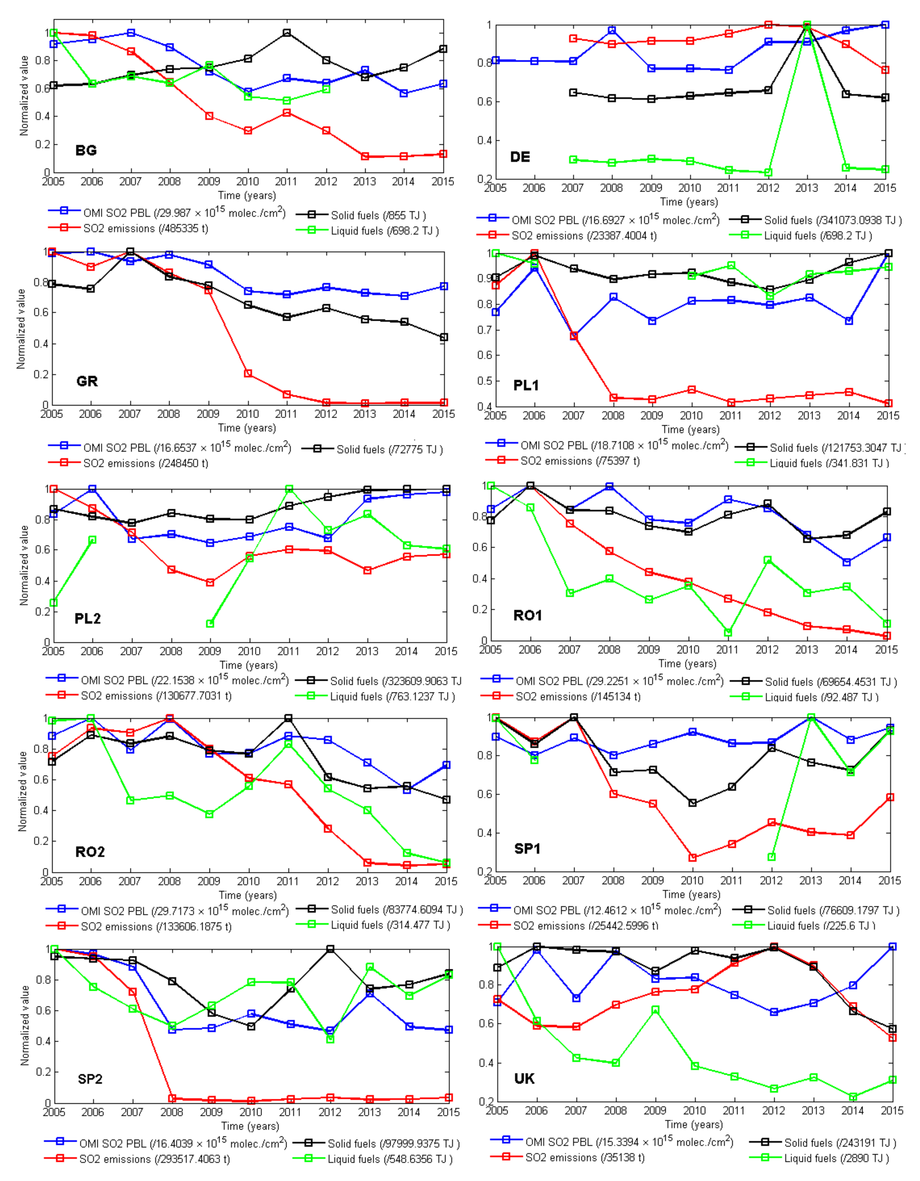
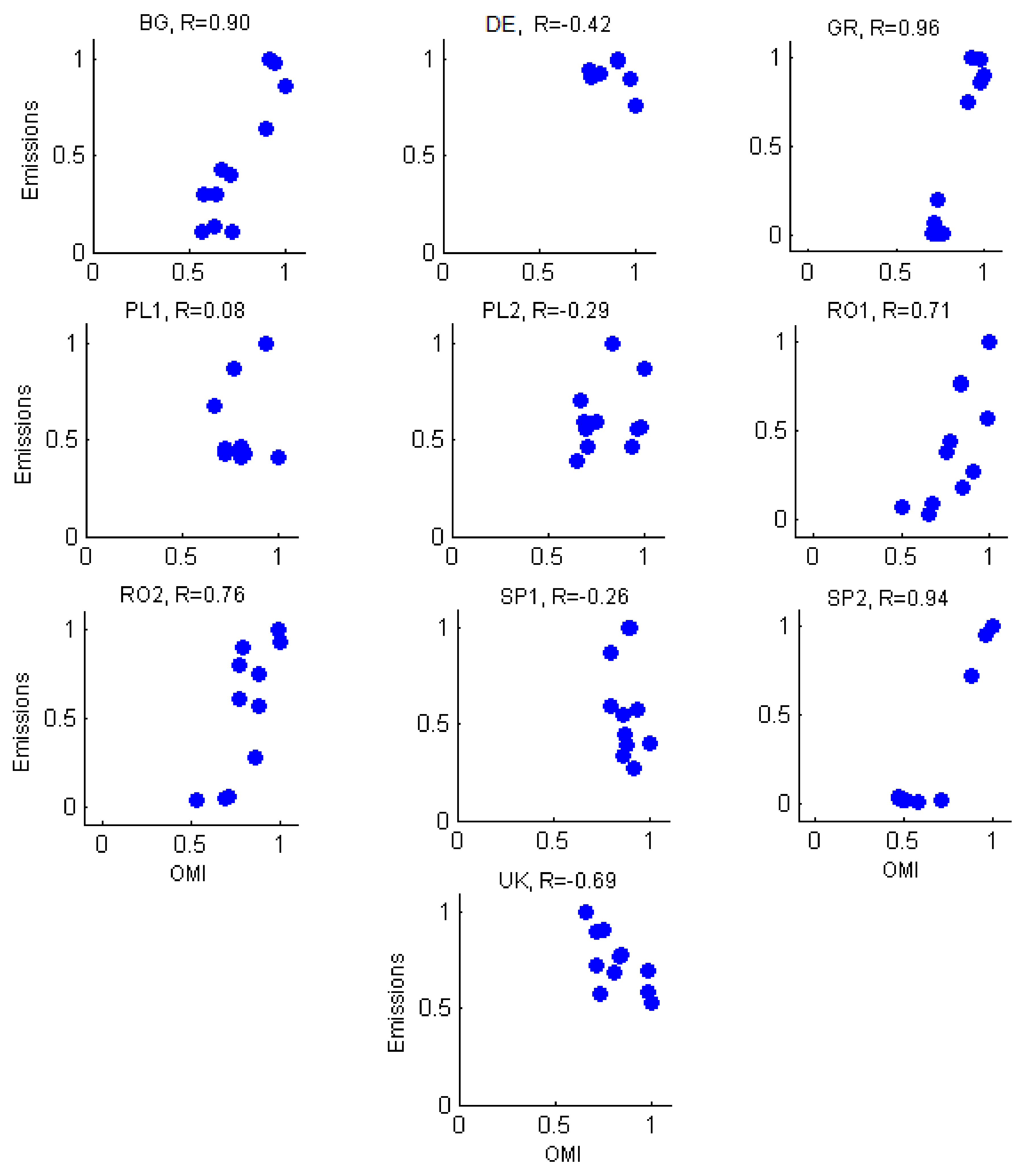
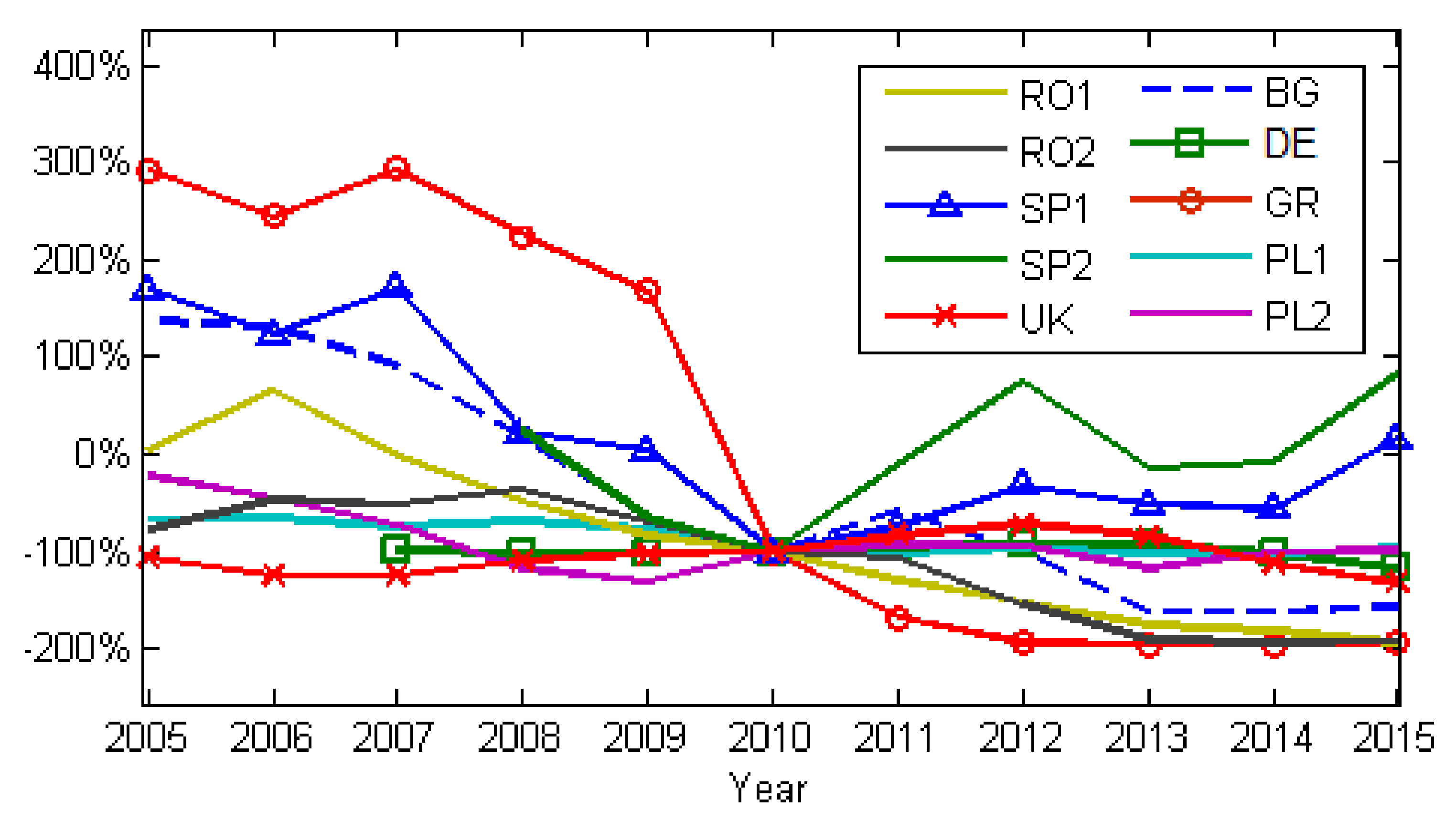
Figure 5 shows the NO2 evolution for each power plant, during 2005–2015, resulting from OMI measurements of the tropospheric NO2VCDs and from estimated emissions. The latter are reported by each EU country to the EEA. Plots include the consumption of liquid and solid fuels per LCP. All measurements are normalized to their maximum. Expectedly, emission calculations follow roughly the trend of solid/liquid consumption, since the calculation of the former are based on the latter.
Almost all reported emissions of NO2 showed a decreasing trend, except plants in BG and DE, while OMI space observations show an increasing trend for all, except plants in BG and GR. Note that one cannot expect a one-to-one correspondence between the reported emissions and space observations. On the one hand, differences between emissions and OMI stem from the fact that the satellite instrument sees a large area (13 km × 24 km), thus measurements contain background NO2 and the NO2 released by surrounding local/traffic sources. Secondly, satellite results are subject to various assumptions related to the atmospheric mass factor (AMF) calculations. The emissions, on the other hand, are based on calculations based on the quantity and nature of fossil fuel. The type and quality of fuel may influence the quantity of emissions, the correlation between the quantity of calculated emissions, and the nature of the fossil fuel (solid or liquid) which could give the main fuel used during the thermal processes. The discrepancies may also be due to the fact that OMI soundings are done at a specific time (i.e., the overpass time), which is associated with various phases of the diurnal variation of NO2, depending on the geographical location of the station.
OMI measurements and estimated emissions correlate fairly well (R >0.5) for a few power plants: BG, RO2, and SP1. However, for the other plants, there is practically no correlation since minima and maxima in the two-time series are even opposing (e.g., SP2, DE, and GR). A clear peak is seen in the NO2 satellite time series around 2010–2011, when the winter was unusually cold in Europe [40], for all stations except stations GR, SP1, and the UK. The first are the southernmost ones, which probably were less affected by the low temperatures, while the UK had a different climate compared to the continent. The increased NO2 concentration may be the result of a combination of the increased request for heating and a higher lifetime of NO2, of the order of days, when temperatures are low. An important characteristic of the NO2 evolution, very well highlighted in OMI space observations, was the global financial and economic crisis during 2007–2009 [26,41,42,43]. Considering the influence of the financial and economic crisis (2007–2009) on the emissions, the end of recessions could correspond to the emissions increase in 2010 and after this year.
Scatter plots of OMI measurements against the reported emission for NO2 amount are shown in Figure 6, for all plants. Satellite measurements seemed to be a good indicator for emission variability only for some LCPs: EP1, EP2, BG, and RO2, for which correlation coefficients were positive (R = 0.56, 0.52, 0.26, 0.32). For other plants, the emissions varied in a completely different manner than the satellite measurements of tropoVCDs. Low emissions corresponded to high values of satellite VCDs of NO2 and vice versa. Large negative correlations between the two datasets were seen, e.g., in the UK (R = −0.54) or DE (R = −0.67). Indeed, as mentioned before, satellite data will inevitably contain also the background NO2 resulting from all sources in an area of about 300 km2. VCDs also respond to background conditions (higher or lower temperatures, wind effect, urban agglomeration), while emissions relate only to fuel consumption. For LCPs where OMI showed an increasing trend while the calculated emissions show the opposite, the explanation could be the fact that the calculated emissions from LCP do not include the nearby emissions, as urban and traffic emissions, or other industries; the latter are however included in space observations. This may be the case since Figure 5 shows that towards the end of the selected period, most emissions decreased, while tropospheric VCDs increased. However, the very large differences seen for other stations cannot be explained.

3.2. Sulfur Dioxide

The SO2 emissions of power plants in Europe have drastically decreased over the last 20 years. Figure 7 shows that during 2005–2015, the observed SO2 observed by OMI (blue line) has no trend (as in PL1, PL2, SP1, and the UK) or is slightly decreasing (BG, GR, RO1, EO2, and SP2). The emissions (red line), on the other hand, have a clear decreasing trend for most stations, except the UK, with a maximum in 2012, and DE, where the highest emissions were reported also in 2012.
Similar to NO2, we do not aim to compare satellite measurements, emission, and fuel consumption, but their annual variation (this is also why we use normalized values). The similarities between satellite data and emissions are better for SO2 than for NO2. Some discrepancies between the two-time series were seen for the UK, PL1, or DE. Emissions decreased more abruptly than to VCD measurements in GR, PL1, RO2, RO1, SP2, and SP1. Even if the trend was the same, differences between the relative variations of VCDs and emissions were still high (e.g., GR, PL1, RO1, and SP2) (Figure 7). Important factors to be considered are (1) the overpass time of the space sensor over the emission source and, as in the case of NO2, and (2) the contribution of other sources to the SO2 amount measured by satellite. Except for the two plants from Spain (SP1 and SP2), SO2 emissions decreased, on average, after 2010. Satellite measurements confirmed the SO2 decrease, especially for BG and GR. The descending trend of reported SO2 emissions was higher compared to the descending trend of SO2 observed from space. The correlation between the SO2 content observed from space and the type of fossil fuel may indicate whether the main used fuel is liquid or solid.
The large difference between the trend of reported emissions and space observations over the power plants from Greece, Romania, and Spain can be explained by the use of improved SO2 filter systems, e.g., the case of Romanian LCPs [44,45].
Figure 8 confirms that SO2 satellite measurements correlated better to the corresponding emissions compared to NO2 for BG, GR, PL2, RO1, RO2, and SP2. The variation of SO2 emissions of the UK, DE, PL1, and SP1 were not supported by satellite measurements of tropospheric column. Similar to the analysis of NO2, satellite measurements average over a larger area and include background or transport emissions.
A slight decrease was seen in the satellite-based SO2 for BG, GR, RO1, RO2, and SP2. For the rest (SP1, DE, and the UK), no clear trend could be identified.
A good correlation was at PL2, RO1, RO2, and BG, where at least there were no large discrepancies between the annual variations, and decreased emissions were, most times, supported by accompanying decreases in SO2 measurements. A good correlation between the two sets was also seen at the DE station, where, despite the small value of the correlation coefficient, both satellite and estimated emissions showed a similar variation of the SO2 content.
A different variation was seen for emissions at GR, PL1, RO1, and RO2, which went down to 40% of their initial values in 2005, 2006, and 2007. This decrease, however, was not backed up by satellite measurements whose variation is (as for the UK) about 25% of the maximum. Something marginally similar was seen in SP2 and GR, where the decrease in emissions after 2008 was even more dramatic, going down by almost 90%. Satellite measurements partly supported, in general, the decrease in SO2, even if the corresponding variation was only 30%–50%. This discrepancy can be explained by possible additional SO2 loading seized by the satellite instrument. However, natural sources of SO2 cannot account for the difference, and most SO2 originated from coal and oil burning, unlike NO2.
For the UK, the situation is completely different, since both emissions and measurements vary within the same range, but they are anticorrelated. The effects of the cold winter of 2010 and the financial and economic crisis on the SO2 variability were less visible than for NO2. This may have been related to the fact that the power plants had improved their SO2 filtering system, the burning system and the quality of the fuel used, e.g., this would be the case of Romanian power plants, for which the implementation of the EU directives was achieved gradually during 2007–2013 [28]. This was seen both in satellite measurements and in the emissions for stations in Romania (RO1 and RO2).
Some inconsistencies between space observations and ground emissions may also arise from the electricity demand or the energy consumption curve, which is represented by the electricity demand function of time. The space sensor can have the overpass time during high demand of electricity, which corresponds to high emissions. OMI passes over the Romanian LCP around 10–12 UTC, which corresponds to the time interval of high demand for electricity [46]. In such a case, i.e., when the overpass time of the space sensor coincides with a high demand of energy, thus of SO2, this may explain the fact that the satellite-based SO2 may overestimates the SO2 emissions. The reported emissions are based on daily emissions calculations while the space observations are based-on one, two, or no observation per day function of orbit. Note that the EU Directives does not impose hourly or daily limits for the emissions, the emission restrictions are quantified annually.
Figure 9 and Figure 10 show the annual changes in emissions relative to 2010, for NOx and SO2. We chose 2010 because, by then, the level of national emissions, including those caused by LCPs, should have complied with the NEC Directive (2001/81/EC). According to Figure 5 and Figure 7, emissions for all LCPs presented in this work show descending trends until 2010. After 2010 a clear increasing trend for both NOx and SO2 emissions was observed only for power plants in Spain. The NOx and SO2 emissions descending trend was the result of the EU Directives, combined with the financial and economic crisis during 2007–2009. Figure 11 shows the influence of the financial and economic crisis on the evolution of the Nominal GDP (Gross Domestic Product) and electrical energy production using fossil fuels during 2005–2015 (Eurostat, https://ec.europa.eu/eurostat/data/database).

4. Conclusions

In this paper, we presented the variation of NO2 and SO2 atmospheric emissions attributed to ten very large power plants across Europe (EU-28), quantified by calculated emissions and by satellite observations, during 2005–2015. The main aim of this work was to study the evolution of the NO2 and SO2 amount after implementation of the LCP Directive (2001/80/EC), and the NEC Directive (2001/81/EC). Another goal of the comparison was to see to what extent changes in reported emissions to EEA by each country are supported by OMI space-based observations. We presented that OMI observations support the changes in reported emissions to EEA by the EU-28 countries. We identified most of the main drivers for the emissions decrease or increase during 2005–2015. We found that the financial and economic crisis during 2007–2009 had an important role in the emission reduction before 2010.
In general, the NO2 and SO2 emissions from LCPs in the Eastern European countries were larger than for Western European countries. During the period between 2005 and 2015, some Eastern Europe socio-political changes triggered by the accession to the European Union took place, requiring compliance with the legislation imposing pollution limits. These changes were directly reflected in the corresponding emission reductions of NO2 and SO2. The reduction in solid fuel consumption (in both Eastern and Western Europe) was balanced by the growth of gas consumption or by renewable and nuclear energy [47]. In Eastern Europe, OMI showed a substantial SO2 reduction in the proximity of the coal-fired power plants, because flue-gas desulfurization equipment was installed during the study period.
The satellite observations clearly detected a decreasing tendency of NO2 and SO2 amount for the entire analyzed period. The satellite observations presented in this paper support the conclusion about the recent decline in NOx and SO2 emissions from power plants across Europe, where the EU policies for emission reduction played a key role in the LCP emissions reduction. Future work will focus on the impact assessment of the Industrial Emissions Directive (IED) over the LCPs presented in this study.

Author Contributions

Conceptualization, D.-E.C. and M.A.; formal analysis, D.-E.C. and M.V.; investigation, C.B., D.-E.C., and M.V.; methodology, C.B.; validation, D.-E.C.; writing–original draft, D.-E.C. and M.V.; writing– review and editing, D.-E.C., M.V., A.M., M.V.R., A.R., and P.L.G. All authors have read and agreed to the published version of the manuscript.

Funding

The work of D.-E.C., M.V., and P.L.G. was supported by the project “EXPERT”, financed by the Romanian Ministry of Research and Innovation, Contract no. 14PFE/17.10.2018, while the work of A.R. was supported by the project ANTREPRENORDOC, in the framework of Human Resources Development Operational Programme 2014–2020, financed from the European Social Fund, under the contract number 36355/23.05.2019 HRD OP/380/6/13—SMIS Code: 123847.

Acknowledgments

SO2 analyses and visualizations used in this paper were produced with the Giovanni online data system, developed and maintained by the NASA GES DISC via https://giovanni.gsfc.nasa.gov. Also, the authors are grateful for the free use of tropospheric NO2 and data from the OMI sensor via http://www.temis.nl. SO2 and NOx emissions were obtained from the European Environment Agency via https://www.eea.europa.eu/data-and-maps/data/lcp-9).

Conflicts of Interest

The authors declare no conflict of interest.

References

  1. European Environment Agency. Air Quality in Europe—2015 Report; EEA Report No 5/2015; European Environment Agency: Copenhagen, Denmark, 2015. [Google Scholar]
  2. European Environment Agency. European Union Emission Inventory Report 1990–2016 under the UNECE Convention on Long-Range Transboundary Air Pollution (LRTAP); EEA Report 2016, No.6/2018; European Environment Agency: Copenhagen, Denmark, 2018. [Google Scholar]
  3. Maître, A.; Bonneterre, V.; Huillard, L.; Sabatier, P.; de Gaudemaris, R. Impact of urban atmospheric pollution on coronary disease. Eur. Heart J. 2006, 27, 2275–2284. [Google Scholar] [CrossRef] [PubMed] [Green Version]
  4. Makri, A.; Stilianakis, N.I. Vulnerability to Air Pollution Health Effects. Int. J. Hyg. Environ. Health 2008, 211, 326–336. [Google Scholar] [CrossRef] [PubMed]
  5. Witek, T.J.; Schachter, E.N.; Beck, G.J.; Cain, W.S.; Colice, G.; Leaderer, B.P. Respiratory symptoms associated with sulfur dioxide exposure. Int. Arch. Occup. Environ. Health 1985, 55, 179–183. [Google Scholar] [CrossRef] [PubMed]
  6. Singh, A.; Agrawal, M. Acid rain and its ecological consequences. J. Environ. Biol. 2007, 29, 15. [Google Scholar]
  7. Rosu, A.; Constantin, D.E.; Georgescu, L. Air pollution level in Europe caused by energy consumption and transportation. J. Environ. Prot. Ecol. 2016, 17, 1–8. [Google Scholar]
  8. EU. Directive 2001/80/EC of the European Parliament and of the Council of 23 October 2001 on the Limitation of Emissions of Certain Pollutants into the Air from Large Combustion Plants; EU: Brussels, Belgium, 2001. [Google Scholar]
  9. EU. Directive 2008/1/EC of the European Parliament and of the Council of 15 January 2008 Concerning Integrated Pollution Prevention and Control; EU: Brussels, Belgium, 2008. [Google Scholar]
  10. EU. Directive 2001/81/EC of the European Parliament and of the Council of 23 October 2001 on National Emission Ceilings for Certain Atmospheric Pollutants; EU: Brussels, Belgium, 2001. [Google Scholar]
  11. EU. Directive 2010/75/EU of the European Parliament and of the Council of 24 November 2010 on Industrial Emissions (Integrated Pollution Prevention and Control); EU: Brussels, Belgium, 2010. [Google Scholar]
  12. Constantin, D.E.; Merlaud, A.; Voiculescu, M.; Van Roozendael, M.; Arseni, M.; Rosu, A.; Georgescu, L. NO2 and SO2 observations in southeast Europe using mobile DOAS observations. Carpathian J. Earth Environ. Sci. 2017, 12, 323–328. [Google Scholar]
  13. Yang, J.; Gong, P.; Fu, R.; Zhang, M.; Chen, J.; Liang, S.; Dickinson, R. The role of satellite remote sensing in climate change studies. Nat. Clim. Chang. 2013, 3, 875. [Google Scholar] [CrossRef]
  14. Eisinger, M.; Burrows, J.P. Tropospheric sulfur dioxide observed by the ERS-2 GOME instrument. Geophys. Res. Lett. 1998, 25, 4177–4180. [Google Scholar] [CrossRef] [Green Version]
  15. Burrows, J.P.; Weber, M.; Buchwitz, M.; Rozanov, V.; Ladstätter-Weißenmayer, A.; Richter, A.; DeBeek, R.; Hoogen, R.; Bramstedt, K.; Eichmann, K.-U.; et al. The Global Ozone Monitoring Experiment (GOME): Mission Concept and First Scientific Results. J. Atmos. Sci. 1999, 56, 151–175. [Google Scholar] [CrossRef]
  16. Constantin, D.-E.; Voiculescu, M.; Georgescu, L. Satellite Observations of NO2 Trend over Romania. Sci. World J. 2013, 2013. [Google Scholar] [CrossRef]
  17. Paraschiv, S.; Constantin, D.-E.; Paraschiv, S.-L.; Voiculescu, M. OMI and Ground-Based In-Situ Tropospheric Nitrogen Dioxide Observations over Several Important European Cities during 2005–2014. Int. J. Environ. Res. Public Health 2017, 14, 1415. [Google Scholar] [CrossRef] [PubMed] [Green Version]
  18. Rosu, A.; Rosu, B.; Constantin, D.E.; Arseni, M.; Voiculescu, M.; Georgescu, L.P.; Popa, I. Overview of tropospheric NO2 using the ozone monitoring observations instrument and human perception about air quality for the most polluting countries accross the world. Carpathian J. Earth Environ. Sci. 2019, 14, 423–430. [Google Scholar]
  19. Levelt, P.; van den Oord, G.; Dobber, M.; Malkki, A.; Visser, H.; de Vries, J.; Stammes, P.; Lundell, J.; Saari, H. The ozone monitoring instrument. IEEE Trans. Geosci. Remote 2006, 44, 1093–1101. [Google Scholar] [CrossRef]
  20. Fioletov, V.E.; McLinden, C.A.; Krotkov, N.; Li, C. Lifetimes and emissions of SO2 from point sources estimated from OMI. Geophys. Res. Lett. 2015, 42, 1969–1976. [Google Scholar] [CrossRef]
  21. Lin, J.; McElroy, M.B.; Boersma, F. Constraint of anthropogenic NOx emissions in China from different sectors: A new methodology using multiple satellite retrievals. Atmos. Chem. Phys. Discuss. 2010, 10, 63–78. [Google Scholar] [CrossRef] [Green Version]
  22. Wang, S.; Streets, D.G.; Zhang, Q.; He, K.; Chen, D.; Kang, S.; Wang, Y. Satellite detection and model verification of NO x emissions from power plants in Northern China. Environ. Res. Lett. 2010, 5, 044007. [Google Scholar] [CrossRef]
  23. Kim, S.-W.; Heckel, A.; McKeen, S.A.; Frost, G.J.; Hsie, E.-Y.; Trainer, M.K.; Grell, G.A. Satellite-observed U.S. power plant NO x emission reductions and their impact on air quality. Geophys. Res. Lett. 2006, 33, L22812. [Google Scholar] [CrossRef] [Green Version]
  24. Van der A, R.J.; Mijling, B.; Ding, J.; Koukouli, M.E.; Liu, F.; Li, Q.; Mao, H.; Theys, N. Cleaning up the air: Effectiveness of air quality policy for SO2 and NOx emissions in China. Atmos. Chem. Phys. 2017, 17, 1775–1789. [Google Scholar] [CrossRef] [Green Version]
  25. Wang, T.; Wang, P.; Theys, N.; Tong, D.; Hendrick, F.; Zhang, Q.; Van Roozendael, M. Spatial and temporal changes in SO2 regimes over China in the recent decade and the driving mechanism. Atmos. Chem. Phys. 2018, 18, 18063–18078. [Google Scholar] [CrossRef] [Green Version]
  26. Russell, A.R.; Valin, L.C.; Cohen, R.C. Trends in OMI NO2 observations over the United States: Effects of emission control technology and the economic recession. Atmos. Chem. Phys. 2012, 12, 12197–12209. [Google Scholar] [CrossRef] [Green Version]
  27. De Foy, B.; Lu, Z.; Streets, D.G.; Lamsal, L.N.; Duncan, B.N. Estimates of power plant NOx emissions and lifetimes from OMI NO2 satellite retrievals. Atmos. Environ. 2015, 116, 1–11. [Google Scholar] [CrossRef]
  28. Krotkov, N.A.; McLinden, C.A.; Li, C.; Lamsal, L.N.; Celarier, E.A.; Marchenko, S.V.; Swartz, W.H.; Bucsela, E.J.; Joiner, J.; Duncan, B.N.; et al. Aura OMI observations of regional SO2 and NO2 pollution changes from 2005 to 2015. Atmos. Chem. Phys. 2016, 16, 4605–4629. [Google Scholar] [CrossRef] [Green Version]
  29. Li, C.; McLinden, C.; Fioletov, V.; Krotkov, N.; Carn, S.; Joiner, J.; Dickerson, R.R. India is overtaking China as the world’s largest emitter of anthropogenic sulfur dioxide. Sci. Rep. 2017, 7, 14304. [Google Scholar] [CrossRef] [PubMed] [Green Version]
  30. EU. Assessing the Effectiveness of EU Policy on Large Combustion Plants in Reducing Air Pollutant Emissions; EEA Report No 07/2019; EU: Brussels, Belgium, 2019; ISSN 1977-8449. [Google Scholar] [CrossRef]
  31. EU. Emissions of Air Pollutants from Large Combustion Plants, Indicator Assessment; Prod-ID: IND-427-en(a); EU: Brussels, Belgium, 2017; Available online: https://www.eea.europa.eu/data-and-maps/indicators/emissions-of-air-pollutants-from/assessment-1 (accessed on 15 April 2020).
  32. EU. Emissions of air Pollutants from Large Combustion Plants in Europe, Indicator Assessment; Prod-ID: IND-427-en(b); EU: Brussels, Belgium, 2020; Available online: https://www.eea.europa.eu/data-and-maps/indicators/emissions-of-air-pollutants-from-16/assessment (accessed on 15 April 2020).
  33. Singhal, P. Are Emission Performance Standards Effective in Pollution Control? Evidence from the EU’s Large Combustion Plant Directive; DIW Berlin: Berlin, Germany, 2019; Discussion Paper No. 1773; Available online: https://ssrn.com/abstract=3297528 (accessed on 1 June 2019). [CrossRef] [Green Version]
  34. Meyer, A.; Pac, G. Analyzing the characteristics of plants choosing to opt-out of the Large Combustion Plant Directive. Util. Policy 2017, 45, 61–68. [Google Scholar] [CrossRef] [Green Version]
  35. Boersma, K.F.; Eskes, H.J.; Dirksen, R.J.; van der A, R.J.; Veefkind, J.P.; Stammes, P.; Huijnen, V.; Kleipool, Q.L.; Sneep, M.; Claas, J.; et al. An improved retrieval of tropospheric NO2 columns from the Ozone Monitoring Instrument. Atmos. Meas. Tech. 2011, 4, 1905–1928. [Google Scholar] [CrossRef] [Green Version]
  36. Acker, J.G.; Leptoukh, G. Online Analysis Enhances Use of NASA Earth Science Data. Eos Trans. AGU 2007, 88, 14–17. [Google Scholar] [CrossRef]
  37. Li, C.; Joiner, J.; Krotkov, N.A.; Bhartia, P.K. A fast and sensitive new satellite SO2 retrieval algorithm based on principal component analysis: Application to the Ozone Monitoring Instrument. Geophys. Res. Lett. 2013. [Google Scholar] [CrossRef] [Green Version]
  38. Krotkov, N.A.; Carn, S.A.; Krueger, A.J.; Bhartia, P.K.; Yang, K. Band residual difference algorithm for retrieval of SO2 from the Aura Ozone Monitoring Instrument (OMI). IEEE Trans. Geosci. Remote Sens. 2006, 44, 1259–1266. [Google Scholar] [CrossRef]
  39. Nickolay, A.; Krotkov, C.L.; Leonard, P. OMI/Aura Sulfur Dioxide (SO2) Total Column L3 1 Day Best Pixel in 0.25 Degree x 0.25 Degree V3; Goddard Earth Sciences Data and Information Services Center (GES DISC): Greenbelt, MD, USA, 2015. [Google Scholar] [CrossRef]
  40. Cattiaux, J.; Vautard, R.; Cassou, C.; Yiou, P.; Masson-Delmotte, V.; Codron, F. Winter 2010 in Europe: A cold extreme in a warming climate. Geophys. Res. Lett. 2010, 37. [Google Scholar] [CrossRef] [Green Version]
  41. Castellanos, P.; Boersma, K.F. Reductions in nitrogen oxides over Europe driven by environmental policy and economic recession. Sci. Rep. 2012, 2, 1–7. [Google Scholar] [CrossRef]
  42. Liu, F.; Zhang, Q.; Zheng, B.; Tong, D.; Yan, L.; Zheng, Y.; He, K. Recent reduction in NOx emissions over China: Synthesis of satellite observations and emission inventories. Environ. Res. Lett. 2016, 11, 114002. [Google Scholar] [CrossRef] [Green Version]
  43. Vrekoussis, M.; Richter, A.; Hilboll, A.; Burrows, J.P.; Gerasopoulos, E.; Lelieveld, J.; Barrie, L.; Zerefos, C.; Mihalopoulos, N. Economic crisis detected from space: Air quality observations over Athens/Greece. Geophys. Res. Lett. 2013, 40, 458–463. [Google Scholar] [CrossRef]
  44. ANPM. Air Quality Management Program of Gorj County 2010–2013. Available online: www.anpm.ro/anpm_resources/migrated_content/uploads/20817_Program%20CA%20jud_Gorj.pdf (accessed on 12 June 2017).
  45. Merlaud, A.; Belegante, L.; Constantin, D.-E.; Den Hoed, M.; Meier, A.C.; Allaart, M.; Ardelean, M.; Arseni, M.; Bösch, T.; Brenot, H.; et al. The Airborne ROmanian Measurements of Aerosols and Trace gases (AROMAT) campaigns. Atmos. Meas. Tech. Discuss. 2020. in review. [Google Scholar] [CrossRef]
  46. Bogdan, M.; Stanescu, D.; Stanescu, C.; Achim, N. Aspecte didactice privind contorul inteligent de energie electrică. In Proceedings of the Simpozionul International “Contorizare Inteligenta”, Sibiu, Romania, 14–17 November 2017. [Google Scholar]
  47. Vestreng, V.; Myhre, G.; Fagerli, H.; Reis, S.; Tarrasón, L. Twenty-five years of continuous sulphur dioxide emission reduction in Europe. Atmos. Chem. Phys. 2007, 7, 3663–3681. [Google Scholar] [CrossRef] [Green Version]
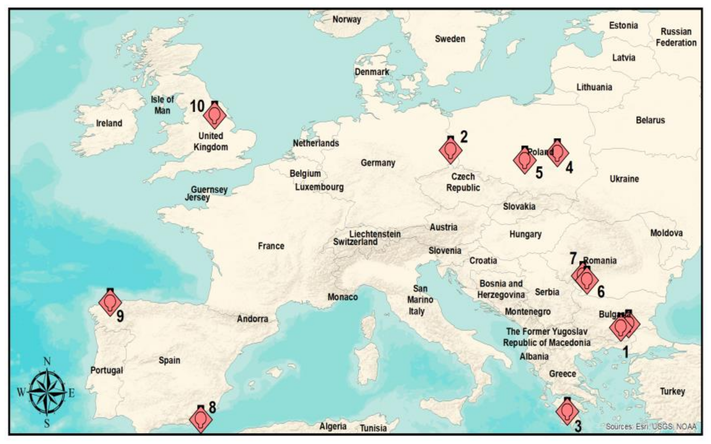
Figure 1. Evolution of the environmental performance of large combustion plants in the EU-28, expressed as implied emission factors for SO2 and NOx by fuel type.
Ijerph 17 03630 g001
Figure 2. The spatial distribution of LCPs; these are identified by the corresponding numbers in Table 1.
Ijerph 17 03630 g002
Figure 3. Annual tropospheric NO2 VCD based on OMI observations for 2005 vs. 2010.
Ijerph 17 03630 g003
Figure 4. Annual tropospheric SO2 PBL based on OMI observations for 2005 vs. 2010.
Ijerph 17 03630 g004
Figure 5. Time series of normalized NO2 during 2005–2015 using data from satellite instruments (blue) and emissions (red) for each station, together with the reported solid fuel (black) and liquid fuel consumption (green).
Ijerph 17 03630 g005
Figure 6. Scatter plots of OMI measurements vs. reported emission for NO2 (normalized values).
Ijerph 17 03630 g006
Figure 7. Time series of normalized SO2 during 2005–2015 using data from satellite instruments (blue) and emissions (red), together with the reported solid fuel (black) and liquid fuel consumption (green).
Ijerph 17 03630 g007
Figure 8. Scatter plots of OMI measurements vs. emissions for SO2 (normalized values).
Ijerph 17 03630 g008
Figure 9. Changes in NOx emissions relative to 2010, the milestone being NEC Directive.
Ijerph 17 03630 g009
Figure 10. Changes in SO2 emissions relative to 2010, the milestone being NEC Directive.
Ijerph 17 03630 g010
Figure 11. Comparison between Nominal GDP and Electrical Energy over the EU during 2005–2015, where TOE represents a tonne of oil equivalent (source: Eurostat).
Ijerph 17 03630 g011
Table 1. Information for individual power plants (source: EEA *).
Power PlantCountryCodeLat. (°)Long. (°)Average
Annual
Power
(MWth)
Average Annual
SO2
Emissions (T)
Average Annual
NOX
Emissios (t)
1. TPP “Maritsa Iztok 2”
TPP “Maritsa Iztok 3”
Stara Zagora
BulgariaBG42.25
42.05
26.13
25.62
6743232,08416,211
2. KW Jänschwalde, PeitzGermanyDE51.8314.46914421,43819,218
3. PPC S.A.–Megalopoli I-IVGreeceGR37.4122.102381108,6204543.5
4. Elektrownia “Kozienice” S.A.PolandPL151.6621.467023.141,33420,544
5. PGE Górnictwo i Energetyka Konwencjonalna S.A.–Oddział Elektrownia Bełchatów, Łódź VoivodeshipPolandPL251.2619.331317080,78940,217
6. S.C. Complexul Energetic Oltenia S.A., Rovinari 1-2RomaniaRO144.9023.13351260,16611,937
7. S.C. Complexul Energetic Turceni S.A. 1-4RomaniaRO244.6623.41473472,82414,526
8. CT LITORAL I-II, Carboneras-AlmeriaSpainSP136.97−1.902737.314,92910,453
9. Central térmica de Puentes de García Rodríguez, La Coruña (CT AS PONTES I-II-III-IV)SpainSP243.44−7.863795.376,52510,783
10. Drax Power Limited, Drax Power StationUnited KingdomUK53.73−0.991014526,09442,954

