A Sediment Diagenesis Model of Seasonal Nitrate and Ammonium Flux Spatial Variation Contributing to Eutrophication at Taihu, China

Abstract

Algal blooms have thrived on the third-largest shallow lake in China, Taihu over the past decade. Due to the recycling of nutrients such as nitrate and ammonium, this problem has been difficult to eradicate. Sediment flux, a product of diagenesis, explains the recycling of nutrients. The objective was to simulate the seasonal spatial variations of nitrate and ammonium flux. In this paper, sediment diagenesis modeling was applied to Taihu with Environmental Fluid Dynamics Code (EFDC). Latin hypercube sampling was used to create an input file from twelve (12) nitrogen related parameters of sediment diagenesis and incorporated into the EFDC. The results were analyzed under four seasons: summer, autumn, winter, and spring. The concentration of NH₄–N in the sediment–water column increased from 2.744903 to 22.38613 (g/m³). In summer, there was an accumulation of ammonium in the water column. In autumn and winter, the sediment was progressively oxidized. In spring, low-oxygen conditions intensify denitrification. This allows algal blooms to continue to thrive, creating a threat to water quality sustainability. The sediment diagenesis model, coupled with water quality measured data, showed an average relative error for Total Nitrogen (TN) of 38.137%, making the model suitable. Future studies should simulate phosphate flux and measure sediment fluxes on the lake.

1. Introduction

Algal blooms have been the most current problem in the third-largest freshwater lake in China, Taihu, over the past decade. The presence of nitrate (NO₃) and ammonium (NH₄) makes algae production thrive [1]. Sediment resuspension has been carefully explored in recent times on the lakes; however, one of the major sources providing nutrients to facilitate resuspension, diagenesis, is still a research gap [2,3,4,5,6,7].

The sediment diagenesis process transforms particulate organic matter (POM) deposited into dissolved matters at the benthic region, which results in the production of diagenesis fluxes. Sediment flux recycles the products of diagenesis and consistently renders the water quality of the lake low [2,8,9]. These diffused nutrients from the sediment bed contribute immensely to eutrophication problems, even after external sources have been substantially reduced [10].

Sediment flux is a major contributor to nutrient recycling in a lake’s ecosystem and in its management. Trends in sediment fluxes have been investigated since before the 1990s, but did not include South America, Africa, and Oceania; however, in 2019, an update on this research was done that considered these areas where the focus was on rivers rather than on lakes [11]. This points out that regardless of extreme sensitivity to seasonal and environmental changes, with lakes, the rate at which sediment flux could contribute immensely to the water quality has still not been explored for better lake management remedies [12,13].

Diagenetic reactions at the sediment bed create a substantial nutrient source. Harmful algal blooms (HAB) are induced by the presence of the two most common nutrients: nitrogen (nitrates, ammonia, and urea) and phosphate. Issues of HABs have been a challenge in many large lakes worldwide over the past decade such as Lake Winnipeg in Canada [14]; Lake Erie in the Laurentian Great Lakes [15]; and Lake Taihu [16], Dianchi [17], and Lake Chaohu [18] in China.

A remedial action of reducing nitrogen and phosphorus loadings through improved wastewater treatment and control of point and non-point source nutrients offer a short term solution. All of the physical, chemical, and biological management approaches traditionally adopted in mitigating the global impact of harmful cyanobacterial blooms (cyanoHABs) analyzed concluded that no remedial step provided a sustainable solution to HABs on a global scale [19,20]. However, these approaches provide more preventive measures in the interim, rather than a long-term sustainable approach [21].

Blooms contain organisms such as algae, which render the lake low in oxygen and also produce toxins that contaminate the water. As a result, aquatic lives are endangered, and the natural cycle that maintains a clean aquatic environment is threatened. After cleaning the lake, a diagenetic reaction can trigger a eutrophic lake that used to be clean to suddenly become green with algae [7,10]. Therefore, sediment diagenesis becomes a crucial aspect of water quality modeling, if long term sustainable solutions are being considered [22,23,24].

In this paper, sediment diagenesis modeling was applied to the third-largest freshwater lake in China, Lake Taihu (Figure 1), due to its eutrophication issues over the years to understand why the problem has been persistent over a decade, regardless of the countless models that have been produced on it [25]. Large shallow lakes such as Taihu, with its long past of receiving nutrient-rich inflows, are considered to also maintain high rates of internal and external recycling [26,27]. The objective of this research is to model the seasonal spatial variations of nitrate (NO₃) and ammonium (NH₄) flux. This contributes to the prevailing algae blooms consistently causing eutrophication on Taihu [23,28,29,30].

2. Materials and Methods

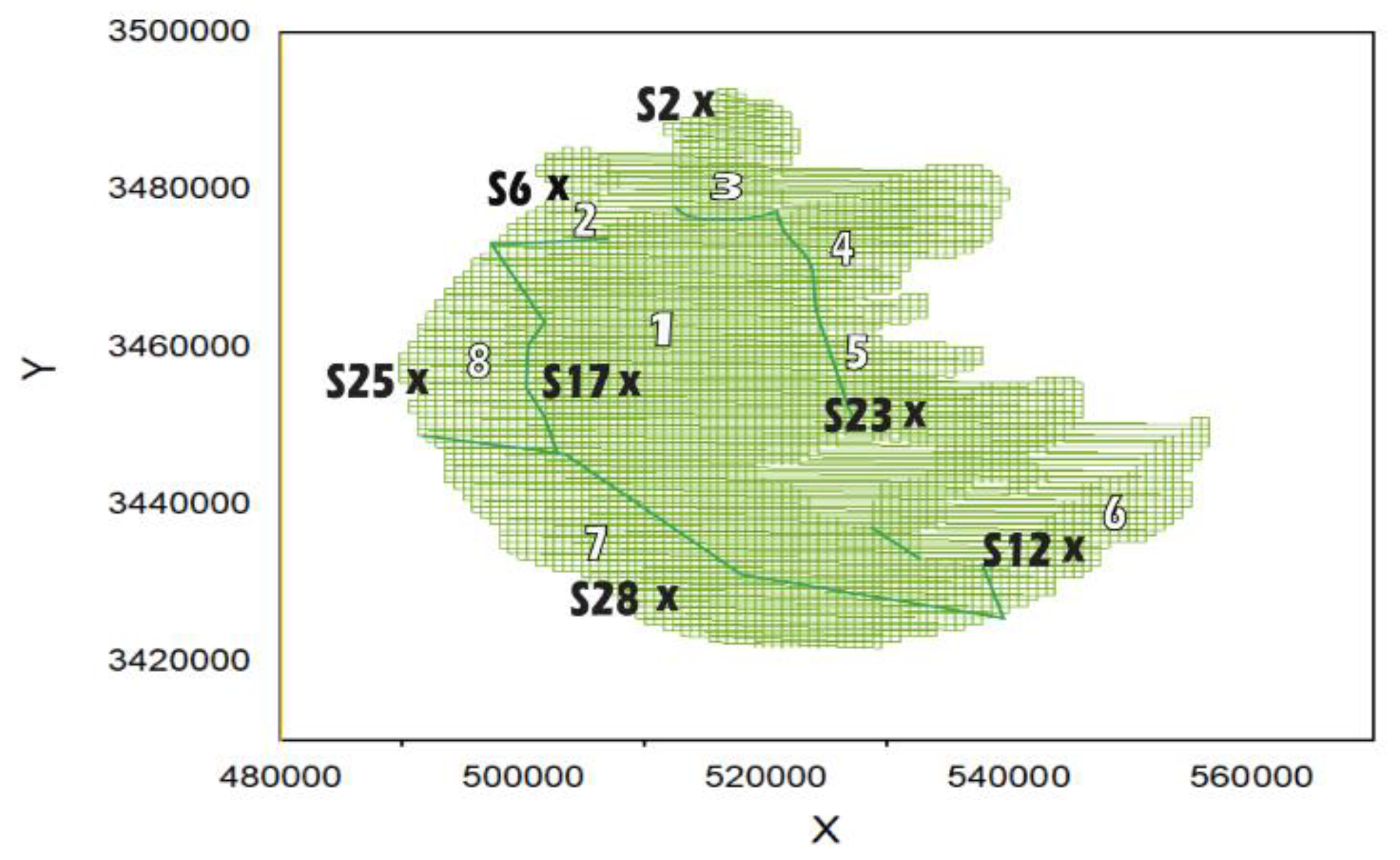
2.1. The Research Area

Lake Taihu, with its complex shoreline geometries, is connected to 172 rivers or channels and is the third-largest shallow freshwater lake in China [19]. It is located between 119°08′–122°55′ E and 30°05′–32°08′ N, having a catchment area of 36,500 km² with a surface area of 2338 km² [3]. The mean (maximum) depth of the lake is 1.9 m (2.6 m), corresponding to an elevation of 3.0 m [3]. The lake bottom features a flat terrain with a mean geographic gradient of 0°0′19.66″.

A shallow-water area with an average depth of < 1.5 m is sited in the eastern part and accounts for 19.3% of the total surface area. The deepest areas (>2.5 m), occupy nearly 8.4% of the total lake area, and are in the north and west. According to field observations, thermal stratification is not explicitly evident, even though it exists on the lake. Its duration is typically less than one day, as it is easily mixed by wind force [3,31]. Moreover, the temperature difference from the surface to the bottom mostly ranges from 0–1 °C and other cases of 1–4 °C per field monitoring data available from December 2007 to November [32]. The leading wind direction on the lake is southeast in the summer and northwest in the winter at an average wind speed of 3.5–5 m/s [3]. For easy monitoring and management of Lake Taihu, it has been divided into eight subareas: Zhushan Bay, Meiliang Bay, Gonghu Bay, Northwest Zone, Southwest Zone, Central Zone, East Epigeal Zone, and Dongtaihu Bay (Figure 1).

2.2. The Role of the Environmental Fluid Dynamics Code

A three-dimensional hydrodynamic model originally developed by John Hamrick called the Environmental Fluid Dynamic Code (EFDC) was utilized to simulate the seasonal variation of sediment flux on Lake Taihu [33]. The model is one of the most widely applied advanced modeling frameworks for simulating hydrodynamics, water quality, eutrophication, and dynamic changes and interactions in sediment transportation in lakes, rivers, and estuaries [18].

It has 22 state variables in the water column and is coupled with 27 state variable sediment diagenesis models. The sediment diagenesis model is based on a recording of the model developed by DiToro and Fitzpatrick [9]. The sediment diagenesis model receives particulate organic matter (POM), in this case, specifically particulate organic nitrogen (PON), which has been deposited from the water column.

EFDC then simulates the diagenesis, and the resulting fluxes of nitrate (NO₃) and ammonium (NH₄) escape back into the water column. The water quality model is coupled with sediment diagenesis. This coupling of the models not only enhances predictively, but gives room to simulate long term variations [24]. Countless studies have used this tool, and its demonstration shows its convenience, faster calculation times, accuracy, robustness, and reproducibility [34]. Nevertheless, this approach has not been applied to Lake Taihu.

2.3. Principles of Diagenesis Fluxes

The principle of mass conservation governs sediment diagenesis models like water quality models. The diagenesis expression used, which is the kinetic equation for particulate organic nitrogen (PON) is based on the mass balance equation:

Net PON change = − decay of PON − burial + depositional flux

(1)

The depositional fluxes settle directly at the lower part of the lake called the lower layer or L2 in EFDC. Diagenesis occurs only in the lower layer. The upper layer, L1(aerobic) is considered as not significant because of its small thickness: L1; $H_{1 }$= 0.1 cm, while L2; $H_{2 }$= 10 cm.

$$H_{2 }\frac{d{G}_{PON{,}_{i }}}{dt}=-k_{PON{,}_{i }}{\theta }_{PON{,}_{i }}^{\left(T-20\right)} G_{PON{,}_{i }}{H}_{2 }-{\mathsf{\omega }}_{ } G_{PON{,}_{i }}+J_{PON{,}_{i } }$$

(2)

where $G_{PON{,}_{i }}$ is the PON concentration in ith G class (Layer 2(g/m³) in the anaerobic layer; $k_{PON{,}_{i }}$ is the decay rate of the ith G class PON at 20 °C in Layer 2(day⁻¹); ${\theta }_{PON{,}_{i }}$ is the constant temperature adjustment for $k_{PON{,}_i}$; T is the sediment temperature (°C); and $\mathsf{\omega }$ is the burial rate (m/day). $J_{PON{,}_{i }}$ is the depositional fluxes that serve as a source term to drive the diagenesis process [32].

2.4. Constructing the Sediment Diagenesis of Nitrate (NO₃), Ammonium–Nitrogen Flux Model

Twelve (12) parameters were selected for the sediment diagenesis model chosen through a detailed investigation of the literature, creating an input file with the Latin hypercube sampling method (LHS) (

Table 1. Environmental Fluid Dynamics Code (EFDC) sediment diagenesis model related variables and fluxes.

No	Parameter	Meaning	Unit	Range
1	Dp	Particle mixing apparent diffusion coefficient	m2/d	<0.001–0.5
2	θDpThDp	Constant for temperature adjustment for Dp	-	1.07–1.117
3	Hsed	Diagenesis sediment thickness	m	0.10–0.20
4	W2	Sediment burial rate	cm/yr	0.02–1.0
5	θNH4/ThNH4	Temperature coefficient for nitrification	-	1.076–1.127
6	KN03,1	Reaction velocity for denitrification in the aerobic layer	m/d	0.05–0.10
7	θNO3/ThNO3	Temperature coefficient for denitrification	-	1.056–1.20
8	KPON1	Decay rate of PON at 20 °C for G1 class	1/d	0.019–0.066
9	ThKN1	Constant for temperature adjustment for KPON1	-	1.052–1.166
10	ThKN2	Constant for temperature adjustment for KPON2	-	1.052–1.166
11	θKM,NH4	Temperature coefficient for nitrification half-saturation constant	-	1.125
12	KPON2	Decay rate of PON at 20degC for G2 class	1/d	0.0012–0.0088

). The LHS approach generates a sequence for every possible combination of the independent input parameters. It works by taking the range of each independent parameter, dividing the range by the selected realizations, rearranging the values into a random distribution, and then combining the distributions for each independent parameter [35].

A set of 200 parameter combinations was produced by the LHS random sampling and incorporated into the EFDC water quality model by [1,35]. The EFDC nitrate (NO₃) and NH₄ flux Taihu model was set up in a horizontal Cartesian coordinate system divided into 4,465,750 m x 750 m square meshes with a uniform grid, as shown in Figure 1. The grid is vertically divided into three layers using σ coordinates. The slope of the model lake bottom was less than 0.33, preventing the pressure caused by the σ coordinates.

The force gradient error serves as input as the boundary condition of the model by the atmosphere, wind speed and direction, lake flow, water quality, and sediment. The atmospheric conditions and wind farms were based on the Nanjing Geography and Lake Research Institute of the Chinese Academy of Sciences, and data from the National Field Observation and Research Station of the Taihu Lake Ecosystem.

The initial simulation date was 20 June, and assumed as initial. The water level was horizontal and set to the average of the first day of the simulation period. The initial flow rate was set to 0 m/s. Model calculation time was 365 days, and the time step was one (1) minute. The model was run 200 times to ensure standard calibration, accuracy, and reproducibility.

2.5. Data Recording Stations

Seven (7) S data recording stations from the National Field Observation and Research Station on Taihu Lake across all eight (8) zones of Figure 1 were used for calibration, namely; (S2) Small Wanli, (S6) Zhu Lake, (S12) East Taihu Lake, (S17) Platform Mountains, (S23) Xu Lake, (S25) V. East, and (S28) Xiaomei Mouth. Since EFDC sediment diagenesis model allows coupling with the water quality model, the available measured water quality values of total nitrogen (TN) for the seven (7) S stations were used. TN was considered because the EFDC sediment diagenesis model uses nitrogen related parameters.

3. Results

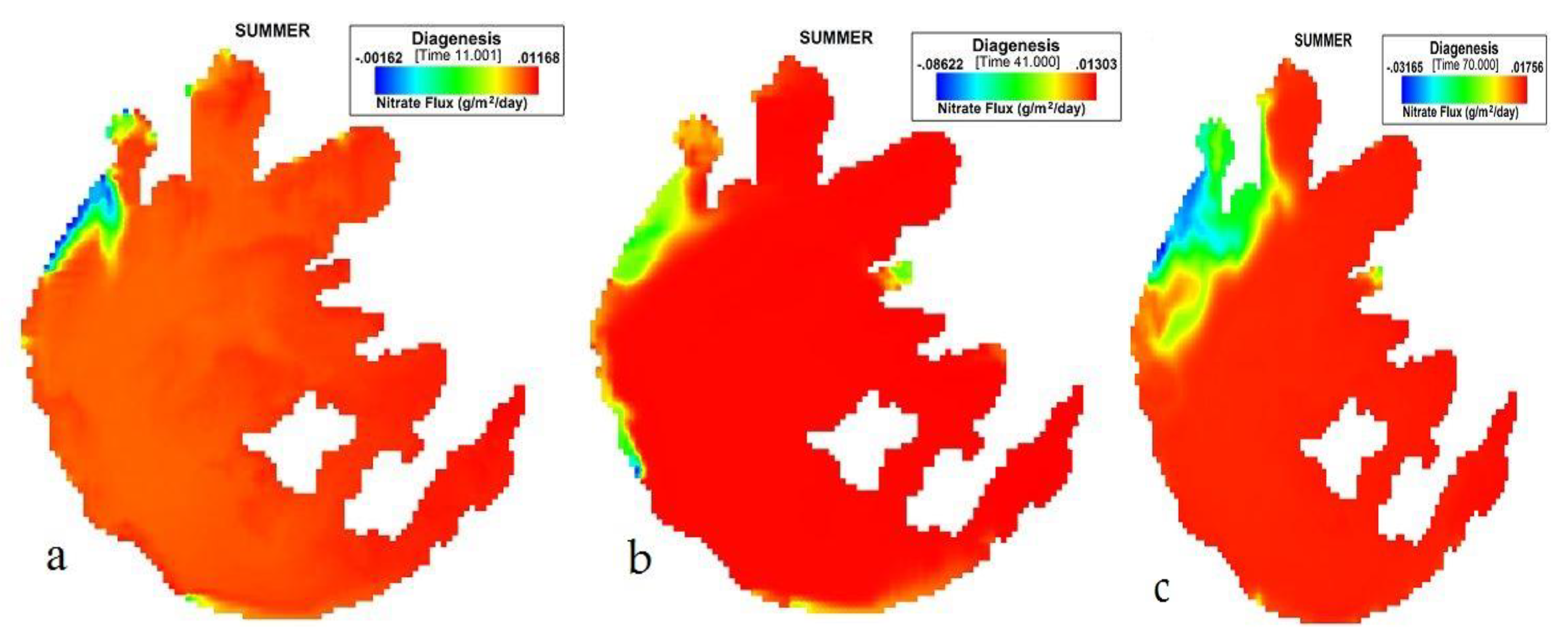
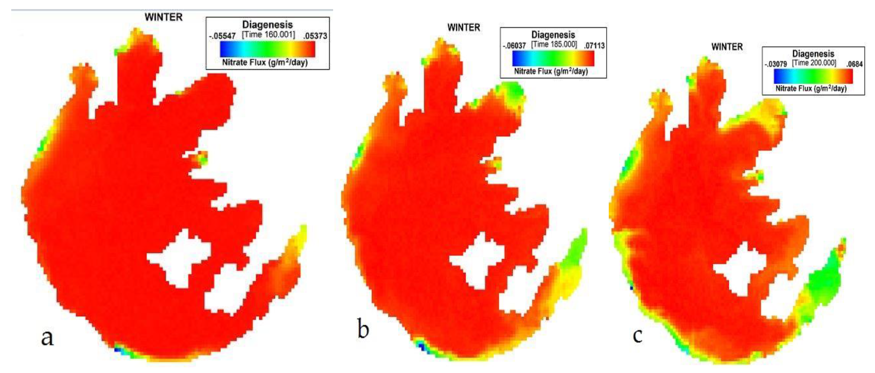
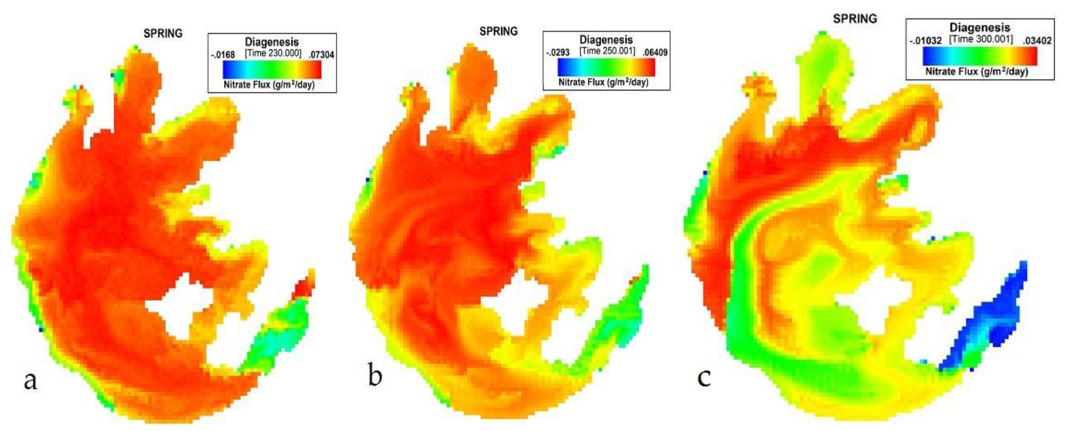
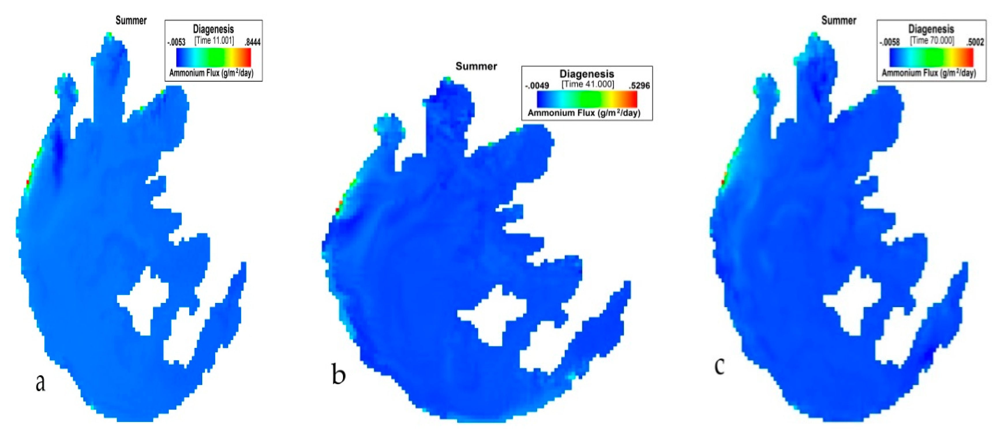
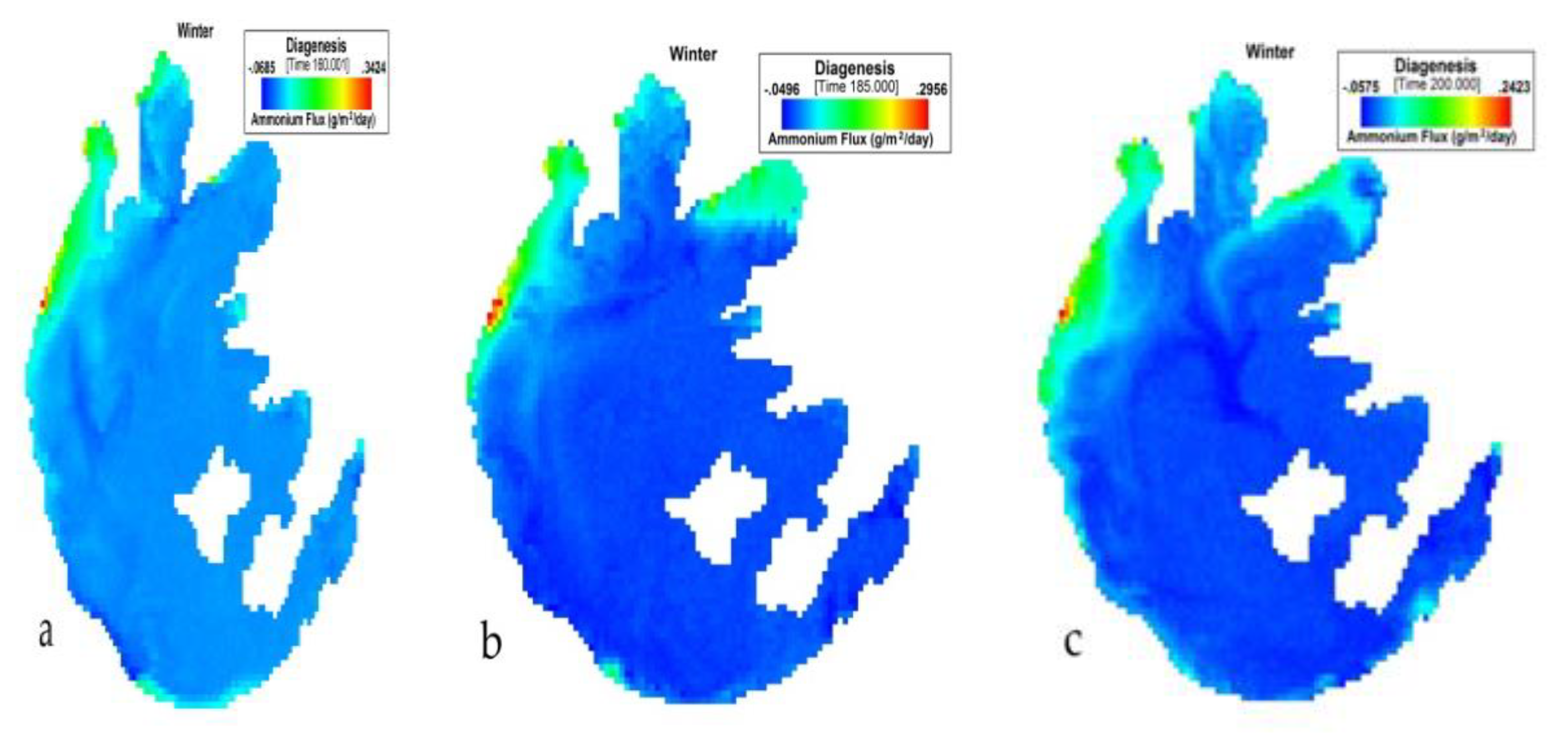
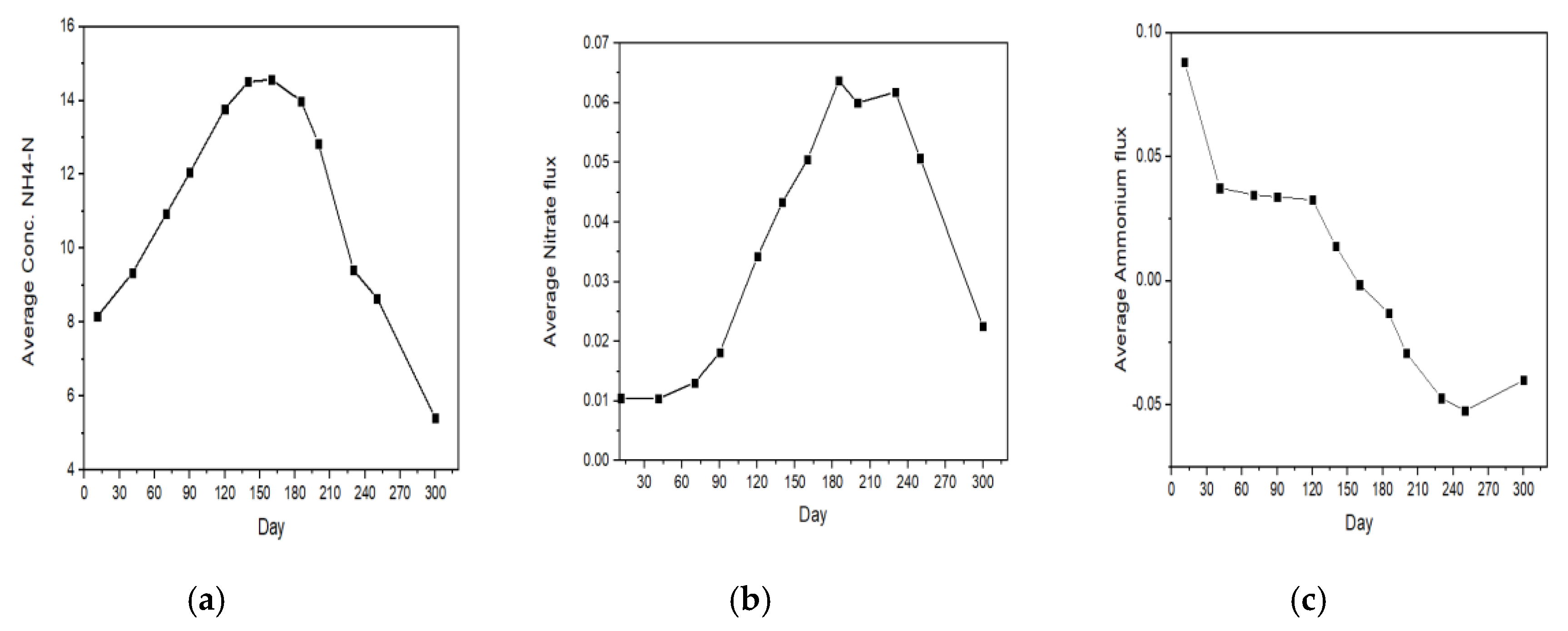
3.1. Seasonal Variation of Nitrate (NO₃) Flux Analysis

The outcome of the simulation presented 17,856 simulated data points each day for 365 days because of the number of nodes. Due to the large datasets, some days were selected based on the critical times present in each month of the year. The eleventh day was chosen, which was the last day in June, based on the initial time of the simulation because the variation of the fluxes would have started showing after 10 days of waiting.

The 41st day was almost at the end of July, and the 70th day was at the end of August. These selected days would have had ample time to manifest the variations of the fluxes. The same understanding was applied to the 90th, 120th, and 140th days present in September, October, and November, respectively. In addition, the 160th, 185th, and 200th days were calculated from December, January, and February, respectively.

Finally, the 230th, 250th, and the 300th days were also selected based on the initial date of simulation from March, April, and May, respectively. A direct comparison was made at a seasonal timescale. Winter was defined as December–January–February (DJF), spring as March–April–May (MAM), summer as June–July–August, (JJA), and autumn as September–October–November, (SON).

Figure 2 presents the simulation of NO₃ flux variation during JJA on Taihu. Nitrate flux variation during summer began from the northwest zone of Taihu and a little at the boundary of Zhushan Bay with the lowest influx of −0.06622, an average of 0.011333 (g/m²/day),

Table 2. Shows the seasonal, ranges, and average concentration of NH₄–N, sediment fluxes of NO₃, and NH₄ at Lake Taihu.

Time (Days)	Range (g/m2/Day)	Range (g/m3)	Range (g/m2/Day)	Average (g/m2/Day)	Range (g/m3)	Average (g/m2/Day)
	NO3 Flux	Conc. NH4-N	NH4 Flux	NO3 Flux	Conc.NH4-N	NH4 Flux
11th	−0.0162–0.01168	7.469671–18.81496	−0.005–0.844	0.0105	8.158883	0.08814
41st	−0.06622–0.01303	5.262655–19.0483	−0.0049–0.5296	0.0104	9.332679	0.03746
70th	−0.03165–0.01756	9.191248–17.47765	−0.0058–0.5002	0.0131	10.93654	0.0347
90th	−0.01081–0.0211	9.594671–19.50419	0.0187–0.4464	0.018149	12.0526	0.03385
120th	−0.04543–0.04031	4.2638–22.48205	−0.033–0.4914	0.0342	13.78247	0.03268
140th	−0.03398–0.04587	6.443372–22.31578	−0.0372–0.0746	0.0433	14.50533	0.01396
160th	−0.05547–0.5373	4.224813–22.38613	−0.0685–0.3424	0.0505	14.57058	−0.00146
185th	−0.06037–0.07113	4.278185–19.12033	−0.0496–0.2956	0.0637	13.99708	−0.01295
200th	−0.03079–0.0684	5.261141–18.6685	−0.0575–0.2429	0.0600	12.8486274	−0.02501
230th	−0.0163–0.07304	3.025818–13.67934	−0.0871–0.2172	0.0618	9.413582	−0.04715
250th	−0.0293–0.0649	5.151477–11.53736	−0.0838–0.1551	0.0507	8.65485	−0.05229
300th	−0.0102–0.03402	2.744903–9.846215	−0.0515–0.081	0.0223	5.405481	−0.03999

. The highest flux value during JJA was 0.01756 as shown on the 70th day. There was a gradual rise in the sediment flux of nitrate. Based on the values during this period, the rate of nitrate flux escaping into the water column was very low.

Figure 3 presents the simulation of NO₃ flux variation during SON in Taihu. Its sediment flux ranges from 0.018149 to 0.0433 (g/m²/day). The lowest influx was −0.04543 (g/m²/day), an average of 0.031883 (g/m²/day).

Figure 4 presents the simulation of NO₃ flux variation during winter on Taihu. During DJF, the nitrate (NO₃) flux variation extended gradually from all seven boundaries toward the central zone with a range of −0.03079 to 0.0684 (g/m²/day), but with the highest average value of 0.0637 (g/m²/day). The lowest influx was −0.06037 (g/m²/day) with an average of 0.058067 (g/m²/day).

Finally, in spring (MAM), from Figure 5, the lowest influx was −0.0163, with an average of 0.044933. The nitrate flux values started declining from the 231st day to the last day. The average sediment flux values dropped from 0.0618 to 0.0223 (g/m²/day).

3.2. Seasonal Variation of Concentration Ammonium–Nitrogen (Conc. NH₄–N) Analysis

The results showed Layer 1 and 2 (L1 and L2, respectively). Due to the negligible nature of L1, the results shown in Table 2 are from L2m which is where diagenesis occurs. Diagenesis of the concentration of NH₄–N in the sediment–water column increased from 2.744903 to 22.38613 (g/m³) (see Table 2). The highest efflux was experienced during winter 22.38613 (g/m³), which also had the highest average concentration. Compared to the nitrate (NO₃) flux, the lowest concentration of NH₄–N was experienced in spring, while it was nitrate during summer.

Figure 6 presents the simulation of NH₄ flux variation during summer in Taihu. During JJA, the NH₄ flux variation had the lowest value of −0.0058 (g/m²/day) and an average of 0.053433 (g/m²/day). The highest value for this period was 0.844 (g/m²/day).

Figure 7 presents the simulation of NH₄ flux variation during autumn in Taihu. During SON, the NH₄ flux variation also had the lowest value of −0.0372 (g/m²/day) and an average of 0.02683 (g/m²/day). The highest value for this period was 0.03385 (g/m²/day).

Figure 8 presents the simulation of NH₄ flux variation during winter in Taihu. During DJF, the NH₄ flux variation had the lowest value of −0.0685 (g/m²/day) and an average of −0.01314 (g/m²/day). The highest value for this period was 0.3424 (g/m²/day).

Figure 9 presents the simulation of NH₄ flux variation during spring in Taihu. During MAM, the NH₄ flux variation had the lowest value of −0.0871 (g/m²/day) and an average of −0.046476667 (g/m²/day). The highest value for this period was 0.2172 (g/m²/day).

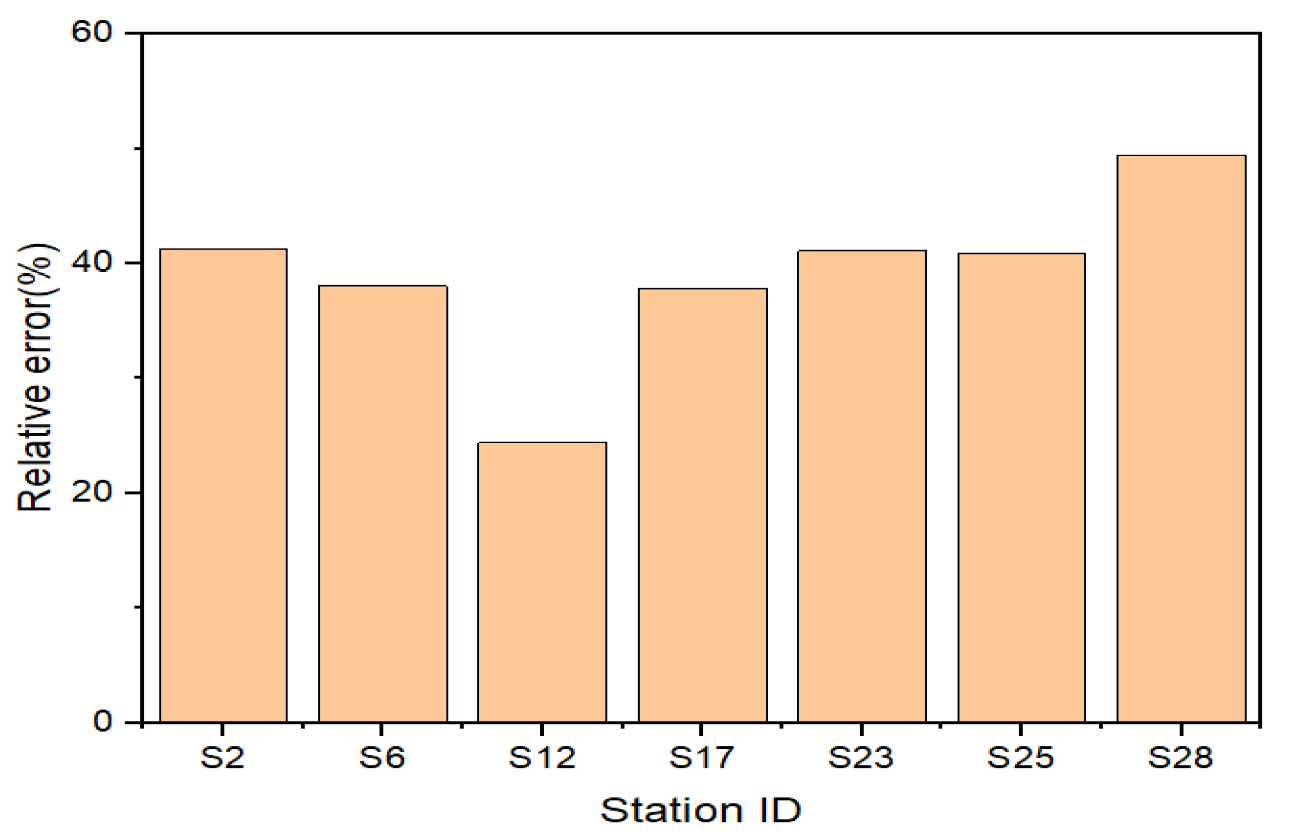
3.3. Calibration of the Lake Taihu Sediment Diagenesis Model with the Water Quality Model

The measured data averaged from 1.082 to 3.593 (mg/l), while the model data averaged from 0.907 to 3.158(mg/l) at Taihu. The relative error ranged from 24.377% to 49.417%.

4. Discussion

The implications of the summary of results in Figure 10 explains that in summer, ammonium (NH₄) fluxed out of the sediment with very little oxidation to nitrate (NO₃). As a result, ammonium (NH₄) accumulated in the water column. This is consistent with anoxic conditions. The flux of nitrate at that time was not negative (assuming that the positive flux means out of the sediment). Nitrate (NO₃) was expected to flux into the sediment under anoxic conditions. Perhaps the concentration of nitrate (NO₃) was very low in the water column at that time.

In autumn and winter, the sediment is most likely progressively oxidized. As a result, more of the sediment ammonium oxidized to nitrate. The flux of ammonium decreased, while the flux of nitrate (NO₃) increased. The concentration of ammonium continued to increase until around day 150 because the flux of ammonium was still positive.

After day 150, the sediment became a sink for ammonium, implying that the oxidation of ammonium occurred in the sediment much faster than in the water column. The negative flux caused the ammonium concentrations to decrease. The continued oxidation of ammonium, however, continued to produce nitrate (NO₃). The results were consistent. This would allow algal blooms to continue to thrive in the lake, creating a threat to water quality sustainability.

With the onset of low-oxygen conditions in spring, denitrification intensified, which consumed nitrate (NO₃) by converting it predominantly to nitrogen gas. Part of it may be converted to ammonium via dissimilatory nitrate reduction to ammonium (DNRA).

Due to similar conditions of eutrophic Lake Taihu, Lake Okeechobee, and Chesapeake Bay, the pattern of this model was compared with Conc. NH₄–N of Lake Okeechobee and the nitrate flux of Chesapeake Bay. From Lake Okeechobee, in July 1999, there was an increase in Conc. NH₄–N in the sediment–water column from 0.03 in the water column to 2 (g/m³) in the sediment pore water. The lake’s pore water concentration NH₄–N also continued to increase with depths below the sediment–water interface [18]. Additionally, at Chesapeake Bay, from the measured data, one half of the nitrate formed by nitrification of diagenetically produced ammonia escaped as nitrate flux to the overlying water.

Additionally, almost all nitrate produced by sediment nitrification denitrified to nitrogen gas [9]. There was an alignment of the pattern of the results and affirmed similar behavior and observations. The range of values of this model fell within the nitrate (NO₃) flux of Chesapeake Bay 0.05–0.10 (g/m²/day) [9].

Furthermore, Elorn and Aulne, two small eutrophic estuaries in France, explained a spatio-temporal variability of the sediment organic matter recycling distribution of nitrate (NO_x) and NH₄⁺. The two estuaries experienced a large suboxic and anoxic mineralization at the sediments, causing rapid removal of very high bottom water concentrations of nitrate (NO_x) and the large NH₄⁺ increase at depth at all stations. Nitrate (NO_x) concentrations decreased between winter and spring [36]. Hence, denitrification also occurred in these estuaries during spring.

On the archipelago of the Gulf of Finland, Baltic Sea resuspension promoted nitrification, with an indication seen in increased NOx fluxes at both stations at 7 m and 20 m (by 30% and 27% respectively) and a lowered NH₄ flux (by 48%) at the 7 m station for the month of May and August [37]. In freshwater systems and other coastal bodies, NH₄⁺ is recognized by most algal species, particularly Cyanophyta, as the preferred nitrogen source for growth [38,39]. While bloom severity within each subdivision on western Lake Erie is temporally and spatially unique, it increased over the study period of July to October 2002–2016 [40].

During autumn in Xiangxi Bay of the Three Gorges Reservoir, China, there is increasing nutrient loading from anthropogenic sources, which adequately decreases the ecological diversity [38].

However, seasonal bloom distribution for the period of 2002–2011 on Lake Winnipeg was consistent with light limitation in the south basin and lake circulation transporting bloom material toward the north-east shore, which could be the result of low oxygen at the sediment. Inter-annual variability in average bloom severity was related to both total phosphorus (TP) loadings and summer lake surface temperatures [29].

The evaluation results on Lake Chaohu revealed that effective HABs control in the lake depended on reducing P loading. Both internal and external P loading contributed significantly to HABs in the lake. August, May, and July were the hot moments for external P reduction. The Nanfei and Hangbu Rivers were hot spots for external P reduction [33]. Algae carbon is said to greatly consume oxygen at the benthic region, preventing denitrification from occurring. While nitrate denitrifies during spring and summer into nitrogen gas, phosphorus is not removed by this biochemical reaction. Future work would explore these areas. To ensure accuracy and quality of the simulated values, the results were calibrated. The total impression of the calibration (Figure 11) is that the model fluxes were in reasonable agreement [23,24]. The model was also found to be suitable because the average relative error for the TN was 38.137%.

5. Conclusions

Sediment flux has a significant contribution to lake management since it is established that it becomes a source for resuspension. During summer, the accumulation of ammonium (NH₄) in the water column due to oxidation of nitrate (NO₃) creates an environment for algal bloom. In autumn and winter, the elevated nitrate (NO₃) and the concentration of ammonium levels increased the rate of algae producing toxins in the lake, which would cause immense contamination. As a result, an unhealthy aquatic environment is created for the organisms and reduces the suitability of water for human consumption.

Coupled with TN water quality measured data calibration at the lake, the relative error was below forty percent (40%), which makes the model suitable. The seasonal variation of sediment flux at Taihu provides the essence that creates awareness for more wholesome models on lakes for the sustainability of its water quality. Future studies should aim to simulate phosphate flux and provide measurements of the fluxes on the lake.

References

1. Jiang, L.; Li, Y.; Zhao, X.; Tillotson, M.R.; Wang, W.; Zhang, S.; Sarpong, L.; Asmaa, Q.; Pan, B. Parameter uncertainty and sensitivity analysis of water quality model in Lake Taihu, China. Ecol. Model. 2018, 375, 1–12. [Google Scholar] [CrossRef]
2. Emerson, S.; Hedges, J. Sediment diagenesis and benthic flux. Treatise Geochem. 2003, 6, 293–319. [Google Scholar]
3. Hu, W.; Chen, Y. Sediment resuspension in the lake Taihu, China. Chin. Sci. Bull. 2014, 41, 420–425. [Google Scholar] [CrossRef]
4. Chunhua, H.; Weiping, H.; Fabing, Z.; Zhixin, H.; Xianghua, L.; Yonggen, C. Sediment resuspension in the lake Taihu, China. Chin. Sci. Bull. 2006, 51, 731–737. [Google Scholar]
5. Dzialowski, A.R.; Wang, S.; Lin, N.-C.; Beury, J.H.; Huggins, G.D. Effects of sediment resuspension on nutrient concentrations and algal biomass in reservoirs of the central plains. Lake Reservioirs Manag. 2008, 24, 313–320. [Google Scholar] [CrossRef] [Green Version]
6. Sobek, S.; Zurbru, R.; Ostrovsky, I. The burial efficiency of organic carbon in the sediments of lake kinneret. Aquat. Sci. 2011, 73, 355–364. [Google Scholar] [CrossRef] [Green Version]
7. Hansen, P.S.; Phlips, E.J.; Aldridge, F.J. The effects of sediment resuspension on phosphorus available for algal growth in a shallow subtropical lake, lake okeechobee. Lake Reservioirs Manag. 1997, 13, 154–159. [Google Scholar] [CrossRef] [Green Version]
8. Kaiser, D.; Kowalski, N.; Böttcher, M.E.; Yan, B.; Unger, D. Benthic nutrient fluxes from mangrove sediments of an anthropogenically impacted estuary in southern china. Mar. Sci. Eng. 2015, 3, 466–491. [Google Scholar] [CrossRef] [Green Version]
9. Di Toro, D.M.; Fitzpatrick, J.J. Chesapeake Bay Sediment Flux Model; U.S. Army Corps of Engineers, Waterways Experiment Station: Vicksburg, MS, USA, 1993.
10. McCulloch, J.; Gudimov, A.; Arhonditisis, G.; Chesnyuk, A.; Dittrich, M. Dynamics of p-binding forms in sediments of a mesotrophic hard-water lake: Insights from non-steady state reactive-transport modeling, sensitivity and identifiability analysis. Chem. Geol. 2013, 354, 216–232. [Google Scholar] [CrossRef]
11. Li, L.; Ni, J.; Chang, F.; Yue, Y.; Frolova, N.; Magritsky, D.; Borthwick, A.G.L.; Ciais, P.; Wang, Y.; Zheng, C.; et al. Global trends in water and sediment fluxes of the world’ s large rivers. Sci. Bull. 2019, 65, 62–69. [Google Scholar] [CrossRef] [Green Version]
12. Policelli, F.; Hubbard, A.; Jung, H.C.; Zaitchik, B. A predictive model for lake chad total surface water area using remotely sensed and modeled hydrological and meteorological parameters and multivariate regression analysis. J. Hydrol. 2018, 568, 1071–1080. [Google Scholar] [CrossRef]
13. Duan, L.; Song, J.; Liang, X.; Yin, M.; Yuan, H.; Li, X. Dynamics and diagenesis of trace metals in sediments of the changjiang estuary. Sci. Total Environ. 2019, 675, 247–259. [Google Scholar] [CrossRef] [PubMed]
14. Binding, C.E.; Greenberg, T.A.; McCullough, G.; Watson, S.B.; Page, E. An analysis of satellite-derived chlorophyll and algal bloom indices on lake winnipeg. J. Great Lakes Res. 2018, 44, 436–446. [Google Scholar] [CrossRef]
15. Watson, S.B.; Miller, C.; Arhonditsis, G.; Boyer, G.L.; Carmichael, W.; Charlton, M.N.; Confesor, R.; Depew, D.C.; Hook, T.O.; Ludsin, S.A.; et al. The re-eutrophication of lake erie: Harmful algae blooms and hypoxia. Harmful Algae 2016, 56, 44–66. [Google Scholar] [CrossRef] [PubMed]
16. Qin, B.; Xu, P.; Wu, Q.; Luo, L.; Zhang, Y. Environmental issues of lake taihu, china. Hydrobiologia 2007, 58, 3–14. [Google Scholar]
17. Gao, L.; Zhou, J.M.; Yang, H.; Chen, J. Phosphorus fractions in sediment profiles and their potential contributions to eutrophication in dianchi lake. Environ. Geol. 2005, 48, 835–844. [Google Scholar] [CrossRef]
18. Huang, J.; Zhang, Y.; Huang, Q.; Gao, J. When and where to reduce nutrient for controlling harmful algal blooms in large eutrophic lake chaohu, china? Ecol. Indic. 2018, 89, 808–817. [Google Scholar] [CrossRef]
19. Kim, D.; Zhang, W.; Watson, S.; Arhonditsis, G. A commentary on themodelling of the causal linkages among nutrient loading, harmful algal blooms, and hypoxia patterns in lake erie. J. Great Lakes Res. 2014, 40, 117–129. [Google Scholar] [CrossRef]
20. Yadav, N.; Kour, D.; Yadav, A.N. Microbiomes of freshwater lake ecosystems. J. Microbiol. Exp. 2018, 6, 245–248. [Google Scholar] [CrossRef] [Green Version]
21. Nwankwegu, A.S.; Li, Y.; Huang, Y.; Wiei, J.; Norgbey, E.; Sarpong, L.; Lai, Q.; Wang, K. Harmful algal blooms under changing climate and constantly increasing anthropogenic actions: The review of management implications. 3 Biotech 2019, 9, 449. [Google Scholar] [CrossRef]
22. Pena, M.A.; Katsev, S.; Oguz, T.; Gilbert, D. Modeling dissolved oxygen dynamics and hypoxia. Biogeosciences 2010, 7, 933–957. [Google Scholar] [CrossRef] [Green Version]
23. Katsev, S.; Dittrich, M. Modeling of decadal scale phosphorus retention in lake sediment under varying redox conditions. Ecol. Modell. 2013, 251, 246–259. [Google Scholar] [CrossRef]
24. Tang, G.; Zhu, Y.; Wu, G.; Li, J.; Li, Z.-L. Modelling and analysis of hydrodynamics and water quality for rivers in the northern cold region of china. Int. J. Environ. Res. Public Health 2016, 13, 408. [Google Scholar] [CrossRef] [PubMed] [Green Version]
25. Qin, B.; Xu, P.; Wu, Q.; Luo, L.; Zhang, E.Y. Environmental issues of lake Taihu, China. In Eutrophication of Shallow Lakes with Special Reference to Lake Taihu, China; Springer: Dordrecht, The Netherlands, 2007. [Google Scholar]
26. Deng, B.; Liu, S.; Xiao, W.; Wang, W.; Jin, J.; Lee, X. Evaluation of the clm4 lake model at a large and shallow freshwater lake. J. Hydrometeorol. 2013, 14, 636–649. [Google Scholar] [CrossRef] [Green Version]
27. Janssen, A.B.G.; Jager, V.C.L.D.; Janse, J.H.; Kong, X.; Liu, S.; Ye, Q.; Mooij, W.M. Spatial identification of critical nutrient loads of large shallow lakes: Implications for lake Taihu (China). Water Res. 2017, 119, 276–287. [Google Scholar] [CrossRef] [PubMed]
28. Huo, S.; He, Z.; Ma, C.; Zhang, H.; Xi, B.; Zhang, J.; Li, X.; Wu, F.; Liu, H. Spatio-temporal impacts of meteorological and geographic factors on the availability of nitrogen and phosphorus to algae in chinese lakes. J. Hydrol. 2019, 572, 380–387. [Google Scholar] [CrossRef]
29. Liang, S.; Wu, H.; Li, H.; Wu, Y. Assessment of the spatial and temporal water eutrophication for lake baiyangdian based on integrated fuzzy method. J. Environ. Prot. 2013, 4, 120–125. [Google Scholar] [CrossRef] [Green Version]
30. Wu, T.; Qin, B.; Brookes, J.D.; Yan, W.; Ji, X.; Feng, J. Spatial distribution of sediment nitrogen and phosphorus in lake taihu from a hydrodynamics-induced transport perspective. Sci. Total Environ. 2019, 650, 1554–1565. [Google Scholar] [CrossRef]
31. Kämpf, J. Wind-driven overturning, mixing and upwelling in shallow water: A nonhydrostatic modeling study. J. Mar. Sci. Eng. 2017, 5, 47. [Google Scholar] [CrossRef] [Green Version]
32. Zhang, Y.; Qin, B.-Q.; Zhu, G.; Gao, G. Effect of sediment resuspension on underwater light field in shallow lakes in the middle and lower reaches of the yangtze river: A case study in Longgan lake and Taihu lake. Sci. China Ser. D 2014, 49, 114–125. [Google Scholar] [CrossRef]
33. Tech, T. The environmental fluid dynamics code theory and computation: Sediment and contaminant transport and fate. Tetra. Tech. Inc. 2008, 2, 635–639. [Google Scholar]
34. Chen, Y.; Zou, R.; Su, H.; Bai, S.; Faizullabhoy, M.; Wu, Y. Development of an integrated water quality and macroalgae simulation model for tidal marsh eutrophication control decision support. Water 2017, 9, 277. [Google Scholar] [CrossRef] [Green Version]
35. Taylor, P.; Li, Y.; Tang, C.; Zhu, J.; Pan, B.; Anim, D.O.; Ji, Y. Parametric uncertainty and sensitivity analysis of hydrodynamic processes for a large shallow freshwater lake parametric uncertainty and sensitivity analysis of hydrodynamic processes for a large shallow freshwater lake. Hydrol. Sci. J. 2015, 60, 1078–1095. [Google Scholar]
36. Khalil1, K.; Raimonet, M.; Laverman, A.M.; Yan, C.; Andrieux-Loyer, F.; Viollier, E.; Deflandre, B.; Ragueneau, O.; Rabouille, C. Spatial and temporal variability of sediment organic matter recycling in two temperate eutrophicated estuaries. Aquat. Geochem. 2013, 19, 517–542. [Google Scholar] [CrossRef] [Green Version]
37. Niemistö, J.; Kononets, M.; Ekeroth, N.; Tallberg, P.; Tengberg, A.; Hall, P.O.J. Benthic fl uxes of oxygen and inorganic nutrients in the archipelago of gulf of finland, baltic sea—Effects of sediment resuspension measured in situ. J. Sea Res. 2018, 135, 95–106. [Google Scholar] [CrossRef] [Green Version]
38. Nwankwegu, A.S.; Li, Y.; Huang, Y.; Wei, J.; Norgbey, E.; Lai, Q.; Sarpong, L.; Wang, K.; Ji, D.; Yang, Y.; et al. Nutrient addition bioassay and phytoplankton community structure monitored during autumn in xiangxi bay of three gorges reservoir, china. Chemosphere 2020, 247, 125960. [Google Scholar] [CrossRef] [PubMed]
39. Paerl, W.H.; Fulton, S.R.; Moisander, P.H.; Dyble, J. Harmful freshwater algal blloms, with an empahsis on cyanobacteria. Sci. World 2001, 1, 76–113. [Google Scholar] [CrossRef] [PubMed]
40. Manning, N.F.; Wang, Y.; Long, C.M.; Bertani, I.; Sayers, M.J.; Bosse, K.R.; Shuchman, R.A.; Scavia, D. Extending the forecast model: Predicting western lake erie harmful algal blooms at multiple spatial scales. J. Great Lakes Res. 2019, 45, 587–595. [Google Scholar] [CrossRef]
Figure 1. Eutrophic Lake Taihu in its grid form. Zones: (1) Central Zone, (2) Zhushan Bay, (3) Meiliang Bay, (4) Gonghu Bay, (5) East Epigeal Zone, (6) DongTaihu Bay, (7) Southwest Zone, (8) Northwest Zone, and data recording stations (S).
Ijerph 17 04158 g001
Figure 2. (a) 11th, (b) 41st, (c) 70th day simulation of NO3 flux variation during summer at Taihu.
Ijerph 17 04158 g002
Figure 3. (a) 90th, (b) 120th, (c) 140th day simulation of NO3 flux variation during autumn at Taihu.
Ijerph 17 04158 g003
Figure 4. (a) 160th, (b) 185th, (c) 200th day simulation of NO3 flux variation during winter at Taihu.
Ijerph 17 04158 g004
Figure 5. (a) 230th, (b) 250th, (c) 300th day simulation of NO3 flux variation during spring at Taihu.
Ijerph 17 04158 g005
Figure 6. (a) 11th, (b) 41st, (c) 70th day simulation of NH4 flux variation during summer at Taihu.
Ijerph 17 04158 g006
Figure 7. (a) 90th, (b) 120th, (c) 140th day simulation of NH4 flux variation during autumn at Taihu.
Ijerph 17 04158 g007
Figure 8. (a) 160th, (b) 185th, (c) 200th day simulation of NH4 flux variation during winter at Taihu.
Ijerph 17 04158 g008
Figure 9. (a) 230th, (b) 250th, (c) 300th day simulation of NH4 flux variation during spring at Taihu.
Ijerph 17 04158 g009
Figure 10. Seasonal variation of (a) average Conc NH4–N, (b) average nitrate (NO3); and (c) average ammonium (NH4) fluxes at Taihu, China.
Ijerph 17 04158 g010
Figure 11. Average relative error for the water quality parameter total nitrogen (TN) at Taihu, China.
Ijerph 17 04158 g011