Article

Can Green Walls Reduce Outdoor Ambient Particulate Matter, Noise Pollution and Temperature?

1
Faculty of Science, School of Life Sciences, University of Technology Sydney, Sydney 2007, Australia
2
Faculty of Engineering and Information Technology, School of Civil and Environmental Engineering, University of Technology Sydney, Sydney 2007, Australia
*
Author to whom correspondence should be addressed.
Int. J. Environ. Res. Public Health 2020, 17(14), 5084; https://0-doi-org.brum.beds.ac.uk/10.3390/ijerph17145084
Submission received: 3 June 2020 / Revised: 26 June 2020 / Accepted: 10 July 2020 / Published: 14 July 2020

Abstract

:
Green walls have previously demonstrated the capacity to reduce particulate matter (PM), noise pollution, and temperature conditions in manipulative experiments and computational models. There is, however, minimal evidence that green walls can influence ambient environmental conditions, especially taking into account the variable environmental conditions encountered in situ. The aim of this paper was to determine if green walls have a quantitative effect on ambient air quality in an urban environment. Ambient PM, noise, and temperature were recorded at 12 green wall and adjacent reference wall locations across a dense urban centre, over a 6-month period. The results indicated that PM levels and temperature did not significantly differ between the green wall and reference wall sites. Ambient noise at the green wall sites, however, was significantly lower than at the reference wall locations. It is suggested that mechanically assisted, or ‘active’ green wall systems may have a higher PM and temperature reduction capacity, and if so, they will be more valuable for installation in situ compared to standard passive systems, although this will require further research.

1. Introduction

The proportion of people living in dense urban areas increased from 34% in 1960 to 54% in 2014 [1], with living in cities increasingly correlating with a range of health problems [2]. Diminishing air quality in dense urban environments, in particular, is an emergent health problem [3,4,5]. It has been suggested that more than 1.78 billion people have inhaled polluted air over the last decade [6], with an estimated 7 million deaths from air pollution exposure in 2012 [7]. Air pollution is comprised of a combination of gases and solid and liquid particles, and is sourced particularly from vehicle exhaust, dust, and industrial emissions [7]. Smaller sized particles penetrate deeply into the lungs and alveolar regions, making them especially dangerous to human health [3,8,9,10]. Furthermore, as urban areas become increasingly dense, issues such as excess heat and noise are produced [11], which negatively impacts wildlife, vegetation, and human populations; altering local climate and increasing building energy demands [7,12]. As such, technologies that reduce exposure to, and mitigate the effects of the factors associated with dense urban environments—air pollution, the urban heat island effect, and noise pollution—are paramount.
The capacity of plants and their associated growing substrates to effectively clean the air, produce cooler ambient temperatures, and reduce ambient noise has been demonstrated [13]. The amount of space for green areas such as parks within cities, however, is rapidly declining [13]. It is thought that at least 80% of buildings within cities will still be in use by 2050 [14], making the implementation of green walls onto pre-existing building surfaces a space-efficient urban greening initiative. Vertical greenery utilises plants which are grown in small pots, planter boxes, or specially designed surfaces, and are hung vertically on walls [15]. Green walls are thought to be capable of positively impacting the urban environment in many ways including: mitigating air pollution [16,17,18], decreasing surface temperatures [19,20,21,22,23], and reducing noise [24].
Vegetation acts as a particulate sink, [25], due to plant surfaces acting as a source of turbulence and increasing turbulent diffusion, influencing PM diffusion and sedimentation [26,27]. Green walls have been proposed as an appropriate tool to reduce PM via deposition without altering the air exchange between the street canyon and the air above it [28]. Past research has shown a positive impact of vegetation on ambient air pollutant removal. Irga et al [29] recorded lower PM concentrations in areas of Sydney which had abundant tree vegetation; while Al-Dabbous and Kumar [30] noted that roadside vegetation had a significant, wind dependent effect on nanoparticle concentrations in the UK; and [31] detected significant effects of Spanish peri-urban forests on ambient air quality. PM reduction by green walls, and an overall improvement in local air quality has also been noted in previous studies [8,10,16,32,33]. However there remains some uncertainty regarding the capacity of plants to effectively remove ambient PM pollution. Wind strength, the presence of buffer zones, the distance from the pollution source, and particle quality all affect the distribution of pollutants [34]. Leaf area index, humidity and street canyon geometry are also influential on vegetation pollutant removal [35,36], making it difficult to draw general conclusions, as these factors may vary both temporally and spatially.
The number of people exposed to noise pollution in urban areas continues to increase due to the expansion of transport, residential areas, and infrastructure [37]. Noise pollution is common and more frequent in dense urban environments due to the close proximity to an array of continuous noise emitting sources [38], including transport (road, rail and air), industry, construction, public works, and neighbourhood related noise [37]. Of these sources, it has been suggested that >70% of unwanted sound in urban Australia is from road traffic [39]. Exposure to excessive noise can have negative impacts on human health and well-being [12]; as it disrupts sleep and work productivity, limits cognitive function, contributes to mental illness, and can even cause cardiovascular disease [40]. The hard surfaces of street canyons reflect sound, increasing overall urban ambient noise [41].
Unlike normal building surfaces such as steel, concrete, and glass [7], plant structures can absorb the noise that would otherwise be reflected between buildings [42]. This effect is due to mechanical vibrations of plant elements induced by sound waves, leading to dissipation by converting sound energy to heat [43,44,45]. Additionally, the thermo-viscous boundary layer at vegetation surfaces assists with sound reduction [24], and sound energy can be effectively reduced by the destructive interference of sound waves [46]. Sound can also be reflected and scattered (diffracted) by plant trunks, twigs, branches, and leaves [46]. The presence of soil or soil-like substrates can lead to destructive interference between the direct contribution from the source to the receiver and a ground-reflected contribution [24], an effect referred to as the ‘acoustical ground effect’ or ‘ground dip’ [24]. Plant roots and litter lead to an acoustically very soft (porous) soil [46], resulting in a distinct shift towards lower frequencies [47]. This ground dip is especially effective at limiting typical engine noise frequencies (approximately 0.1 kHz) [46]. Leaves, alternately, produce a sound absorption effect predominantly in the high frequency range (>1 kHz), whilst the wooden parts of vegetation (i.e., branches, twigs and stems) have a sound absorption effect in the mid frequency range (0.5–1 kHz) [48]. Thus, whilst the capacity of vegetation to absorb noise has been documented, it is of interest whether these effects can be detected in ambient noise pollution proximal to green walls, across various locations and several months.
The heavy use of glass facades, concrete sidewalks, steel surfaces, and asphalt roads lead to the radiation of heat rather than absorption [7]. Thus, urban areas tend to have much higher temperatures than surrounding rural and peri-urban areas, this phenomenon being termed the ‘urban heat island’ effect [7]. Increases in urban heat can result in increased air pollution levels, altered rain and wind conditions, increased energy demands, poor run off water quality, increased cooling costs, heat related illnesses, and mortality rates [7]. Urban vegetation can help reduce ambient air temperature through evapotranspiration and shading [49,50], due to leaves absorbing ambient heat energy through the process of photosynthesis and shading [51]. As urban heating effects are highly dependent on the geographical, morphological, and climatic conditions of an area [52], it is important to examine the effect of green walls on temperature reductions over a range of spatial and temporal environments to uncover their true potential.
Most green wall studies have been limited to Europe and Asia, resulting in insufficient testing across different green wall systems and varying climatic and pollutant conditions [15,53]. Although the pollution reduction potential of green walls has been documented [16,33,36], evidence for air pollution reduction by green walls in the built environment at a local scale is limited [27]. Additionally, most studies on green wall PM removal assess removal on a leaf scale, followed by modelling to generalise findings to an ambient scale [15], which have rarely been empirically validated. The current work investigated ambient PM, temperature, and noise conditions at 12 green wall and spatially matched reference wall locations across Sydney over a 6-month duration, and thus aimed to empirically quantify the effectiveness of existing green walls at ecosystem service provision.

2. Materials and Methods

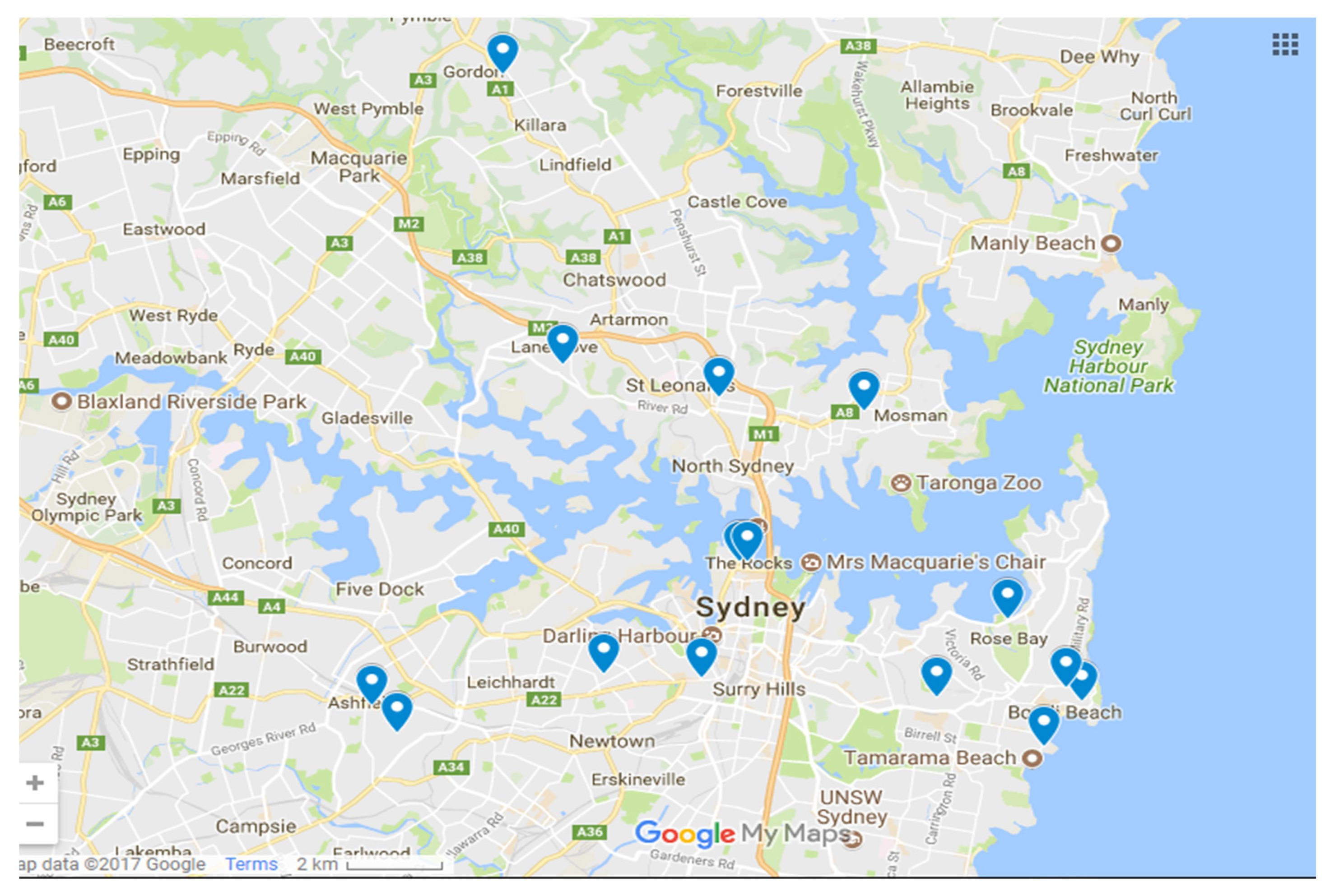
2.1. Measurement Sites

Twelve sites within the urban Sydney region were selected based on the presence of structurally similar outdoor green walls. The sites varied in location, use, and pollutant conditions (Table 1; Figure 1; Appendix Table A1).
Sydney, Australia has a population of 5.2 million and lies on a coastal lowland plain between the Pacific Ocean and elevated sandstone tablelands. Sydney’s climate is warm and temperate, and rainfall is fairly evenly distributed throughout the year. Sydney city’s air quality is generally comparatively good, although PM exceeds the national standards on occasion, especially during bushfires. Noise pollution in Sydney is of concern, with Sydney having the highest traffic related noise exposure amongst Australian cities.

2.2. Measurement Method

Air quality, traffic density, noise and temperature assessments were conducted monthly for 6 consecutive months at all sites between June 2017 and November 2017. The order in which sites were sampled was randomised amongst months to eliminate systematic variation. Samples were taken at green walls and reference walls on the same visit, within 30 min of one another. Samples were not taken on rainy days, as rainfall removes PM from the air [54], and no bare soil was present within 30 m of the sampling locations so as to not artificially spike ambient PM concentrations. Average monthly weather variables were collected for each site using Australian Bureau of Meteorology data to account for weather dependent correlations with in situ conditions. Green wall area and plant number were also recorded for inclusion in the statistical analysis.
At each site, a reference wall was selected based on the following criteria: the reference wall was exposed to the same traffic pollution source as the green wall; the reference wall had similar building characteristics to the green wall, and the reference wall was within 10 m of the green wall. These criteria were used in an attempt to eliminate confounding influences effecting the variables between wall types.
PM measurements were conducted using a DustTrack II 8532 laser densitometer (TSI, Shoreview, MN, USA; sensor type: 90° light scattering, accuracy: ±5%). At each site, time weighted averages for two PM size fractions (particulates <10 µm in diameter—PM10; and particulates <2.5 µm in diameter—PM2.5) were collected between 10:00 a.m. and 3:00 p.m. at both green wall and reference wall locations at each site. At each site location and for each wall type, one 3 min time weighted average sample was collected (an average of each air reading taken per second for 3 min). This was done once per month for a 6-month duration. Samples were taken at 1.5 m above ground, and 0.5 m from the walls.
Traffic density was predicted to be the predominant PM source at all sites. Most sites were situated near residential properties, academic institutes or highways; away from industrial sources of pollutant emissions other than minor infrastructure work. Traffic density was quantified at the closest intersection to the sites for a 30 min duration, each month. Days of the week and times at which air quality and traffic density tests were conducted were limited to weekdays between 10:00 a.m. and 3:00 p.m. to avoid peaks caused by work and school commuters and randomized amongst sites and months [29].
Noise and temperature readings were taken at four point sources across both the green and reference walls at each site using a Digitech Multifunction Environment Meter (sensor type: thermo and audio sensor; accuracy: ±1.2%). The temperature of the ambient air was measured 0.5 m from both wall types. The average and standard error were then determined from the point samples.

2.3. Statistical Analysis

Mean values were calculated for PM2.5, PM10, noise, temperature, and traffic for each month of the study at each site. For use in subsequent analysis, differences between the reference walls and the green walls (henceforth ∆ values) for PM2.5, PM10, noise and temperature were calculated as the (reference wall value—green wall value), so that higher values of ∆ indicate higher PM, noise or temperature levels at reference walls relative to the green walls. Prior to analysis, ∆ PM2.5 and ∆ PM10 were square root transformed to satisfy the assumptions of the models, with a negative sign given to untransformed values less than zero. After transformation, observations retained their original sign (i.e., positive values were not made negative, and vice versa), while decreasing the deviation of the ∆ PM values.
To test if a systematic difference in ambient PM concentrations existed between the green and reference walls, one-tailed paired-sample t-tests were used. Following this, the relationship between ∆ PM2.5 and ∆ PM10 was tested using a linear mixed model regression (LMM) with ∆ PM10 as the response, and ∆ PM2.5 as the predictor variable, with a random slope between ∆ PM2.5 and ∆ PM10 and a random intercept fitted for each site. Site level differences in ∆ PM were then examined, by fitting a linear model to the ∆ PM data and using site as predictor (categorical fixed factor, 13 levels). Using a joint test, the coefficients produced by this model were then tested for differences from zero. Finally, to understand the relationship between PM and environmental factors, multiple regression models of green wall PM2.5 and PM10, and ∆ PM2.5 and ∆ PM10 were built using traffic density, wind, humidity, green wall size, and the number of plants used in the green walls as predictors. Here, LMMs were again employed, with a random intercept fitted for each site.
Using a similar approach to that for PM, overall differences in noise and temperature between green and reference walls were first tested using one-tailed, paired t-tests. Site level differences from zero in ∆ noise and ∆ temperature were then tested by fitting a linear model to each response using site as predictor (categorical fixed factor, 13 levels). Where the joint test of these models was significant, the coefficients from the models were tested for differences from zero to determine which site or sites generated the difference.
All analyses and visualisation were performed in R 3.6.1 (R Core Team 2014, Vienna, Austria), using the packages lme4 [55], lmerTest [56], emmeans [57], and car [58]. Where LMMs were used and models did not include categorical terms, degrees-of-freedom were approximated using the Satterthwaite method for t-tests, while LMMs containing categorical terms used Wald Chi-square tests to generate ANOVA tables.

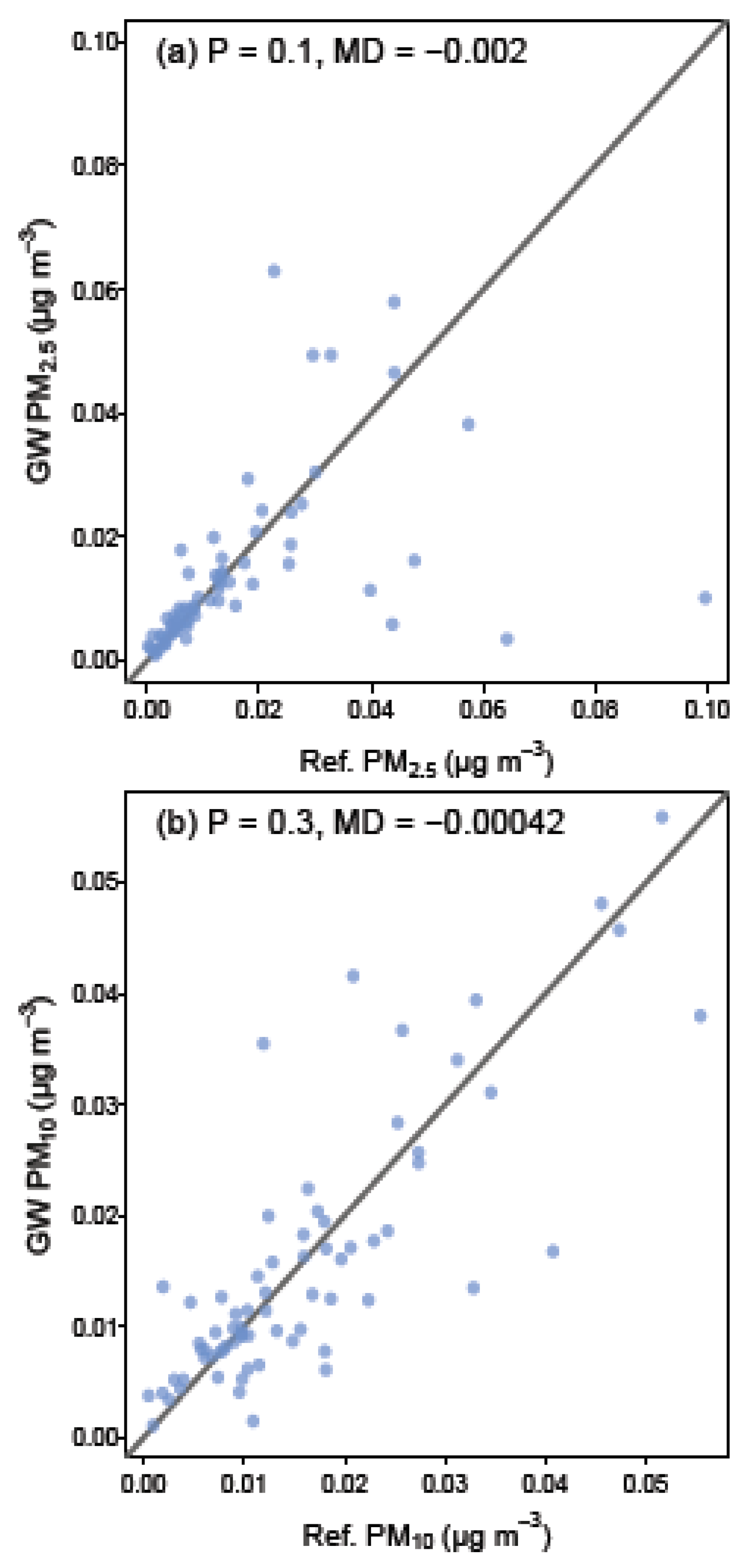
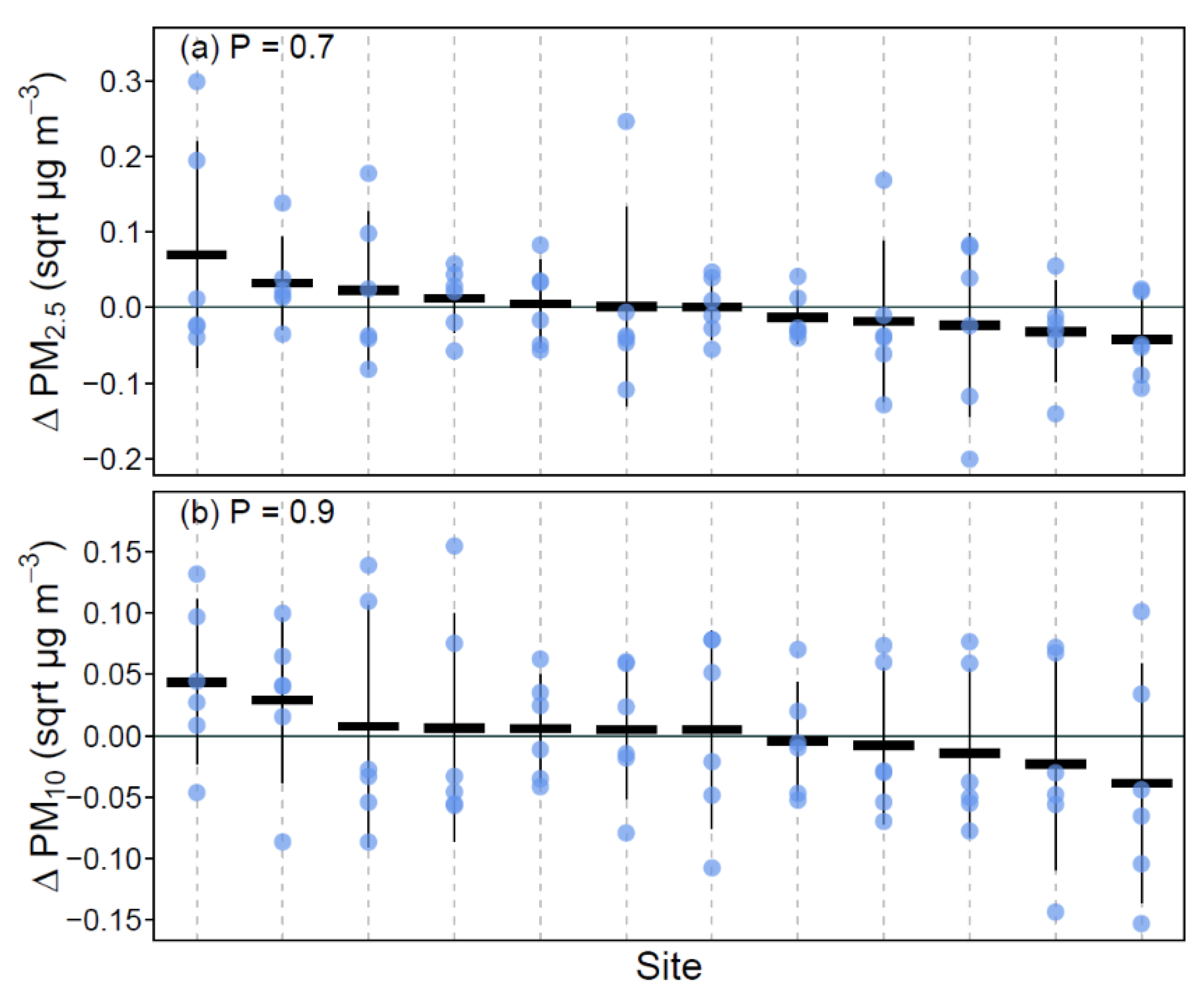
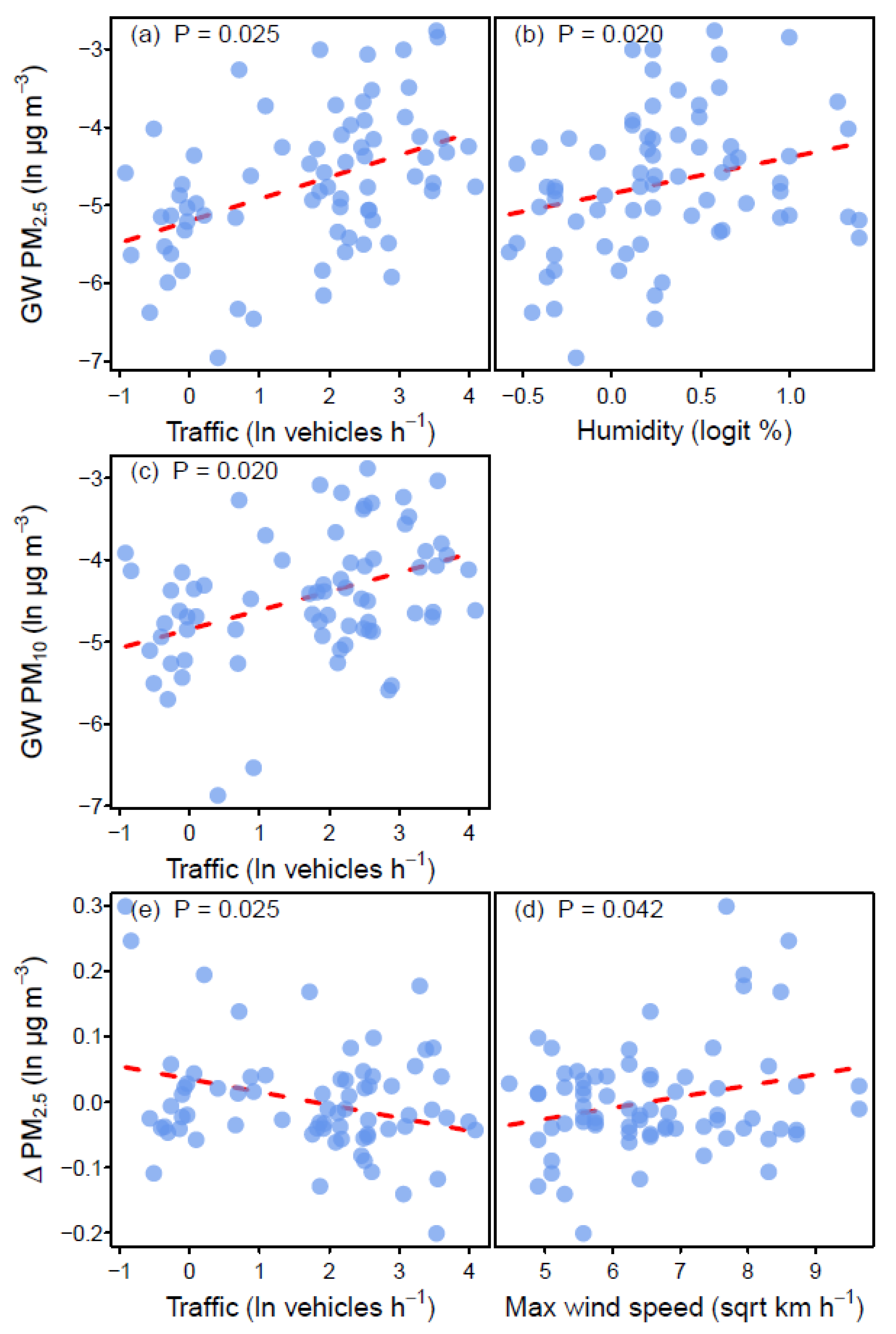
3. Results & Discussion

3.1. Differences in PM Concentration between Wall Types

The ambient PM concentrations at green wall and reference wall locations are presented in Figure 2. Average PM concentrations at the green wall sites were not significantly lower than those recorded at the paired reference walls for PM2.5 (t71 = −1.10, p = 0.1; Figure 2a), nor PM10 (t71 = −0.50, p = 0.3; Figure 2b). Additionally, no significant association between ∆ PM2.5 and ∆ PM10 was found (t10.4 = 1.93, p = 0.08; Figure 2). The common method for determining PM reductions in previous research has been computational modelling, making comparisons with the current in situ results difficult. To the authors’ knowledge, there are no standard methodological guidelines surrounding in situ PM monitoring, and qualifications for what is required by ‘reference walls’. As such, it is unknown whether the 10 m distance between the green wall and reference wall locations was sufficient to observe PM reductions specific to the green walls. Furthermore, it was not appropriate to compare green and reference walls that were any further than 10 m apart as both traffic source and building type altered too significantly at these greater distances, which would have confounded PM comparisons. It is nevertheless suggested that future studies use greater distances between wall types if it is possible to maintain representative conditions over such distances. Whilst it is very likely that there would be a strong relationship between green wall PM efficiency and distance from the wall surface, the current work standardized sampling at 0.5 m from each wall type as distances further than this would have resulted in monitoring in the middle of busy roads at many sites. PM deposition however, has been previously found to be unrelated to differing heights [33] and as such PM was monitored at normal chest height.
This result was surprising, as previous green wall studies have predicted high pollutant removal capacities [27,35,59]. This removal capacity is thought to be due to leaves creating turbulence, forcing compaction between aerosolized PM particles, leading to deposition and eventual accumulation of PM on the leaf surfaces [27,60]. Whilst some PM accumulation was apparent in the current study from visual inspection of the leaves, it is clear that the level of PM removal exhibited had a general effect on proximal air quality that was too small to be detected using the current method, as has been the case in some previous work [61].
The inability of our methods to detect PM removal may have been related to the characteristics of our reference samples. Solid walls have pollution dispersion patterns that may be of similar magnitude to green walls [62,63], with structures such as noise barriers and low boundary walls being shown to have quantifiable effects on proximal air quality [64]. It is also possible that the proximity of the green and reference walls at all sites was such that the influence of the green walls on ambient air quality was sufficient to affect the matched reference sites. It is thus suggested that further studies aim to examine the spatial extent to which air pollution mitigation effects range from their sinks, especially when novel systems are being tested. Alternatively, before–after studies may be of value, as has been proposed previously [27]. Controlling for temporal effects with such methods, however, will be challenging. Due to this limitation, some previous studies have used wind-tunnel and/or modelling trials to replicate before-and-after comparisons e.g., [65]; albeit with limited ability to replicate key in situ influences such as weather and traffic patterns [27].
Currently, claims for significant pollution removal by green walls are matched by many that propose that the effect of urban vegetation on local air pollution mitigation has been exaggerated [66,67,68,69,70]. Thus, there clearly remains uncertainty regarding the pollutant removal capacity of green walls, and as such, further studies are required to identify the true role vegetation plays on local air pollution mitigation [71].
Whilst the current study detected no significant PM removal by green walls, previous controlled laboratory trials [72,73,74,75] have shown that PM, volatile organic compounds (VOCs) and CO2 can be removed at a considerably greater efficiency with the conversion of passive green walls to active systems. Active green wall systems utilise assisted aeration using some form of mechanical fan to actively force air through the plant root and substrate membrane [76]. This leads to an increased surface area for PM adherence, leading to PM entrapment within the substrate and plant root matrix, thus filtering the air more effectively than through the simple diffusion mechanisms on which passive systems are reliant [77,78,79]. Therefore, it is suggested that future studies focus on the potential effect active green wall systems have on ambient PM conditions in situ.
Site-specific PM patterns were investigated to determine if any site-specific PM sources were influential on the relationships observed between PM at the green walls and reference wall locations at each site. This analysis indicated that there was no significant difference from zero found in ∆ PM2.5 amongst sites (F12,60 = 0.72, p = 0.7; Figure 3a), with similar results for ∆ PM10 (F12,60 = 0.52, p = 0.9; Figure 3b). These findings are likely due to the relatively stable pollution conditions within central Sydney.
As ambient conditions, such as traffic and weather patterns, have been previously shown to have an influence on PM conditions, monthly traffic density and weather variables were recorded at each site. Analysis of these data indicated that higher green wall PM2.5 was significantly related to both greater traffic density and higher humidity (Table 2; Figure 4), while higher green wall PM10 was related only to traffic density (Table 2; Figure 4). This result was not surprising, as traffic density is well known to influence air pollution conditions [71,80]. A significant association between lower ∆ PM2.5 and heavier traffic, and higher maximum wind speed was found (Table 2; Figure 4), indicating that both these factors may affect the detectable pollutant removal effect of green walls, as has been found previously in pollutant distribution studies e.g., [65].

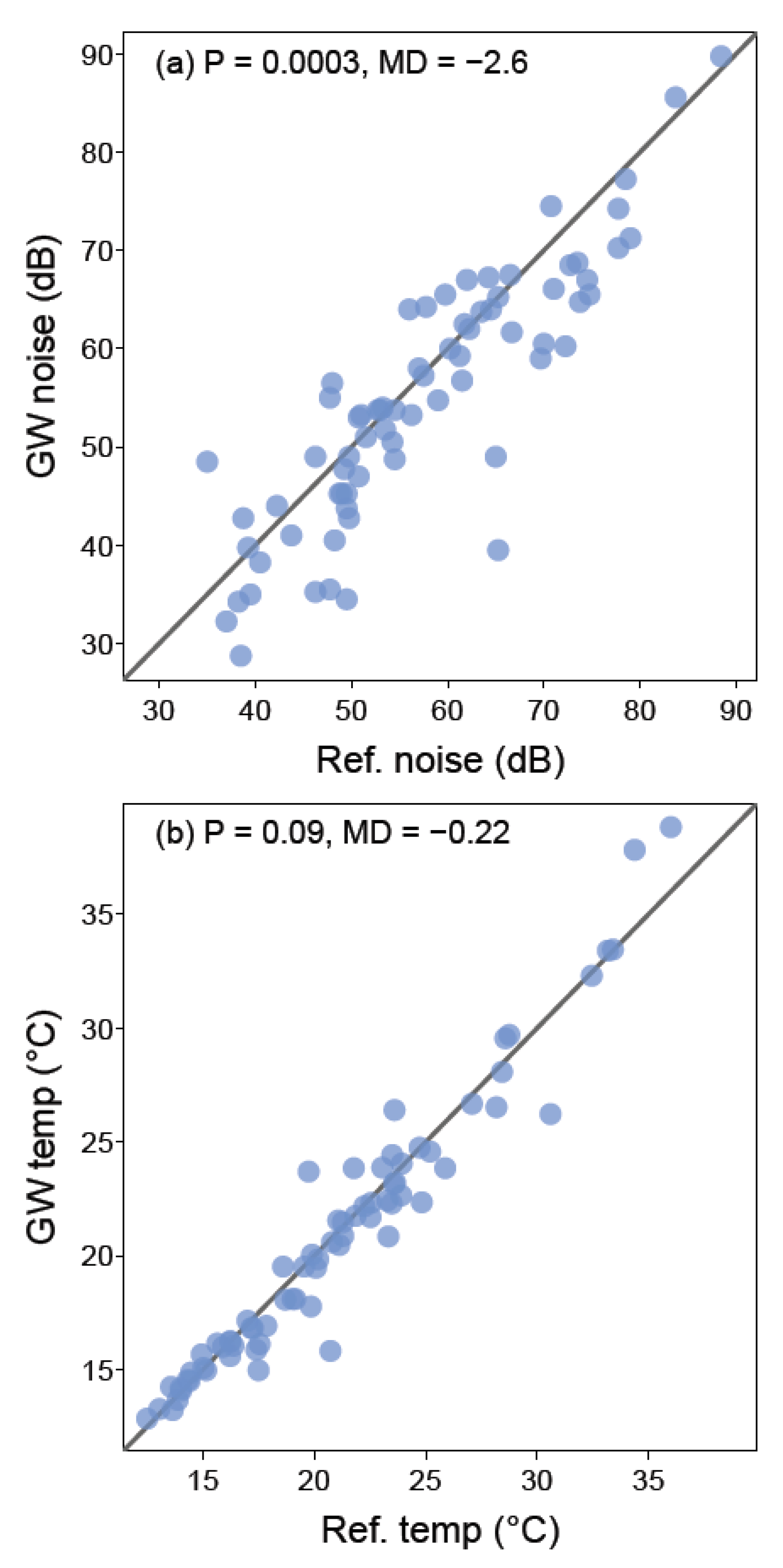
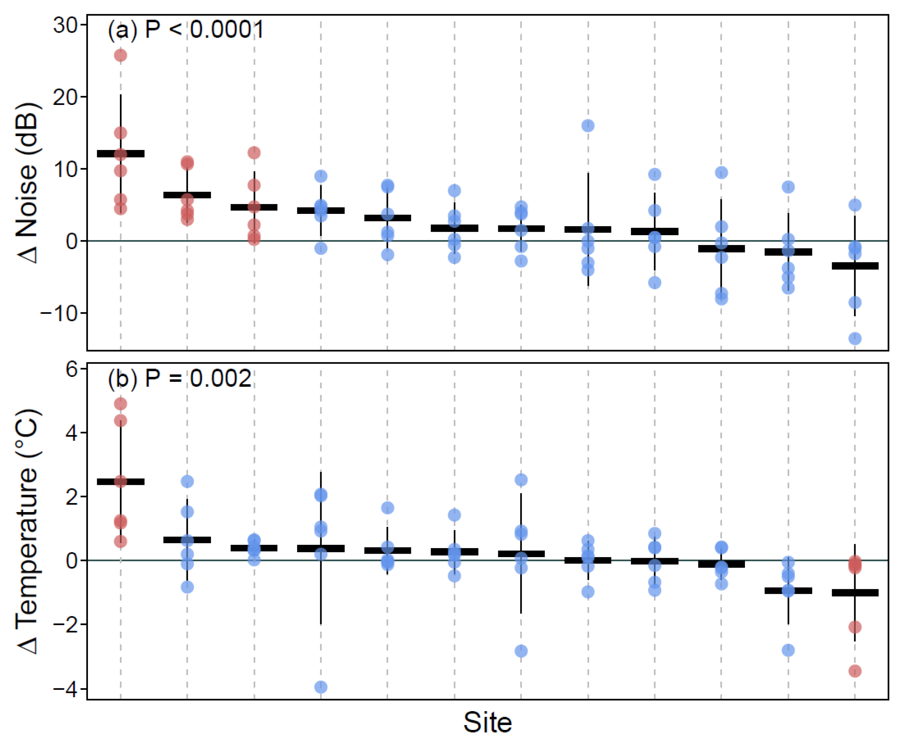
3.2. Differences in Noise and Temperature Conditions between Wall Types

Ambient noise was significantly lower proximal to the green walls relative to their paired reference sites (t71 = −3.55, p = 0.0003; Figure 5a), while no significant difference in temperature was found between treatment groups (t71 = −1.34, p = 0.1; Figure 5b).
Whilst the capacity of green walls to reduce urban noise is still not well understood [7], it is known that plants can absorb noise more effectively than most hard surfaces, which reflect noise of all wavelengths [24,81]. Previous modelling studies have predicted the noise reduction capacity of green walls, estimating that they can reduce 2–5 dB (A) of single point source noises [82], and up to 1.6 dB (A) of road traffic noise [83]. The modelling study conducted by [84] predicted that green walls could reduce emergent and traffic noise by up to 10 dB (A). Klingberg et al. [71] found that traffic noise reduction was proportional to depth of vegetation through which the sound passed, with reductions of 0.6–2.3 dB recorded, a lower range than the site/month average of 1.34–6.40 dB detected in the current work. Interestingly, the maximum noise reduction observed in the current study was 12.13 dB, with this extreme value likely due to the specific and unusual noise type experienced in that sample (ocean related noise, i.e., waves crashing) compared to the predominantly traffic related noise at the other sites.
No significant temperature differences were observed in the current study between the green wall and reference walls, a surprising finding as plants are known to have an air cooling capacity resulting from evapotranspiration. However, whilst [85] recorded temperature reductions of 0.8–4.8 °C from an active green wall, and most indoor green wall studies have demonstrated significant effects on temperature [86,87], outdoor temperature reduction studies have produced variable findings. The work conducted by Alspach and Göhring [88], has indicted that green walls induced temperature reductions of up to 10 °C, with effects strongest in built environments with a height to width ratio greater than 2, which includes dense urban cities such as Melbourne and Hong Kong [52]. It is therefore possible that the building characteristics and unorthodox grid street design of Sydney precluded significant temperature reductions to be recorded in the current work. Alternatively, [89] noted that peak temperature reductions more significant than average reductions, with the effect being of most benefit during extreme heat waves. In the current study, peak temperature reductions were also observed; however, the reductions became non-significant when averaged across sites and months. As such, whilst the green walls within the current study were not effective at consistently reducing ambient temperatures, they still provided occasional peak reductions over the sampling period, and thus may provide benefits in variable climates such as those experiences in Sydney’s Summer periods.
Across sites, it was found that both ∆ noise (F12,60 = 4.82, p < 0.0001) and ∆ temperature (F12,60 = 3.02, p = 0.002) significantly differed from zero. At the site level, ∆ noise was found to be significantly greater than zero at four sites (i.e., noise at green wall sites was lower relative to the reference wall; Figure 6a), while ∆ temperature showed more equivocal results, with one site exhibiting ∆ temperature significantly more than zero, and one other site having ∆ temperature significantly less than zero (Figure 6b).

4. Conclusions

This study assessed the capacity of in situ passive green walls to reduce ambient PM pollution and noise, and to influence proximal temperature. No significant differences were observed between PM concentrations at the green wall and reference wall locations across the 12 sites; indicating that the current passive systems were not capable of reducing PM conditions to a level detectable by the methods used here. The green wall sites tested in the current study, however, had significantly lower proximal noise levels compared to the reference wall sites, indicating that the plants appeared to be absorbing ambient noise. Proximal ambient temperatures at the green wall and reference wall locations were not significantly different. It is thus possible that some previous studies that have used computational modelling procedures to predict major temperature and PM reductions from green walls may have overestimated the in situ effects.

Author Contributions

Conceptualization, N.P., F.T., and P.I.; Methodology, N.P., F.T., and P.I.; Software, D.K.; Formal analysis, D.K.; Writing—original draft preparation, N.P.; Writing—review and editing, N.P., F.T., and P.I.; Supervision, F.T. and P.I. All authors have read and agreed to the published version of the manuscript.

Funding

This research received no external funding.

Acknowledgments

The authors would like to thank Technical staff: Gemma Armstrong, Sue Fenech, Rod Hungerford Paul Brooks, and Helen Price. Research assistants: Ember Liu, Jarrad Climpson, Lincoln de Haas, Tash Bartels, Camilo Perez, Kate Barker, Max Colvin, Quentin Liutai, Edward Hunt, Sarah Walkom, Thomas Churchin, Cadan Jones, Bernice Datu, Hamna Ahmad, Mackenzie Llyod, Cara Gray, Danyon Dowton, Cooper Rispin, Nicholas Hubbard, Kristel Senarillos, Betty Mekonnen, Divya Padavala, Victor Rae, Jarrod Briggs, Sarah Williams, Sandra Sabbagh, Koray Bugdayli, Ashley Bali, Yumna Rehman, Tom O’Neil, Bhavika Kumar, Jeevita Tan, Betina Ferreira, Priyeshi Fernando, Liam Foster Constable, Elena Mel, Rachel Wong, Julia Fyvie-Neill, Samuel Relf, Therese Pace, Carolina Sanchez, and Riley Hughes. Peter J. Irga is financially supported by the UTS Chancellor’s Postdoctoral Research Fellowship scheme (CPDRF), facilitated through The Centre for Technology in Water and Wastewater (CTWW).

Conflicts of Interest

The authors declare no conflict of interest.

Appendix A

Table A1. Test sites with a visual aid.
Site NumberSite LocationPicture
1Ashfield Ijerph 17 05084 i001
2Tamarama Ijerph 17 05084 i002
3Mosman Ijerph 17 05084 i003
4Lane Cove Ijerph 17 05084 i004
5Woollahra Ijerph 17 05084 i005
6Gordon Ijerph 17 05084 i006
7The Rocks, Site 1 Ijerph 17 05084 i007
8The Rocks, Site 2 Ijerph 17 05084 i008
9Summer Hill Ijerph 17 05084 i009
10Camperdown Ijerph 17 05084 i010
11Ultimo Ijerph 17 05084 i011
12Crows Nest Ijerph 17 05084 i012

References

  1. How Much Energy Does NYC Waste? State of the Planet. Available online: https://blogs.ei.columbia.edu/2015/09/28/how-much-energy-does-nyc-waste/ (accessed on 16 September 2019).
  2. Galea, S.; Freudenberg, N.; Vlahov, D. Cities and population health. Soc. Sci. Med. 2005, 60, 1017–1033. [Google Scholar] [CrossRef] [PubMed]
  3. Speak, A.F.; Rothwell, J.J.; Lindley, S.J.; Smith, C.L. Urban particulate pollution reduction by four species of green roof vegetation in a UK city. Atmos. Environ. 2012, 61, 283–293. [Google Scholar] [CrossRef]
  4. Przybysz, A.; Sæbø, A.; Hanslin, H.M.; Gawron’ski, S.W. Accumulation of particulate matter and trace elements on vegetation as affected by pollution level, rainfall and the passage of time. Sci. Total Environ. 2014, 481, 360–369. [Google Scholar] [CrossRef] [PubMed]
  5. Weber, F.; Kowarik, I.; Säumel, I. Herbaceous plants as filters: Immobilization of particulates along urban street corridors. Environ. Pollut. 2014, 186, 234–240. [Google Scholar] [CrossRef] [PubMed]
  6. Air Quality Deteriorating in Many of the World’s Cities World Health Organization. Available online: https://www.who.int/mediacentre/news/releases/2014/air-quality/en/ (accessed on 16 September 2019).
  7. Simunich, J. Background. In Cities Alive Green Building Envelope; Scheuermann, R., Armour, T., Pauli, M., Law, A., Eds.; Arup Deutschland: Berlin, Germany, 2016. [Google Scholar]
  8. Dzierzanowski, K.; Popek, R.; Gawron’ska, H.; Sæbø, A.; Gawron’ska, S.W. Deposition of particulate matter of different size fractions on leaf surfaces and in waxes of urban forest species. Int. J. Phytoremediation 2011, 13, 1037–1046. [Google Scholar] [CrossRef]
  9. Song, Y.; Maher, B.A.; Li, F.; Wang, X.; Sun, X.; Zhang, H. Particulate matter deposited on leaf of five evergreen species in Beijing, China: Source identification and size distribution. Atmos. Environ. 2015, 105, 53–60. [Google Scholar] [CrossRef]
  10. Wang, L.; Gong, H.; Liao, W.; Wang, Z. Accumulation of particles on the surface of leaves during leaf expansion. Sci. Total Environ. 2015, 532, 420–434. [Google Scholar] [CrossRef] [PubMed]
  11. Uttara, S.; Bhuvandas, N.; Aggarwal, V. Impacts of urbanization on environment. Int. J. Res. Eng. Appl. Sci. 2012, 2, 1637–1645. [Google Scholar]
  12. McAlexander, T.P.; Gershon, R.R.M.; Neitzel, R.L. Street-level noise in an urban setting: Assessment and contribution to personal exposure. J. Environ. Health 2015, 14, 1–10. [Google Scholar] [CrossRef] [Green Version]
  13. Scheuermann, R. Introduction, green building envelopes. In Cities Alive Green Building Envelope; Scheuermann, R., Armour, T., Pauli, M., Law, A., Eds.; Arup Deutschland: Berlin, Germany, 2016. [Google Scholar]
  14. Jofeh, C.; Li, J. Retrofitting with Green Envelopes. In Cities Alive Green Building Envelope; Scheuermann, R., Armour, T., Pauli, M., Law, A., Eds.; Arup Deutschland: Berlin, Germany, 2016. [Google Scholar]
  15. Ghazalli, A.J.; Brack, C.; Bai, X.; Said, I. Alterations in use of space, air quality, temperature, and humidity by the presence of vertical greenery system in a building corridor. Urban For. Urban Green. 2018, 32, 177–184. [Google Scholar] [CrossRef]
  16. Sternberg, T.; Viles, H.; Cathersides, A.; Edwards, M. Dust particulate absorption by ivy (Hedera helix L) on historic walls in urban environments. Sci. Total Environ. 2010, 409, 162–168. [Google Scholar] [CrossRef] [PubMed]
  17. Marchi, M.; Pulselli, R.M.; Marchettini, N.; Pulselli, F.M.; Bastianoni, S. Carbon dioxide sequestration model of a vertical greenery system. Ecol. Model. 2015, 306, 46–56. [Google Scholar] [CrossRef]
  18. Charoenkit, S.; Yiemwattana, S. Living walls and their contribution to improved thermal comfort and carbon emission reduction: A review. Build. Environ. 2016, 105, 82–94. [Google Scholar] [CrossRef]
  19. Hasan, M.M.; Karim, A.; Brown, R.J.; Perkins, M.; Joyce, D. Estimation of energy saving of commercial building by living wall and green facade in sub-tropical climate of Australia. In Proceedings of the 7th International Green Energy Conference & the 1st DNL Conference on Clean Energy, Dalian, China, 28–30 May 2012. [Google Scholar]
  20. Mazzali, U.; Peron, F.; Romagnoni, P.; Pulselli, R.M.; Bastianoni, S. Experimental investigation on the energy performance of Living Walls in a temperate climate. Build. Environ. 2013, 64, 57–66. [Google Scholar] [CrossRef]
  21. Coma, J.; Pérez, G.; de Gracia, A.; Burés, S.; Urrestarazu, M.; Cabeza, L.F. Vertical greenery systems for energy savings in buildings: A comparative study between green walls and green facades. Build. Environ. 2017, 111, 228–237. [Google Scholar] [CrossRef] [Green Version]
  22. Cuce, E. Thermal regulation impact of green walls: An experimental and numerical investigation. Appl. Energy 2017, 194, 247–254. [Google Scholar] [CrossRef]
  23. Vox, G.; Blanco, I.; Fuina, S.; Campiotti, C.A.; Mugnozza, G.S.; Schettini, E. Evaluation of wall surface temperatures in green facades. Proc. Inst. Civ. Eng. Eng. Sustain. 2017, 170, 334–344. [Google Scholar] [CrossRef]
  24. Azkorra, Z.; Pérez, G.; Coma, J.; Cabeza, L.F.; Bures, S.; Alvaro, J.E.; Erkoreka, A.; Urrestarazu, M. Evaluation of green walls as a passive acoustic insulation system. Appl. Acoust. 2015, 89, 46–56. [Google Scholar] [CrossRef] [Green Version]
  25. Smith, W.H.; Staskawicz, B.J. Removal of atmospheric particles by leaves and twigs of urban trees: Some preliminary observations and assessment of research needs. Environ. Manag. 1977, 1, 317–330. [Google Scholar] [CrossRef]
  26. Beckett, K.P. Arboriculture: Particle Pollution Removal by Urban Trees; University of Sussex at Brighton: Brighton, UK, 1998. [Google Scholar]
  27. Abhijith, K.V.; Kumar, P.; Gallagher, J.; McNabola, A.; Baldauf, R.; Pilla, F.; Broderick, B.; Di Sabatino, S.; Pulvirenti, B. Air pollution abatement performances of green infrastructure in open road and built-up street canyon environments—A review. Atmos. Environ. 2017, 162, 71–86. [Google Scholar] [CrossRef]
  28. Litschike, T.; Kuttler, W. On the reduction of urban particle concentration by vegetation—A review. Meteorol. Z. 2008, 17, 229–240. [Google Scholar] [CrossRef]
  29. Irga, P.J.; Burchett, M.D.; Torpy, F.R. Does urban forestry have a quantitative effect on ambient air quality in and urban environment? Atmos. Environ. 2015, 120, 173–181. [Google Scholar] [CrossRef] [Green Version]
  30. Al-Dabbous, A.N.; Kumar, P. The influence of roadside vegetation barriers on airborne nanoparticle and pedestrians exposure under varying wind condition. Atmos. Environ. 2014, 90, 113–124. [Google Scholar] [CrossRef] [Green Version]
  31. García-Gómez, H.; Aguillaume, L.; Izquieta-Rojano, S.; Valiño, F.; Àvila, A.; Elustondo, D.; Santamaría, J.M.; Alastuey, A.; Calvete-Sogo, H.; González-Fernández, I.; et al. Atmospheric pollutants in peri-urban forests of Quercus ilex: Evidence of pollution abatement and threats for vegetation. Environ. Sci. Pollut. Res. 2016, 23, 6400–6413. [Google Scholar] [CrossRef] [Green Version]
  32. Beckett, K.P.; Freer-Smith, P.H.; Taylor, G. Particulate pollution capture by urban trees: Effect of species and windspeed. Glob. Chang. Biol. 2000, 6, 995–1003. [Google Scholar] [CrossRef]
  33. Ottelé, M.; van Bohemen, H.D.; Fraaij, A.L.A. Quantifying the deposition of particulate matter on climber vegetation on living walls. Ecol. Eng. 2010, 36, 154–162. [Google Scholar] [CrossRef]
  34. Stevović, S.; Markovic, J. Urban Air Pollutants and Their Impact on Biota. In Plant Responses to Air Pollution; Kulshrestha, U., Saxena, P., Eds.; Springer: Singapore, 2016. [Google Scholar]
  35. Pugh, T.A.M.; Mackenzie, A.R.; Whyatt, J.D.; Hewitt, C.N. Effectiveness of green infrastructure for improvement of air quality in urban street canyons. Environ. Sci. Technol. 2012, 46, 7692–7699. [Google Scholar] [CrossRef] [PubMed] [Green Version]
  36. Joshi, S.V.; Ghosh, S. On the air cleansing efficiency of an extended greenwall: A CFD analysis of mechanistic details of transport processes. J. Theor. Biol. 2014, 361, 101–110. [Google Scholar] [CrossRef] [PubMed]
  37. The Health Effects of Environmental Noise. Available online: https://www1.health.gov.au/internet/main/publishing.nsf/Content/A12B57E41EC9F326CA257BF0001F9E7D/$File/Environmental-health-Risk-Assessment.pdf (accessed on 16 September 2019).
  38. Brown, A.; Bullen, R. Road traffic noise exposure in Australian capital cities. Acoust. Aust. 2003, 31, 11–16. [Google Scholar]
  39. Marquez, L.; Smith, N.; Eugenio, E. Urban Freight in Australia: Societal Costs and Action Plans. Australas. J. Reg. Stud. 2005, 11, 125–139. [Google Scholar]
  40. Traffic Noise Reduction in Europe. Available online: http://www.transportenvironment.org/sites/te/files/media/2008-02_traffic_noise_ce_delft_report.pdf (accessed on 16 September 2019).
  41. How Loud Is It? Available online: http://nymag.com/nymetro/urban/features/noise/9456/ (accessed on 16 September 2019).
  42. Wurm, J. Solar leaf a bioreactive façade. In Cities Alive Green Building Envelope; Scheuermann, R., Armour, T., Pauli, M., Law, A., Eds.; Arup Deutschland: Berlin, Germany, 2016. [Google Scholar]
  43. Embleton, T. Sound propagation in homogeneous deciduous and evergreen woods. J. Acoust. Soc. Am. 1963, 35, 1119–1125. [Google Scholar] [CrossRef]
  44. Martens, M.; Michelsen, A. Absorption of acoustic energy by plant-leaves. J. Acoust. Soc. Am. 1981, 69, 303–306. [Google Scholar] [CrossRef]
  45. Tang, S.; Ong, P.; Woon, H. Monte-Carlo simulation of sound-propagation through leafy foliage using experimentally obtained leaf resonance parameters. J. Acoust. Soc. Am. 1986, 80, 1740–1744. [Google Scholar] [CrossRef]
  46. Van Renterghem, T.; Botteldooren, D.; Verheyen, K. Road traffic noise shielding by vegetation belts of limited depth. J. Sound Vib. 2012, 331, 2404–2425. [Google Scholar] [CrossRef] [Green Version]
  47. Huisman, W.; Attenborough, K. Reverberation and attenuation in a pine forest. J. Acoust. Soc. Am. 1991, 90, 2664–2677. [Google Scholar] [CrossRef]
  48. Martens, M. Foliage as a low-pass filter: Experiments with model forests in an anechoic chamber. J. Acoust. Soc. Am. 1980, 67, 66–72. [Google Scholar] [CrossRef]
  49. Bowler, D.E.; Buyung-Ali, L.; Knight, T.M.; Pullin, A.S. Urban greening to cool towns and cities: A systematic review of the empirical evidence. Landsc. Urban Plan. 2010, 97, 147–155. [Google Scholar] [CrossRef]
  50. Konarska, J.; Uddling, J.; Holmer, B.; Lutz, M.; Lindberg, F.; Pleijel, H.; Thorsson, S. Transpiration of urban trees and its cooling effect in a high latitude city. Int. J. Biometeorol. 2016, 60, 159–172. [Google Scholar] [CrossRef]
  51. Wong, N.H.; Kwang Tan, A.Y.; Chen, Y. Thermal evaluation of vertical greenery systems for building walls. Build. Environ. 2010, 45, 663–672. [Google Scholar] [CrossRef]
  52. Pauli, M. Key Findings. In Cities Alive Green Building Envelope; Scheuermann, R., Armour, T., Pauli, M., Law, A., Eds.; Arup Deutschland: Berlin, Germany, 2016. [Google Scholar]
  53. Pérez, G.; Coma, J.; Martorell, I.; Cabeza, L.F. Vertical Greenery Systems (VGS) for energy saving in buildings: A review. Renew. Sustain. Energy Rev. 2014, 39, 139–165. [Google Scholar] [CrossRef] [Green Version]
  54. Nishihara, T.; Miyaji, T.; Nasu, M.; Takubo, Y.; Kondo, M. Fungal flora in rainwater. Biomed. Environ. Sci. 1989, 2, 376–384. [Google Scholar]
  55. Bates, D.; Maechler, M.; Bolker, B.; Walker, S. Fitting Linear Mixed-Effects Models Using lme4. J. Stat. Softw. 2015, 67, 1–48. Available online: http://arXiv:1406.5823 (accessed on 10 September 2019).
  56. Kuznetsova, A.; Brockhoff, P.B.; Christensen, R.H.B. lmerTest Package: Tests in Linear Mixed Effects Models. J. Stat. Softw. 2017, 82, 1–26. [Google Scholar] [CrossRef] [Green Version]
  57. Estimated Marginal Means, aka Least-Squares Means, R Package Version 1.3.4. Available online: https://CRAN.R-project.org/package=emmeans (accessed on 16 September 2019).
  58. An {R} Companion to Applied Regression, Second Edition. Available online: http://socserv.socsci.mcmaster.ca/jfox/Books/Companion (accessed on 16 September 2019).
  59. Paull, N.J.; Krix, D.; Irga, P.J.; Torpy, F.R. Airborne particulate matter accumulation on common green wall plants. Int. J. Phytoremediation 2019. [Google Scholar] [CrossRef]
  60. Ottelé, M. The Green Building Envelope: Vertical Greening. Ph.D. Thesis, Delft University of Technology, Delft, The Netherlands, 2011. Available online: http://resolver.tudelft.nl/uuid:1e38e393-ca5c-45af-a4fe-31496195b88d (accessed on 16 September 2019).
  61. Setälä, H.; Viippola, V.; Rantalainen, A.L.; Pennanen, A.; Yli-Pelkonen, V. Does urban vegetation mitigate air pollution in northern conditions? Environ. Pollut. 2013, 183, 104–112. [Google Scholar] [CrossRef]
  62. Morakinyo, T.E.; Lam, Y.F.; Hao, S. Evaluating the role of green infrastructures on near-road pollutant dispersion and removal: Modelling and measurement. J. Environ. Manag. 2016, 182, 595–605. [Google Scholar] [CrossRef]
  63. Tong, Z.; Baldauf, R.W.; Isakov, V.; Deshmukh, P.; Max Zhang, K. Roadside vegetation barrier designs to mitigate near-road air pollution impacts. Sci. Total Environ. 2016, 541, 920–927. [Google Scholar] [CrossRef]
  64. Gallagher, J.; Baldauf, R.; Fuller, C.H.; Kumar, P.; Gill, L.W.; McNabola, A. Passive methods for improving air quality in the built environment: A review of porous and solid barriers. Atmos. Environ. 2015, 120, 61–70. [Google Scholar] [CrossRef]
  65. Sanjuan, C.; Bull, M. Green envelopes provide an opportunity to improve air quality in selected areas. In Cities Alive Green Building Envelope; Scheuermann, R., Armour, T., Pauli, M., Law, A., Eds.; Arup Deutschland: Berlin, Germany, 2016. [Google Scholar]
  66. Pataki, D.E.; Carreiro, M.M.; Cherrier, J.; Grulke, N.E.; Jennings, V.; Pincetl, S.; Pouyat, R.V.; Witlow, T.H.; Zipperer, W.C. Coupling biogeochemical cycles in urban environments: Ecosystem services, green solutions, and misconceptions. Front. Ecol. Environ. 2011, 9, 27–36. [Google Scholar] [CrossRef]
  67. Nowak, D.J.; Hirabashi, S.; Bodina, A.; Hoehn, R. Modelled PM2.5 removal by trees in ten U.S. cities and associated health effects. Environ. Pollut. 2013, 178, 395–402. [Google Scholar] [CrossRef] [PubMed]
  68. Whitlow, T.H.; Pataki, D.A.; Alberti, M.; Pincetl, S.; Setala, H.; Cadenasso, M.; Felson, A.; McComas, K. Response to authors’ reply regarding “Modeled PM2.5 removal by trees in ten US cities and associated health effects” by Nowak et al. (2013). Environ. Pollut. 2014, 191, 258–259. [Google Scholar] [CrossRef]
  69. Whitlow, T.H.; Pataki, D.A.; Alberti, M.; Pincetl, S.; Setala, H.; Cadenasso, M.; Felson, A.; McComas, K. Comments on Modelled PM2.5 removal by trees in ten U.S. cities and associated health effects by Nowak et al., (2013). Environ. Pollut. 2014, 191, 256. [Google Scholar] [CrossRef] [PubMed]
  70. Eisenman, T.S.; Churkina, G.; Jariwala, S.P.; Kumar, P.; Lovasi, G.S.; Pataki, D.E.; Weinberger, K.R.; Whitlow, T.H. Urban trees, air quality, and asthma: An interdisciplinary review. Landsc. Urban Plan. 2019, 187, 47–59. [Google Scholar] [CrossRef]
  71. Klingberg, J.; Broberg, M.; Strandberg, B.; Thorsson, P.; Pleijel, H. Influence of urban vegetation on air pollution and noise exposure—A case study in Gothenburg, Sweden. Sci. Total Environ. 2017, 599, 1728–1739. [Google Scholar] [CrossRef] [PubMed]
  72. Torpy, F.R.; Zavattaro, M.; Irga, P.J. Green wall technology for the phytoremediation of indoor air: A system for the reduction of high CO2 concentration. Air Qual. Atmos. Health 2016, 10, 575–585. [Google Scholar] [CrossRef]
  73. Irga, P.J.; Paull, N.J.; Abdo, P.; Torpy, F.R. An assessment of the atmospheric particle removal efficiency of an in-room botanical biofilter system. Build. Environ. 2017, 115, 281–290. [Google Scholar] [CrossRef]
  74. Pettit, T.; Irga, P.J.; Abdo, P.; Torpy, F.R. Do the plants in functional green walls contribute to their ability to filter particulate matter? Build. Environ. 2017, 125, 299–307. [Google Scholar] [CrossRef]
  75. Irga, P.J.; Pettit, T.; Irga, R.F.; Paull, N.J.; Douglas, A.N.J.; Torpy, F.R. Does plant species selection in functional active green walls influence VOC phytoremediation efficiency? Environ. Sci. Pollut. Res. 2019, 26, 12851–12858. [Google Scholar] [CrossRef] [Green Version]
  76. Soreanu, G.; Dixon, M.; Darlington, A. Botanical biofiltration of indoor gaseous pollutants—A mini-review. Chem. Eng. J. 2013, 229, 585–594. [Google Scholar] [CrossRef]
  77. Llewellyn, D.; Dixon, M. Can Plants Really Improve Indoor Air Quality? In Comprehensive Biotechnology, 2nd ed.; Murray, M.Y., Ed.; Academic Press: Burlington, NJ, USA, 2011; pp. 331–338. [Google Scholar]
  78. Veillette, M.; Viens, P.; Ramirez, A.A.; Brzezinski, R.; Heitz, M. Effect of ammonium concentration on microbial population and performance of a biofilter treating air polluted with methane. Chem. Eng. J. 2011, 171, 1114–1123. [Google Scholar] [CrossRef]
  79. Franco, A.; Fernández-Cañero, R.; Pérez-Urrestarazu, L.; Valera, D.L. Wind tunnel analysis of artificial substrates used in active living walls for indoor environment conditioning in Mediterranean buildings. Build. Environ. 2012, 51, 370–378. [Google Scholar] [CrossRef]
  80. Kim, K.H.; Ho, D.X.; Brown, R.J.C.; Oh, J.M.; Park, C.G.; Ryu, I.C. Some insights into the relationship between urban air pollution and noise levels. Sci. Total Environ. 2012, 424, 271–279. [Google Scholar] [CrossRef] [PubMed]
  81. Dunnet, N.; Kingsbury, N. Planting Green Roofs and Living Walls; Timber Press: Portland, OR, USA, 2008. [Google Scholar]
  82. Ismail, M.R. Quiet environment: Acoustics of vertical green wall systems of the Islamic urban form. Front. Arch. Res. 2013, 2, 162–177. [Google Scholar] [CrossRef] [Green Version]
  83. Hosanna Work Package 5 Deliverable 5.7. Technical Report. Available online: http://www.hosanna.bartvanderaa.com/ (accessed on 16 September 2019).
  84. Patel, R.; Boning, W. Acoustics. In Cities Alive Green Building Envelope; Scheuermann, R., Armour, T., Pauli, M., Law, A., Eds.; Arup Deutschland: Berlin, Germany, 2016. [Google Scholar]
  85. Pérez-Urrestarazu, L.; Fernández-Cañero, R.; Franco, A.; Egea, G. Influence of an active living wall on indoor temperature and humidity conditions. Ecol. Eng. 2016, 90, 120–124. [Google Scholar] [CrossRef]
  86. Darlington, A.; Chan, M.; Malloch, D.; Pilger, C.; Dixon, M. The Biofiltration of Indoor Air: Implications for Air quality. Indoor Air 2000, 10, 39–46. [Google Scholar] [CrossRef]
  87. Meier, A.K. Strategic landscaping and air-conditioning savings: Literature review. Energy Build. 2010, 15, 1990–1991. [Google Scholar] [CrossRef]
  88. Alspach, P.; Göhring, A. Urban Heat Island Effect. In Cities Alive, 1st ed.; ARUP Group: Berlin, Germany, 2016; Available online: https://www.arup.com/-/media/arup/files/publications/g/green-building-envelope-report_gesamt_170109.pdf (accessed on 10 September 2019).
  89. Meier, K. Strategic Landscaping and Air-Conditioning Savings: A Green Building Envelope; Scheuermann, R., Armour, T., Pauli, M., Law, A., Eds.; Arup Deutschland: Berlin, Germany, 2016. [Google Scholar]
Figure 1. Spatial distribution of the study sites (image: Google maps).
Ijerph 17 05084 g001
Figure 2. Scatter plots showing concentrations of PM2.5 (a), and PM10 (b) at the green wall (y-axis) and matched reference wall sites (x-axis). The black lines in (a,b) represent 1:1 relationships, therefore all points falling below the line indicate lower values at the green wall relative to the reference wall, and the converse for points above the line. p-values for the paired t-test and the mean difference (MD, green wall value—reference wall value) between paired samples are shown at the top of the graphs.
Ijerph 17 05084 g002
Figure 3. Plots of ∆ PM2.5 (a) and ∆ PM10 (b). Blue points show the ∆ PM values, thick black horizontal lines represent the means for the sites, and thin vertical black lines the 95% confidence interval of the mean for the sites. The p-value at the top of each plot is the result from a joint test of model coefficients with the null hypothesis that the sites do not differ from zero. Sites are sorted on the x-axis by their mean value (highest to lowest) for ease in interpretation. The solid horizontal line indicates zero on the y-axis, representing equal values of PM at the green wall and reference wall.
Ijerph 17 05084 g003
Figure 4. Scatterplots of the significant patterns emerging from the multiple regression models of (a) green wall PM2.5 and traffic, (b) green wall PM2.5 and humidity, (c) green wall PM10 and traffic, (d) ∆ PM2.5 and traffic, and (e), ∆ PM10 and max wind speed. Broken lines are coefficients for the model term of interest, with p-values for the terms shown at top left of each plot.
Ijerph 17 05084 g004
Figure 5. Scatter plots showing noise (a), and temperature (b) at the green wall (y-axis) and reference wall (x-axis). Black lines represent a 1:1 relationship, therefore all points falling below the line indicate lower values at the green wall relative to the reference wall, and the converse for points above the line. In both plots, p-values (paired t-test) and the mean difference (MD, green wall value—reference wall value) between paired samples in shown.
Ijerph 17 05084 g005
Figure 6. Plots of ∆ noise (a) and ∆ temperature (b). Red points are the individual sites that are significantly different from their respective reference sites, and blue points are sites where no significant site-wise differences were observed. Thick black horizontal lines indicate site means, and thin vertical black lines show the 95% confidence interval of the mean for the sites. The p-value at the top of each plot is the result from a joint test of model coefficients with the null hypothesis that the sites do not differ from zero. Sites are sorted on the x-axis by their mean value (highest to lowest) for ease in interpretation. The solid horizontal line indicates zero on the y-axis, representing equal values of noise (a) or temperature (b) at the green wall and reference wall.
Ijerph 17 05084 g006
Table 1. Test site location descriptions
Site NumberSite LocationNotesGeneral Land UseElevation above Sea Level (m)Size (m2)Number of Plants
1Ashfield (33°53′25.7″ S 151°07′40.3″ E)Apartment complex with green wall in outdoor foyerResidential18271296
2Tamarama (33°53′53.5″ S 151°16′23.6″ E)Residential property, green wall situated in back yardResidential3312.5600
3Mosman (33°49′41.7″ S 151°14′04.1″ E)Apartment complex with outdoor green wallResidential and industry70723456
4Lane Cove (33°48′55.8″ S 151°10′10.6″ E)Display home with green wall situated in an outdoor areaIndustry509432
5Woollahra (33°53′15.7″ S 151°14′59.1″ E)Residential property, green wall in front courtyardResidential856288
6Gordon (33°45′33.2″ S 151°09′20.0″ E)High School. Green wall situated in a courtyardResidential1211409150
7The Rocks, Site 1 (33°51′45.6″ S 151°12′20.4″ E)Extensive green wall situated on expresswayTransport191426891
8The Rocks, Site 2 (33°51′39.4″ S 151°12′29.9″ E)Green wall situated under rail line support structureTransport19251600
9Summer Hill (33°53′29.7″ S 151°08′10.2″ E)High School, green wall situated in a courtyardResidential554.5216
10Camperdown (33°53′04.0″ S 151°10′33.8″ E)Multi-storey apartment complexResidential and commercial3018864
11Ultimo (33°53′00.7″ S 151°11′58.0″ E)Green wall situated on a tertiary education facilityEducational151459280
12Crows Nest (33°49′38.3″ S 151°12′07.0″ E)Green wall situated on the exterior of a grocery storeCommercial101251200
Table 2. Results from multiple regression LMMs of green wall PM2.5 and PM10, ∆ PM2.5, and ∆ PM10. Bold p values indicate significant relationship.
ResponseTermsEstimateSEdft Valuep
Green wall PM2.5Traffic0.2810.1017.82.7820.03
Max wind speed−0.1390.07762.2−1.8110.07
Humidity0.4650.19462.32.3910.02
Green wall area−1.1981.2146.4−0.9860.40
Plant number1.1731.1256.41.0420.30
Green wall PM10Traffic0.230.0818.62.8470.02
Max wind speed−0.0980.07364.5−1.3340.20
Humidity0.1970.18564.61.0620.30
Green wall area−0.3890.9557.4−0.4070.70
Plant number0.3330.8857.40.3760.70
∆ PM2.5Traffic−0.020.00966−2.2990.03
Max wind speed0.0170.008662.0760.04
Humidity0.0020.021660.0810.90
Green wall area0.0790.101660.7780.40
Plant number−0.0710.09466−0.7580.50
∆ PM10Traffic0.0040.007660.6280.50
Max wind speed−0.0040.00766−0.4970.60
Humidity0.020.018661.1310.30
Green wall area−0.0530.08866−0.6040.50
Plant number0.050.081660.620.50

