
Analysis and Prediction of Vehicle Kilometers Traveled: A Case Study in Spain

 , ,
, ,
Abstract
:1. Introduction
2. Literature Review
3. Materials and Methods
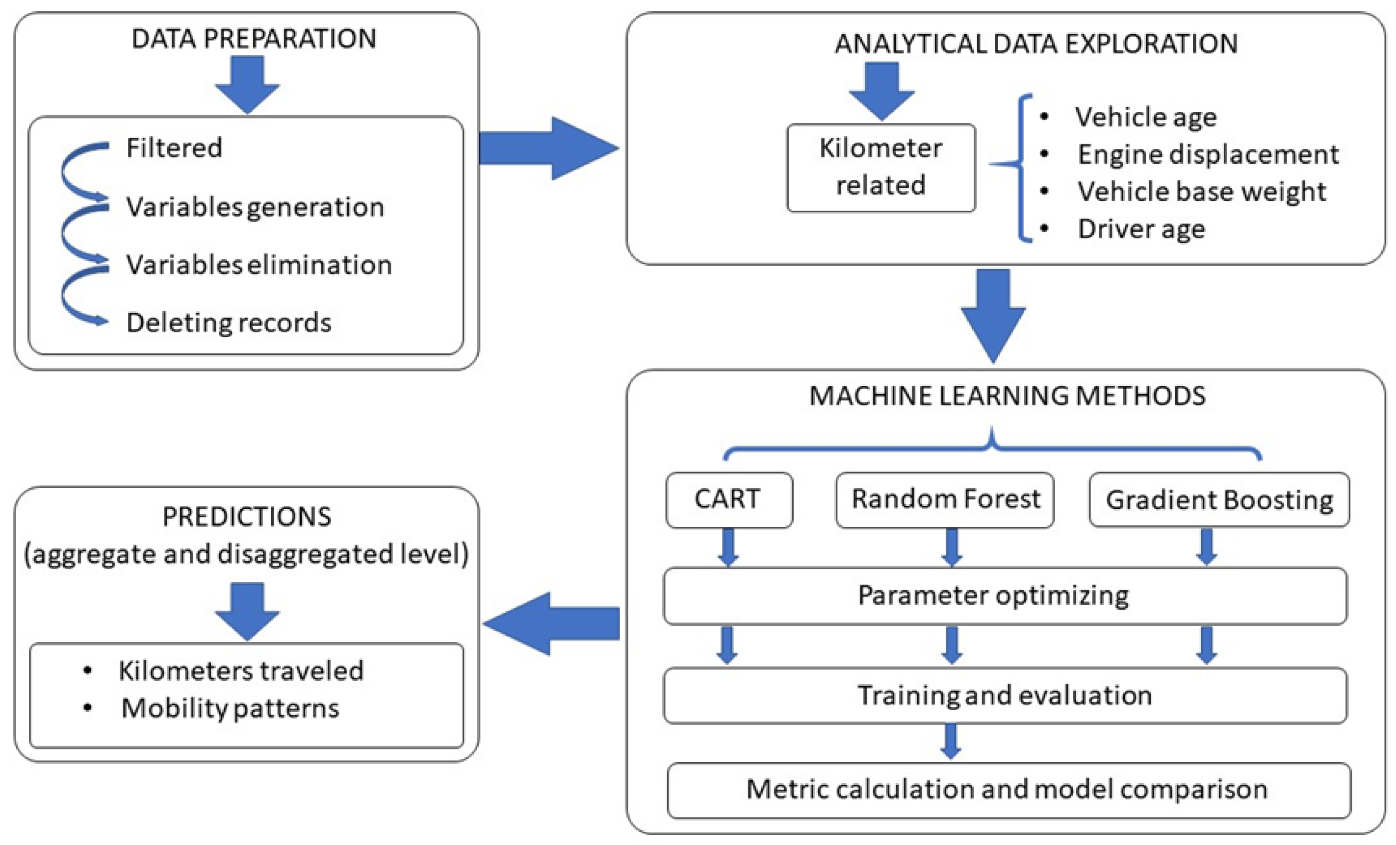
3.1. Methodology: Flow Diagram
3.2. Data Preparation
3.2.1. Raw Data
- Periodicity: this variable indicates the days elapsed between two consecutive inspections; it is calculated from the difference between two consecutive values registered in variable FEC_INSPECCION (ITV date).
- Kilometers traveled (VKT): this variable is determined by (1) where the difference between the odometer reading of the first ITV (X1) and the second reading (X2) is divided by periodicity (Y); this result is multiplied by 365 to obtain the kilometers in annual terms.
- Vehicle age: this variable indicates how old the vehicle is when the inspection is carried out; it is calculated from the difference between the values registered in variable FEC_INSPECCION (ITV date) and FEC_PRIM_MAT (date of first registration).
- Age of the driver: the value of this variable is determined by establishing the age of the owner of the vehicle, with the reasonable assumption that, for passenger vehicles, the owner is the driver. This variable is calculated from the difference between variable FEC_INSPECCION (ITV date) and FEC_NACIMIENTO (date of birth of the owner)
3.2.2. Numerical Summary of the Variables
3.3. Analytical Data Exploration
Univariate Data Analysis
- (1)
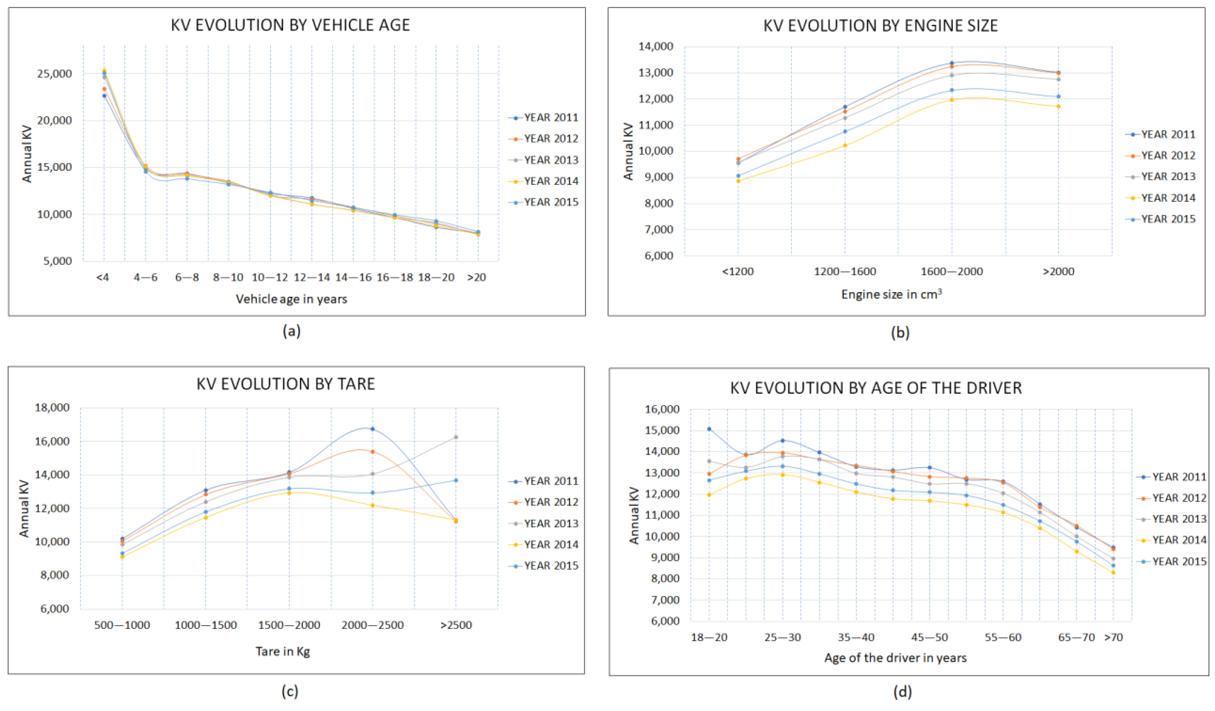
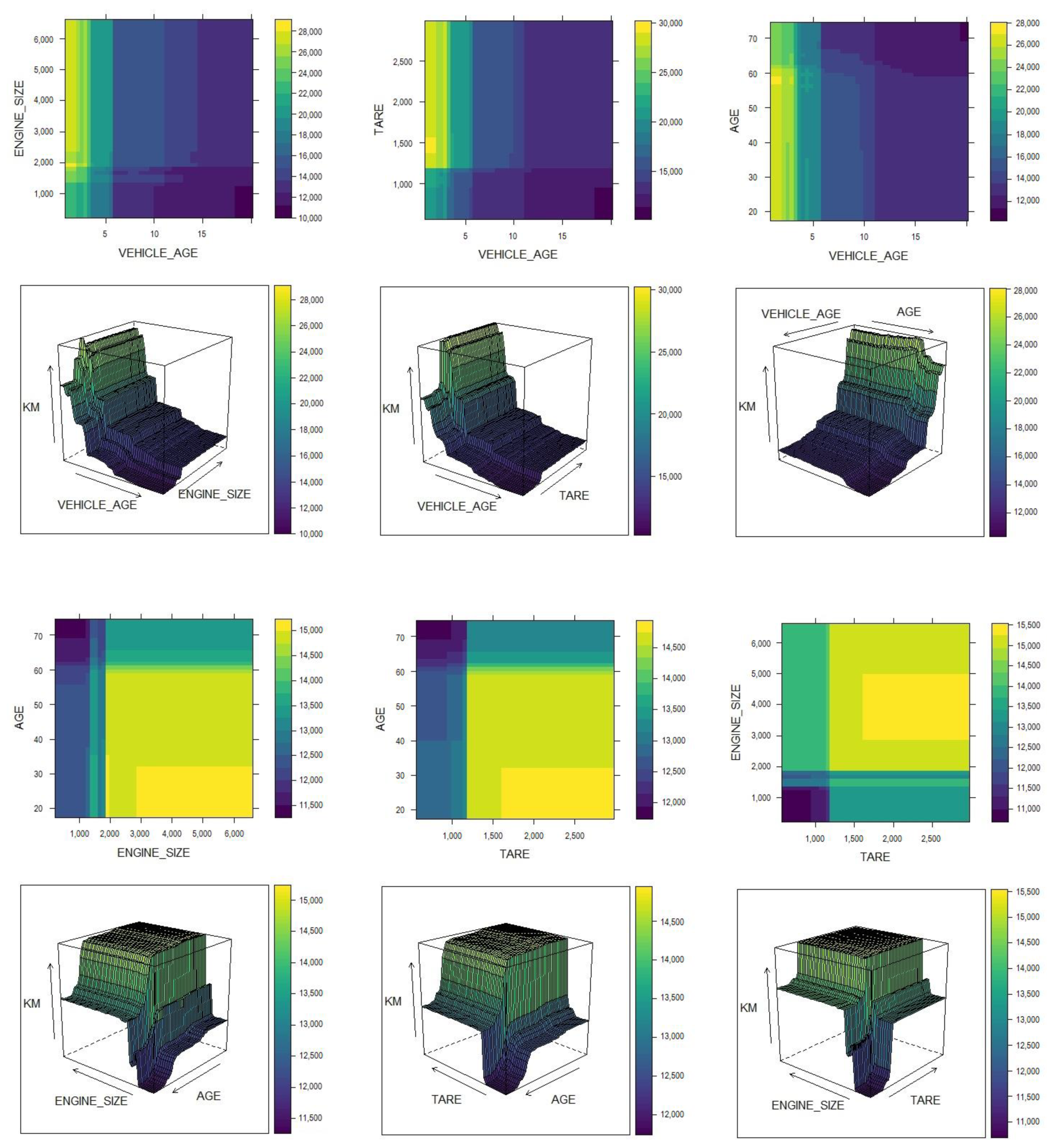
- The relationship between annual VKT and vehicle age shows similar behavior when the data of the five years studied are compared. It is observed that the annual VKT of the vehicles decreases as vehicle age grows, with an inflection point in the range of four to six years. Figure 4a shows two different behaviors in passenger vehicle mobility: one for vehicles up to six years old and another for those over six years old. The rate of mean VKT decline for newer vehicles is higher than for older vehicles. In addition, vehicles less than four years old have approximately twice the VKT of those that are in the 10 to 12 years range and approximately three times that of vehicles older than 20 years;
- (2)
- Figure 4b shows that vehicles with engine size larger than 1600 cm3 have the highest VKT and are in approximately 30% better shape than those with engine size smaller than 1200 cm3, which have the lowest mean VKT value. This information is relevant and reveals a different mobility pattern depending on the composition of the passenger vehicle fleet in terms of engine size, considering that, according to the registration statistics published in DGT (2015), vehicles with an engine size in the range of 1200 to 1600 cm3 represent approximately 54% of the fleet and, if greater than 1600 cm3, approximately 27%;
- (3)
- Vehicles with higher tare weight travel more VKT per year, as Figure 4c shows, which is logical considering that they tend to use engines with greater cubic capacity and higher loads in long routes;
- (4)
- There is a reduction in mobility as the age of the driver increases, as Figure 4d shows. For ages in the range of 25 to 30 years, VKT values slightly higher than the rest are observed, and from ages in the range of 55 to 60 years, there is an increase in the rate at which VKT decline, traveling on average 1000 VKT less for every five-year increase.
3.4. Machine Learning Methods (MLM)
3.4.1. Classification and Regression Tree (CART)
- Start with all the cases in a region, which is the root node.
- At each internal node of the tree, a test is carried out on one of the predictors xj.
- Depending on the test result, the observations are allotted to the left or right subregion (branch) of the tree.
- Step 3 is repeated until reaching a terminal node or leaf in which a prediction is made.
3.4.2. Random Forest (RF)
- For b = 1 to B:
- A size N Bootstrap Z* sample of the training data is drawn.
- An RF tree is grown to the bootstrapped data, recursively repeating the following steps for each node of the tree, until the minimum node nmin is reached.
- Select m variables randomly from the p variables;
- Choose the best variable/split point among m;
- Split the node into two child nodes.
- Exit the set of trees.
3.4.3. Gradient Boosting Model (GBM)
- Select tree depth, D, and the number of iterations, K;
- Compute the average response, ӯ, and use this as the initial predicted value for each sample;
- For k = 1 to K:
- Compute the residuals, the difference between the observed value and the current predicted value for each sample;
- Fit a regression tree of depth D using the residuals as the response;
- Predict each sample using the regression tree fit in the previous step;
- Update the predicted value of each sample by adding the previous iteration’s predicted value to the predicted value generated in the previous step.
- The process ends.
3.4.4. Performance Metrics for Model Comparison
4. Results
4.1. Parameter Optimization
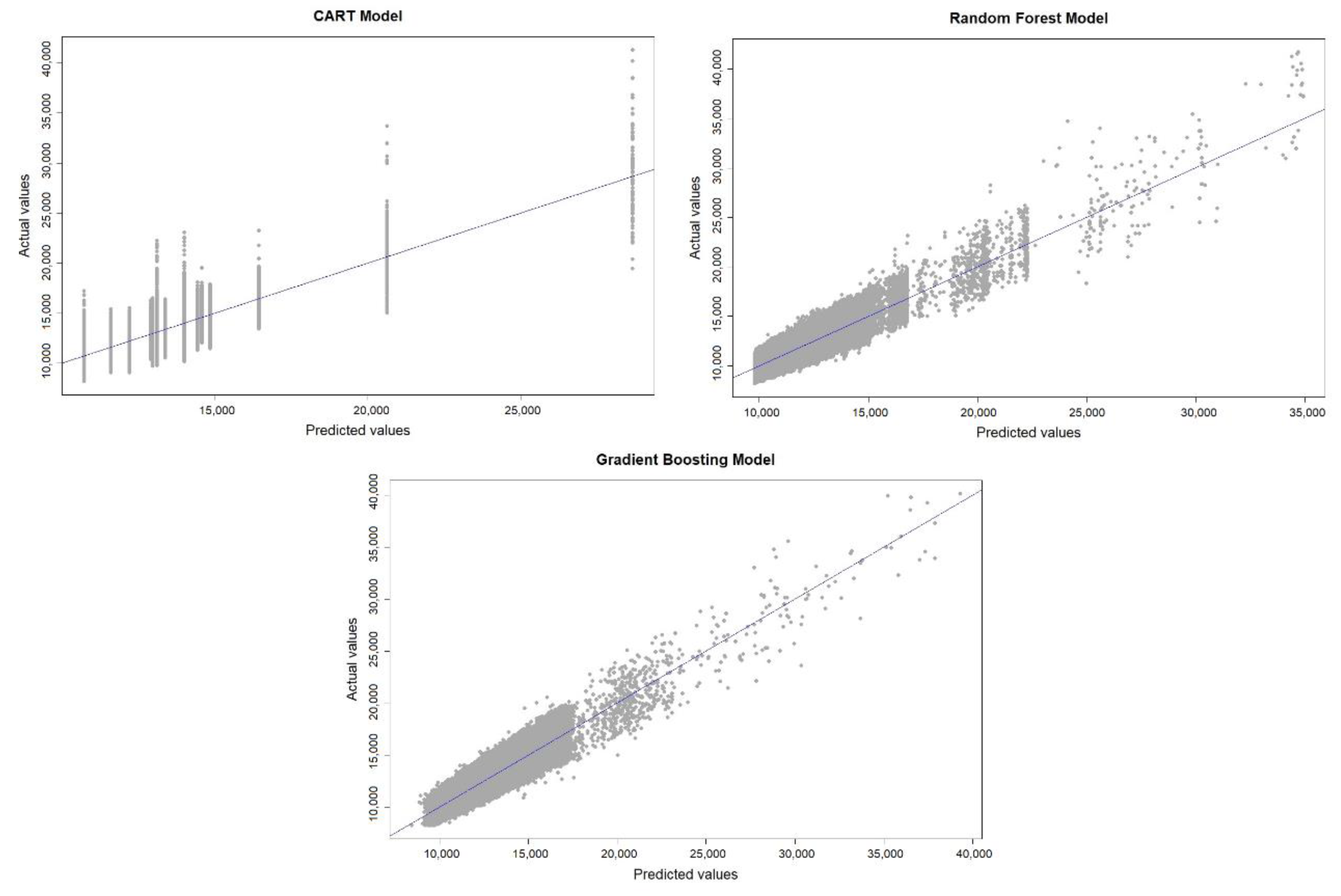
4.2. Performance of Prediction Models
4.3. Prediction and Errors
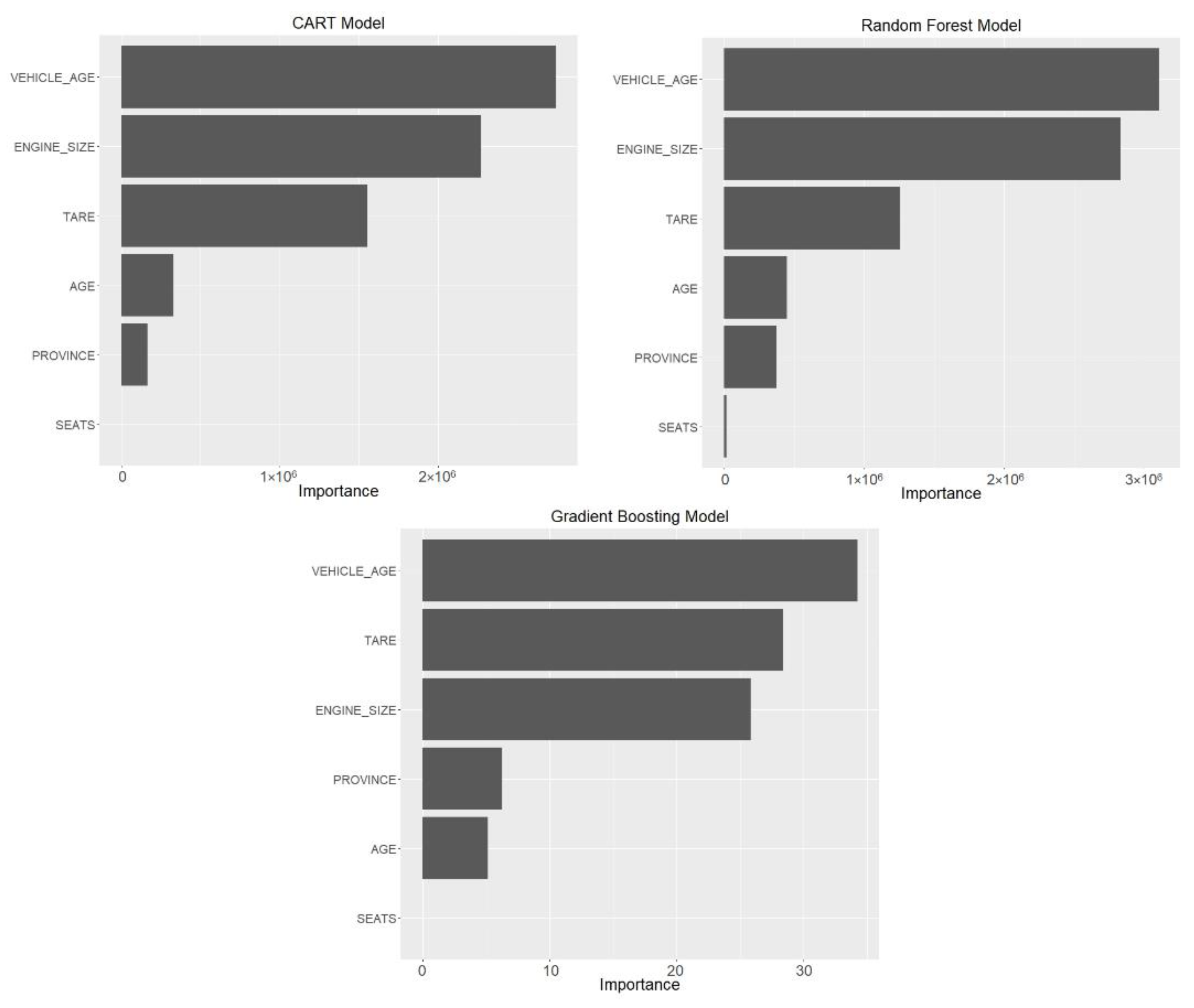
4.4. Variable Importance
4.5. Relevant Pattern Recognition with Selected Machine Learning Models
5. Discussion
6. Conclusions
Author Contributions
Funding
Institutional Review Board Statement
Informed Consent Statement
Data Availability Statement
Acknowledgments
Conflicts of Interest
References
- UNECE. 2015 Statistics of Road Traffic Accidents in Europe and North America. Volume LIII. 2015. Available online: https://www.unece.org/fileadmin/DAM/trans/main/wp6/publications/RAS-2015.pdf (accessed on 23 March 2020).
- Hermans, E.; Wets, G.; Van den Bossche, F. Describing the Evolution in the Number of Highway Deaths by Decomposition in Exposure, Accident Risk, and Fatality Risk. Transp. Res. Rec. 2006, 1950, 1–8. [Google Scholar] [CrossRef]
- Gaudry, M.J.I.; Lassarre, S. Structural Road Accident Models: The International DRAG Family; Emerald Group Publishing Limited: Bingley, UK, 2000; Available online: https://books.google.com.ec/books?id=rhG8wAEACAAJ (accessed on 10 July 2020).
- Gaudry, M. DRAG, un Modèle de la Demande Routière, des Accidents et de leur Gravité, Appliqué au Québec de 1956 à 1982. Ph.D. Thesis, University of Montreal, Montreal, QC, Canada, September 1984. [Google Scholar]
- Izquierdo, F.A.; Ramírez, B.A.; Rodríguez, E.B. The interurban DRAG-Spain model: The main factors of influence on road accidents in Spain. Res. Transp. Econ. 2013, 37, 57–65. Available online: https://0-linkinghub-elsevier-com.brum.beds.ac.uk/retrieve/pii/S0739885911000412 (accessed on 10 July 2021). [CrossRef] [Green Version]
- Dadashova, B.; Ramírez, B.A.; McWilliams, J.M.M.; Izquierdo, F.A. Dynamic Statistical Model Selection: Application to Traffic Accident Analysis in Spain. Procedia Soc. Behav. Sci. 2012, 48, 642–652. [Google Scholar] [CrossRef] [Green Version]
- Gaudry, M.; Himouri, S. DRAG-ALZ-1, a first model of monthly total road demand, accident frequency, severity and victims by category, and of mean speed on highways, Algeria 1970–2007. Res. Transp. Econ. 2013, 37, 66–78. [Google Scholar] [CrossRef]
- Hing, J.Y.C.; Stamatiadis, N.; Aultman-Hall, L. Evaluating the impact of passengers on the safety of older drivers. J. Saf. Res. 2003, 34, 343–351. [Google Scholar] [CrossRef] [PubMed]
- Huggins, R. Using speeding detections and numbers of fatalities to estimate relative risk of a fatality for motorcyclists and car drivers. Accid. Anal. Prev. 2013, 59, 296–300. [Google Scholar] [CrossRef]
- Sagar, S.; Stamatiadis, N.; Wright, S.; Green, E. Use of codes data to improve estimates of at-fault risk for elderly drivers. Accid. Anal. Prev. 2020, 144, 105637. [Google Scholar] [CrossRef]
- Sharmin, S.; Ivan, J.N.; Zhao, S.; Wang, K.; Hossain, M.J.; Ravishanker, N.; Jackson, E. Incorporating Demographic Proportions into Crash Count Models by Quasi-Induced Exposure Method. Transp. Res. Rec. 2020, 2674, 548–560. [Google Scholar] [CrossRef]
- Lardelli-Claret, P.; Luna-Del-Castillo, J.D.D.; Jiménez-Mejías, E.; Pulido-Manzanero, J.; Barrio-Anta, G.; García-Martín, M.; Jiménez-Moleónae, J.J. Comparison of two methods to assess the effect of age and sex on the risk of car crashes. Accid. Anal. Prev. 2011, 43, 1555–1561. [Google Scholar] [CrossRef]
- Martínez-Ruiz, V.; Lardelli-Claret, P.; Jiménez-Mejías, E.; Amezcua-Prieto, C.; Jiménez-Moleón, J.; Luna, J.D. Risk factors for causing road crashes involving cyclists: An application of a quasi-induced exposure method. Accid. Anal. Prev. 2012, 51, 228–237. [Google Scholar] [CrossRef]
- Méndez, Á.G.; Izquierdo, F.A. Quasi-induced exposure: The choice of exposure metrics. Accid. Anal. Prev. 2010, 42, 582–588. [Google Scholar] [CrossRef] [PubMed]
- Pulido, J.; Barrio, G.; Hoyos, J.; Jiménez-Mejías, E.; Martín-Rodríguez, M.D.M.; Houwing, S.; Lardelli-Claret, P. The role of exposure on differences in driver death rates by gender and age: Results of a quasi-induced method on crash data in Spain. Accid. Anal. Prev. 2016, 94, 162–167. [Google Scholar] [CrossRef] [PubMed]
- Chandraratna, S.; Stamatiadis, N. Quasi-induced exposure method: Evaluation of not-at-fault assumption. Accid. Anal. Prev. 2009, 41, 308–313. Available online: http://europepmc.org/abstract/MED/19245890 (accessed on 18 July 2020). [CrossRef] [PubMed]
- Haque, M.M.; Washington, S.; Watson, B. A Methodology for Estimating Exposure-controlled Crash Risk Using Traffic Police Crash Data. Procedia Soc. Behav. Sci. 2013, 104, 972–981. [Google Scholar] [CrossRef]
- Lenguerrand, E.; Martin, J.-L.; Moskal, A.; Gadegbeku, B.; Laumon, B. Limits of the quasi-induced exposure method when compared with the standard case-control design—Application to the estimation of risks associated with driving under the influence of cannabis or alcohol. Accid. Anal. Prev. 2008, 40, 861–868. [Google Scholar] [CrossRef]
- Jiang, X.; Lyles, R.W. Difficulties with quasi-induced exposure when speed varies systematically by vehicle type. Accid. Anal. Prev. 2007, 39, 649–656. [Google Scholar] [CrossRef]
- Jiang, X.; Lyles, R.W. A review of the validity of the underlying assumptions of quasi-induced exposure. Accid. Anal. Prev. 2010, 42, 1352–1358. [Google Scholar] [CrossRef]
- Jiang, X.; Qiu, Y.; Lyles, R.W.; Zhang, H. Issues with using police citations to assign responsibility in quasi-induced exposure. Saf. Sci. 2012, 50, 1133–1140. [Google Scholar] [CrossRef]
- Stamatiadis, N.; Deacon, J.A. Quasi-induced exposure: Methodology and insight. Accid. Anal. Prev. 1997, 29, 37–52. [Google Scholar] [CrossRef]
- Jiang, X.; Lyles, R.W.; Guo, R. A comprehensive review on the quasi-induced exposure technique. Accid. Anal. Prev. 2014, 65, 36–46. [Google Scholar] [CrossRef]
- Ramírez, B.A.; Williams, J.M.M.M.; Fernández, C.G.; Crespo, A.F.; Ayuso, J.P.; Izquierdo, F.A. Metodología Para La Estimación De La Movilidad De Vehículos Del Parque Español. Estudio Piloto: Autobuses Articulados; Editorial Universitat Politècnica de València: Valencia, Spain, 2016. [Google Scholar]
- Izquierdo, F.A.; Sáez, L.M.; Villamor, J.J.H. R&D+I in Automotive: RESULTS. In Proceedings of the First Symposium SEGVAUTO-TRIES-CM. Technologies for a Safe, Accessible and Sustainable Mobility, Madrid, Spain, 17–18 November 2016; Fundación General de la Universidad Politecnica de Madrid: Madrid, Spain, 2016. [Google Scholar]
- Ramírez, B.A. 6o Encuentro con Investigadores Nacionales de Tráfico, Movilidad y Seguridad Vial. Dirección General de Tráfico. 2015. Available online: http://www.dgt.es/images/08-Blanca-Arenas-UPM.pdf (accessed on 14 November 2019).
- Izquierdo, F.A.; Páez, F.; Ramírez, B.A.; Mira, J.; González, C.; Furones, A. Tráfico y Seguridad Vial. Dirección General de Tráfico. 2017. Available online: http://www.dgt.es/revista/num242/mobile/index.html#p=16 (accessed on 14 November 2019).
- Transport Division. Handbook on Statistics on Road Traffic: Methodology and Experience. 2007. Available online: http://www.unece.org/fileadmin/DAM/trans/doc/2007/wp6/handbook_final.pdf (accessed on 11 January 2020).
- Bureau of Infrastructure Transport and Regional Economics. Road vehicle-kilometres travelled: Estimation from state and territory fuel sales. In Proceedings of the Australasian Transport Research Forum 2011, Adelaide, Australia, 28–30 September 2011. [Google Scholar]
- Papadimitriou, E.; Yannis, G.; Bijleveld, F.; Cardoso, J.L. Exposure data and risk indicators for safety performance assessment in Europe. Accid. Anal. Prev. 2013, 60, 371–383. Available online: https://0-www-sciencedirect-com.brum.beds.ac.uk/science/article/pii/S0001457513001954 (accessed on 19 February 2020). [CrossRef]
- Assemi, B.; Hickman, M. Relationship between heavy vehicle periodic inspections, crash contributing factors and crash severity. Transp. Res. Part A Policy Pract. 2018, 113, 441–459. [Google Scholar] [CrossRef]
- Christensen, P.; Elvik, R. Effects on accidents of periodic motor vehicle inspection in Norway. Accid. Anal. Prev. 2007, 39, 47–52. [Google Scholar] [CrossRef] [PubMed]
- Elvik, R. The effect on accidents of technical inspections of heavy vehicles in Norway. Accid. Anal. Prev. 2002, 34, 753–762. [Google Scholar] [CrossRef]
- Malik, L.; Tiwari, G. Assessment of interstate freight vehicle characteristics and impact of future emission and fuel economy standards on their emissions in India. Energy Policy 2017, 108, 121–133. Available online: https://0-www-sciencedirect-com.brum.beds.ac.uk/science/article/pii/S0301421517303440 (accessed on 19 February 2020). [CrossRef]
- Wilson, R.E.; Cairns, S.; Notley, S.; Anable, J.; Chatterton, T.; McLeod, F. Techniques for the inference of mileage rates from MOT data. Transp. Plan. Technol. 2013, 36, 130–143. [Google Scholar] [CrossRef] [Green Version]
- Lee, D.; Guldmann, J.M.; Choi, C. Factors contributing to the relationship between driving mileage and crash frequency of older drivers. Sustainability 2019, 11, 6643. [Google Scholar] [CrossRef] [Green Version]
- Mrozik, M.; Merkisz-Guranowska, A. Environmental assessment of the vehicle operation process. Energies 2021, 14, 76. [Google Scholar] [CrossRef]
- Bharadwaj, S.; Ballare, S.; Rohit, C.M.K. Impact of congestion on greenhouse gas emissions for road transport in Mumbai metropolitan region. Transp. Res. Procedia 2017, 25, 3538–3551. Available online: https://0-www-sciencedirect-com.brum.beds.ac.uk/science/article/pii/S2352146517305896 (accessed on 19 February 2020). [CrossRef]
- Jung, S.; Kim, J.; Kim, J.; Hong, D.; Park, D. An estimation of vehicle kilometer traveled and on-road emissions using the traffic volume and travel speed on road links in Incheon City. J. Environ. Sci. 2017, 54, 90–100. [Google Scholar] [CrossRef]
- Wu, X.; Wu, Y.; Zhang, S.; Liu, H.; Fu, L.; Hao, J. Assessment of vehicle emission programs in China during 1998–2013: Achievement, challenges and implications. Environ. Pollut. 2016, 214, 556–567. [Google Scholar] [CrossRef] [PubMed]
- Núñez-Córdoba, J.M.; Bes-Rastrollo, M.; Pollack, K.M.; Seguí-Gómez, M.; Beunza, J.J.; Sayón-Orea, C.; Martínez-González, M.A. Annual motor vehicle travel distance and incident obesity: A prospective cohort study. Am. J. Prev. Med. 2013, 44, 254–259. [Google Scholar] [CrossRef] [PubMed]
- Bin, O. A logit analysis of vehicle emissions using inspection and maintenance testing data. Transp. Res. Part D Transp. Environ. 2003, 8, 215–227. [Google Scholar] [CrossRef]
- Washburn, S.; Seet, J.; Mannering, F. Statistical modeling of vehicle emissions from inspection/maintenance testing data: An exploratory analysis. Transp. Res. Part D Transp. Environ. 2001, 6, 21–36. [Google Scholar] [CrossRef]
- Beydoun, M.; Guldmann, J.M. Vehicle characteristics and emissions: Logit and regression analyses of I/M data from Massachusetts, Maryland, and Illinois. Transp. Res. Part D Transp. Environ. 2006, 11, 59–76. [Google Scholar] [CrossRef]
- Sancho, S.; Gaja, E.; Peral-Orts, R.; Clemente, G.; Sanz, J.; Velasco-Sánchez, E. Analysis of sound level emitted by vehicle regarding age. Appl. Acoust. 2017, 126, 162–169. [Google Scholar] [CrossRef]
- Hirota, K. Comparative studies on vehicle related policies for air pollution reduction in ten Asian countries. Sustainability 2010, 2, 145–162. [Google Scholar] [CrossRef] [Green Version]
- Keall, M.D.; Newstead, S. An evaluation of costs and benefits of a vehicle periodic inspection scheme with six-monthly inspections compared to annual inspections. Accid. Anal. Prev. 2013, 58, 81–87. [Google Scholar] [CrossRef]
- Faiz, A.; Bahadur, A.B.; Nagarkoti, R.K. The role of inspection and maintenance in controlling vehicular emissions in Kathmandu valley, Nepal. Atmos. Environ. 2006, 40, 5967–5975. [Google Scholar] [CrossRef]
- Wilson, R.E.; Anable, J.; Cairns, S.; Chatterton, T.; Notley, S.; Lees-Miller, J.D. On the estimation of temporal mileage rates. Transp. Res. Part E Logist. Transp. Rev. 2013, 60, 126–139. [Google Scholar] [CrossRef] [Green Version]
- Izquierdo, F.A.; Ramírez, B.A. Desarrollo y Aplicación de Una Metodología Integrada Para el Estudio de los Accidentes de Tráfico con Implicación de Furgonetas. Madrid. 2012, p. 245. Available online: http://insia-upm.es/portfolio-items/proyecto-furgoseg/?lang=en (accessed on 18 November 2019).
- Hong, J.; Shen, Q.; Zhang, L. How do built-environment factors affect travel behavior? A spatial analysis at different geographic scales. Transportation 2014, 41, 419–440. [Google Scholar] [CrossRef]
- Chen, F.; Wu, J.; Chen, X.; Zegras, P.C.; Wang, J. Vehicle kilometers traveled reduction impacts of Transit-Oriented Development: Evidence from Shanghai City. Transp. Res. Part D Transp. Environ. 2017, 55, 227–245. [Google Scholar] [CrossRef]
- Cao, X.; Xu, Z.; Fan, Y. Exploring the connections among residential location, self-selection, and driving: Propensity score matching with multiple treatments. Transp. Res. Part A Policy Pract. 2010, 44, 797–805. [Google Scholar] [CrossRef]
- Zhou, B.; Kockelman, K.M. Self-selection in home choice: Use of treatment effects in evaluating relationship between built environment and travel behavior. Transp. Res. Rec. 2008, 2077, 54–61. [Google Scholar] [CrossRef] [Green Version]
- Duncan, M. Would the replacement of park-and-ride facilities with transit-oriented development reduce vehicle kilometers traveled in an auto-oriented US region? Transp. Policy 2019, 81, 293–301. [Google Scholar] [CrossRef]
- Zolnik, E.J. Effects of additional capacity on vehicle kilometers of travel in the U.S.: Evidence from National Household Travel Surveys. J. Transp. Geogr. 2018, 66, 1–9. [Google Scholar] [CrossRef]
- Goebel, D.; Plötz, P. Machine learning estimates of plug-in hybrid electric vehicle utility factors. Transp. Res. Part D Transp. Environ. 2019, 72, 36–46. Available online: https://0-www-sciencedirect-com.brum.beds.ac.uk/science/article/pii/S1361920918301561 (accessed on 19 February 2020). [CrossRef]
- Wang, S.; Li, Z. Exploring causes and effects of automated vehicle disengagement using statistical modeling and classification tree based on field test data. Accid. Anal. Prev. 2019, 129, 44–54. Available online: https://0-www-sciencedirect-com.brum.beds.ac.uk/science/article/pii/S0001457519300016 (accessed on 19 February 2020). [CrossRef]
- Singh, D.; Nigam, S.P.; Agrawal, V.P.; Kumar, M. Vehicular traffic noise prediction using soft computing approach. J. Environ. Manag. 2016, 183, 59–66. Available online: https://0-www-sciencedirect-com.brum.beds.ac.uk/science/article/pii/S0301479716305916 (accessed on 19 February 2020). [CrossRef]
- Rahman, M.S.; Abdel-Aty, M.; Hasan, S.; Cai, Q. Applying machine learning approaches to analyze the vulnerable road-users’ crashes at statewide traffic analysis zones. J. Saf. Res. 2019, 70, 275–288. Available online: https://0-www-sciencedirect-com.brum.beds.ac.uk/science/article/pii/S0022437518304146 (accessed on 19 February 2020). [CrossRef] [PubMed]
- Williams, G. Data Mining with Rattle and R; Springer: New York, NY, USA, 2011; pp. 21–54. [Google Scholar]
- Friedman, J.; Hastie, T.; Tibshirani, R. The Elements of Statistical Learning; Springer: New York, NY, USA, 2009. [Google Scholar]
- Gong, H.; Sun, Y.; Shu, X.; Huang, B. Use of random forests regression for predicting IRI of asphalt pavements. Constr. Build. Mater. 2018, 189, 890–897. Available online: https://0-www-sciencedirect-com.brum.beds.ac.uk/science/article/pii/S0950061818321937 (accessed on 19 February 2020). [CrossRef]
- Therneau, T.; Atkinson, B.; Ripley, B. Package “RPART”. 2019, p. 34. Available online: https://cran.r-project.org/package=rpart (accessed on 18 February 2020).
- Cheng, L.; Chen, X.; De Vos, J.; Lai, X.; Witlox, F. Applying a random forest method approach to model travel mode choice behavior. Travel Behav. Soc. 2019, 14, 1–10. Available online: https://0-www-sciencedirect-com.brum.beds.ac.uk/science/article/pii/S2214367X18300863 (accessed on 19 February 2020). [CrossRef]
- Dadashova, B.; Ramírez, B.A.; McWilliams, J.M.; Izquierdo, F.A. The Identification of Patterns of Interurban Road Accident Frequency and Severity Using Road Geometry and Traffic Indicators. Transp. Res. Procedia 2016, 14, 4122–4129. Available online: https://0-www-sciencedirect-com.brum.beds.ac.uk/science/article/pii/S2352146516303891 (accessed on 19 February 2020). [CrossRef] [Green Version]
- Theofilatos, A. Incorporating real-time traffic and weather data to explore road accident likelihood and severity in urban arterials. J. Saf. Res. 2017, 61, 9–21. Available online: https://0-www-sciencedirect-com.brum.beds.ac.uk/science/article/pii/S0022437517301378 (accessed on 19 February 2020). [CrossRef]
- Harb, R.; Yan, X.; Radwan, E.; Su, X. Exploring precrash maneuvers using classification trees and random forests. Accid. Anal. Prev. 2009, 41, 98–107. Available online: https://0-www-sciencedirect-com.brum.beds.ac.uk/science/article/pii/S0001457508001887 (accessed on 19 February 2020). [CrossRef]
- Okamoto, K.; Berntorp, K.; Di Cairano, S. Driver Intention-based Vehicle Threat Assessment using Random Forests and Particle Filtering. IFAC PapersOnLine 2017, 50, 13860–13865. Available online: https://0-www-sciencedirect-com.brum.beds.ac.uk/science/article/pii/S2405896317329063?via%3Dihub (accessed on 19 February 2020). [CrossRef]
- Breiman, L. Random forests. Mach. Learn. 2001, 45, 5–32. [Google Scholar] [CrossRef] [Green Version]
- Speiser, J.L.; Miller, M.E.; Tooze, J.; Ip, E. A comparison of random forest variable selection methods for classification prediction modeling. Expert Syst. Appl. 2019, 134, 93–101. Available online: https://0-www-sciencedirect-com.brum.beds.ac.uk/science/article/pii/S0957417419303574 (accessed on 19 February 2020). [CrossRef]
- Wright, M.; Wager, S.; Probst, P. Package “Ranger”. 2020, p. 25. Available online: https://github.com/imbs-hl/ranger (accessed on 18 February 2020).
- Schlögl, M.; Stütz, R.; Laaha, G.; Melcher, M. A comparison of statistical learning methods for deriving determining factors of accident occurrence from an imbalanced high resolution dataset. Accid. Anal. Prev. 2019, 127, 134–149. [Google Scholar] [CrossRef]
- Schlögl, M. A multivariate analysis of environmental effects on road accident occurrence using a balanced bagging approach. Accid. Anal. Prev. 2020, 136, 105398. [Google Scholar] [CrossRef] [PubMed]
- Tang, J.; Liang, J.; Han, C.; Li, Z.; Huang, H. Crash injury severity analysis using a two-layer Stacking framework. Accid. Anal. Prev. 2019, 122, 226–238. [Google Scholar] [CrossRef] [PubMed]
- Zheng, Z.; Lu, P.; Lantz, B. Commercial truck crash injury severity analysis using gradient boosting data mining model. J. Saf. Res. 2018, 65, 115–124. [Google Scholar] [CrossRef] [PubMed]
- Xu, J.; Saleh, M.; Hatzopoulou, M. A machine learning approach capturing the effects of driving behaviour and driver characteristics on trip-level emissions. Atmos. Environ. 2020, 224, 117311. [Google Scholar] [CrossRef]
- Kuhn, M.; Johnson, K. Applied Predictive Modeling; Springer: New York, NY, USA, 2013; pp. 1–600. [Google Scholar]
- Greenwell, B.; Bochmke, B.; Cunningham, J. Package “GBM”. 2019, p. 39. Available online: https://github.com/gbm-developers/gbm (accessed on 11 March 2020).


| Field | Variables: ITV Code (Description) | No. of Records with Zero Value | No. of Empty Records | Percentage of Invalid Records 1 |
|---|---|---|---|---|
| Vehicle identification | newid (Vehicle Identification Code) | 0 | 0 | 0.00% |
| FEC_MATRICULA (Date of registration) | 0 | 0 | 0.00% | |
| COD_CLASE_MAT 2 (Registration class) | 6,258,376 | 0 | 99.49% | |
| JEFATURA_MAT_NORM (Province of registration) | 0 | 0 | 0.00% | |
| COD_MARCA_OBV (Vehicle Make Identification) | 0 | 0 | 0.00% | |
| MODELO_OBV (Model description) | 0 | 218 | 0.00% | |
| COD_TIPO_OBV (Vehicle type) | 0 | 0 | 0.00% | |
| FEC_PRIM_MAT (Date of first registration) | 0 | 0 | 0.00% | |
| RENTING (Rental vehicle) | 0 | 4,878,481 | 77.55% | |
| Technical data | CO2 (CO2 emissions) | 8135 | 6,161,708 | 98.08% |
| TIPO_ALIMENTACION (Fuel type) | 2 | 6,268,947 | 99.65% | |
| CILINDRADA_OBV (Engine size) | 2481 | 0 | 0.04% | |
| POTENCIA_OBV (Tax horsepower of the vehicle) | 3207 | 0 | 0.05% | |
| TARA_OBV (Tare weight) | 2529 | 0 | 0.04% | |
| PESO_MAX_OBV (Maximum weight) | 47,563 | 0 | 0.76% | |
| NUM_PLAZAS_MAX (Maximum number of seats) | 2667 | 0 | 0.04% | |
| MTMA (Maximum Technically Permissible Mass) | 5,114,835 | 0 | 81.31% | |
| MMC (Mass in running order) | 5,079,130 | 0 | 80.74% | |
| KW (Maximum net power) | 5,199,797 | 0 | 82.66% | |
| RPP (Weight power ratio) | 6,267,254 | 0 | 99.63% | |
| CARROCERIA (Bodywork type) | 0 | 6,272,460 | 99.71% | |
| CONSUMO (Fuel consumption) | 6,290,653 | 0 | 100.00% | |
| DISTANCIA_EJES (Wheelbase) | 6,271,015 | 0 | 99.69% | |
| CODIGO_ECO (Eco code) | 0 | 6,290,664 | 100.00% | |
| CATELECT (Electric vehicle) | 0 | 6,285,655 | 99.92% | |
| AUTELECT (Electric vehicle range) | 4494 | 6,286,140 | 100.00% | |
| Ownership | FEC_NACIMIENTO (Date of birth of the owner) | 0 | 356,010 | 5.66% |
| PERSONA_JURIDICA (Legal entity) | 0 | 5,933,259 | 94.32% | |
| Technical inspection history | FEC_INSPECCION (ITV date) | 0 | 844,837 | 13.43% |
| NUM_ITV (Technical inspection number) | 0 | 0 | 0.00% | |
| CLAVE (Vehicle technical inspection result) | 0 | 0 | 0.00% | |
| COD_PROVINCIA (Province of domicile of the vehicle) | 0 | 80 | 0.00% | |
| KM1 (Odometer reading) | 0 | 3,954,130 | 62.86% | |
| History of defects | DESC_GRUPO_DEFECTO_1 (Breakdown location group) | 0 | 5,623,957 | 89.40% |
| DESC_DEFECTO_1 (Breakdown location element) | 0 | 5,623,957 | 89.40% | |
| COD_CALIFICACION_DEF_1 (Breakdown severity) | 0 | 5,603,109 | 89.07% |
| Variable Elimination Criteria | Variables: ITV Code | Description |
|---|---|---|
| Not considered of interest | PERSONA_JURIDICA | Legal entity |
| DESC_GRUPO_DEFECTO_1 | Breakdown location group | |
| DESC_DEFECTO_1 | Breakdown location element | |
| COD_CALIFICACION_DEF_1 | Breakdown severity | |
| High proportion of missing data | RENTING | Rental vehicle |
| CO2 | CO2 emissions | |
| TIPO_ALIMENTACION | Fuel type | |
| MTMA | Maximum Technically Permissible Mass | |
| MMC | Mass in running order | |
| KW | Maximum net power | |
| RPP | Weight power ratio | |
| CARROCERIA | Bodywork type | |
| CONSUMO | Fuel consumption | |
| DISTANCIA_EJES | Wheelbase | |
| CODIGO_ECO | Eco Code | |
| CATELECT | Electric vehicle category | |
| Analysis difficulty 1 | COD_MARCA_OBV | Make Identification |
| MODELO_OBV | Model description | |
| Duplicate information | FEC_MATRICULA | Date of registration |
| JEFATURA_MAT_NORM | Province of registration | |
| Used for identification | newid | Vehicle Identification Code |
| COD_CLASE_MAT | Registration class | |
| CLAVE | Vehicle technical inspection result | |
| COD_TIPO_OBV | Vehicle type | |
| Used to generate new variables | FEC_PRIM_MAT | Date of first registration |
| FEC_INSPECCION | ITV date | |
| FEC_NACIMIENTO | Date of birth of the owner | |
| KM1 | Odometer reading |
| Variable | Description | Min | Max | Mean | S.D. |
|---|---|---|---|---|---|
| Engine size | Engine size | 852 | 6292 | 1765 | 384.12 |
| Seats | Occupant capacity (discrete variable) | 4 | 9 | NA | NA |
| Age | Age of the driver | 18 | 80 | 60.37 | 13.51 |
| Province | Province of registration (categorical variable) | NA | NA | NA | NA |
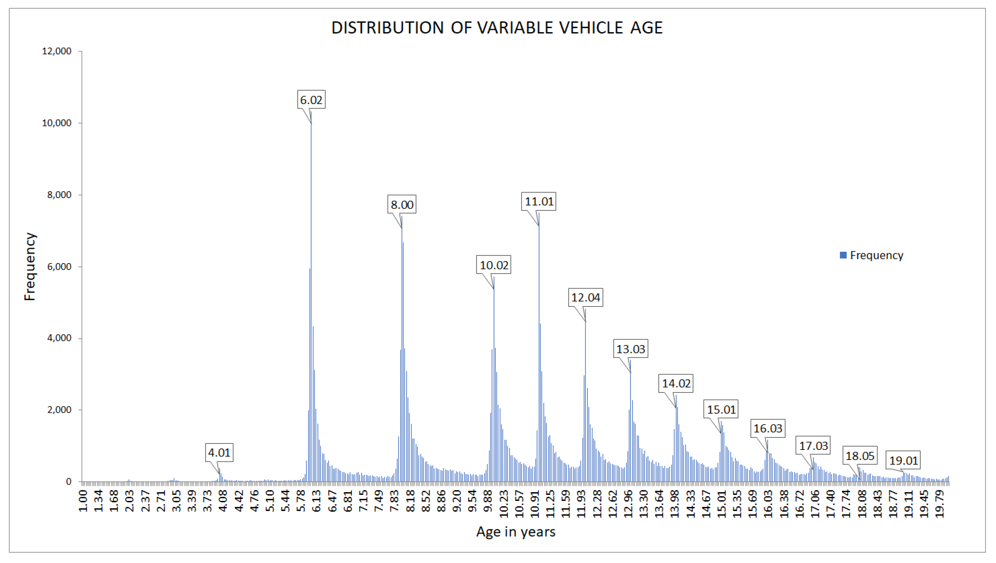
| Vehicle age | Vehicle age | 1 | 39.96 | 12.37 | 4.20 |
| Tare | Vehicle tare weight | 620 | 2960 | 1219 | 224.85 |
| Model | Hyperparameters Description | Value |
|---|---|---|
| CART | cp: Complexity parameter. | 0.01 |
| minsplit: The minimum number of observations that must exist in a node in order for a split to be attempted. | 5 | |
| maxdepth: Set the maximum depth of any node of the final tree, with the root node counted as depth 0. | 17 | |
| Random Forest | num.trees: Number of trees to grow. | 200 |
| mtry: Number of variables randomly sampled as candidates at each split. | 5 | |
| min.node.size: Minimal node size. | 10 | |
| sample.fraction: Fraction of observations to sample. | 0.5 | |
| Gradient Boosting | n.tress: Integer specifying the total number of trees to fit. | 1998 |
| Interaction.depth: Integer specifying the maximum depth of each tree. | 7 | |
| n.minobsinnode: Integer specifying the minimum number of observations in the terminal nodes of the trees. | 15 | |
| shrinkage: a shrinkage parameter applied to each tree in the expansion. | 0.1 | |
| bag.fraction: the fraction of the training set observations randomly selected to propose the next tree in the expansion. | 1 |
| Model | Training–Test Proportion | |||||||
|---|---|---|---|---|---|---|---|---|
| 80–20% | 70–30% | |||||||
| RMSE 1 | MAE 1 | R2 | MAPE | RMSE 1 | MAE 1 | R2 | MAPE | |
| CART | 1397.604 | 1146.963 | 0.670 | 0.084 | 1396.622 | 1147.038 | 0.669 | 0.084 |
| Random Forest | 1232.291 | 1042.873 | 0.744 | 0.076 | 1233.614 | 1043.207 | 0.742 | 0.076 |
| Gradient Boosting | 1220.328 | 1035.394 | 0.748 | 0.075 | 1221.665 | 1036.148 | 0.747 | 0.075 |
| Example 1 | Example 2 | Example 3 | Example 4 | Example 5 | Example 6 | |
|---|---|---|---|---|---|---|
| Vehicle age | 3 years | 4 years | 8 years | 8 years | 15 years | 15 years |
| Engine size | 2500 cm3 | 1600 cm3 | 2500 cm3 | 1600 cm3 | 2500 cm3 | 1600 cm3 |
| Tare | 1500 kg | 1000 kg | 1500 kg | 1000 kg | 1500 kg | 1000 kg |
| Age | 65 years | 40 years | 65 years | 40 years | 65 years | 40 years |
| Province | Madrid | Sevilla | Segovia | Valencia | Zaragoza | Barcelona |
| Seats | 5 | 4 | 5 | 4 | 5 | 4 |
| Lower bound 1 | 23,839 | 12,849 | 14,217 | 12,237 | 11,945 | 11,509 |
| RF prediction | 27,871 | 17,840 | 14,386 | 12,777 | 12,245 | 11,762 |
| GBM prediction | 25,008 | 17,384 | 14,415 | 14,084 | 12,210 | 11,499 |
| Upper bound 1 | 30,846 | 20,820 | 14,599 | 14,526 | 12,416 | 11,975 |
Publisher’s Note: MDPI stays neutral with regard to jurisdictional claims in published maps and institutional affiliations. |
© 2021 by the authors. Licensee MDPI, Basel, Switzerland. This article is an open access article distributed under the terms and conditions of the Creative Commons Attribution (CC BY) license (https://creativecommons.org/licenses/by/4.0/).
Share and Cite
Narváez-Villa, P.; Arenas-Ramírez, B.; Mira, J.; Aparicio-Izquierdo, F. Analysis and Prediction of Vehicle Kilometers Traveled: A Case Study in Spain. Int. J. Environ. Res. Public Health 2021, 18, 8327. https://0-doi-org.brum.beds.ac.uk/10.3390/ijerph18168327
Narváez-Villa P, Arenas-Ramírez B, Mira J, Aparicio-Izquierdo F. Analysis and Prediction of Vehicle Kilometers Traveled: A Case Study in Spain. International Journal of Environmental Research and Public Health. 2021; 18(16):8327. https://0-doi-org.brum.beds.ac.uk/10.3390/ijerph18168327
Chicago/Turabian StyleNarváez-Villa, Paúl, Blanca Arenas-Ramírez, José Mira, and Francisco Aparicio-Izquierdo. 2021. "Analysis and Prediction of Vehicle Kilometers Traveled: A Case Study in Spain" International Journal of Environmental Research and Public Health 18, no. 16: 8327. https://0-doi-org.brum.beds.ac.uk/10.3390/ijerph18168327