Article

Seasonal Variation, Chemical Composition, and PMF-Derived Sources Identification of Traffic-Related PM1, PM2.5, and PM2.5–10 in the Air Quality Management Region of Žilina, Slovakia

Department of Highway and Environmental Engineering, Faculty of Civil Engineering, University of Zilina, Univerzitná 8215/1, 010 26 Žilina, Slovakia
*
Author to whom correspondence should be addressed.
Int. J. Environ. Res. Public Health 2021, 18(19), 10191; https://0-doi-org.brum.beds.ac.uk/10.3390/ijerph181910191
Submission received: 6 August 2021 / Revised: 20 September 2021 / Accepted: 22 September 2021 / Published: 28 September 2021
(This article belongs to the Special Issue Advances in Airborne Pollution and Human Exposure Research)

Abstract

:
Particulate matter (PM) air pollution in the urban environment is mainly related to the presence of potential sources throughout the year. Road transport is one of the most important sources of PM in the urban environment, because it directly affects pedestrians. PM measurements were performed in the city of Žilina, Slovakia, at various road-traffic-related measurement stations over the course of several years. This paper evaluates changes in the concentration of the fine fraction (PM2.5), the ultrafine fraction (PM1), and the coarse fraction (PM2.5–10) over time. PM concentrations were measured by reference gravimetric method. Significant changes in PM concentrations over time due to the diversification of pollution sources and other, secondary factors can be observed from the analysis of the measured data. PM samples were subjected to chemical analysis inductively coupled plasma mass spectrometry (ICP-MS) to determine the concentrations of elements (Mg, Al, Ca, Cr, Cu, Fe, Cd, Sb, Ba, Pb, Ni, and Zn). The seasonal variation of elements was evaluated, and the sources of PM2.5, PM1, and PM2.5–10 were estimated using principal component analysis (PCA) and positive matrix factorization (PMF). PM2.5 (maximum concentration of 148.95 µg/m3 over 24 h) and PM1 (maximum concentration of 110.51 µg/m3 over 24 h) showed the highest concentrations during the heating season, together with the elements Cd, Pb, and Zn, which showed a significant presence in these fractions. On the other hand, PM2.5–10 (maximum concentration of 38.17 µg/m3 over 24 h) was significantly related to the elements Cu, Sb, Ba, Ca, Cr, Fe, Mg, and Al. High correlation coefficients (r ≥ 0.8) were found for the elements Mg, Ca, Fe, Al, Cd, Pb, and Zn in the PM1 fraction, Cd, Pb, and Zn in PM2.5, and Ba, Sb, Fe, Cu, Cr, Mg, Al, and Ca in PM2.5–10. Using PMF analysis, three major sources of PM (abrasion from tires and brakes, road dust resuspension/winter salting, and combustion processes) were identified for the PM2.5 and PM1 fractions, as well as for the coarse PM2.5–10 fraction. This study reveals the importance of non-exhaust PM emissions in the urban environment.

1. Introduction

PM is a common proxy indicator of air pollution. The main components of PM are sulfates, nitrates, ammonia, sodium chloride, black carbon, mineral dust, and water. It consists of a complex mixture of solid and liquid particles of organic and inorganic substances suspended in air. While particles with a diameter of 10 micrometers or less (≤PM10) can penetrate and settle deep inside the lungs, particles with a diameter of 2.5 micrometers or less (≤PM2.5) are even more harmful, as they can penetrate the pulmonary barrier and enter the bloodstream [1].
Epidemiological studies have shown that exposure to PM emissions—in particular PM2.5—is associated with various short-term and long-term adverse health effects, such as increased risks of cardiovascular, respiratory, and developmental conditions, as well as an increased risk of overall mortality [2,3,4]. Oxidative stress caused by metals and organic compounds found in PM emissions is considered to be the main biological mechanism responsible for these adverse health effects. Recent research also suggests that air pollution exacerbates epidemics of coronaviruses such as SARS and COVID-19. Such impacts are greatest in urban areas, where emission levels are highest [5,6,7,8,9,10,11,12].
The concentrations, composition, and nature of air pollutants depend mainly on the period and place that are monitored and evaluated for air quality management purposes. In terms of temporality, the dynamics of such processes can be divided into three basic levels: long-term trends, annual course (seasonal changes), and daily course. In terms of the nature of the locality wherein the air quality is monitored, pollutants are commonly divided into urban, rural, and background pollutants.
The annual course (seasonal changes) usually expresses the interaction between specific human activities (use of a certain type of resource) and meteorological conditions that accompany or determine the nature of pollution (temperature, wind, sunshine, etc.). A typical example is the increase in SO2, NOx, and aerosol concentrations in winter, when increased concentrations of pollutants are caused not only by higher emissions (more sources in winter), but also by low temperatures and inversions, which facilitate the formation, persistence, and slow deposition of pollutants (meteorological parameters). Seasonal changes in PM concentrations may indicate the presence of different sources of air pollution in a particular area [13,14,15,16,17,18,19,20,21].
The main sources of PM air pollution in urban areas include road transport and domestic heating with wood and coal [14,15,22,23,24,25,26,27,28,29,30]. Emissions of PM from motor vehicles originate from two main sources: the combustion of fossil fuels—whose emissions are released via tailpipe exhaust [25,28,31,32]—and non-exhaust processes, including the degradation of vehicle parts and road surfaces [25,33,34,35,36,37,38,39], as well as the resuspension of road dust. The airborne particulate emissions generated by these processes are defined as non-exhaust PM emissions [25,28,34,38,40,41]. PM emissions from road transport directly affect pedestrians in urban areas, with their concentrations often exceeding safe limits for human health [42,43]. The weight, number, size, and chemistry of the particles affect the toxicity of the PM [44,45,46,47,48,49,50,51].
Non-exhaust emissions of PM are beginning to play a major role in the environment, as exhaust emissions of PM have been successfully reduced by introducing direct measures on vehicles (Table 1) [40].
Regarding the chemical composition of PM [2,18,25,45,49,54,55], evidence is still accumulating on the adverse effects of oxidative stress—which is often associated with transition metals and redox-active organic substances such as quinone—on human health [56,57,58,59]. Vehicle-derived particles have a high oxidation potential [59], and a clear increase in the oxidation potential of PM on the road has been found to be associated with metals from non-exhaust emissions [25,32,40,60] (Table 1). Increases in the oxidative potential of such particles are significant, and the metal components identified as determinants of this oxidative activity are toxic to humans [61]. These results are important because they highlight the contribution of currently unregulated pollutants from non-exhaust emissions to negative health outcomes.
The presence of aluminum and silicon in PM has been associated with health problems—especially respiratory problems [62,63,64]. Other elements—including iron, copper, zinc, and sulfur—have also been shown to be associated with adverse health effects, such as cardiopulmonary oxidative stress, heart rate variability, and tissue damage in vivo [65,66,67]. For example, tests on laboratory animals have shown that combined exposure to tire dust, zinc, and copper in high concentrations can lead to oxidative stress in the heart [68].
The present study focuses on the analysis of data on air pollution by PM in the city of Žilina, Slovakia. PM is the most critical pollutant in the city of Žilina, and it is desirable to study its origin as well as any changes in its composition. The aim of this study was to reveal seasonal changes in PM concentrations and to establish the source structure of this pollutant.
The city of Žilina has long been included on the list of air quality management areas in Slovakia. Air quality management areas are already recognized as an area with poor air quality identified by using monitoring stations at which measures to improve air quality need to be prioritized. This is mainly based on the exceeding of the safe limits of concentrations of PM10 and PM2.5 for the protection of public health [69]. Therefore, these measurements were focused on the sampling of three fractions of PM (PM10, PM2.5, and PM1). The measurements were performed at seven different traffic-related urban measuring stations during different years and seasons. The measured values provide us with a picture of changes in PM concentrations over the course of the year, during which various sources of pollution are present in the air quality management area (the city of Žilina). The retrospective identification of sources of PM—based on knowledge of their chemical composition, and the possible origin of individual elements—can be an effective tool in the process of eliminating air pollution in cities. PM was chemically analyzed using ICP-MS to determine the presence of selected metals (Mg, Al, Ca, Cr, Cu, Fe, Cd, Sb, Ba, Pb, Ni, and Zn). These elements can come from a variety of sources. Using multidimensional statistical methods and knowledge of the origins of these elements, the sources of PM were estimated. Some of the methods that can be used for this process include principal component analysis (PCA), factor analysis (FA) [70,71,72,73,74,75,76], and positive matrix factorization (PMF) [76,77,78,79,80]. In some previous studies, we focused on identifying PM10 sources using PCA and FA [55,81]. In this study, we focused on the PM1, PM2.5, and PM2.5–10 fractions. The PCA and PMF methods were selected for this study. Using the PCA method, the minimum number of hidden variables is determined along with the maximum number of original data; thus, the dimensionality of the solution is reduced. A number of relevant factors for use in PMF were identified using PCA. Using PMF, elements were divided into factors (sources of PM emissions), and their scores were determined, which were then regressed against concentrations in order to estimate the relative contribution of each source. This study focuses on elucidating the composition of PM sources at traffic-related measuring stations, focusing on the negative potential of the formation of non-exhaust PM emissions, and their overall contribution to PM.

2. Materials and Methods
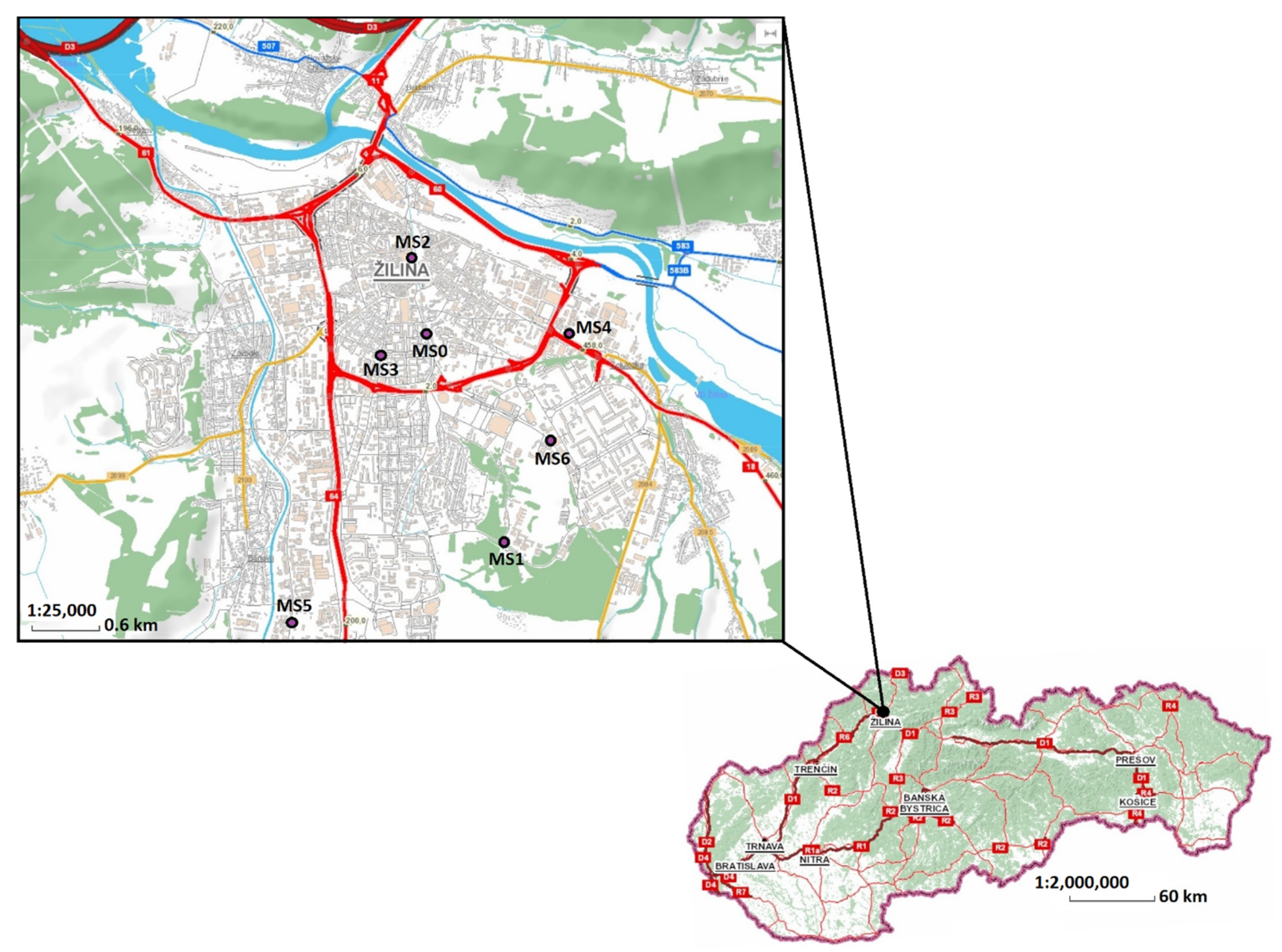
2.1. Study Area

Particulate measurements were performed in the air quality management region in the city of Žilina, Slovakia (Figure 1). Measurements were performed from 2010 to 2019 at different measuring stations—especially near roads—during different measuring periods (Table 2).
A total of 99 PM samples each were taken from the PM10, PM2.5, and PM1 fractions using a nitrocellulose filter, following the gravimetric method. The particulate samples were then subjected to chemical analysis.

2.2. Measurements of PM

To establish the amount of ambient PM present in the air, a reference method (the gravimetric method) was applied, pursuant to the STN EN 12341 standard (2016). The sampling was performed using three low-volume flow samplers (LECKEL LVS3 Low-Volume Samplers, Sven Leckel Ingenieurbüro GmbH). Three fractions of PM were monitored concurrently—specifically, PM10, PM2.5, and PM1. The PM was collected on the nitrocellulose filters for 24 h (10 a.m.–10 a.m. the next day). Finally, using this method, we obtained seven 24 h concentrations for each PM fraction at each measurement station (99 filters for each PM fraction—in sum, 297 exposed filters). The nitrocellulose filters had a diameter of 47 mm, and the PM was collected at a fixed airflow rate of 2.3 m3/h, after which the mass of PM collected on the filters was determined by means of microbalances, calculated on the basis of the known volume of air obtained during sampling (µg/m3). The PM2.5–10 concentration was determined as the difference between the fractions PM10 and PM2.5. All the contamination filters (samples of PM) were used for elemental chemical analysis.
QA/QC: All necessary steps were taken to ensure the quality of the samples and the PM concentrations, including checkweighing. We calibrated all of the measuring instruments as prescribed by the STN EN 12341 standard, and quantified the total uncertainty of the method for PM1, PM2.5, and PM10, consisting of partial uncertainties—sampling of PM by a flow pump and weighing of clean and exposed nitrocellulose filters. This method is maintained as an accredited method at our workplace.

2.3. Chemical Analysis of PM

The collected PM contained various elements and compounds. In the next phase of the research, chemical analyses of PM10, PM2.5, and PM1 were performed. Particulate matter was captured on cellulose nitrate (CN) membrane filters. We focused on monitoring 12 elements, which we selected based on their likely origin (source) (Mg, Al, Ca, Cr, Cu, Fe, Cd, Sb, Ba, Pb, Ni, and Zn). Each of these elements comes from a specific source [22,24,25,28,34,54,55,82]. The concentrations of the elements were determined in each sample of PM10, PM2.5, and PM1. The concentrations of elements in the PM2.5–10 were determined as the difference between the concentrations of the element in the PM10 and PM2.5 fractions.
To identify and determine the concentrations of elements in the PM samples, spectroscopic methods were utilized (inductively coupled plasma mass spectrometry (ICP-MS)). The analyses of the 297 filters (99 filters for each PM fraction) and the determination of elements present in the PM10, PM2.5, and PM1 fractions were performed in accordance with the STN EN 14902 standard (2006).
The filters were digested in Teflon vessels with nitric acid (HNO3) at a temperature of 230 °C, using a high-temperature and high-pressure SW-4 microwave digestion system (Berghof, Germany). Samples were transferred and appropriately diluted before element determinations on a triple-quadrupole ICPMS (Agilent 8800 Triple-Quadrupole ICP-MS, Japan). The tests were carried out in the laboratory of the Transport Research Centre in Brno, Czech Republic. The final concentration of each element (ng/m3) was determined as the difference between the detected concentration of the element in the sample (decomposed exposed filter) and the concentration of the element in the blank (decomposed clean filter).
QA/QC: Chemical analyses were performed using the accredited ICP-MS method within the Transport Research Center in Brno, Czech Republic. Appropriate certified reference materials (CRMs) as calibration standards were used to determine the concentrations of these chemical elements. Measurement uncertainties were determined for individual elements, and were subsequently used in PMF analysis as inputs to the calculations. The QA/QC of this method is an exclusive part of the institution’s accredited laboratory.

2.4. Data Analysis

The concentrations of PM10, PM2.5–10, PM2.5, and PM1, along with the various tested elements, were subjected to various mathematical analyses. Data matrices measuring 13 variables × 99 measurements were constructed, which contained the concentrations of both the elements and the respective PM fraction.
An important factor in air quality monitoring is the time variation of pollutants. For the purposes of this study, we observed the time variation of PM and the elements that it contains. For this purpose, we used the computer programming language R with the open-air air pollution analysis package [83,84].
R is a computer programming language developed specifically for the purposes of analyzing data (R-project). It is variously described as a statistical system, a system for statistical computation and graphics, and an environment for data analysis and statistics.
The timeVariation function produces four plots: day of the week variation, mean hour of the day variation, a combined hour of the day/day of the week plot, and a monthly plot. We mainly used a monthly plot in order to determine the annual course of concentrations of PM and its constituent elements (Figure 2 and Figure 3). The plots also show the 95% confidence interval of the mean. These uncertainty limits can be helpful when trying to determine whether one candidate source is different from another. The uncertainty intervals were calculated through bootstrap re-sampling, which provides better estimates than the application of assumptions based on normality—especially when there are few data available. The function can consider one or more input variables. It should also be noted that variables other than pollutant concentrations can be considered, e.g., meteorological data. The timeVariation function is probably one of the most useful functions for the analysis of air pollution.
Furthermore, correlation analysis was used, where the relationship between individual elements was identified (Figure 4, Figure 5 and Figure 6).
We also used Pearson’s correlation (r), which measures a linear dependence between two variables (x and y). This is also known as a parametric correlation test, because it depends on the distribution of the data. It can be used only when x and y are normally distributed. The plot of y = f(x) is known as the linear regression curve.
r = ( x m x ) ( y m y ) ( x m x ) 2 ( y m y ) 2
where:
  • x and y are two vectors of length n;
  • mx and my correspond to the means of x and y, respectively.
The p-value (significance level) of the correlation can be determined by using the correlation coefficient table for the degrees of freedom: df = n − 2, where n is the number of observations in the x and y variables, or by calculating the t value as follows:
t = r 1 r 2 n 2
where the corresponding p value is determined using the t distribution table for df = n − 2. If the p value is <0.05, then the correlation between x and y is significant.
The correlation coefficient ranges between −1 and 1:
  • −1 indicates a strong negative correlation: this means that every time x increases, y decreases;
  • 0 means that there is no association between the two variables (x and y);
  • 1 indicates a strong positive correlation: this means that y increases with x;
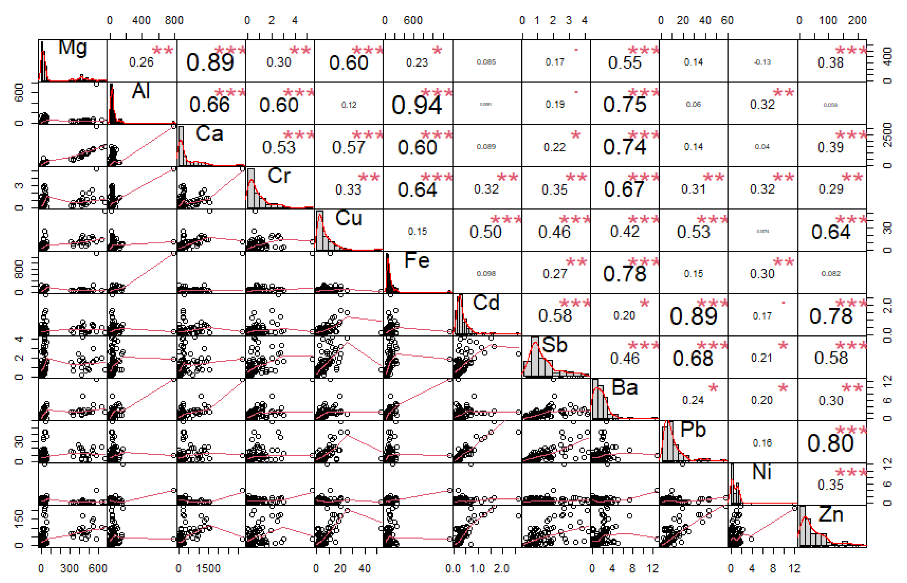
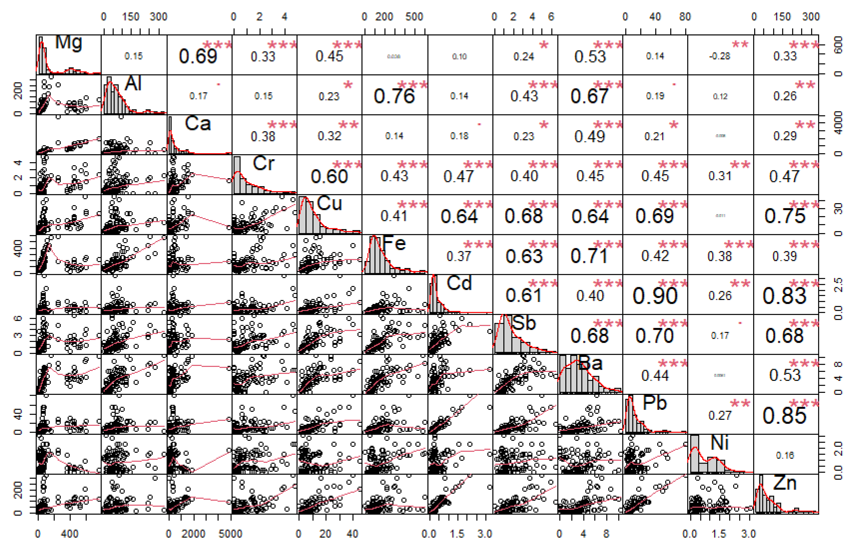
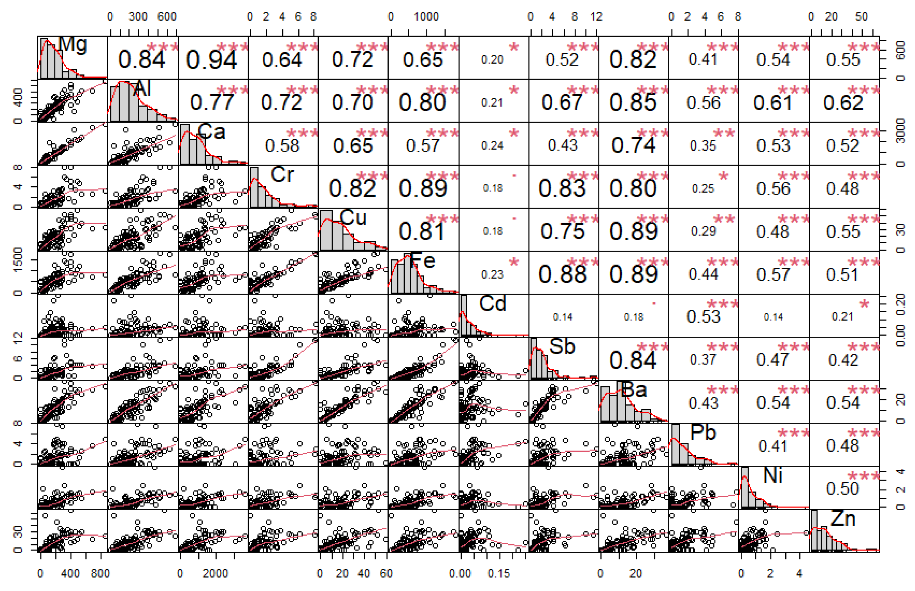
  • The function chart.Correlation() in the package PerformanceAnalytics in R can be used to display a chart of a correlation matrix;
  • The output of the correlation analysis performed in R is shown in Figure 4, Figure 5 and Figure 6, which contain the following information:
  • The distribution of each variable is shown on the diagonal;
  • At the bottom of the diagonal, the bivariate scatter plots are displayed with a fitted line;
  • At the top of the diagonal, the value of the correlation plus the significance level are shown as stars;
  • Each significance level is associated with a symbol: p-values (0, 0.001, 0.01, 0.05, 0.1, 1) <=> symbols (“***”, “**”, “*”, “.”, “ “)
In the next phase of data analysis, two methods of multidimensional statistical analysis were used—PCA and PMF [55,76,77,78,85]. These methods lead to a reduction in the size of the original task, i.e., transformation of the original variables (elements) into a smaller number of latent variables, so as to preserve as much information as possible about the original data. The results illustrate the interconnection of some elements in the data matrix, along with the subsequent interpretation of their structure based on individual factors—namely, the source of the PM.
The primary goal of PCA is the transformation of the original characters of xj, j = 1, …, m into a smaller number of latent variables yj. These latent variables possess more appropriate and comprehensive properties: their presence is less significant, they capture and represent almost the entire variability of the original characteristics, and their properties are mutually uncorrelated. Latent variables are regarded as the main components, and they represent linear combinations of former variables. The first principal component (PC) y1 describes the greatest part of the variability and, hence, the distribution of the original data, the second principal component y2, on the other hand, describes the second-greatest part of the variability, capturing the distribution not accounted for within y1, etc. (Figure 7). Mathematically speaking, the first PC is viewed as a linear combination of input characters that covers the greatest variability, spread between the other linear combinations. In the matrix form, we establish the PCA model of the following string [55,70,72,75,78,85,86]:
X = T P T + E
where:
  • X: source matrix;
  • T: matrix of the component score;
  • PT: transposed matrix of the component loadings; and
  • E: matrix of residues,
and for the first PC, the following relation prevails:
y 1 = j = 1 m v 1 j x j
where:
  • xj: former character, input variable, j = 1, …, m;
  • v1j: coefficients of eigenvectors.
Receptor models are mathematical approaches to quantifying the contribution of sources to samples based on the composition or fingerprints of the sources. The composition or speciation is determined using analytical methods appropriate for the medium, and key species or combinations of species are needed to separate impacts. A speciated dataset can be viewed as a data matrix X of i by j dimensions, in which i samples and j chemical species are measured, with u uncertainties. The goal of receptor models is to solve the chemical mass balance (CMB) between measured species concentrations and source profiles, as shown in Equation (5), with the number of factors p, the species profile f of each source, and the amount of mass g contributed by each factor to each individual sample [23,55,70,71,72,74,85,86]:
x i j = k = 1 p g i k f k j + e i j
where eij is the residual for each sample/species.
To establish the appropriateness of the factor analysis adopted here, the KMO (interval 0–1) and MSA (interval 0–1) criteria were calculated. In accordance with these criteria, the adoption of factor analysis was substantiated.
The CMB equation can be solved using multiple models, including EPA CMB, EPA Unmix, and EPA Positive Matrix Factorization (PMF). PMF is a multivariate factor analysis tool that decomposes a matrix of speciated sample data into two matrices: factor contributions (G), and factor profiles (F). These factor profiles need to be interpreted by the user in order to identify the source types that may be contributing to the sample, using measured source profile information and emission or discharge inventories. The method is briefly reviewed here, and described in greater detail elsewhere [76,77,78,79,80]. Results are obtained under the constraint that no sample can have significantly negative source contributions. PMF uses both sample concentration and user-provided uncertainty associated with the sample data to weigh individual data points. This feature allows analysts to account for the confidence in the measurement. For example, data below detection limits can be retained for use in the model, with the associated uncertainty adjusted so that these data points have less influence on the solution than measurements above the detection limit. Factor contributions and profiles are derived by the PMF model minimizing the objective function Q:
Q = i = 1 n j = 1 m [ x i j k = 1 p g i k × f k j u i j ] 2

3. Results

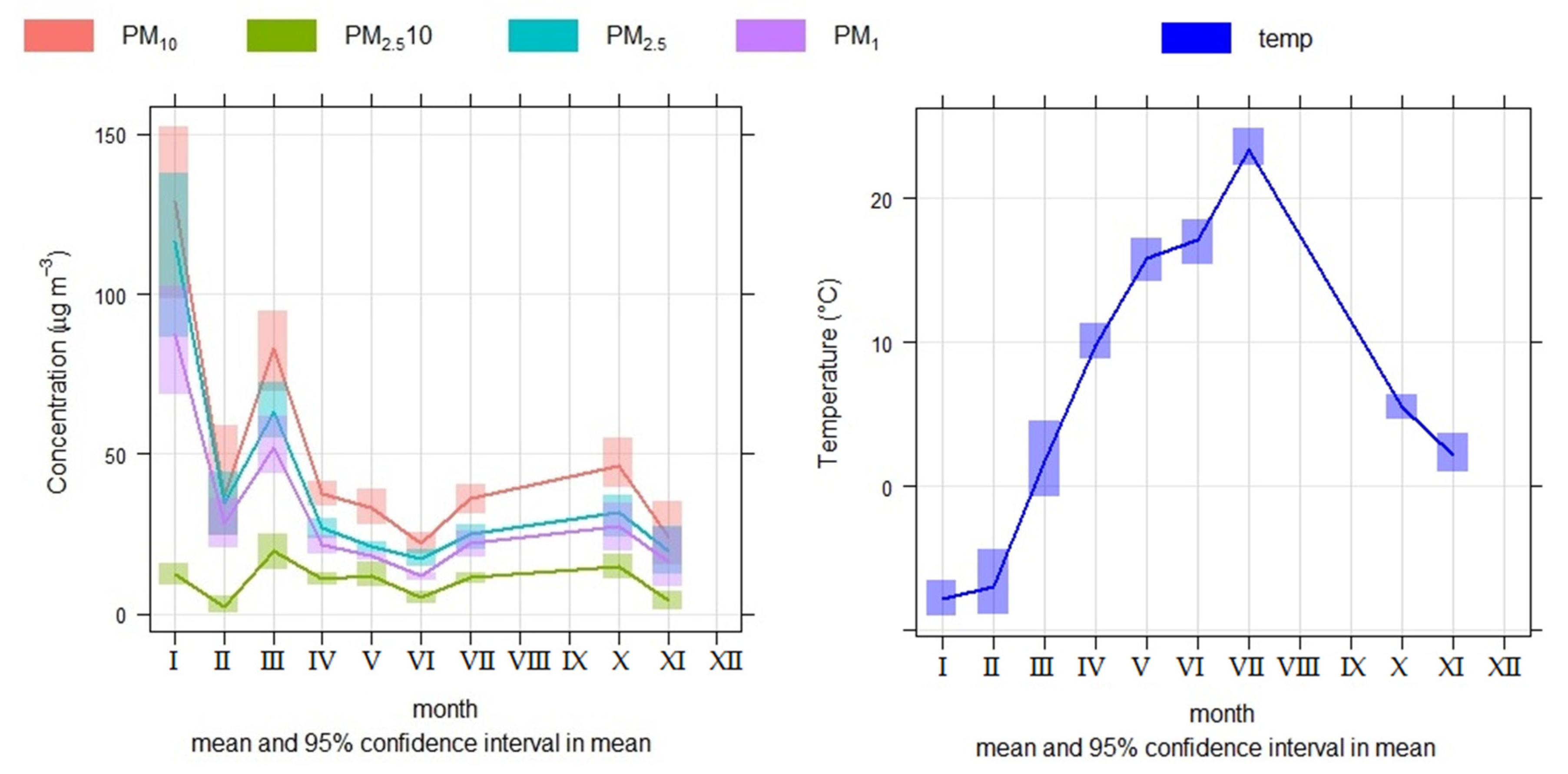
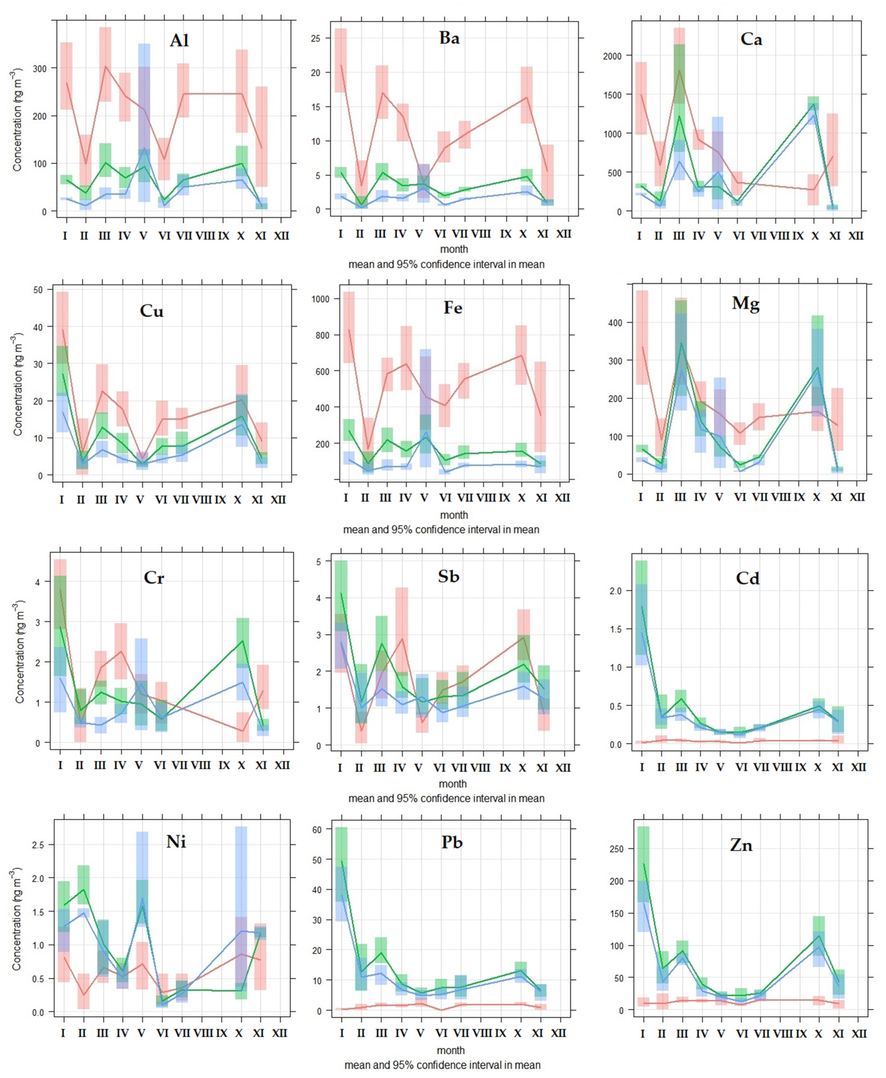
3.1. Time Variation Analysis

The analysis of time variation was used to investigate seasonal changes in PM concentrations—especially the PM2.5, PM1, and PM2.5–10 fractions. The analysis showed that the concentrations of PM2.5 and PM1 tend to be significantly higher in periods with low temperatures (Figure 2). The significance of the effect of temperature on PM2.5 and PM1 concentrations was subjected to correlation analysis. The correlation coefficients produced the following values: for PM2.5 vs. temperature, r = −0.54; and for PM1 vs. temperature, r = −0.52. Correlations were significant at the level of p < 0.05. The high concentrations in the cold season were mainly due to the presence of seasonal sources, such as local heating, along with suitable conditions for the formation of secondary particles in the air [87]. On the other hand, the PM2.5–10 fraction shows an even distribution throughout the year (Figure 2). Road transport contributes greatly to this fraction—especially non-exhaust PM emissions and road dust resuspension [22,25,27,28,38,40,41,45,54,88,89,90,91]; the value found in this study was a contribution of 76.7%. This PM fraction is affected evenly throughout the year by road traffic volume, as well as meteorological factors such as wind speed and rainfall [92]. These factors generate changes in PM concentrations via dry or wet deposition.
The statistical evaluation of all measured concentrations of PM during the mentioned periods is shown in Table 3. The maximum concentration of PM2.5 was measured on 29 January 2012 (148.95 µg/m3), at which time the concentration of PM1 was 110.51 µg/m3.
The concentrations of elements in PM are also subject to seasonal changes. We evaluated changes in the concentrations of elements in PM2.5, PM1, and PM2.5–10. The intention was to distinguish between groups of elements that may predominate in the PM2.5 and PM2.5–10, and vice versa. Elements that predominate in the PM2.5–10 (Al, Ba, Ca, Cu, Fe, and Mg) can be formed by mechanical wear from permanent sources over the course of the year, such as from road transport, e.g., non-exhaust emissions and road dust (year-round sources) [25,28,34,40]. On the other hand, there are also elements that predominate in the PM2.5 (Cd, Ni, Pb, and Zn), whose concentrations increase significantly (>100%) during the heating season (Table 4). Here, the influence of a seasonal source of PM is assumed—local heating [26,31,73,76,82]. If we use the criterion of the beginning of the heating season in Slovakia, when the average daily temperature is <13 °C (Act on Thermal Energy No. 657/2004 Coll. and Decree of the Ministry of Economy of the Slovak Republic No. 152/2005 Coll., on the specified time and on the specified quality heat supply for the final consumer, respectively), we found an increase in the average concentrations of PM2.5 and PM1 of 81.4% and 76.2%, respectively, compared to the average concentrations during the non-heating season (average daily temperature > 13 °C). On the other hand, PM2.5–10 does not show such a change (Figure 2).
The average concentrations of Mg, Ca, and Cd increased during the heating season in PM2.5–10, while Mg, Ca, Cr, Cu, Cd, Sb, and Pb concentrations increased in PM2.5 and PM1 (Table 4; Figure 3). The greatest change can be observed for Mg and Ca in the PM2.5 fraction (Table 4). The average concentrations of Mg (174.94 ng/m3) and Ca (555.14 ng/m3) in the PM2.5 fraction were calculated by comparing the values obtained at temperatures < 13 °C to the average concentrations of Mg (57.45 ng/m3) and Ca (249.83 ng/m3) obtained at temperatures > 13 °C. This phenomenon is related to winter road maintenance, which ensures the mitigation of defects in the passibility and stairness of roads caused by winter weather conditions. Compounds such as sodium chloride, calcium chloride, magnesium chloride, and others are used as defrosting agents. The purpose of the use of magnesium chloride-based spreading materials on roads is to eliminate faults in the passibility of roads, as a step in their winter maintenance, so as to help road managers to maintain the roads’ normal condition. This helps to increase safety on roads in winter, as well as assisting with troubleshooting of roadworthiness, and providing an outlet for the ecological disposal of magnesium chloride. However, elements contained in spreading materials enter the air, water, and soil, affecting their natural state [93].
An increase in concentration during the heating season is also observed for the elements Cd, Pb, and Zn—mainly in the PM2.5 fraction; this change is probably related to local heating and combustion processes [30,76,78]. On the other hand, we can also observe a decrease in the concentrations of some chemical elements during the heating season, which is reflected mainly in the PM2.5–10 fraction for the elements Al, Cr, Cu, Fe, Sb, Ba, Pb, Ni, and Zn (Table 4, Figure 3). Some of these elements represented in the PM2.5–10 fraction are related to road transport—specifically, to non-exhaust emissions of PM [22,25,34,39,40]. The primary source of PM in the city of Žilina is road transport during the non-heating season—mainly non-exhaust PM emissions (e.g., road surface abrasion, tires, brakes, and road dust resuspension), which, under the more suitable dispersion conditions during the non-heating season, can enter the ambient air more easily and can stay there for some time. This claim is also supported by subsequent analyses of PCA and PMF.

3.2. Elemental Correlation Analysis

The performed correlation analysis of the concentrations of elements in individual fractions of PM revealed some internal bonds between the variables. The elements Mg/Ca, Fe/Al, and Cd/Pb/Zn in the PM1 fraction show high correlation coefficients (r ≥ 0.8) (Figure 4). In the PM2.5 fraction, the elements Cd/Pb/Zn show high correlation coefficients (Figure 5). Significant correlations between Ba, Sb, Fe, Cu, Cr, Mg, Al, and Ca were found in the PM2.5–10 (Figure 6). Non-exhaust emissions of PM (e.g., road surface abrasion, tire abrasion, brake and clutch wear) were primarily responsible for the formation of the PM2.5–10 [25,28,34,39]. This is further supported by significant correlations between elements, which may indicate a common source of PM [25,28,31,34,40].

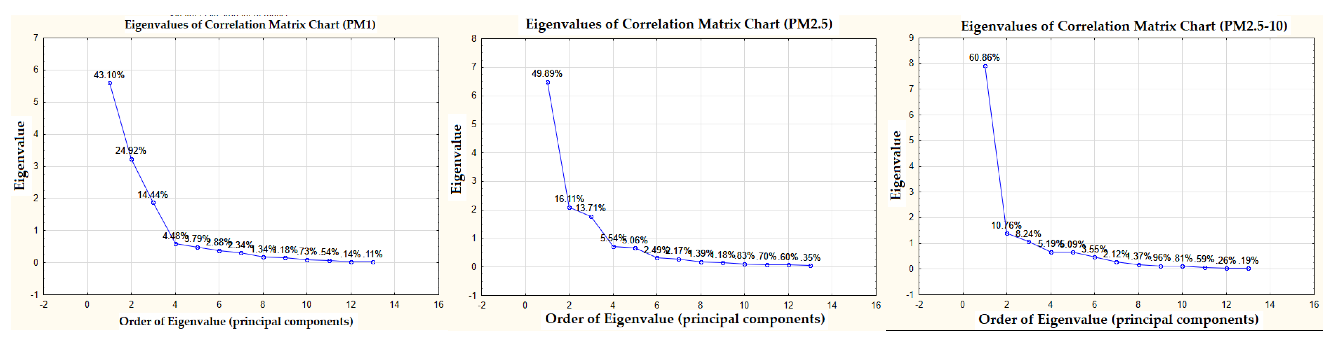
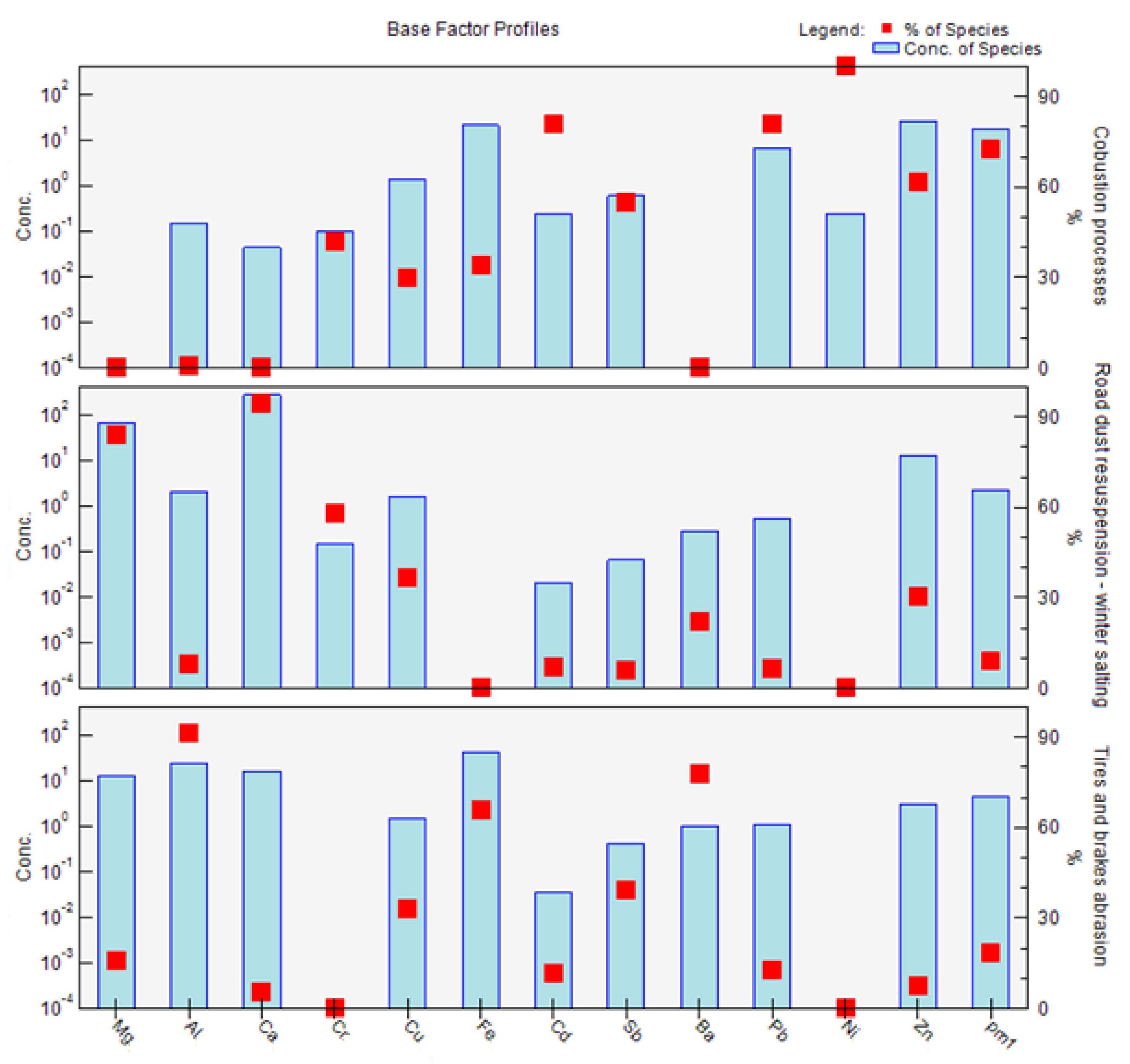
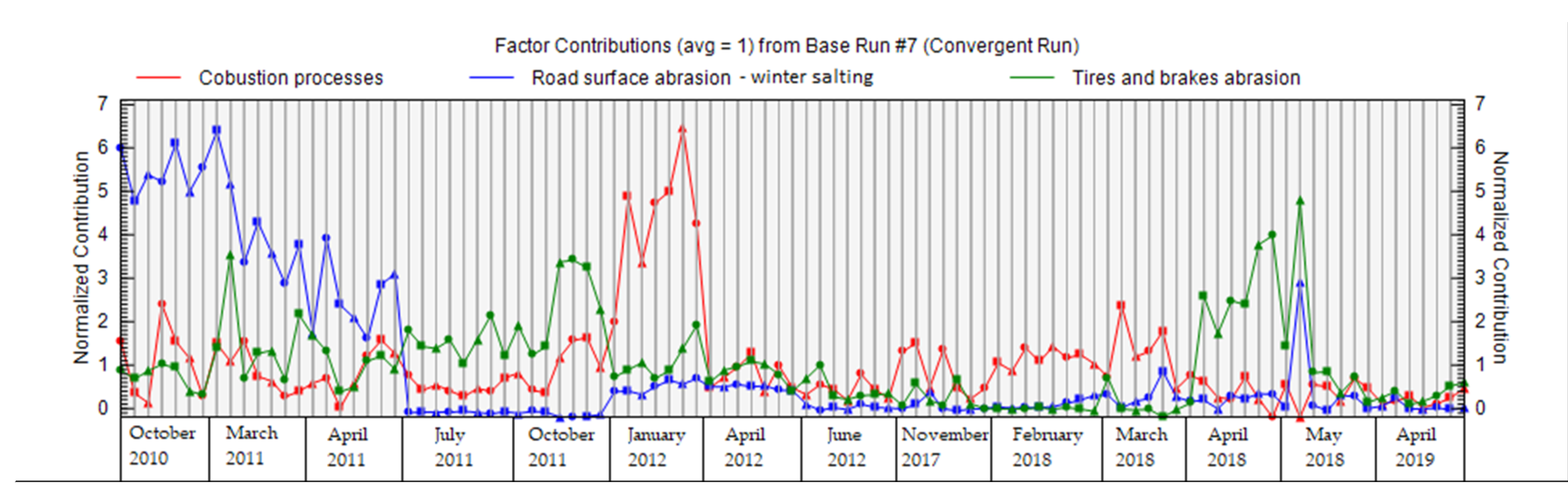
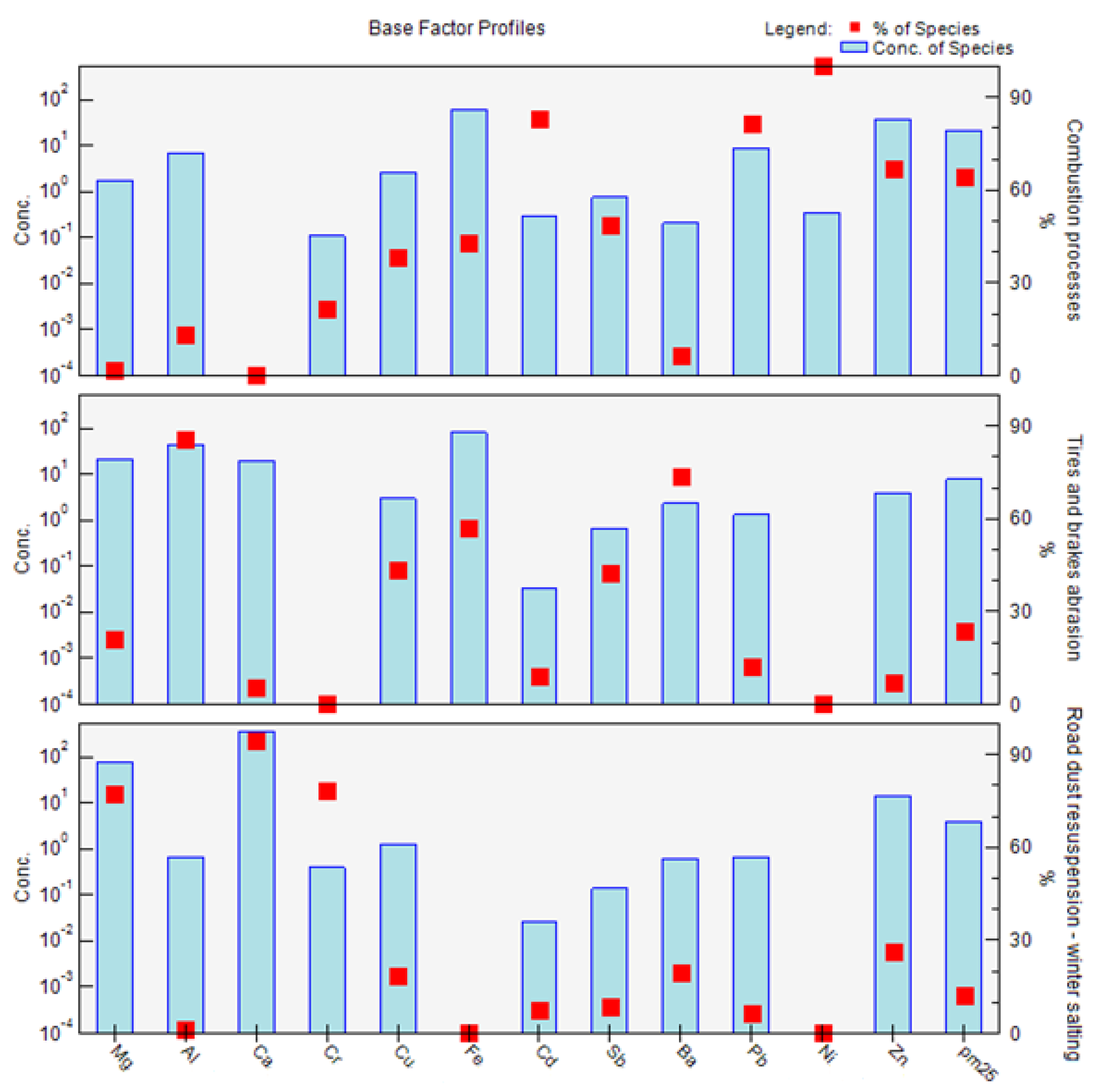
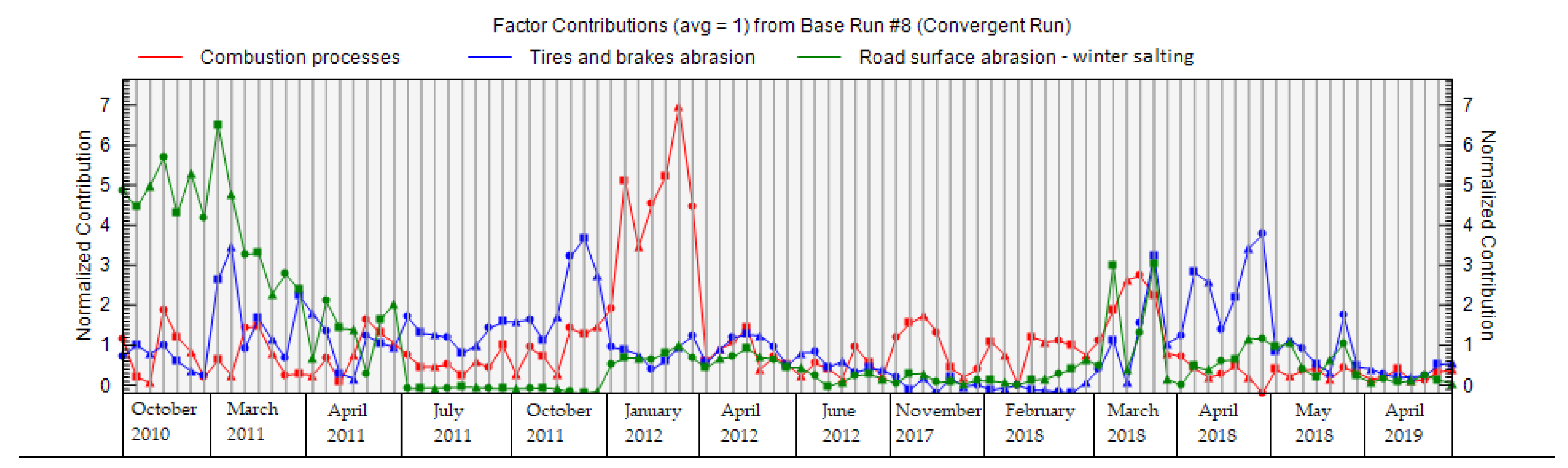
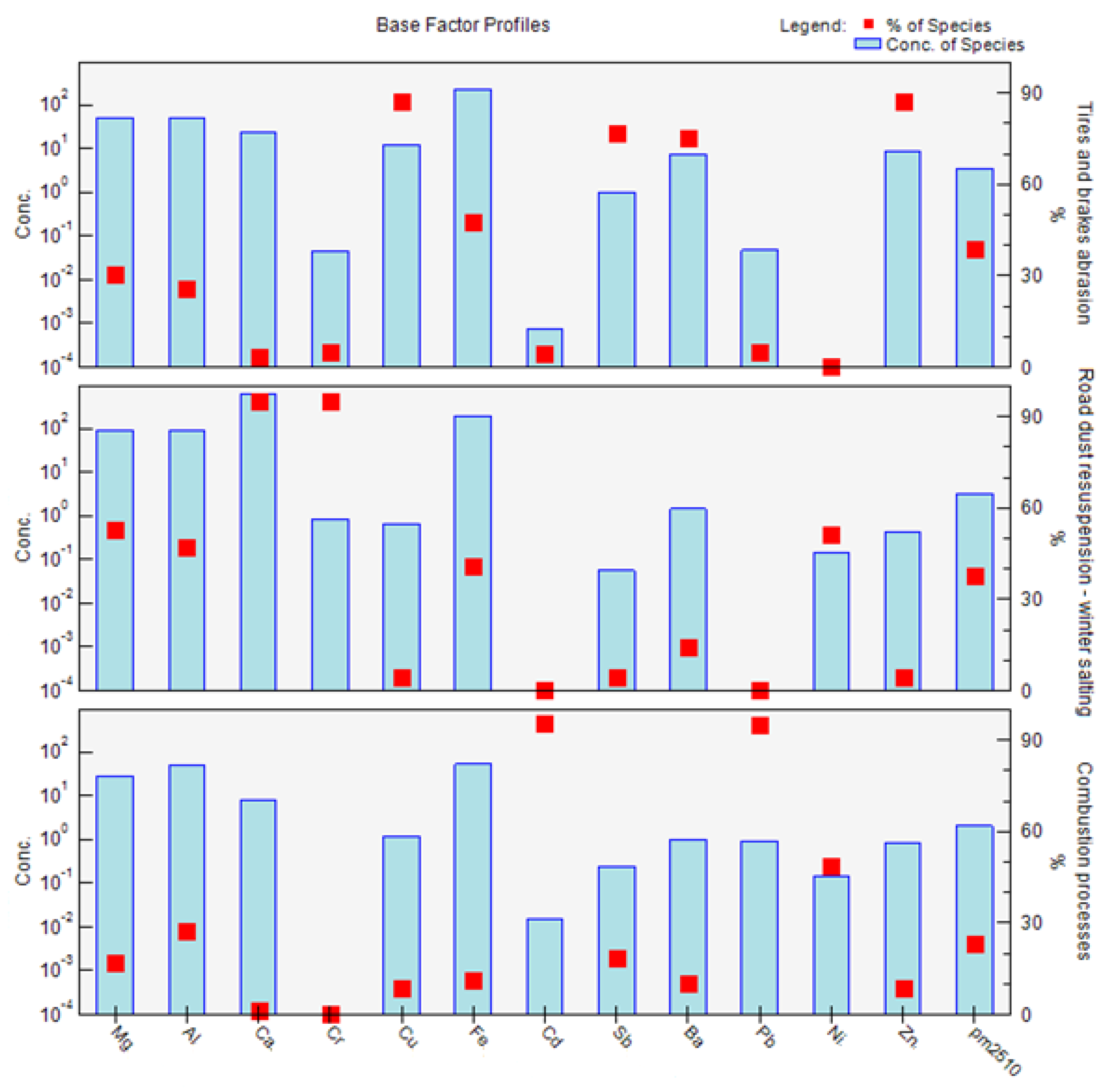
3.3. PCA and PMF Analyses

Furthermore, PMF (EPA PMF 5.0 program [77]) was used to explain the internal bonds between elements in PM. An uncertainty dataset that assigns an uncertainty value to each species was also used. Uncertainties determined for individual elements using the ICP-MS method, along with uncertainties determined for PM using the gravimetric method, were used for the calculation. The result of the analysis was the identification of various sources of PM1, PM2.5, and PM2.510.
Using PCA, three main components were extracted for the PM1, PM2.5, and PM2.5–10 fractions, each of which reached an eigenvalue > 1. In the case of PM1, these three principal components characterized 82.5% of the variance of the original data; in the case of PM2.5, they characterized 79.7%; and in the case of PM2.5–10, they characterized 79.9% (Figure 7). Subsequently, these three principal components were used in the PMF analysis for all of the PM fractions.
The bootstrap (BS), displacement (DISP), and BS-DISP error estimation were used for every PM model:
  • DISP results show that the solution is stable because no swaps are present;
  • BS results—mapping over 80% of the factors indicates that the BS uncertainties can be interpreted and the number of factors may be appropriate;
  • BS-DISP results—the number of swaps is one for two factors, which indicates some ambiguity between the factors. The number of swaps is low.
On the basis of the results of the criteria, factor analysis can be applied for PM1 (KMO = 0.7, reflecting average correlation between the variables; MSA > 0.5, indicating that the i-th variable is at least moderately predicted by the others), for PM2.5 (KMO = 0.8, reflecting good correlation between the variables; MSA > 0.6, indicating that the i-th variable is at least moderately predicted by the others) and for PM2.5–10 (KMO = 0.8, reflecting good correlation between the variables; MSA > 0.6, indicating that the i-th variable is at least moderately predicted by the others).
The factor composition obtained via PMF analysis for the PM1 fraction is shown in Figure 8. The profile graph for the PM1 fraction (Figure 8) shows the concentration of each species (element) assigned to the factor as a pale blue bar, and the percentage of each species assigned to the factor as a red box. The concentration line corresponds to the left y-axis, which is a logarithmic scale; the percentage of species corresponds to the right y-axis. Factor 1 is therefore characterized mainly by the elements Cd, Pb, Ni, and Zn if we take into account the classification criterion > 60%. In the case of factor 2, the major elements are Mg, Ca, and Cr. Factor 3 is characterized by the elements Al, Fe, and Ba. The factors are characterized according to the representation of individual elements in their profiles according to the possible source of the combination of elements, the time distribution of PM and elemental concentrations over the course of the year, and the interrelationships between the elements (correlations) (Figure 8).
Figure 9 shows the contribution of all factors to the total weight of the sample; this graph can be used to verify the names of factors, and to determine the distribution of factors for individual species (elements). The largest contribution of factor 1 was combustion processes in January 2012, during the heating season. This period was characterized by very low temperatures and considerable inversion, indicative of a significant heating season. The main contribution of factor 2—road dust resuspension and winter salting—to PM1 concentrations was most pronounced in the periods of October 2010, March 2011, and April 2011, when spreading materials were widely used to ensure road safety; these periods were characterized by low temperatures and frequent icing on the roads. The main contribution of factor 3—abrasion of tires and brakes—does not show such extremes as factors 1 and 2, and is mostly uniform across different measurement periods (Figure 9).
Factors 1–3 contribute to the PM1 variable as follows—factor 1: 72.4%; factor 2: 9.1%; factor 3: 18.4%—according to the PMF results. It is clear that combustion processes make a significant contribution to the formation of PM1. The contributions of individual factors are characteristic of the periods and places where they are most pronounced.
The factors obtained by PMF analysis for the PM2.5 fraction are shown in Figure 10. Factor 1 is mainly characterized by the elements Cd, Pb, Ni, and Zn if we take into account the sorting criterion > 60%. In the case of factor 2, the major elements are Al, Fe, and Ba. Factor 3 is characterized by the elements Mg, Ca, and Cr. The factors have a different order for PM2.5 than for PM1. The order of factors is according to their significance for different PM fractions (Figure 10). The contributions of factors to the PM2.5 fraction at different measurement periods are similar to those of the PM1 fraction (Figure 11). Due to the representation of these elements in individual factors, and the time variation of the contributions of these factors, the sources of PM2.5 are characterized as follows: factor 1: combustion processes; factor 2: abrasion of tires and brakes; factor 3: road dust resuspension and winter salting (Figure 10). Factors 1–3 contribute to the PM2.5 as follows—factor 1: 64.4%; factor 2: 23.6%; factor 3: 12.1%—according to the PMF results. It is clear that combustion processes also make a sizeable contribution to the formation of PM2.5, with a slight increase in the significance of non-exhaust emissions in this PM fraction. A study by Jandacka and Durcanska (2019 [81]) revealed a factor with a combination of elements K, S, Cd, Pb, Zn for PM10 using FA, and this fact was also taken into account when naming the factor 1.
The factors obtained via PMF analysis for the PM2.5–10 fraction are shown in Figure 12. Factor 1 is mainly characterized by the elements Cu, Sb, Ba, and Zn if we take into account the sorting criterion > 60%. In the case of factor 2, the major elements are Mg, Ca, and Cr. Factor 3 is characterized by the elements Cd and Pb. The results of the analysis point to the fact that PM2.5 and PM2.5–10 have different properties, show different seasonal changes and, most importantly, that there is a different share of resources in their production. In the case of the PM2.5–10 fraction, the main role is played by the sources from which PM is released in a rather mechanical way, i.e., non-exhaust PM emissions. The PMF analysis revealed a higher significance of the non-exhaust sources in PM2.5–10: factor 1—abrasion of tires and brakes;—and factor 2—road dust resuspension and winter salting—has the greatest impact in this PM fraction. Factor 3—combustion processes—also shows a partial effect on this PM fraction (Figure 12). Differences between the PM2.5 and PM2.5–10 fractions can also be observed in the case of seasonal factor contributions, where we did not observe such significant extremes in the case of PM2.5–10 as in the cases of PM2.5 and PM1 (Figure 13). Factors 1–3 contribute to the variable PM2.5–10 as follows—factor 1: 39.0%; factor 2: 37.7%; factor 3: 23.3%—according to the PMF results. The Mg and Ca elements are concentrated in a factor 2, these elements being bound to the PM2.5–10. They can deposit on the surface of the road from salts of winter spreading material, soil dust [94]. Subsequently, they are released into the air by resuspension.

4. Conclusions

Due to the diversity of particulate sources, their properties can be different, and their impact on the environment and human health is determined by these properties. The task of research in this area is primarily to clarify conditions of air quality, and changes therein. Increased particulate matter concentrations are a problem—especially in urban areas, where large numbers of people are concentrated.
The present study is devoted to the issue of PM occurring in the air (namely, its concentration, distribution, seasonal changes, chemical composition, and sources). Analysis of the time variation of PM revealed some changes in concentrations over the course of the year. PM2.5–10 has an even distribution throughout the year, which represents the presence of a permanent source—road transport. PM2.5 and PM1 show higher concentrations—especially during the heating period (significant correlation of concentrations with air temperature)—to which the seasonal source of particulate matter (local heating) contributes. Moreover, at low temperatures, secondary particles are formed from gaseous pollutants, increasing PM concentrations [87]. Similar results regarding higher concentrations during the heating season have been obtained in various studies [13,16,17,95]. High concentrations of PM2.5 (maximum concentration of 148.95 µg/m3 over 24 h) and PM1 (maximum concentration of 110.51 µg/m3 over 24 h) during the heating season are the result of the presence of several sources of PM in Žilina, Slovakia. The average concentration of PM2.5–10 from all measurements represents 23.3% and PM2.5 represent 76.7% of the average concentration of the total fraction PM10. Seasonal variation revealed an increase in the concentrations of elements (>100%) during the heating season—especially those in the PM2.5 fraction (Mg, Ca, Cd, Pb, and Zn).
The performed correlation analysis of the concentrations of elements in individual fractions of PM revealed some internal bonds between variables. The elements Mg/Ca, Fe/Al, and Cd/Pb/Zn in the PM1 fraction showed high correlation coefficients (r ≥ 0.8). In the PM2.5 fraction, the elements Cd/Pb/Zn showed high correlation coefficients. Significant correlations between Ba, Sb, Fe, Cu, Cr, Mg, Al, and Ca were revealed in the PM2.5–10. Pearson’s correlation coefficients can be used to determine the degree of correlation between elements, and can provide information related to the sources and pathways of elements, as presented in various studies [23,73,74].
The objective of this study—identification of the sources of PM1, PM2.5, and PM2.5–10 using PMF—revealed various sources of these pollutants near the monitoring stations. PMF analysis revealed three factors, and their contribution to the production of PM1—factor 1: combustion processes (72.7%); factor 2: road surface abrasion (9.1%); and factor 3: abrasion of tires and brakes (18.4%)—PM2.5—factor 1: combustion processes (64.4%); factor 2: abrasion of tires and brakes (23.6%); and factor 3: road surface abrasion (12.1%)—and PM2.5–10—factor 1: abrasion of tires and brakes (39%); factor 2: road surface abrasion (37.7%); and factor 3: combustion processes (23.3%). PM source identification studies have been performed by different authors using different methods [25,76,78,85,86,96]. However, the interpretation of PM sources is conditioned by the given measuring point, where different PM sources may meet over time. In the case of this study, we used monitoring sites—mainly on roads—to which the interpretation of factors was partly subordinated.
Road dust resuspension/winter maintenance and tire and brake wear were identified as non-exhaust PM emissions via PMF analysis. These non-exhaust PM emissions make a substantial contribution to the composition of PM2.5–10, as revealed by various studies [25,28,39]. These two sources of non-exhaust PM emissions contribute to the formation of 27.5% of PM1, 35.7% of PM2.5, and 76.7% of the PM2.5–10.
While emission standards for particulate matter from motor vehicle exhausts are tightening worldwide, PM emissions from non-exhaust processes are mostly unregulated. As a result, the share of PM emissions from non-exhaust sources has increased in recent years, due to a significant reduction in the amount of PM from exhaust emissions. The importance of non-exhaust emissions is also highlighted by this study, while other institutions and workplaces have reached similar conclusions [40]. In further research into traffic-related PM emissions, it is appropriate to extend the measurements of PM and to extend the list of relevant chemical elements, which may improve the analysis and interpretation of the results.
By combining and using the analyses presented in this work, it is possible to define a methodology for identifying sources of particulate matter in the air, which can be of great practical benefit for use in air quality assessment and the application of targeted measures to reduce air pollution by particulate matter in affected areas [97].

Author Contributions

Conceptualization, D.J. and D.D.; methodology, D.J. and D.D.; software, D.J.; validation, D.J.; formal analysis, D.J. and D.D.; investigation, D.J.; resources, D.J.; data curation, D.J.; writing—original draft preparation, D.J.; writing—review and editing, D.J.; visualization, D.J.; supervision, D.D.; project administration, D.D.; funding acquisition, D.D. Both authors have read and agreed to the published version of the manuscript.

Funding

This research received no external funding.

Institutional Review Board Statement

Not applicable.

Informed Consent Statement

Not applicable.

Data Availability Statement

Not applicable.

Acknowledgments

This publication was completed with the support of the Operational Program Integrated Infrastructure 2014–2020, under the project: Innovative Solutions for Propulsion, Power, and Safety Components of Transport Vehicles, code ITMS 313011V334, co-financed by the European Regional Development Fund. The results presented in this study were partially obtained under the grant Vega No. 1/0428/19: Implementation of structural variables in the calculation of the modal split in the transport forecast.
Ijerph 18 10191 i001

Conflicts of Interest

The authors declare no conflict of interest.

References

  1. Ambient (Outdoor) Air Pollution. Available online: https://www.who.int/news-room/fact-sheets/detail/ambient-(outdoor)-air-quality-and-health (accessed on 9 July 2021).
  2. De Kok, T.M.; Driece, H.A.; Hogervorst, J.G.; Briedé, J. Toxicological assessment of ambient and traffic-related particulate matter: A review of recent studies. Mutat. Res. Mutat. Res. 2006, 613, 103–122. [Google Scholar] [CrossRef]
  3. Heinrich, J.; Slama, R. Fine particles, a major threat to children. Int. J. Hygen Environ. Health 2007, 210, 617–622. [Google Scholar] [CrossRef]
  4. Beelen, R.; Hoek, G.; van den Brandt, P.A.; Goldbohm, R.A.; Fischer, P.; Schouten, L.J.; Jerrett, M.; Hughes, E.; Armstrong, B.; Brunekreef, B. Long-term effects of traffic-related air pollution on mortality in a dutch cohort (NLCS-AIR Study). Environ. Health Perspect. 2008, 116, 196–202. [Google Scholar] [CrossRef] [PubMed]
  5. Cui, Y.; Zhang, Z.-F.; Froines, J.; Zhao, J.; Wang, H.; Yu, S.-Z.; Detels, R. Air pollution and case fatality of SARS in the People’s Republic of China: An ecologic study. Environ. Health 2003, 2, 15. [Google Scholar] [CrossRef] [PubMed] [Green Version]
  6. Wu, X.; Nethery, R.C.; Sabath, B.; Braun, D.; Dominici, F.; James, C. Air pollution and COVID-19 mortality in the United States: Strengths and limitations of an ecological regression analysis. Scie. Adv. 2020, 6, eabd4049. [Google Scholar] [CrossRef] [PubMed]
  7. Cascetta, E.; Henke, I.; Di Francesco, L. The effects of air pollution, sea exposure and altitude on COVID-19 hospitalization rates in Italy. Int. J. Environ. Res. Public Health 2021, 18, 452. [Google Scholar] [CrossRef]
  8. Dragone, R.; Licciardi, G.; Grasso, G.; Del Gaudio, C.; Chanussot, J. Analysis of the chemical and physical environmental aspects that promoted the spread of SARS-CoV-2 in the Lombard area. Int. J. Environ. Res. Public Health 2021, 18, 1226. [Google Scholar] [CrossRef]
  9. Salgado, M.V.; Smith, P.; Opazo, M.A.; Huneeus, N. Long-term exposure to fine and coarse particulate matter and COVID-19 incidence and mortality rate in Chile during 2020. Int. J. Environ. Res. Public Health 2021, 18, 7409. [Google Scholar] [CrossRef]
  10. Hutter, H.-P.; Poteser, M.; Moshammer, H.; Lemmerer, K.; Mayer, M.; Weitensfelder, L.; Wallner, P.; Kundi, M. Air pollution is associated with COVID-19 incidence and mortality in Vienna, Austria. Int. J. Environ. Res. Public Health 2020, 17, 9275. [Google Scholar] [CrossRef] [PubMed]
  11. Bitta, J.; Svozilik, V.; Svozilikova Krakovska, A. Effect of the COVID-19 lockdown on air pollution in the Ostrava Region. Int. J. Environ. Res. Public Health 2021, 18, 8265. [Google Scholar] [CrossRef]
  12. Schiavon, M.; Antonacci, G.; Rada, E.C.; Ragazzi, M.; Zardi, D. Modelling human exposure to air pollutants in an urban area. Rev. Chim. 2014, 65, 61–64. [Google Scholar]
  13. Tiwari, S.; Bisht, D.S.; Srivastava, A.K.; Pipal, A.S.; Taneja, A.; Srivastava, M.K.; Attri, S.D. Variability in atmospheric particulates and meteorological effects on their mass concentrations over Delhi, India. Atmos. Res. 2014, 145–146, 45–56. [Google Scholar] [CrossRef]
  14. Bilos, C.; Colombo, J.C.; Skorupka, C.N.; Rodriguez Presa, M.J. Sources, distribution and variability of airborne trace metals in La Plata City area, Argentina. Environ. Pollut. 2001, 111, 149–158. [Google Scholar] [CrossRef]
  15. Morabito, E.; Gregoris, E.; Belosi, F.; Contini, D.; Cesari, D.; Gambaro, A. Multi-year concentrations, health risk, and source identification, of air toxics in the Venice Lagoon. Front. Environ. Sci. 2020, 8, 1–6. [Google Scholar] [CrossRef]
  16. Pio, C.A.; Cardoso, J.G.; Cerqueira, M.A.; Calvo, A.; Nunes, T.V.; Alves, C.A.; Custódio, D.; Almeida, S.M.; Almeida-Silva, M. Seasonal variability of aerosol concentration and size distribution in cape verde using a continuous aerosol optical spectrometer. Front. Environ. Sci. 2014, 2, 15. [Google Scholar] [CrossRef] [Green Version]
  17. Chan, L.Y.; Kwok, W.S. Roadside suspended particulates at heavily trafficked urban sites of Hong Kong—Seasonal variation and dependence on meteorological conditions. Atmos. Environ. 2001, 35, 3177–3182. [Google Scholar] [CrossRef]
  18. Sanderson, P.; Delgado-Saborit, J.M.; Harrison, R.M. A review of chemical and physical characterisation of atmospheric metallic nanoparticles. Atmos. Environ. 2014, 94, 353–365. [Google Scholar] [CrossRef] [Green Version]
  19. Filonchyk, M.; Yan, H.; Li, X. Temporal and spatial variation of particulate matter and its correlation with other criteria of air pollutants in Lanzhou, China, in spring-summer periods. Atmos. Pollut. Res. 2018, 9, 1100–1110. [Google Scholar] [CrossRef]
  20. Li, R.; Cui, L.; Li, J.; Zhao, A.; Fu, H.; Wu, Y.; Zhang, L.; Kong, L.; Chen, J. Spatial and temporal variation of particulate matter and gaseous pollutants in China during 2014–2016. Atmos. Environ. 2017, 161, 235–246. [Google Scholar] [CrossRef]
  21. Chan, L.Y.; Kwok, W.S.; Lee, S.C.; Chan, C.Y. Spatial variation of mass concentration of roadside suspended particulate matter in metropolitan Hong Kong. Atmos. Environ. 2001, 35, 3167–3176. [Google Scholar] [CrossRef]
  22. Fullová, D.; Jandačka, D.; Ďurčanská, D.; Eštoková, A.; Hegrová, J. The road surface as a source of particulate matter. In Proceedings of the Building Up Efficient and Sustainable Transport Infrastructure 2017 (BESTInfra2017), Prague, Czech Republic, 21–22 September 2017. [Google Scholar]
  23. Al-Khashman, O.A. The investigation of metal concentrations in street dust samples in Aqaba city, Jordan. Environ. Geochem. Health 2007, 29, 197–207. [Google Scholar] [CrossRef]
  24. Almeida, S.M.; Pio, C.A.; Freitas, M.C.; Reis, M.A.; Trancoso, M.A. Source apportionment of atmospheric urban aerosol based on weekdays/weekend variability: Evaluation of road re-suspended dust contribution. Atmos. Environ. 2006, 40, 2058–2067. [Google Scholar] [CrossRef]
  25. Thorpe, A.; Harrison, R.M. Sources and properties of non-exhaust particulate matter from road traffic: A review. Sci. Total Environ. 2008, 400, 270–282. [Google Scholar] [CrossRef]
  26. Holubcik, M.; Jandacka, J.; Nosek, R.; Baranski, J. Particulate matter production of small heat source depending on the bark content in wood pellets. Emiss. Control Sci. Technol. 2018, 4, 33–39. [Google Scholar] [CrossRef]
  27. De la Paz, D.; Borge, R.; Vedrenne, M.; Lumbreras, J.; Amato, F.; Karanasiou, A.; Boldo, E.; Moreno, T. Implementation of road dust resuspension in air quality simulations of particulate matter in Madrid (Spain). Front. Environ. Sci. 2015, 3, 1–6. [Google Scholar] [CrossRef]
  28. Pant, P.; Harrison, R.M. Estimation of the contribution of road traffic emissions to particulate matter concentrations from field measurements: A review. Atmos. Environ. 2013, 77, 78–97. [Google Scholar] [CrossRef]
  29. Henry, R.; Norris, G.A.; Vedantham, R.; Turner, J.R. Source region identification using kernel smoothing. Environ. Sci. Technol. 2009, 43, 4090–4097. [Google Scholar] [CrossRef] [PubMed]
  30. Morawska, L.; Zhang, J. Combustion sources of particles. 1. Health relevance and source signatures. Chemosphere 2002, 49, 1045–1058. [Google Scholar] [CrossRef] [Green Version]
  31. Wang, S.; Kaur, M.; Li, T.; Pan, F. Effect of different pollution parameters and chemical components of PM 2.5 on health of residents of Xinxiang City, China. China Int. J. Environ. Res. Public Health 2021, 18, 6821. [Google Scholar] [CrossRef]
  32. Schauer, J.J.; Lough, G.C.; Shafer, M.M.; Christensen, W.F.; Arndt, M.F.; DeMinter, J.T.; Park, J.S. Characterization of metals emitted from motor vehicles. Res. Rep. Health Eff. Inst. 2006, 133, 1–76. [Google Scholar]
  33. Leitner, B.; Decký, M.; Kováč, M. Road pavement longitudinal evenness quantification as stationary stochastic process. Transport 2019, 34, 193–203. [Google Scholar] [CrossRef] [Green Version]
  34. Jandacka, D.; Kovalova, D.; Durcanska, D.; Decky, M. Chemical composition, morphology, and distribution of particulate matter produced by road pavement abrasion using different types of aggregates and asphalt binder. Cogent Eng. 2021, 8, 1–23. [Google Scholar] [CrossRef]
  35. Trojanová, M.; Decký, M.; Remišová, E. The Implication of climatic changes to asphalt pavement design. Procedia Eng. 2015, 111, 770–776. [Google Scholar] [CrossRef] [Green Version]
  36. Kovac, M.; Jandacka, D.; Durcanska, D.; Pepucha, L. Particulate matter production in term of different types of wearing course asphalt mixtures. In Proceedings of the International Multidisciplinary Scientific GeoConference Surveying Geology and Mining Ecology Management, Albena, Bulgaria, 19–25 June 2014; pp. 475–480. [Google Scholar]
  37. Legret, M.; Pagotto, C. Evaluation of pollutant loadings in the runoff waters from a major rural highway. Sci. Total Environ. 1999, 235, 143–150. [Google Scholar] [CrossRef]
  38. Gustafsson, M. Review of road wear emissions. In Non-Exhaust Emissions; Elsevier: Amsterdam, The Netherlands, 2018; pp. 161–181. [Google Scholar]
  39. Penkała, M.; Ogrodnik, P.; Rogula-Kozłowska, W. Particulate matter from the road surface abrasion as a problem of non-exhaust emission control. Environments 2018, 5, 9. [Google Scholar] [CrossRef] [Green Version]
  40. OECD. Non-Exhaust Particulate Emissions from Road Transport; OECD Publishing: Paris, France, 2020; ISBN 9789264452442. [Google Scholar] [CrossRef]
  41. Panko, J.; Kreider, M.; Unice, K. Review of tire wear emissions. In Non-Exhaust Emissions; Elsevier: Amsterdam, The Netherlands, 2018; pp. 147–160. [Google Scholar]
  42. World Health Organization. HealtH Effects of Particulate Matter; WHO—Regional Office for Europe: Copenhagen, Denmark, 2013; ISBN 978 92 890 0001 7. [Google Scholar]
  43. OECD. The Cost of Air Pollution; OECD Publishing: Paris, France, 2014; ISBN 9789264210424. [Google Scholar]
  44. Allen, A.; Nemitz, E.; Shi, J.; Harrison, R.; Greenwood, J. Size distributions of trace metals in atmospheric aerosols in the United Kingdom. Atmos. Environ. 2001, 35, 4581–4591. [Google Scholar] [CrossRef]
  45. Chan, Y.C.; Simpson, R.W.; McTainsh, G.H.; Vowles, P.D.; Cohen, D.D.; Bailey, G.M. Characterisation of chemical species in PM2.5 and PM10 aerosols in Brisbane, Australia. Atmos. Environ. 1997, 31, 3773–3785. [Google Scholar] [CrossRef]
  46. Gatari, M.J.; Boman, J.; Wagner, A.; Janhäll, S.; Isakson, J. Assessment of inorganic content of PM2.5 particles sampled in a rural area north-east of Hanoi, Vietnam. Sci. Total Environ. 2006, 368, 675–685. [Google Scholar] [CrossRef]
  47. Celis, J.E.; Morales, J.R.; Zaror, C.A.; Inzunza, J.C. A study of the particulate matter PM10 composition in the atmosphere of Chillán, Chile. Chemosphere 2004, 54, 541–550. [Google Scholar] [CrossRef]
  48. Ďurčanská, D.; Jandačka, D. Chemical Composition of PM10, PM2.5, PM1 and Influence of Meteorological Conditions on them in Zilina Selfgoverning Region, Slovakia; Trans Tech Publications Ltd.: Bäch, Switzerland, 2016; Volume 244, ISBN 9783038356325. [Google Scholar]
  49. Amato, F.; Pandolfi, M.; Viana, M.; Querol, X.; Alastuey, A.; Moreno, T. Spatial and chemical patterns of PM10 in road dust deposited in urban environment. Atmos. Environ. 2009, 43, 1650–1659. [Google Scholar] [CrossRef]
  50. Wilson, W.E.; Chow, J.C.; Claiborn, C.; Fusheng, W.; Engelbrecht, J.; Watson, J.G. Monitoring of particulate matter outdoors. Chemosphere 2002, 49, 1009–1043. [Google Scholar] [CrossRef]
  51. Whitey, K.T. The physical characteristics of sulfur aerosols. Atmos. Environ. 2007, 41, 25–49. [Google Scholar] [CrossRef]
  52. Grigoratos, T.; Martini, G. Brake wear particle emissions: A review. Environ. Sci. Pollut. Res. 2015, 22, 2491–2504. [Google Scholar] [CrossRef] [PubMed] [Green Version]
  53. Alves, C.A.; Evtyugina, M.; Vicente, A.M.P.; Vicente, E.D.; Nunes, T.V.; Silva, P.M.A.; Duarte, M.A.C.; Pio, C.A.; Amato, F.; Querol, X. Chemical profiling of PM10 from urban road dust. Sci. Total Environ. 2018, 634, 41–51. [Google Scholar] [CrossRef] [PubMed]
  54. Ho, K.F.; Lee, S.C.; Chow, J.C.; Watson, J.G. Characterization of PM10 and PM2.5 source profiles for fugitive dust in Hong Kong. Atmos. Environ. 2003, 37, 1023–1032. [Google Scholar] [CrossRef]
  55. Jandacka, D.; Durcanska, D.; Bujdos, M. The contribution of road traffic to particulate matter and metals in air pollution in the vicinity of an urban road. Transp. Res. Part. D Transp. Environ. 2017, 50, 397–408. [Google Scholar] [CrossRef]
  56. Ayres, J.G.; Borm, P.; Cassee, F.R.; Castranova, V.; Donaldson, K.; Ghio, A.; Harrison, R.M.; Hider, R.; Kelly, F.; Kooter, I.M.; et al. Evaluating the toxicity of airborne particulate matter and nanoparticles by measuring oxidative stress potential—a workshop report and consensus statement. Inhal. Toxicol. 2008, 20, 75–99. [Google Scholar] [CrossRef]
  57. Borm, P.J.A.; Kelly, F.; Kunzli, N.; Schins, R.P.F.; Donaldson, K. Oxidant generation by particulate matter: From biologically effective dose to a promising, novel metric. Occup. Environ. Med. 2006, 64, 73–74. [Google Scholar] [CrossRef] [Green Version]
  58. Cassee, F.R.; Héroux, M.-E.; Gerlofs-Nijland, M.E.; Kelly, F.J. Particulate matter beyond mass: Recent health evidence on the role of fractions, chemical constituents and sources of emission. Inhal. Toxicol. 2013, 25, 802–812. [Google Scholar] [CrossRef]
  59. Kelly, F.J. Oxidative stress: Its role in air pollution and adverse health effects. Occup. Environ. Med. 2003, 60, 612–616. [Google Scholar] [CrossRef] [Green Version]
  60. Fedotov, P.S.; Ermolin, M.S.; Karandashev, V.K.; Ladonin, D.V. Characterization of size, morphology and elemental composition of nano-, submicron, and micron particles of street dust separated using field-flow fractionation in a rotating coiled column. Talanta 2014, 130, 1–7. [Google Scholar] [CrossRef]
  61. Atkinson, R.W.; Barratt, B.; Armstrong, B.; Anderson, H.R.; Beevers, S.D.; Mudway, I.S.; Green, D.; Derwent, R.G.; Wilkinson, P.; Tonne, C. The impact of the congestion charging scheme on ambient air pollution concentrations in London. Atmos. Environ. 2009, 43, 5493–5500. [Google Scholar] [CrossRef]
  62. Batalha, J.R.F.; Saldiva, P.H.N.; Clarke, R.W.; Coull, B.A.; Stearns, R.C.; Lawrence, J.; Murthy, G.G.K.; Koutrakis, P.; Godleski, J.J. Concentrated ambient air particles induce vasoconstriction of small pulmonary arteries in rats. Environ. Health Perspect. 2002, 110, 1191–1197. [Google Scholar] [CrossRef] [PubMed]
  63. Rhoden, C.R.; Lawrence, J.; Godleski, J.J.; González-Flecha, B. N-acetylcysteine prevents lung inflammation after short-term inhalation exposure to concentrated ambient particles. Toxicol. Sci. 2004, 79, 296–303. [Google Scholar] [CrossRef] [Green Version]
  64. Wellenius, G.A.; Coull, B.A.; Godleski, J.J.; Koutrakis, P.; Okabe, K.; Savage, S.T.; Lawrence, J.E.; Murthy, G.G.K.; Verrier, R.L. Inhalation of concentrated ambient air particles exacerbates myocardial ischemia in conscious dogs. Environ. Health Perspect. 2003, 111, 402–408. [Google Scholar] [CrossRef] [Green Version]
  65. Gurgueira, S.A.; Lawrence, J.; Coull, B.; Murthy, G.G.K.; González-Flecha, B. Rapid increases in the steady-state concentration of reactive oxygen species in the lungs and heart after particulate air pollution inhalation. Environ. Health Perspect. 2002, 110, 749–755. [Google Scholar] [CrossRef] [Green Version]
  66. Kodavanti, U.P.; Schladweiler, M.C.; Ledbetter, A.D.; McGee, J.K.; Walsh, L.; Gilmour, P.S.; Highfill, J.W.; Davies, D.; Pinkerton, K.E.; Richards, J.H.; et al. Consistent pulmonary and systemic responses from inhalation of fine concentrated ambient particles: Roles of rat strains used and physicochemical properties. Environ. Health Perspect. 2005, 113, 1561–1568. [Google Scholar] [CrossRef] [Green Version]
  67. Rohr, A.C.; Kamal, A.; Morishita, M.; Mukherjee, B.; Keeler, G.J.; Harkema, J.R.; Wagner, J.G. Altered heart rate variability in spontaneously hypertensive rats is associated with specific particulate matter components in Detroit, Michigan. Environ. Health Perspect. 2011, 119, 474–480. [Google Scholar] [CrossRef] [Green Version]
  68. Gottipolu, R.R.; Landa, E.R.; Schladweiler, M.C.; McGee, J.K.; Ledbetter, A.D.; Richards, J.H.; Wallenborn, G.J.; Kodavanti, U.P. Cardiopulmonary responses of intratracheally instilled tire particles and constituent metal components. Inhal. Toxicol. 2008, 20, 473–484. [Google Scholar] [CrossRef] [PubMed]
  69. Khomenko, S.; Cirach, M.; Pereira-Barboza, E.; Mueller, N.; Barrera-Gómez, J.; Rojas-Rueda, D.; de Hoogh, K.; Hoek, G.; Nieuwenhuijsen, M. Premature mortality due to air pollution in European cities: A health impact assessment. Lancet Planet. Health 2021, 5, e121–e134. [Google Scholar] [CrossRef]
  70. Spencer, N.H. Essentials of Multivariate Data Analysis; CRC Press: Boca Raton, FL, USA, 2013; ISBN 9781466584785. [Google Scholar]
  71. Varmuza, K.; Filzmoser, P. Introduction to Multivariate Statistical Analysis in Chemometrics; CRC Press: Boca Raton, FL, USA, 2016; ISBN 9780429145049. [Google Scholar]
  72. Lu, X.; Wang, L.; Li, L.Y.; Lei, K.; Huang, L.; Kang, D. Multivariate statistical analysis of heavy metals in street dust of Baoji, NW China. J. Hazard. Mater. 2010, 173, 744–749. [Google Scholar] [CrossRef]
  73. Yang, Z.; Lu, W.; Long, Y.; Bao, X.; Yang, Q. Assessment of heavy metals contamination in urban topsoil from Changchun City, China. J. Geochem. Explor. 2011, 108, 27–38. [Google Scholar] [CrossRef]
  74. Manta, D.S.; Angelone, M.; Bellanca, A.; Neri, R.; Sprovieri, M. Heavy metals in urban soils: A case study from the city of Palermo (Sicily), Italy. Sci. Total Environ. 2002, 300, 229–243. [Google Scholar] [CrossRef]
  75. Guo, H.; Wang, T.; Louie, P.K.K. Source apportionment of ambient non-methane hydrocarbons in Hong Kong. Environ. Pollut. 2004, 129, 489–498. [Google Scholar] [CrossRef] [PubMed]
  76. Song, Y.; Xie, S.; Zhang, Y.; Zeng, L.; Salmon, L.G.; Zheng, M. Source apportionment of PM2.5 in Beijing using principal component analysis/absolute principal component scores and UNMIX. Sci. Total Environ. 2006, 372, 278–286. [Google Scholar] [CrossRef] [PubMed]
  77. Norris, G.; Duvall, R. EPA Positive Matrix Factorization (PMF) 5.0 Fundamentals and User Guide; U.S. Environmental Protection Agency: Washington, DC, USA, 2014. [Google Scholar]
  78. Jain, S.; Sharma, S.K.; Mandal, T.K.; Saxena, M. Source apportionment of PM10 in Delhi, India using PCA/APCS, UNMIX and PMF. Particuology 2018, 37, 107–118. [Google Scholar] [CrossRef]
  79. Paatero, P. Least squares formulation of robust non-negative factor analysis. Chemom. Intell. Lab. Syst. 1997, 37, 23–35. [Google Scholar] [CrossRef]
  80. Paatero, P.; Tapper, U. Positive matrix factorization: A non-negative factor model with optimal utilization of error estimates of data values. Environmetrics 1994, 5, 111–126. [Google Scholar] [CrossRef]
  81. Jandacka, D.; Durcanska, D. Differentiation of particulate matter sources based on the chemical composition of PM10 in functional urban areas. Atmosphere 2019, 10, 583. [Google Scholar] [CrossRef] [Green Version]
  82. Zhang, X.-Y.; Cao, J.J.; Li, L.M.; Arimoto, R.; Cheng, Y.; Huebert, B.; Wang, D. Characterization of atmospheric aerosol over XiAn in the South Margin of the Loess Plateau, China. Atmos. Environ. 2002, 36, 4189–4199. [Google Scholar] [CrossRef]
  83. Carslaw, D. The Openair Manual Open-Source Tools for Analysing Air Pollution Data; University of York: York, UK, 2019. [Google Scholar]
  84. Carslaw, D.C.; Ropkins, K. openair—An R package for air quality data analysis. Environ. Model. Softw. 2012, 27–28, 52–61. [Google Scholar] [CrossRef]
  85. Tokalioǧlu, Ş.; Kartal, Ş. Multivariate analysis of the data and speciation of heavy metals in street dust samples from the Organized Industrial District in Kayseri (Turkey). Atmos. Environ. 2006, 40, 2797–2805. [Google Scholar] [CrossRef]
  86. Tahri, M.; Benyaïch, F.; Bounakhla, M.; Bilal, E.; Gruffat, J.J.; Moutte, J.; Garcia, D. Multivariate analysis of heavy metal contents in soils, sediments and water in the region of Meknes (Central Morocco). Environ. Monit. Assess. 2005, 102, 405–417. [Google Scholar] [CrossRef] [PubMed]
  87. Platt, S.M.; El Haddad, I.; Pieber, S.M.; Zardini, A.A.; Suarez-Bertoa, R.; Clairotte, M.; Daellenbach, K.R.; Huang, R.-J.; Slowik, J.G.; Hellebust, S.; et al. Gasoline cars produce more carbonaceous particulate matter than modern filter-equipped diesel cars. Sci. Rep. 2017, 7, 4926. [Google Scholar] [CrossRef]
  88. Samara, C.; Voutsa, D. Size distribution of airborne particulate matter and associated heavy metals in the roadside environment. Chemosphere 2005, 59, 1197–1206. [Google Scholar] [CrossRef] [PubMed]
  89. Han, L.; Zhuang, G.; Cheng, S.; Wang, Y.; Li, J. Characteristics of re-suspended road dust and its impact on the atmospheric environment in Beijing. Atmos. Environ. 2007, 41, 7485–7499. [Google Scholar] [CrossRef]
  90. Li, X.; Poon, C.S.; Liu, P.S. Heavy metal contamination of urban soils and street dusts in Hong Kong. Appl. Geochem. 2001, 16, 1361–1368. [Google Scholar] [CrossRef]
  91. Fullová, D.; Ďurčanská, D.; Jandačka, D. Comparison of asphalt mixtures in terms of abraded particulate matter in laboratory. In Proceedings of the International Multidisciplinary Scientific GeoConference Surveying Geology and Mining Ecology Management, Albena, Bulgaria, 2–5 November 2016. [Google Scholar]
  92. Pospisil, J.; Huzlik, J.; Licbinsky, R.; Spilacek, M. Dispersion characteristics of PM10 particles identified by numerical simulation in the vicinity of roads passing through various types of urban areas. Atmosphere 2020, 11, 454. [Google Scholar] [CrossRef]
  93. Jandová, V.; Bucková, M.; Hegrová, J.; Dostál, I.; Huzlík, J.; Effenberger, K.; Ličbinský, R. The relationship among precipitation, application of salt in winter road maintenance and the quality of waterways and soil around motorway. Water 2020, 12, 2206. [Google Scholar] [CrossRef]
  94. Malaguti, A.; Mircea, M.; La Torretta, T.M.G.; Telloli, C.; Petralia, E.; Stracquadanio, M.; Berico, M. Chemical composition of fine and coarse aerosol particles in the Central Mediterranean area during dust and non-dust conditions. Aerosol Air Qual. Res. 2015, 15, 410–425. [Google Scholar] [CrossRef] [Green Version]
  95. Batterman, S.; Ganguly, R.; Harbin, P. High resolution spatial and temporal mapping of traffic-related air pollutants. Int. J. Environ. Res. Public Health 2015, 12, 3646–3666. [Google Scholar] [CrossRef] [PubMed] [Green Version]
  96. Watson, J.G.; Chow, J.C.; Lu, Z.; Fujita, E.M.; Lowenthal, D.H.; Lawson, D.R.; Ashbaugh, L.L. Chemical mass balance source apportionment of PM10 during the southern california air quality study. Aerosol Sci. Technol. 1994, 21, 1–36. [Google Scholar] [CrossRef] [Green Version]
  97. Torretta, V.; Raboni, M.; Copelli, S.; Rada, E.C.; Ragazzi, M.; Ionescu, G.; Apostol, T.; Badea, A. Application of strategies for particulate matter reduction in urban areas: An italian case. UPB Sci. Bull. Ser. D. 2013, 75, 221–228. [Google Scholar]
Figure 1. Location of measurement stations in Žilina, Slovakia (Source: https://ismcs.cdb.sk/portal/mapviewer/, accessed on 26 July 2021).
Ijerph 18 10191 g001
Figure 2. Seasonal variation in PM evaluated from measurements in the city of Žilina.
Ijerph 18 10191 g002
Figure 3. Seasonal variation of concentrations of elements in PM fractions, evaluated based on measurements taken in the city of Žilina (Note—PM2.5–10: red; PM2.5: green; PM1: blue).
Ijerph 18 10191 g003
Figure 4. Correlation matrix of elements found in the PM1 fraction from measurements taken in the city of Žilina (p-values (0, 0.001, 0.01, 0.05, 0.1, 1) <=> symbols (“***”, “**”, “*”, “.”, “ “)).
Ijerph 18 10191 g004
Figure 5. Correlation matrix of elements found in the PM2.5 fraction from measurements taken in the city of Žilina (p-values (0, 0.001, 0.01, 0.05, 0.1, 1) <=> symbols (“***”, “**”, “*”, “.”, “ “)).
Ijerph 18 10191 g005
Figure 6. Correlation matrix of elements found in the PM2.5–10 fraction from measurements taken in the city of Žilina (p-values (0, 0.001, 0.01, 0.05, 0.1, 1) <=> symbols (“***”, “**”, “*”, “.”, “ “)).
Ijerph 18 10191 g006
Figure 7. Graphs of ‘‘foothills”—eigenvalues based on PCA.
Ijerph 18 10191 g007
Figure 8. Factor profiles: division of elements into individual factors, and their characterization, from measurements of PM1 taken in the city of Žilina.
Ijerph 18 10191 g008
Figure 9. Contribution of factors during individual periods of PM1 measurements in the city of Žilina.
Ijerph 18 10191 g009
Figure 10. Factor profiles: division of elements into individual factors, and their characterization, from measurements of PM2.5 taken in the city of Žilina.
Ijerph 18 10191 g010
Figure 11. Contribution of factors during individual periods of PM2.5 measurements in the city of Žilina.
Ijerph 18 10191 g011
Figure 12. Factor profiles: division of elements into individual factors, and their characterization, from measurements of PM2.5–10 taken in the city of Žilina.
Ijerph 18 10191 g012
Figure 13. Contribution of factors during individual periods of PM2.5–10 measurements in the city of Žilina.
Ijerph 18 10191 g013
Table 1. Chemical composition of non-exhaust PM [40].
Non-Exhaust Emissions CategoryMain Components (>1% in Mass) *Measurement Method
Brake wearIron, Copper, Barium, Antimony, Zinc, Aluminum, Chromium, Potassium, Titanium, and Magnesium [52]Brake dynamometer
Tire wearZinc, Silicon, and Sulfur [41]Road simulator
Road wearSilicon, Calcium, Potassium, and Iron [34,38,39]Road simulator
Road dust resuspensionSilicon, Calcium, Aluminum, Iron, Potassium, Magnesium, Titanium, Copper, Zinc, and Barium [23,49,53]Road dust sampling
* Most common tracers are in bold.
Table 2. PM measuring stations in the city of Žilina, Slovakia.
Measuring StationLocationMeasuring PeriodsCharacteristics of the Measuring Place
Vojtecha Spanyola Street (MS0)49°13′06.8″ N, 18°44′36.2″ E19–25 October 2010; 8–14 March 2011; 11–17 April 2011; 7–14 July 2011; 13–19 October 2011; 26 January–1 February 2012; 16–22 April 2012; 7–13 June 2012Placed in the vicinity of Vojtecha Spanyola Street near habitation, shopping centers, and a hospital.
Univerzitná Street (MS1)49°12′6.61″ N, 18°45′14.24″ E14–20 November 2017Placed in the vicinity of the crossroads of Univerzitná Street and Veľký Diel Street near the University of Žilina campus.
A. Hlinka Square (MS2)49°13′29.08″ N, 18°44′31.10″ E22‒28 February 2018Square, with pedestrian zone, connected to the streets by road traffic.
Komenského Street (MS3)49°12′58.64″ N, 18°44′15.63″ E1‒7 March 2018Placed in the vicinity of the crossroads of Komenského Street, Suvorovova Street, and Juraja Fándlyho Street near residential buildings, educational buildings, and a public administration building.
Košická Street (MS4)49°13′8.30″ N, 18°45′36.80″ E19–25 April 2018Important city traffic hub and the biggest city crossroads, near the city’s heating plant and shopping centers.
Štrková Street (MS5)49°11′35.27″ N, 18°43′37.12″ E9–15 May 2018Placed in the vicinity of Štrková Street. High volume of heavy road traffic, including trucks.
Vysokoškolákov Street (MS6)49°12′38.20″ N, 18°45′29.15″ E9–15 April 2019Placed in the vicinity of Vysokoškolákov Street, near habitation, shopping centers, and a hospital.
Table 3. Descriptive statistics of PM concentrations from measurements in the city of Žilina.
Fraction of PM
PM10PM2.5–10PM2.5PM1
Values of descriptive statistics (µg/m3)
Min3.910.003.782.75
Max158.5438.17148.95110.51
Median37.3010.0728.7523.99
Mean47.8711.1636.8029.81
Var1062.4164.54826.04493.90
Std. dev32.598.0328.7422.22
Skewness1.751.052.171.82
Kurtosis5.754.337.676.25
Table 4. Changes in the concentrations of elements in individual PM fractions during the heating season compared to the non-heating season.
PM FractionPercentage Change in the Concentrations of Elements during the Heating Season Compared to the Non-Heating Season (%)
MgAlCaCrCuFeCdSbBaPbNiZn
PM2.5–10+7.3−14.6+10.9−49.0−8.4−28.9+12.1−43.4−5.7−16.0−8.6−17.0
PM2.5+204.5−22.8+122.2+22.9+54.2−29.9+192.4+20.4−8.1+127.8+3.8+239.2
PM1+246.6−51.5+48.9−27.2+61.1−48.6+152.5+8.0−31.0+113.9+15.3+262.0
Note: “+”: increase in concentration during the heating season; “−“: decrease in concentration during the heating season.
Publisher’s Note: MDPI stays neutral with regard to jurisdictional claims in published maps and institutional affiliations.

